Abstract

We revisit perturbative RG analysis in the replicated Landau-Ginzburg description of the Random Field Ising Model near the upper critical dimension 6. Working in a field basis with manifest vicinity to a weakly-coupled Parisi-Sourlas supersymmetric fixed point (Cardy, 1985), we look for interactions which may destabilize the SUSY RG flow and lead to the loss of dimensional reduction. This problem is reduced to studying the anomalous dimensions of “leaders”—lowest dimension parts of $S_{n}$-invariant perturbations in the Cardy basis. Leader operators are classified as non-susy-writable, susy-writable or susy-null depending on their symmetry. Susy-writable leaders are additionally classified as belonging to superprimary multiplets transforming in particular $\textrm{OSp}(d|2)$ representations. We enumerate all leaders up to 6d dimension $\Delta=12$, and compute their perturbative anomalous dimensions (up to two loops). We thus identify two perturbations (with susy-null and non-susy-writable leaders) becoming relevant below a critical dimension $d_{c}\approx 4.2$ - $4.7$. This supports the scenario that the SUSY fixed point exists for all $3<d\leqslant 6$, but becomes unstable for $d<d_{c}$.

September 2020

Introduction

This is the second part of our project dedicated to the puzzle of the Random Field Ising Model. The first paper [1] was about nonperturbative CFT aspects, while here we will focus on the Renormalization Group (RG) aspects and will propose a tentative resolution of the puzzle. The two papers can be read largely independently.

As is well known, the usual ferromagnetic Ising model with the Hamiltonian $\mathcal{H}=-J\sum_{\langle ij\rangle}s_{i}s_{j}$, where $s_{i}=\pm 1$ are spins on a regular $d$-dimensional lattice with nearest-neighbor interactions, has a thermodynamic second-order phase transition in $d\geqslant 2$ which is described by a non-Gaussian fixed point for $d<4$. At the phase transition the correlation length $\xi\rightarrow\infty$. This idealized Ising model assumes no impurities, but real materials always have impurities. Sufficiently near the critical temperature we will have $\xi>L$, the average distance between impurities, and we should start worrying about their effect. Will they change the universality class or not?

Specifically, in this work we are interested in impurities which have a random and frozen magnetic moment (i.e. some of the spins at assigned randomly chosen values $+1$ or $-1$, while others are allowed to fluctuate. This is modeled by adding to the usual Ising Hamiltonian a random magnetic field $h_{i}$ on each site:

$$\mathcal{H}=-J\sum_{\langle ij\rangle}s_{i}s_{j}+\sum_{i}h_{i}s_{i}\hskip 1.69998pt.$$ (1.1)

This equation defines our object of interest: the Random Field Ising Model (RFIM). The real magnetic field $h=(h_{i})$ is assumed to have a factorized probability distribution

$$\mathcal{P}(h)\mathcal{D}h=\prod P(h_{i})dh_{i},$$ (1.2)

so that $h_{i}$ are independent identically distributed random variables. It is assumed that $h_{i}$ has zero mean and a finite variance: $\overline{h_{i}^{2}}=H$.

Observables are computed in two steps, first averaging over spin fluctuations with a fixed magnetic field, and then over the magnetic field (this is called quenched disorder average). E.g. for the two-point function of spins:

$$\overline{\langle s_{i}s_{j}\rangle_{h}}=\int\mathcal{D}h\,\mathcal{P}(h)\langle s_{i}s_{j}\rangle_{h},$$ (1.3)

where $\langle s_{i}s_{j}\rangle_{h}$ is the thermodynamic average holding $h$ fixed, and the overbar will always denote a magnetic field average.

Near the phase transition, the lattice model (1.1) may be replaced by an effective Landau-Ginzburg Hamiltonian

$$S[\phi,h]=\int d^{d}x\left[\frac{1}{2}(\partial_{\mu}\phi)^{2}+V(\phi)+h(x)\phi(x)\right],$$ (1.4)

$$V(\phi)=\frac{m^{2}}{2}\phi^{2}+\frac{\lambda}{4!}\phi^{4},$$

where the random magnetic field has short-range correlations: $\overline{h(x)h(y)}=H\delta^{(d)}(x-y)$. The relevance condition for the disordered coupling is $\Delta_{\phi}<d/2$ (“Harris criterion”). Since $\Delta_{\phi}=d/2-1+\eta/2$ and $\eta$ is small, the Harris criterion is satisfied and the coupling $h(x)\phi(x)$ is strongly relevant.

Thus, the phase transition in RFIM is different from the usual Ising model in $d$ dimensions. In 1979, Parisi and Sourlas [5] formulated a conjecture relating it instead to the Ising model in $d-2$ dimensions. It is convenient to split the Parisi-Sourlas conjecture into two parts:

1. Emergence of SUSY: The RFIM transition is described by a conformal field theory (CFT) in $d$ dimensions, possessing a non-unitary supersymmetry with scalar supercharges (Parisi-Sourlas SUSY);

2. Dimensional reduction: A Parisi-Sourlas supersymmetric CFT in $d$ dimensions (SCFT_d) has the same critical exponents as an ordinary, non-supersymmetric CFT in $d-2$ dimensions.

The dimensionally reduced $\operatorname{CFT}_{d-2}$ has the same global symmetry $\mathbb{Z}_{2}$ as the parent $\operatorname{SCFT}_{d}$ and is expected to be the ordinary Ising fixed point in $d-2$ dimensions. Hence, the RFIM transition in $d$ dimensions should have the same exponents as the ordinary Ising transition in $d-2$ dimensions.

As subsequent work has shown, this conjecture is subtle: it is not quite true, nor is it however totally false. In spite of much work, there seems to be no agreement in the literature about why this happens (see Appendix A for the review). Here are some relevant pro and contra results:

• It works in perturbative expansion near the upper critical dimension $d=6-\varepsilon$.

• It fails in $d=3,4$: numerical simulations show a non-SUSY continuous phase transition in the 3d and 4d RFIM [6, 7]. Dimensional reduction also fails: the 1d Ising does not even have a phase transition, while the 2d Ising exponents do not agree with 4d RFIM [7].

• It might be correct in $d=5$ where there is numerical evidence for both SUSY and dimensional reduction [8, 9].

• Both SUSY and dimensional reduction work perfectly in a parallel story for the random field $i\phi^{3}$ model relevant for the description of branched polymers, which maps on the Lee-Yang universality class in $d-2$ dimensions (see section A.4).

The first paper of our project [1] performed new checks of Part 2 of the Parisi-Sourlas conjecture, using nonperturbative CFT techniques. We have not found any inconsistency from this point of view. Since Part 2 held up to scrutiny, the problem must therefore lie in Part 1. Here we will proceed to study Part 1, and try to understand why sometimes it works and sometimes fails.

We will start in section 2 with a review of the Parisi-Sourlas dimensional reduction. From many ways to the Parisi-Sourlas supersymmetry, we choose to base our exposition on the method of replicas accompanied by the “Cardy transform”: a judicious linear transformation of fields first proposed by Cardy in 1985 [15] but little used since. The Cardy transform exhibits a Gaussian theory perturbed by various interactions, some of which are weakly relevant and others are irrelevant in $d=6-\varepsilon$ dimensions. The “basic RG scenario” (section 2.4) consists in taking the $n\rightarrow 0$ limit and dropping the formally irrelevant terms, which naively results in a supersymmetric theory (and hence in dimensional reduction). This SUSY theory and its fixed point are discussed in section 3, including a subtle point (section 3.2) of how SUSY emerges at long distances in the basic scenario, even though the $S_{n}$-invariant regulator breaks it.

After a short recap in section 4, we plunge into the heart of our study, which is to examine the validity of the basic RG scenario assumptions. One of them (dropping the $n$-suppressed terms) is justified in section 6, after having understood $S_{n}$ invariance in the Cardy basis (section 5). Section 5 also introduces the key concept of the “leader” operator, which is the lowest-dimension part of an $S_{n}$-singlet. Scaling dimension of the leader controls that of the full perturbation, as we explain in section 7. From here on, we work in the strict $n=0$ limit and examine if any perturbation irrelevant in $d=6-\varepsilon$ may become relevant in lower $d$, by looking at the leaders of $S_{n}$-singlet perturbations. These leaders are classified (section 8) into three classes: non-susy-writable, susy-writable and susy-null, which have only triangular mixing among each other, simplifying the anomalous dimension computations (section 9). We list all leaders up to dimension 12 in $d=6$, which includes one or more leaders in each of the three classes. Finally, using the computed one- or two-loop anomalous dimensions, some of which are negative, we build a case for the loss of SUSY via RG instability of the SUSY fixed point below some critical dimension value $d_{c}$ (section 10). Section 11 is devoted to a discussion of our results and to a list of open problems: developing our method further, applying it in different situations (like for the branched polymers), and checking our conclusions with alternative techniques.

Prior work on the RFIM phase transition being vast, we gather an extensive review of the literature in Appendix A, which may be of independent interest. Other appendices contain technical details referred to from the main text.

Note on phi’s. This paper will have a proliferation of phi’s. Stroked $\phi$ is the original field in the random field Landau-Ginzburg Lagrangian (1.4). Stroked $\phi_{i}$ with an index denotes replicated fields introduced in section 2.1. Loopy $\varphi$ is a field from the Cardy transform basis, section 2.3. All these live in $\mathbb{R}^{d}$. Big $\Phi$ is the superfield (2.28) living in $\mathbb{R}^{d|2}$. Finally, hatted $\widehat{\phi\,}$ is a scalar field in $\mathbb{R}^{d-2}$ which appears in the dimensionally reduced action (2.39).

Executive summary for RFIM experts

The great length of this paper is justified by the complexity of the problem, and by our wish to make our work accessible to the readers without prior RFIM experience. In this section we will provide a quick summary of our main ideas and results, which on the contrary will only be understandable to the RFIM experts. All facts mentioned here are discussed in detail elsewhere in the paper (see the table of contents, the outline in the introduction, and a roadmap in section 4).

Via the method of replicas, RFIM phase transition is described by the Lagrangian ($n\to 0$)

$$\textstyle\sum\nolimits_{i=1}^{n}\left[\frac{1}{2}(\partial_{\mu}\phi_{i})^{2}+V(\phi_{i})\right]-\frac{H}{2}\left(\sum\nolimits_{i=1}^{n}\phi_{i}\right)^{2},\quad V(\phi)=\frac{m^{2}}{2}\phi^{2}+\frac{\lambda}{4!}\phi^{4}.$$ (1.5)

Using the linear transformation of fields $\phi_{1}=\varphi+\omega/2$, $\phi_{i}=\varphi-\omega/2+\chi_{i}$ ($i=2\ldots n$), $\sum\chi_{i}=0$, the replicated Lagrangian is mapped to $\mathcal{L}_{0}+\mathcal{L}_{1}+\mathcal{L}_{2}$, where

$$\mathcal{L}_{0}=\textstyle\partial_{\mu}\varphi\partial_{\mu}\omega-\frac{H}{2}\omega^{2}+\frac{1}{2}\sum\nolimits_{i=2}^{n}(\partial_{\mu}\chi_{i})^{2}+\frac{m^{2}}{2}\left(2\varphi\omega+\sum\nolimits_{i=2}^{n}\chi_{i}^{2}\right)+\frac{\lambda}{4!}\left(4\omega\varphi^{3}+6\sum\nolimits_{i=2}^{n}\chi_{i}^{2}\varphi^{2}\right)\hskip 1.69998pt,$$ (1.6)

$\mathcal{L}_{1}$ terms vanish for $n\to 0$ and can be safely dropped, while $\mathcal{L}_{2}$ terms are irrelevant and may be dropped in $d=6-\varepsilon$, $\varepsilon\ll 1$. The quartic interactions in $\mathcal{L}_{0}$ are weakly relevant for $\varepsilon\ll 1$ and flow to an IR fixed point. Separating weakly relevant and irrelevant effects is the main point of this transformation. Replacing $-2$ linearly independent bosons $\chi_{i}$ by two scalar fermions $\psi,\bar{\psi}$, Lagrangian $\mathcal{L}_{0}$ maps to an equivalent Parisi-Sourlas supersymmetric Lagrangian

$$\textstyle\partial_{\mu}\varphi\partial_{\mu}\omega-\frac{H}{2}\omega^{2}+\omega V^{\prime}(\varphi)+\partial_{\mu}\psi\partial_{\mu}\bar{\psi}+\psi\bar{\psi}V^{\prime\prime}(\varphi)\,.$$ (1.7)

This derivation of Parisi-Sourlas supersymmetry (Cardy, 1985) works provided all the $\mathcal{L}_{2}$ terms or any other $S_{n}$-invariant terms are irrelevant, as is the case for $\varepsilon\ll 1$. Our work investigates for the first time whether this is still the case for $\varepsilon=O(1)$.

To do so we build all possible $S_{n}$-invariant polynomial operators (not necessarily those included in the quartic replicated Lagrangian) and transform them into the field basis $\varphi,\omega,\chi_{i}$. We prove that the RG behavior of the transformed $S_{n}$-invariant operator is determined by the part of the lowest classical dimension (the leader). We compute one- or two-loop anomalous dimensions of many leaders, up to classical dimension $\Delta=12$, and classifying them into three types by their symmetry:

• Susy-writable leaders, which make sense in the SUSY field basis $\varphi,\omega,\psi,\bar{\psi}$. E.g. the leaders of $S_{n}$-invariant quadratic and quartic interactions $\sum_{i=1}^{n}\phi_{i}^{2}$ and $\sum_{i=1}^{n}\phi_{i}^{4}$ are, see (1.6), $2\varphi\omega+\sum\nolimits_{i=2}^{n}\chi_{i}^{2}\to\varphi\omega+2\psi\bar{\psi}$ and $4\omega\varphi^{3}+6\sum\nolimits_{i=2}^{n}\chi_{i}^{2}\varphi^{2}\to 4\omega\varphi^{3}+12\psi\bar{\psi}\varphi^{2}$, so these are susy-writable, as are any leaders involving only $\chi^{2}_{i}$.

• Susy-null leaders, which can be transformed to the SUSY field basis, but which vanish after such a transformation because of $\psi^{2}={\bar{\psi}}^{2}=0$. The first such leader is $(\mathcal{F}_{4})_{L}=(\sum_{i=2}^{n}\chi_{i}^{2})^{2}\to(2\psi\bar{\psi})^{2}=0$ of the $S_{n}$-invariant operator $\mathcal{F}_{4}=\sum_{i,j=1}^{n}(\phi_{i}-\phi_{j})^{4}$.

• Non-susy-writable leaders, which cannot even be transformed to the SUSY field basis, because they involve $\chi_{i}$ raised to a power higher than 2. The first of them is the leader $(\mathcal{F}_{6})_{L}=(\sum_{i=2}^{n}\chi_{i}^{3})^{2}-\frac{3}{2}(\sum_{i=2}^{n}\chi_{i}^{2})(\sum_{j=2}^{n}\chi_{j}^{4})$ of the $S_{n}$-invariant operator $\mathcal{F}_{6}=\sum_{i,j=1}^{n}(\phi_{i}-\phi_{j})^{6}$.

Susy-writable and susy-null leaders have $O(n-2)$ symmetry in the field basis $(\varphi,\chi_{i},\omega)$, which is the same as symmetry of $\mathcal{L}_{0}$, while non-susy-writable leaders break this symmetry to $S_{n-1}\subset O(n-2)$.

Susy-writable leader dimensions can be computed from the SUSY Lagrangian (1.7) or, due to dimensional reduction, from the Wilson-Fisher Lagrangian in $d-2$ dimensions. On the contrary, susy-null and non-susy-writable leader dimensions are inaccessible from the SUSY Lagrangian or via dimensional reduction, and have to be computed from Lagrangian (1.6).

We did not find any susy-writable leader which becomes relevant. On the other hand, the first susy-null leader $(\mathcal{F}_{4})_{L}$ and $(\mathcal{F}_{6})_{L}$ have sizable negative two-loop dimensions $8-2\varepsilon-\frac{8}{27}\varepsilon^{2}+\ldots$ and $12-3\varepsilon-\frac{7}{9}\varepsilon^{2}+\ldots$, and appear to become relevant around $d_{c}\approx 4.5$. We thus predict that for $d<d_{c}$ the Parisi-Sourlas fixed point is destabilized, and the RFIM transition is described by another, non-supersymmetric, fixed point (about which we have nothing to say).

Replicas and Cardy transform

Our work begins from two ideas, one standard and one less so. The standard idea is the method of replicas, used in essentially all known to us renormalization group approaches to this problem. The less standard idea is the Cardy transform, a linear transformation of replica fields first considered by Cardy [15] in 1985 but little used since. We use it because it reveals the Gaussian fixed point and clarifies the renormalization group picture.

Method of replicas

We use the version of the method of replicas appropriate for the study of correlation functions. We are interested in quenched averaged correlators, defined first averaging over $\phi$ and then over $h$:

$$\overline{\langle A(\phi)\rangle}=\int\mathcal{D}h\,\mathcal{P}(h)\hskip 1.69998pt\frac{1}{Z_{h}}\int\mathcal{D}\phi\,A(\phi)e^{-\mathcal{S}[\phi,h]}.$$ (2.1)

Here $S[\phi,h]$ is given in (1.4), $A(\phi)$ is any function of the field $\phi$, e.g. a product of $\phi$ at several points, $\mathcal{P}(h)$ is the disorder distribution, and overbar denotes the disorder average.

We multiply the integrand in (2.1) by $1=Z_{h}^{n-1}/Z_{h}^{n-1}$, rename $\phi\to\phi_{1}$, and represent $Z_{h}^{n-1}$ in the numerator as the product of partition functions of ‘replica’ fields $\phi_{2},\ldots,\phi_{n}$, with the same action as $\phi_{1}$. We get:

$$\overline{\langle A(\phi)\rangle}=\int\mathcal{D}h\,\mathcal{P}(h)\frac{1}{Z^{n}_{h}}\int\mathcal{D}\vec{\phi}\,A\,(\phi_{1})e^{-\sum_{i=1}^{n}\mathcal{S}[\phi_{i},h]}.$$ (2.2)

This equation is independent of $n$. Particularly nice is the limit $n\to 0$, since the denominator $Z_{h}^{n}\to 1$. With the usual provisos for going from integer to real $n$ and commuting the limit and the integral, we get a simpler formula:

$$\overline{\langle A(\phi)\rangle}=\lim_{n\rightarrow 0}\int\mathcal{D}h\,\mathcal{P}(h)\int\mathcal{D}\vec{\phi}\,A(\phi_{1})e^{-\sum_{i=1}^{n}\mathcal{S}[\phi_{i},h]}\hskip 1.69998pt.$$ (2.3)

As mentioned our disorder is mean zero and with short-range spatial correlations:

$$\overline{h(x)}=\int\mathcal{D}h\,\mathcal{P}(h)h(x)=0\hskip 1.69998pt,\qquad\overline{h(x)h(x^{\prime})}=\int\mathcal{D}h\,\mathcal{P}(h)h(x)h(x^{\prime})=\hskip 1.69998ptH\hskip 1.69998pt\delta(x-x^{\prime})\hskip 1.69998pt.$$ (2.4)

The simplest distribution satisfying these properties is the Gaussian white noise:

$$\mathcal{P}(h)\propto e^{-\frac{1}{2H}\int d^{d}x\,h(x)^{2}}.$$ (2.5)

Assuming this distribution, the integral over $h$ in (2.3) is Gaussian and can be performed. We obtain:

$$\overline{\langle A(\phi)\rangle}=\lim_{n\rightarrow 0}\int\mathcal{D}\vec{\phi}\,A(\phi_{1})e^{-\mathcal{S}_{n}[\vec{\phi}]}=:\langle A(\phi_{1})\rangle,$$ (2.6)

$$\mathcal{S}_{n}[\vec{\phi}]=\int d^{d}x\left\{\sum_{i=1}^{n}\left[\frac{1}{2}(\partial_{\mu}\phi_{i})^{2}+V(\phi_{i})\right]-\frac{H}{2}\left(\sum_{i=1}^{n}\phi_{i}\right)^{2}\right\}.$$ (2.7)

This is a pleasing result: we can compute disorder-averaged correlation functions from a theory where disorder is replaced by a coupling among $n\to 0$ replicas. This can be generalized to disorder-averaged products of several correlation functions, e.g.

$$\overline{\langle A(\phi)\rangle\langle B(\phi)\rangle\langle C(\phi)\rangle}=\lim_{n\to 0}\int\mathcal{D}\vec{\phi}\,A(\phi_{1})B(\phi_{i})C(\phi_{j})e^{-\mathcal{S}_{n}[\vec{\phi}]}=\langle A(\phi_{1})B(\phi_{i})C(\phi_{j})\rangle,$$ (2.8)

as long as all the three indices $1,i,j$ are all different. Note that the replicated theory contains formally $\phi_{i}$ with any index, so there is no contradiction in introducing 3 different fields as in (2.8) which will be compensated by $-3$ fields when taking $n\rightarrow 0$ limit. Such occurrences of a negative number of fields are a necessary feature of this formalism; we will encounter it soon in section 2.3.

Standard perturbation theory and the upper critical dimension

From the quadratic part of the action $\mathcal{S}_{n}$ one derives the propagator inverting the matrix

$$\mathbf{G}^{-1}=k^{2}\mathds{1}-H\mathbf{M}\hskip 1.69998pt,$$ (2.9)

where $\mathbf{M}$ is an $n\times n$ matrix whose all elements are unity. An easy computation gives

$$\mathbf{G}=\frac{\mathds{1}}{k^{2}}+\frac{H\mathbf{M}}{k^{2}(k^{2}-nH)}\hskip 1.69998pt.$$ (2.10)

This propagator is employed in most perturbative studies of RFIM. Notice that two terms have a different scaling with $k$, which renders perturbative computations somewhat awkward. One usually has to go through the diagrams looking for terms most singular in the limit $k\to 0$, hence most important at long distances, which come precisely from the second term in (2.10). The effective expansion parameter for these terms, deemed most important in IR, is therefore changed from $\lambda$ to $\lambda H$. The $H$ having mass dimension 2, $\lambda H$ becomes marginal at the upper critical dimension $d_{uc}=6$.

This way of reasoning, while standard in much of RFIM work, seems like a departure from the usual Wilsonian paradigm. Wilson taught us to think in terms of a Gaussian fixed point at which fields have well-defined scaling dimensions. One then classifies perturbations into strongly relevant, weakly relevant, and irrelevant. Strongly relevant perturbations are tuned, irrelevant dropped, while the weakly relevant may drive the RG flow to a non-Gaussian weakly-coupled fixed point nearby. This is much more systematic and powerful than having to sift through diagrams. Cardy [15] showed that the disordered fixed point is not an exception and can also be presented this way. We will now describe his construction, which will form the basis for our work.

Cardy transform

As mentioned, different components of the propagator (2.10) have different scaling dimensions. The idea of Cardy [15] is to make this manifest via a linear transformation in the field space. One then drops the irrelevant terms in the resulting effective Lagrangian, and reaches the disordered fixed point by RG flowing from a Gaussian fixed point perturbed by a weakly relevant perturbation.

The Cardy transform can be guessed by the following argument. First one decides to treat $\phi_{1}$ differently from $\phi_{2},\ldots,\phi_{n}$ (perhaps motivated by Eq. (2.3) for the disordered correlated functions). One then writes

$$\phi_{i}=\rho+\chi_{i}\hskip 1.69998pt,\quad(i=2\ldots n)\hskip 1.69998pt,\quad\text{with }\sum_{i=2}^{n}\chi_{i}=0\hskip 1.69998pt,$$ (2.11)

i.e. $\rho=\frac{1}{n-1}(\phi_{2}+\ldots+\phi_{n})$. The quadratic part of (2.7) then separates nicely as ($\sum\nolimits^{\prime}\equiv\sum_{i=2}^{n}$):

$$\frac{1}{2}\left[(\partial\phi_{1})^{2}+(n-1)(\partial\rho)^{2}-H[\phi_{1}+(n-1)\rho]^{2}\right]+\frac{1}{2}\sum\nolimits^{\prime}(\partial\chi_{i})^{2}\hskip 1.69998pt.$$ (2.12)

In the $n\to 0$ limit this simplifies even further as

$$\frac{1}{2}\left[(\partial\phi_{1})^{2}-(\partial\rho)^{2}-H(\phi_{1}-\rho)^{2}\right]+\frac{1}{2}\sum\nolimits^{\prime}(\partial\chi_{i})^{2}=\partial\varphi\partial\omega-\frac{H}{2}\omega^{2}+\frac{1}{2}\sum\nolimits^{\prime}(\partial\chi_{i})^{2}\hskip 1.69998pt,$$ (2.13)

where we defined

$$\varphi=\frac{1}{2}(\phi_{1}+\rho),\qquad\omega=\phi_{1}-\rho\hskip 1.69998pt.$$ (2.14)

The Cardy transform is given, for any $n$, by Eqs. (2.11), (2.14), which equivalently can be written as

$$\phi_{1} = \varphi+\omega/2,$$

$$\phi_{i} = \varphi-\omega/2+\chi_{i}\qquad(i=2\ldots n).$$ (2.15)

From the quadratic part of (2.13), the transformed fields $\omega$, $\varphi$, $\chi_{i}$ have well-defined scaling dimensions in the $n\to 0$ limit:

$$\Delta_{\varphi}=\frac{d}{2}-2\hskip 1.69998pt,\hskip 28.45274pt\Delta_{\chi}=\frac{d}{2}-1\hskip 1.69998pt,\hskip 28.45274pt\Delta_{\omega}=\frac{d}{2}\hskip 1.69998pt.$$ (2.16)

Note that it would be wrong to think of the $\omega^{2}$ term in (2.13) as a mass term, because the kinetic term $(\partial\omega)^{2}$ is missing. In fact all propagators are scale invariant:

$$\langle\varphi_{k}\varphi_{-k}\rangle=\frac{H}{k^{4}},\quad\langle\varphi_{k}\omega_{-k}\rangle=\frac{1}{k^{2}},\quad\langle\omega\omega\rangle=0,\quad\langle(\chi_{i})_{k}(\chi_{j})_{-k}\rangle=\frac{1}{k^{2}}\left(\delta_{ij}-\frac{1}{n-1}\Pi_{ij}\right).$$ (2.17)

The $1/k^{2}$ and $1/k^{4}$ are the same powers as in (2.10) but now they are nicely separated. The dimension of $\varphi$ is below the unitarity bound—one sign that we are dealing with a non-unitary theory.

Applying the Cardy transform to the interaction term in (2.7), we obtain

$$V(\varphi+\omega/2)+\sum\nolimits^{\prime}V(\varphi-\omega/2+\chi_{i})\hskip 1.69998pt.$$ (2.18)

Taylor-expanding the quartic potential, we organize the resulting terms by their scaling dimension. Since $\varphi$ has the smallest scaling dimension, the most relevant term is obtained by keeping $\varphi$ in the argument, which gives

$$[1+(n-1)]V(\varphi)=nV(\varphi)\hskip 1.69998pt.$$ (2.19)

This is an example of an “$n$-suppressed” term, i.e. term vanishing in the $n\to 0$ limit. The naive expectation is that such terms should not matter. Below we will discuss this in detail, analyze various subtleties, and confirm the naive expectation. For the moment let us focus on the terms which survive as $n\to 0$. The most relevant such terms appear when we expand either to first order in $\omega$ or to second order in $\chi_{i}$ (the first order in $\chi_{i}$ vanishes thanks to $\sum\nolimits^{\prime}\chi_{i}=0$):

$$V^{\prime}(\varphi)\frac{\omega}{2}+(n-1)V^{\prime}(\varphi)\left(-\frac{\omega}{2}\right)=\omega V^{\prime}(\varphi)+\text{$n$-suppressed}\hskip 1.69998pt,$$ (2.20)

$$\frac{1}{2}V^{\prime\prime}(\varphi)\sum\nolimits^{\prime}\chi_{i}^{2}\hskip 1.69998pt.$$

These have the same scaling dimension $\Delta(V(\varphi))+2$. We define the leading Lagrangian $\mathcal{L}_{0}$ including the quadratic terms and these most relevant terms, in the $n\to 0$ limit:

$$\mathcal{L}_{0}=\partial\varphi\partial\omega-\frac{H}{2}\omega^{2}+\omega V^{\prime}(\varphi)+\frac{1}{2}\sum\nolimits^{\prime}\left\{(\partial\chi_{i})^{2}+\chi_{i}^{2}V^{\prime\prime}(\varphi)\right\}\hskip 1.69998pt.$$ (2.21)

Explicitly, for the quartic potential (including the mass term) this is

$$\mathcal{L}_{0}=\partial\varphi\partial\omega-\frac{H}{2}\omega^{2}+\frac{1}{2}\sum\nolimits^{\prime}(\partial\chi_{i})^{2}+\frac{m^{2}}{2}\left(2\varphi\omega+\sum\nolimits^{\prime}\chi_{i}^{2}\right)+\frac{\lambda}{4!}\left(4\omega\varphi^{3}+6\sum\nolimits^{\prime}\chi_{i}^{2}\varphi^{2}\right)\hskip 1.69998pt.$$ (2.22)

We can now easily rederive the upper critical dimension $d_{uc}=6$ in this language: the quartic interactions have dimension $2d-6$ and become marginal at $d=d_{uc}$.

Expanding (2.18) to higher order, we get terms of higher scaling dimensions. We include all such terms which survive in the $n\to 0$ limit into the subleading Lagrangian $\mathcal{L}_{1}$. It is easy to see that the lowest nontrivial terms in $\mathcal{L}_{1}$ involve expanding to cubic order:

$$\mathcal{L}_{1}\supset V^{\prime\prime\prime}(\varphi)\times\left\{\sum\nolimits^{\prime}\chi_{i}^{3},\omega\sum\nolimits^{\prime}\chi_{i}^{2},\omega^{3}\right\}.$$ (2.23)

Comparing to the $V^{\prime\prime}(\varphi)\sum\chi_{i}^{2}$ term present in $\mathcal{L}_{0}$, we see that these $\mathcal{L}_{1}$ terms have dimension 1,2 and 4 units higher, so they are irrelevant, at least in $d=d_{uc}-\varepsilon$. The terms in $\mathcal{L}_{1}$ proportional to $V^{\prime\prime\prime\prime}(\varphi)$ (expanding to quartic order) would be even more irrelevant.

Finally, we gather in $\mathcal{L}_{2}$ all $n$-suppressed terms. They come from both the quadratic part and the interactions, and some of them were already mentioned. E.g.

$$\mathcal{L}_{2}\supset n\left\{(\partial\varphi)^{2},\varphi\omega,(\partial\omega)^{2},V(\varphi),\ldots\right\}\hskip 1.69998pt.$$ (2.24)

We stress that the Cardy transform being just a linear transformation of fields, it cannot introduce any mistake compared to the original replicated Lagrangian, unless one drops some terms. Any observable or correlation function which was computable from the replicated Lagrangian can be equivalently computed in the Cardy basis $(\varphi,\omega,\chi_{i})$. E.g., applying the Cardy transform to $\phi_{1},\phi_{i},\phi_{j},\ldots$ in a general disordered correlator like (2.8), we can express it as a linear combination of correlators of Cardy fields.

Basic RG scenario

Let us summarize the results so far. Starting from the random field action (1.4) we used the method of replicas and the Cardy transform (2.15) to obtain a Lagrangian

$$\mathcal{L}_{\operatorname{Cardy}}=\mathcal{L}_{0}+\mathcal{L}_{1}+\mathcal{L}_{2}\hskip 1.69998pt,$$ (2.25)

where

• $\mathcal{L}_{0}$ contains the terms which are relevant and do not vanish as $n\to 0$,

• $\mathcal{L}_{1}$ contains the terms which are irrelevant and do not vanish as $n\to 0$,

• $\mathcal{L}_{2}$ contains all $n$-suppressed terms.

Classification relevant/irrelevant is for small $\varepsilon=d_{uc}-d$ and it is not a priori clear what will be the fate of $\mathcal{L}_{1}$ terms for larger $\varepsilon$. Let’s assume that (a) $\mathcal{L}_{1}$ terms remain irrelevant and can be discarded, and (b) that $\mathcal{L}_{2}$ can be simply dropped in the $n\to 0$ limit. We will refer to these two assumptions as “basic RG scenario”. So we simply drop $\mathcal{L}_{1}$ and $\mathcal{L}_{2}$ and assume that the IR physics of the disordered model is captured by $\mathcal{L}_{0}$ alone. Following this scenario we will draw some interesting conclusions in sections 2.5 and 2.6, concerning supersymmetry and dimensional reduction. Starting from section 3, we will start carefully checking whether the two assumptions hold.

Parisi-Sourlas SUSY

Within the basic RG scenario, we need to understand the $n\rightarrow 0$ limit of the Lagrangian $\mathcal{L}_{0}$. Here the dependence on $n$ appears only through the $(n-1)$ fields $\chi_{i}$ which sum to zero, so we have effectively $(n-2)$ linearly independent fields. Since $\mathcal{L}_{0}$ is Gaussian in $\chi_{i}$, integrating them out would give a result proportional to $\left(\det[-\partial^{2}+V^{\prime\prime}(\varphi)]\right)^{-\frac{n-2}{2}}$. When $n\to 0$ this reduces to $\det[-\partial^{2}+V^{\prime\prime}(\varphi)]$, which is the usual result for a fermionic Gaussian path integral (up to overall factors which cancel in the computation of correlation functions). This motivates the substitution

$$\frac{1}{2}\sum_{i=2}^{n}\chi_{i}[-\partial^{2}+V^{\prime\prime}(\varphi)]\chi_{i}\overset{n\to 0}{\longrightarrow}\psi[-\partial^{2}+V^{\prime\prime}(\varphi)]\bar{\psi},$$ (2.26)

where $\psi$ and $\bar{\psi}$ are two anticommuting real scalar fields. By taking the limit $n\to 0$ of $\mathcal{L}_{0}$ we thus obtain a Lagrangian of two commuting real scalar fields $\varphi$, $\omega$ and two anticommuting ones $\psi,\bar{\psi}$,

$$\mathcal{L}_{\operatorname{SUSY}}=\partial\varphi\partial\omega-\frac{H}{2}\omega^{2}+\omega V^{\prime}(\varphi)+\partial\psi\partial\bar{\psi}+\psi\bar{\psi}V^{\prime\prime}(\varphi).$$ (2.27)

This is the Parisi-Sourlas Lagrangian, which is invariant under a supersymmetry. This can be made manifest using an orthosymplectic superspace with $x$ as a bosonic and $\theta$, $\bar{\theta}$ as two real Grassmann coordinates. We can then combine all fields into one superfield

$$\Phi(x,\theta,\bar{\theta})=\varphi(x)+\theta\bar{\psi}(x)+\bar{\theta}\psi(x)+\theta\bar{\theta}\omega(x)\hskip 1.69998pt.$$ (2.28)

The action in superspace takes the form

$$\mathcal{S}_{\operatorname{superspace}}=\int d^{d}xd\bar{\theta}d\theta\left[-\frac{1}{2}\Phi D^{2}\Phi+V(\Phi)\right]\hskip 1.69998pt,$$ (2.29)

where $D^{2}:=\partial^{2}-H\partial_{\theta}\partial_{\bar{\theta}}$ is the super-Laplacian. It is straightforward to check that integrating over $\theta,\bar{\theta}$ reduces (2.29) to $\int d^{d}x\hskip 1.69998pt\mathcal{L}_{\operatorname{SUSY}}$. Parisi-Sourlas supersymmetry transformations consist of (super)translations $\mathbb{R}^{d|2}$ and of $\operatorname{OSp}(d|2)$ (super)rotations which leave the superspace metric $dx^{2}-\frac{4}{H}d\theta d\bar{\theta}$ invariant.

The conclusion is that, if the basic RG scenario holds, the critical point of a random field theory is in the same universality class as the IR fixed point of the supersymmetric Parisi-Sourlas action (2.29). This is Part 1 (Emergence of SUSY) of the Parisi-Sourlas conjecture.

This way to see the emergence of supersymmetry is different from the original one [5] based on classical solutions of a stochastic partial differential equation. The original argument had some caveats (the solution may not be unique, the fermionic determinant was missing the absolute sign, etc.). The Cardy transform argument also has assumptions (can we drop $\mathcal{L}_{1}$ and $\mathcal{L}_{2}$?), but as we will see the validity of these assumptions may be easier to check.

Supersymmetry leads to various nice consequences for correlation functions. E.g. $\langle\varphi(x)\varphi(0)\rangle$,  $\langle\varphi(x)\omega(0)\rangle$, $\langle\omega(x)\omega(0)\rangle$ correlators can be extracted from the single correlator of superfields:

$$\langle\Phi(x,\theta_{1},\bar{\theta}_{1})\Phi(0,\theta_{2},\bar{\theta}_{2})\rangle=\langle\varphi(x)\varphi(0)\rangle+\theta_{1}\bar{\theta}_{1}\langle\omega(x)\varphi(0)\rangle+\theta_{1}\bar{\theta}_{1}\theta_{2}\bar{\theta}_{2}\langle\omega(x)\omega(0)\rangle+\ldots$$ (2.30)

The l.h.s. being a function of $x^{2}-\frac{4}{H}(\theta_{1}-\theta_{2})(\bar{\theta}_{1}-\bar{\theta}_{2}),$this gives relations

$$\langle\varphi(x)\omega(0)\rangle=\langle\bar{\psi}(x)\psi(0)\rangle=-\frac{4}{H}\frac{d}{dx^{2}}\langle\varphi(x)\varphi(0)\rangle,\qquad\langle\omega(x)\omega(0)\rangle=0.$$ (2.31)

While the IR scaling dimensions get corrections compared to the UV dimensions (2.16), these supersymmetric relations imply that $\Delta_{\omega}=\Delta_{\varphi}+2,$ $\Delta_{\psi}=\Delta_{\bar{\psi}}=\Delta_{\varphi}+1$ remain true in the IR.

We can also trace what this implies for physical observables, which are correlators of $\phi$’s. It is customary to consider connected and disconnected 2-point functions:

$$G_{\operatorname{conn}}=\overline{\langle\phi(x)\phi(0)\rangle-\langle\phi(x)\rangle\langle\phi(0)\rangle},\qquad G_{\operatorname{disc}}=\overline{\langle\phi(x)\rangle\langle\phi(0)\rangle}.$$ (2.32)

In the replica formalism these can be expressed as (see (2.8))

$$G_{\operatorname{conn}}=\langle\phi_{1}(x)\phi_{1}(0)\rangle-\langle\phi_{1}(x)\phi_{i}(0)\rangle,\qquad G_{\operatorname{disc}}=\langle\phi_{1}(x)\phi_{i}(0)\rangle.$$ (2.33)

where $i\neq 1$ is arbitrary. Averaging over $i=2,\ldots,n$, Cardy-transforming, and using $\langle\omega\omega\rangle=0$ as a consequence of SUSY, we get

$$G_{\operatorname{conn}}=\langle\varphi(x)\omega(0)\rangle,\qquad G_{\operatorname{disc}}=\langle\varphi(x)\varphi(0)\rangle.$$ (2.34)

By (2.31), this gives a relation between $G_{\operatorname{conn}}$ and $G_{\operatorname{disc}}$.

We should warn the reader about various subtleties concerning the relations of the Lagrangians $\mathcal{L}_{0}$ and $\mathcal{L}_{\operatorname{SUSY}}$. First, while the two are formally equivalent at the classical level, differences may appear at the level of loop effects because the most natural $S_{n}$-invariant UV regulator of $\mathcal{L}_{0}$ is not SUSY-invariant. We will resolve this subtlety in section 3.2.

Second, Lagrangians $\mathcal{L}_{0}$ and $\mathcal{L}_{\operatorname{SUSY}}$ have overlapping but not identical sets of correlation functions. Any $\mathcal{L}_{0}$ correlator of operators made from $\varphi,\omega$ and $\text{O}(n-2)$-invariant objects quadratic in $\chi_{i}$ can be mapped to an $\mathcal{L}_{\operatorname{SUSY}}$ correlator via $\frac{1}{2}\sum\nolimits^{\prime}\chi^{2}_{i}\rightarrow\psi\bar{\psi}$, $\frac{1}{2}\sum\nolimits^{\prime}(\partial\chi_{i})^{2}\rightarrow\partial\psi\partial\bar{\psi}$ etc. E.g. we have the following relation

$$\left\langle\frac{1}{2}\sum\nolimits^{\prime}\chi^{2}_{i}(x)\frac{1}{2}\sum\nolimits^{\prime}\chi^{2}_{i}(0)\right\rangle=\langle\psi\bar{\psi}(x)\psi\bar{\psi}(0)\rangle,$$ (2.35)

as is easy to check in the free theory ($\lambda=0$). We extend this to other bilinears and their products in Appendix C. Some uncontracted correlators can also be mapped, allowing for tensorial coefficients: e.g.

$$\langle\chi_{i}(x)\chi_{j}(0)\rangle=-(\delta_{ij}+\Pi_{ij})\langle\psi(x)\bar{\psi}(0)\rangle.$$ (2.36)

However, this does not extend to general correlators. E.g. as we discuss in Appendix C, it does not seem possible to represent a general 4-point function $\langle\chi_{i}\chi_{j}\chi_{k}\chi_{l}\rangle$ as a linear combination of $\langle\psi\psi\bar{\psi}\bar{\psi}\rangle$ correlators (where $\psi$’s and are $\bar{\psi}$’s may be inserted in arbitrary order at four points). So, while the Cardy basis still contains an infinitude of different fields $\chi_{i}$, necessary to faithfully represent general replicated observables (2.8), some of this richness is gone in the SUSY theory which only has two fields $\psi,\bar{\psi}$.

We will call “susy-writable” those $\mathcal{L}_{0}$ theory operators whose correlators can be computed by SUSY theory $\mathcal{L}_{\operatorname{SUSY}}$. Not all $S_{n-1}$-invariant operators belong to this class, the simplest examples being $\sum\nolimits^{\prime}\chi^{k}_{i}$ for $k>2$, see footnote 13. These operators are nontrivial, e.g. their 2-point functions are nonzero. Yet there does not seem to be a way to compute them using the SUSY fields.

Dimensional reduction

Part 2 (Dimensional reduction) of the Parisi-Sourlas conjecture [5] states that the supersymmetric theory (2.27), (2.29) is related to a theory in two less dimensions with no disorder nor supersymmetry. More concretely it says that correlation functions of the SUSY theory can be mapped to correlation functions of a $(d-2)$-dimensional model with the same interaction $V(\phi)$, by restricting the coordinates to a codimension two hyperplane, and setting to zero the Grassmann variables. In [1] we tested the dimensional reduction for the strongly coupled fixed point of the RG flow of the supersymmetric theory. We argued that the map works at the level of axiomatic CFTs, due to particular superconformal symmetry of the theory.

Let us illustrate how this works by considering the $2$-point functions of $\Phi$ computed at the IR fixed point of the action (2.29) with a given potential $V(\Phi)$ (e.g. a quartic or a cubic). First by setting $\theta=\bar{\theta}=0$ in (2.30) we have a general SUSY relation:

$$\langle\Phi(x_{1},0,0)\Phi(x_{2},0,0)\rangle=\langle\varphi(x_{1})\varphi(x_{2})\rangle.$$ (2.37)

Next we pick a $d-2$ hyperplane $\mathbb{R}^{d-2}\subset\mathbb{R}^{d}$, for definiteness spanned by the first $d-2$ components. Dimensional reduction means that by demanding $x$’s to lie in this hyperplane we get a further equality:

$$\langle\varphi(x_{1})\varphi(x_{2})\rangle=\langle\widehat{\phi\,}(x_{1})\widehat{\phi\,}(x_{2})\rangle_{\text{CFT}_{d-2}},\qquad(x_{i}\in\mathbb{R}^{d-2}).$$ (2.38)

The correlation function in the r.h.s. of (2.38) is computed in a $(d-2)$-dimensional conformal field theory, the RG fixed point of the non-supersymmetric Landau-Ginzburg action

$$\mathcal{S}=\frac{4\pi}{H}\int d^{d-2}x\left[\frac{1}{2}(\partial\widehat{\phi\,})^{2}+V(\widehat{\phi\,})\right]\hskip 1.69998pt.$$ (2.39)

The potential is the same as the initial random field action, but this theory lives in $2$ dimensions less and has no disorder fields. For simplicity we stated (2.38) for 2-point functions, but it generalizes for higher point functions and for composite operator insertions [1].

With prior studies [11, 12, 13, 14] and our own tests in [1], Part 2 of the Parisi-Sourlas conjecture appears to be on rather solid ground, especially compared to Part 1. In this paper, we will assume that Part 2 is true and we will use it as one of ingredients to understand what may go wrong with Part 1. E.g. we will need to understand the spectrum of $S_{n}$-invariant perturbations of $\mathcal{L}_{0}$ theory, to see if any of these become relevant. Those of these perturbations which are susy-writable are captured by the SUSY theory. On the other hand, by dimensional reduction, the spectrum of the SUSY fixed point can be understood from the spectrum of the Wilson-Fisher fixed point, which is rather well known (see sections 8.3 and 9.1). Of course, dimensional reduction does not say anything about perturbations which are not susy-writable, and those will have to be studied independently.

RG flow in the basic scenario

In this section we will discuss in more detail the RG flow assuming the basic RG scenario (i.e. dropping $\mathcal{L}_{1}$ and $\mathcal{L}_{2}$). We start in section 3.1 with some comments about the RG flow in the “SUSY theory”, i.e. theory (2.27), (2.29) with field content $\varphi,\psi,\bar{\psi},\omega$ described by the Lagrangian $\mathcal{L}_{\operatorname{SUSY}}$ or, equivalently, the superspace action $\mathcal{S}_{\operatorname{superspace}}$. Then in section 3.2 we discuss the RG flow in the theory $\mathcal{L}_{0}$ with field content $\varphi,\omega,\chi_{i}$ and Lagrangian (2.21). We will see that the $\mathcal{L}_{0}$ theory is not quite equivalent to $\mathcal{L}_{\operatorname{SUSY}}$ (even in the fermion bilinear sector) because the $S_{n}$-invariant Wilsonian UV cutoff partially breaks supersymmetry. Upon careful analysis we will see that these SUSY breaking effects disappear at long distances.

RG flow in $\mathcal{L}_{\operatorname{SUSY}}$

In this section we will discuss the RG flow of the SUSY theory (2.27), (2.29). As already mentioned, this theory is invariant under super-Poincaré, which is the semidirect product of super-translations $\mathbb{R}^{d|2}$ and super-rotations $\operatorname{OSp}(d|2)$:

$$\text{super-Poincar{\'{e}}}=\mathbb{R}^{d|2}\rtimes\operatorname{OSp}(d|2)\hskip 1.69998pt.$$ (3.1)

All these transformations leave the superspace distance $x^{2}-\frac{4}{H}\theta\bar{\theta}$ invariant. Under super-translations $\delta\theta=-\varepsilon$, $\delta\bar{\theta}=\overline{\varepsilon}$ the fields transform as

$$\delta\varphi=\overline{\varepsilon}\psi-\varepsilon\bar{\psi},\hskip 28.45274pt\delta\psi=\varepsilon\omega,\hskip 14.22636pt\delta\bar{\psi}=\overline{\varepsilon}\omega,\hskip 28.45274pt\delta\omega=0\hskip 1.69998pt.$$ (3.2)

Superrotations act in superspace as

$$\delta x_{\mu}=\varepsilon_{\mu\theta}\theta+\varepsilon_{\mu\bar{\theta}}\bar{\theta}\hskip 1.69998pt,\qquad\delta\theta=\frac{H}{2}\varepsilon_{\mu\bar{\theta}}x^{\mu}\hskip 1.69998pt,\qquad\delta\bar{\theta}=-\frac{H}{2}\varepsilon_{\mu\theta}x^{\mu}\hskip 1.69998pt,$$ (3.3)

and the corresponding field transformations leaving the action invariant are

$$\delta\varphi =-\frac{H}{2}x^{\mu}\varepsilon_{\mu\theta}\psi-\frac{H}{2}x^{\mu}\varepsilon_{\mu\bar{\theta}}\bar{\psi},\hskip 28.45274pt\delta\omega=\varepsilon_{\mu\theta}\partial^{\mu}\psi+\varepsilon_{\mu\bar{\theta}}\partial^{\mu}\bar{\psi}\hskip 1.69998pt,$$ (3.4)

$$\delta\bar{\psi} =-\frac{H}{2}x^{\mu}\varepsilon_{\mu\theta}\omega-\partial^{\mu}\varphi\varepsilon_{\mu\theta},\hskip 39.83368pt\delta\psi=\frac{H}{2}x^{\mu}\varepsilon_{\mu\bar{\theta}}\omega+\partial^{\mu}\varphi\varepsilon_{\mu\bar{\theta}}\hskip 1.69998pt.$$

There are also bosonic $\operatorname{Sp}(2)$ transformations which rotate $\psi$, $\bar{\psi}$ and leave $\varphi,\omega$ invariant; we do not write them explicitly.

For the quartic potential and working in $d=6-\varepsilon$, we write the SUSY Lagrangian as

$$\mathcal{L}_{\operatorname{SUSY}}=\partial\varphi\partial\omega-\frac{H}{2}\omega^{2}+\partial\psi\partial\bar{\psi}+m^{2}\left(\omega\varphi+\psi\bar{\psi}\right)+\frac{\lambda}{4!}\mu^{\varepsilon}\left(4\omega\varphi^{3}+12\psi\bar{\psi}\varphi^{2}\right).$$ (3.5)

(where we introduced the RG scale $\mu$ and made the coupling $\lambda$ dimensionless). Standard techniques allow us to compute the RG flow perturbatively. E.g. the one-loop beta function for the dimensionless quartic coupling $\lambda$ can be obtained in dimensional regularization as

$$\beta_{\lambda}=-\varepsilon\lambda+\frac{3H\lambda^{2}}{64\pi^{3}}+O(\lambda^{3})\hskip 1.69998pt.$$ (3.6)

From this we obtain a fixed point at

$$\lambda_{\ast}=\frac{64\pi^{3}\varepsilon}{3H}+O(\varepsilon^{2})\hskip 1.69998pt.$$ (3.7)

(The fixed point lies at $m^{2}$=0 in dimensional regularization) One can check that the renormalization of the fields $\varphi,\omega,\psi,\bar{\psi}$ turns out to be equal, in agreement with supersymmetry. We elaborate on these computations in Appendices F and G. Another feature of the RG flow is that the parameter $H$ does not get renormalized, since it enters in SUSY transformations which cannot get deformed provided that the regulator preserves SUSY, as turns out to be true for dimensional regularization (see App. G). Other regulators will be discussed below.

Finally, the SUSY RG flow is equivalent to the Wilson-Fisher flow in $\widehat{d}=4-\varepsilon$ dimensions with the Lagrangian:

$$\mathcal{L}_{\operatorname{WF}}=\frac{1}{2}\left(\partial\widehat{\phi\,}\right)^{2}+\frac{m^{2}}{2}\widehat{\phi\,}^{2}+\frac{\widehat{\lambda}}{4!}\widehat{\phi\,}^{4}$$ (3.8)

upon identification of couplings

$$\lambda=\frac{4\pi}{H}\widehat{\lambda}.$$ (3.9)

One can easily check that (3.6) and (3.7) map under these identification to the familiar Wilson-Fisher expressions, in particular $\widehat{\lambda}_{\ast}=(16\pi^{2}/3)\varepsilon+O(\varepsilon^{2})$. This, of course, is a perturbative manifestation of dimensional reduction, and (3.9) follows from (2.39).

As mentioned in section 2.6, in this paper we assume dimensional reduction (Part 2 of the Parisi-Sourlas conjecture) settled, so we assume full equivalence between SUSY RG flow in $d$ dimensions and Wilson-Fisher RG flow in $\widehat{d}=d-2$ dimensions, both perturbatively and nonperturbatively. For $\widehat{d}\geqslant 2$, the Wilson-Fisher RG flow goes to a fixed point for a particular value of the bare mass, and the corresponding $d=\widehat{d}+2$ SUSY RG flow will go to a SUSY fixed point for the same bare mass. On the other hand, for $\widehat{d}=1$, we get the 1d Wilson-Fisher flow, which is just quantum mechanics with a quartic potential. For whatever value of the mass, the quantum mechanical spectrum is discrete, and the IR phase is massive. By the assumed exact correspondence, the 3d SUSY RG flow thus should also flow to a massive phase, with exactly preserved supersymmetry. We conclude that a nontrivial 3d SUSY RG fixed point does not exist. Note that the absence of a SUSY IR fixed point does not imply spontaneous breakdown of SUSY.

These simple observations show what exactly needs to be explained concerning Part 1 of the Parisi-Sourlas conjecture, depending on $d$. Down to 4d, the SUSY fixed point exists, so we need to understand if it is stable or not with respect to the perturbations present in the $\mathcal{L}_{0}+\mathcal{L}_{1}+\mathcal{L}_{2}$. If the SUSY fixed point is unstable, then the flow will be driven away from it, and the RFIM phase transition will be described by another fixed point (about which we will have nothing to say in this paper). The situation is different in 3d: the SUSY fixed point does not exist there, so the RFIM phase transition must be for sure described by some other fixed point. The only problem in 3d is to find this other fixed point, not to explain the absence of SUSY.

Let us come back to the non-renormalization of $H$. It may look like we have a one-parameter family of RG fixed points parametrized by the choice of $H$. However all of these fixed points are trivially related to each other by rescaling the fields, so in practice there is only one fixed point up to equivalence. Rescaling

$$\varphi\to r^{-1}\varphi\hskip 1.69998pt,\qquad\omega\to r\omega\hskip 1.69998pt\qquad\psi,\bar{\psi}=\text{inv},\hskip 1.69998pt$$ (3.10)

has the effect of rescaling $H\to r^{2}H$, $\lambda\to r^{-2}\lambda$. Since $\lambda H$ is left invariant, the fixed point (3.7) is mapped to an equivalent one characterized by another value of $H$.

We will see in section 8.3 that $\omega^{2}$ can be seen as a member of superstress tensor multiplet, which explains why it is exactly marginal, and why adding it to the action can be undone by changing the superspace metric, which is what rescaling (3.10) secretly is. Usually, when a CFT is deformed by an exactly marginal deformation, we get a different CFT with different scaling dimensions and different OPE coefficients. This is clearly not the case when deforming by $\omega^{2}$, since this leaves scaling dimensions invariant and OPE coefficients change trivially due to rescaling, so we get a CFT equivalent to the one we started with. In the renormalization group theory parlance, such deformations which can be undone by a field redefinition are classified as “redundant” [24]. Usually redundant operators are those which are proportional to the equations of motion, and they have zero correlation functions at non-coincident points. Such operators and their scaling dimensions do not even appear in CFT description. Operator $\omega^{2}$, although “redundant” in the sense described above, does have nonzero correlators at non-coincident points, and is a bona fide CFT operator.

Finally let us discuss the SUSY RG flow in a Wilsonian scheme with a momentum cutoff, as opposed to dimensional regularization. We have to regulate the theory in a SUSY-preserving way, which requires some care in choosing momentum cutoffs. Before cutoffs, the propagators are

$$\langle\varphi_{k}\varphi_{-k}\rangle=\frac{H}{k^{4}},\quad\langle\varphi_{k}\omega_{-k}\rangle=\frac{1}{k^{2}},\quad\langle\omega\omega\rangle=0,\quad\langle\psi_{k}\bar{\psi}_{-k}\rangle=-\frac{1}{k^{2}}.$$ (3.11)

Momentum cutoff has to be imposed on the super-propagator. In position space, the super-propagator must be a function of $x^{2}-\frac{4}{H}\theta\bar{\theta}$, while in supermomentum-space it is a function of $k^{2}-H\alpha\overline{\alpha}$ where $\overline{\alpha},\alpha$ are Grassmann coordinates Fourier-conjugated to $\theta,\bar{\theta}$. This implies that component propagators must be related by

$$G_{\varphi\omega}(k)=G_{\bar{\psi}\psi}(k),\qquad G_{\varphi\varphi}(k)=-H\frac{d}{dk^{2}}G_{\varphi\omega}(k).$$ (3.12)

We see that Eqs. (3.11) satisfy these, and cutoffs must be introduced in a way to preserve these relations. E.g. we can choose

$$G_{\varphi\omega}(k)=G_{\bar{\psi}\psi}(k)=\frac{F_{\Lambda}(k^{2})}{k^{2}},\qquad G_{\varphi\varphi}(k)=H\left(\frac{F_{\Lambda}(k^{2})}{k^{4}}-\frac{F_{\Lambda}^{\prime}(k^{2})}{k^{2}}\right),$$ (3.13)

where $F_{\Lambda}(k^{2})$ is a function vanishing for $k^{2}\geqslant\Lambda^{2}$, $\Lambda$ the UV cutoff. Note the second term in $G_{\varphi\varphi}(k)$, which is the price to pay for maintaining exact SUSY in a Wilsonian scheme. E.g. if $F_{\Lambda}(k^{2})=\Theta(\Lambda^{2}-k^{2})$ we see that we need to add a term proportional to $\delta(k^{2}-\Lambda^{2})$. If the theory were regulated without this term, exact SUSY would be broken. E.g. $H$ would be renormalized as a result. This will be discussed in the next section.

Emergence of SUSY from the $\mathcal{L}_{0}$ theory

Let us now discuss RG flow in the $\mathcal{L}_{0}$ theory (2.21) with the quartic potential. As discussed in section 2.5, this theory can be mapped on $\mathcal{L}_{\operatorname{SUSY}}$ via replacement $\frac{1}{2}\sum\nolimits^{\prime}\chi^{2}_{i}\rightarrow\psi\bar{\psi}$, $\frac{1}{2}\sum\nolimits^{\prime}(\partial\chi_{i})^{2}\rightarrow\partial\psi\partial\bar{\psi}$. So at first glance this theory has the same flow as the SUSY theory discussed in the previous section. However there is a subtlety: the cutoff is not quite the same. The $\mathcal{L}_{0}$ theory (2.21) came from the replicated action (2.7) possessing $S_{n}$ invariance. The replicated action had an $S_{n}$-invariant regulator, and the $\mathcal{L}_{0}$ theory inherits this regulator.

The kinetic part of the $\mathcal{L}_{0}$ theory had two pieces of different origin: $\partial\varphi\partial\omega+\frac{1}{2}\sum\nolimits^{\prime}(\partial\chi_{i})^{2}$ which came from the kinetic term of (2.7) and $-\frac{H}{2}\omega^{2}$ which came from integrating out the magnetic field. In a regulated theory, these two terms will have their own momentum cutoffs which do not have to coincide. We can model this situation by writing the regulated kinetic term in momentum space as

$$F_{\Lambda}(k^{2})^{-1}k^{2}(\varphi_{k}\omega_{-k}+\psi_{k}\bar{\psi}_{-k})-\frac{H_{\Lambda}(k^{2})}{2}\omega_{k}\omega_{-k},$$ (3.14)

where $F_{\Lambda}(0)=1$, $H_{\Lambda}(0)=H$, both $F_{\Lambda}$ and $H_{\Lambda}$ go to zero at large momenta, and we already performed the map to SUSY fields replacing $\frac{1}{2}\sum\nolimits^{\prime}\chi_{i,k}\chi_{i,-k}\rightarrow\psi_{k}\bar{\psi}_{-k}$. We get the propagators:

$$G_{\varphi\omega}(k)=G_{\psi\bar{\psi}}(k)=\frac{F_{\Lambda}(k^{2})}{k^{2}},\qquad G_{\varphi\varphi}(k)=H_{\Lambda}(k^{2})\frac{[F_{\Lambda}(k^{2})]^{2}}{k^{4}}.$$ (3.15)

Comparing these with (3.13), we see that SUSY is not in general respected. In fact, while $G_{\varphi\omega}=G_{\bar{\psi}\psi}$ agree as they should, the $G_{\varphi\varphi}$ propagators does not have the expected form. Even if we choose $F_{\Lambda}(k^{2})=H_{\Lambda}(k^{2})=\Theta(\Lambda^{2}-k^{2})$, $G_{\varphi\varphi}$ is missing the $\delta(k^{2}-\Lambda^{2})$ piece.

Thus, to understand the RG flow of $\mathcal{L}_{0}$, we have to understand the RG flow of $\mathcal{L}_{\operatorname{SUSY}}$ regulated in a non-SUSY invariant way. One might worry that a regulator breaking SUSY can be very dangerous for its fate, but fortunately all is not lost. The point is that the above regulator breaks SUSY only partially, and what remains will be enough to have the full SUSY emerge in the IR.

The complete preserved subgroup of super-Poincaré is the semidirect product of the super-translations and of the bosonic $\operatorname{OSp}(d|2)$ subgroup $\operatorname{SO}(d)\times\operatorname{Sp}(2)$:

$$\mathbb{R}^{d|2}\rtimes[\operatorname{SO}(d)\times\operatorname{Sp}(2)]\hskip 1.69998pt.$$ (3.16)

This will be referred to as “partial SUSY”. That the usual bosonic translations, rotations, and global fermionic $\operatorname{Sp}(2)$ are preserved by the propagators (3.15) is fairly obvious. A more subtle fact is that the super-translations (3.2) are also preserved. Indeed, for the superfield two-point function, partial SUSY imposes the requirement

$$\langle\Phi(x_{1},\theta_{1},\bar{\theta}_{1})\Phi(x_{2},\theta_{2},\bar{\theta}_{2})\rangle=A(x_{12}^{2})+B(x_{12}^{2})(\theta_{1}-\theta_{2})(\bar{\theta}_{1}-\bar{\theta}_{2})\hskip 1.69998pt.$$ (3.17)

Expanding in components we get $G_{\varphi\varphi}(x)=A(x^{2})$, $G_{\phi\omega}(x)=G_{\bar{\psi}\psi}(x)=B(x^{2})$, $G_{\omega\omega}=0$. This is precisely what Eq. (3.15) says: that $G_{\phi\omega}=G_{\bar{\psi}\psi}$ coincide while $G_{\varphi\varphi}$ may be unrelated. The functions $A$ and $B$ are independent for the partial SUSY invariance, while the full SUSY (3.1) requires the superfield two-point function to be a function of $x_{12}^{2}-\frac{4}{H}(\theta_{1}-\theta_{2})(\bar{\theta}_{1}-\bar{\theta}_{2})$ and implies further relations (2.31).

We can also write the regulated kinetic term (3.14) in superspace as

$$\int d^{d}xd\theta d\bar{\theta}\left[-\frac{1}{2}\Phi F_{\Lambda}^{-1}(\partial^{2})\partial^{2}\Phi+\frac{1}{2}\Phi H_{\Lambda}(\partial^{2})\partial_{\theta}\partial_{\bar{\theta}}\Phi\right],$$ (3.18)

which makes it manifest that it preserves partial SUSY.

We are therefore led to consider RG flows which preserve only the partial SUSY (3.16) (as well as the global Ising $\mathbb{Z}_{2}$ invariance which flips the sign of all fields). The most general term invariant under (3.16) can be written as the superspace integral of a local operator built from the superfield $\Phi$, allowing contractions of the derivatives in $x$ and $\theta$ which preserve $\operatorname{SO}(d)\times\operatorname{Sp}(2)$ and not necessarily the full $\operatorname{OSp}(d|2)$. The two terms in (3.18) are of such form. The structure of the effective Lagrangian is thus less constrained than under the full SUSY.

However, and this is the key point which saves the day, at the relevant and marginal level, we find only one new term which is invariant under partial SUSY and not under full SUSY: this is the $\omega^{2}$ originating from $\Phi\partial_{\theta}\partial_{\bar{\theta}}\Phi$. It is obviously invariant because $\omega$ does not transform under supertranslations. All the other term allowed by partial SUSY and breaking full SUSY are irrelevant.

Let us go through the list of candidates, starting from the SUSY mass term $\varphi\omega+\psi\bar{\psi}$. It is fully super-rotation and super-translation invariant, but in fact already partial SUSY (supertranslations) fixes the relative coefficient, as is easy to check from (3.2). Same for the quartic interaction $\omega\varphi^{3}+3\psi\bar{\psi}\varphi^{2}$. Terms $\varphi^{2}$ or $(\partial\varphi)^{2}$ are not supertranslation invariant, very fortunately so since they would completely ruin the structure of the quadratic Lagrangian if generated.

Due to this lucky circumstance, we expect that the following will happen. The theory $\mathcal{L}_{\operatorname{SUSY}}$ regulated in a partial-SUSY preserving way will flow, for an appropriate bare mass value, to the fully SUSY fixed point in the IR, and the only effect will be a renormalization of the coefficient of $\omega^{2}$: $H_{\operatorname{IR}}\neq H_{\operatorname{UV}}$.

Let us see how this happens in detail in a toy model example. Let $\mathcal{S}(H)$ denote the SUSY theory regulated in a fully SUSY-invariant way, $H$ being the superspace parameter, while $\tilde{\mathcal{S}}$ the same theory regulated in a way which preserves only partial SUSY. We will model the cutoff by adding to the action an irrelevant operator, a higher derivative term, which makes the propagator decay faster in the UV (e.g. $1/k^{2}\to 1/(k^{2}+k^{4}/\Lambda^{2})$). So we take

$$\tilde{\mathcal{S}}=\mathcal{S}(H)+\frac{g}{\Lambda^{\gamma}}\int d^{d}x\hskip 1.69998pt\widetilde{\mathcal{O}},$$ (3.19)

where $\Lambda$ is the UV cutoff, $\widetilde{\mathcal{O}}$ an irrelevant operator of dimension $d+\gamma$, $\gamma>0$, which preserves partial SUSY but not the full one, $g$ a dimensionless coupling. E.g. we can choose a $\gamma=2$ operator

$$\widetilde{\mathcal{O}}=\int d\theta d\bar{\theta}\hskip 1.69998pt\Phi(\partial^{2})^{2}\Phi=\varphi(\partial^{2})^{2}\omega+\psi(\partial^{2})^{2}\bar{\psi}\hskip 1.69998pt.$$ (3.20)

[Note that were we to choose

$$\mathcal{O}(H)=\int d\theta d\bar{\theta}\,\Phi(D^{2})^{2}\Phi=\varphi(\partial^{2})^{2}\omega+\psi(\partial^{2})^{2}\bar{\psi}+H\omega\partial^{2}\omega,$$ (3.21)

it would have been a fully SUSY-preserving regulator.]

Consider the structure of the RG flow within this toy model. After an RG step $\Lambda\to\Lambda^{\prime}=\Lambda/2$ the irrelevant coupling decreases $g\to g^{\prime}=2^{-\gamma}g$. The action $\mathcal{S}(H)$ experiences the usual SUSY renormalizations, on top of which we expect to generate a partial-SUSY preserving (but full SUSY breaking) term $\omega^{2}$, with a coefficient $\Delta H$ which should be interpreted as a change in $H$. This coefficient vanishes in absence of interactions and in absence of $\mathcal{O}$, thus $\Delta H=O(\lambda g)$ where $\lambda$ is the quartic. Now we have the action $\mathcal{S}(H)$ which had a SUSY regulator adapted to $H$ but the new $H^{\prime}=H+\Delta H$ has changed, so we have to change the SUSY regulator, e.g. by moving a part of $\widetilde{\mathcal{O}}$ to $\mathcal{O}(H)$ in (3.21) which generates a further change in $g$, $\Delta g=O(\Delta H)$. To summarize, after the RG step, the full action at the scale $\Lambda^{\prime}$ has the same form as (3.19) with the couplings $H$ and $g$ replaced by

$$H^{\prime}=H+\Delta H,\quad\Delta H=O(\lambda g)\hskip 1.69998pt,\qquad g^{\prime}=2^{-\gamma}g+O(\lambda g)\hskip 1.69998pt.$$ (3.22)

From here we draw the following conclusions. First, assuming that the quartic $\lambda$ remains small, as it is the case at least for $\varepsilon\ll 1$, the irrelevant coupling $g$ approaches zero exponentially fast. Second, the series made up of consecutive changes $\Delta H_{i}$ from infinitely many RG steps needed to reach the IR fixed point converges. Therefore $H$ flows in the IR to a finite value $H_{\mathrm{IR}}$. In particular we exclude the situation when $H$ flows in IR to infinity. See Fig. 1.

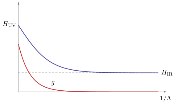
Figure 1: Schematic RG flow of $H$ and $g$.

More abstractly, consider the RG flow of the SUSY theory perturbed by two couplings breaking to partial SUSY, exactly marginal $\omega^{2}$ and irrelevant $\widetilde{\mathcal{O}}$:

$$\mathcal{S}(H)+\int g_{0}\omega^{2}+\frac{g}{\Lambda^{\gamma}}\widetilde{\mathcal{O}}.$$ (3.23)

This time $\widetilde{\mathcal{O}}$ does not have to have the above quadratic form and the discussion can be generalized easily to several $\widetilde{\mathcal{O}}$’s. On general grounds, the beta functions have the form

$$\beta_{g_{0}} = O(g),$$

$$\beta_{g} = (\gamma+O(\lambda,g_{0})+O(g))g.$$ (3.24)

The small initial coupling $g$ will flow to zero in the IR if $\gamma+O(\lambda,g_{0})$ is positive. This quantity (up to $d+$) can be interpreted as the scaling dimension of $\widetilde{\mathcal{O}}$ at the SUSY fixed point corrected by $g_{0}\omega^{2}$ and since $\omega^{2}$ is exactly marginal, it should not depend on $g_{0}$ at all: $\gamma+O(\lambda,g_{0})\rightarrow\gamma+O(\lambda)$. Operators $\widetilde{\mathcal{O}}$ breaking full SUSY to partial SUSY will reappear in section 8.3 as the susy-writable leader operators, using the terminology to be introduced below. We will see in sections 9.1 and 10 that all such operators remain irrelevant also in presence of $O(\lambda)$ corrections. Thus the coupling $g$ flows to zero, and in the IR we recover the SUSY fixed point perturbed by an exactly marginal deformation $\omega^{2}$, which as discussed in the previous section amounts to a change in $H$.

RG flow in the full Cardy theory: general plan

Let us recap. In section 2 we used the Cardy transform to rewrite the replica action in terms of the variables $\varphi,\chi_{i},\omega$. This made manifest the presence of a marginally relevant interaction close to the upper critical dimension. We then dropped some terms in the action either because they were irrelevant near $d=6$ ($\mathcal{L}_{1}$), or because they vanished in the limit $n\to 0$ ($\mathcal{L}_{2}$). This was dubbed “basic RG scenario” in section 2.4. The remaining Lagrangian $\mathcal{L}_{0}$ could be seen formally equivalent to a supersymmetric one $\mathcal{L}_{\operatorname{SUSY}}$, replacing $\text{O}(-2)$-invariant bilinears made of fields $\chi_{i}$ by $\operatorname{Sp}(2)$-invariant bilinears made out of two Grassmann fields $\psi,\bar{\psi}$. Then, in section 3.1 we discussed RG flow in the SUSY theory, concluding that it has a nontrivial RG fixed point down to $d=4$ but not in 3d. This was based on dimensional reduction and the well-known Wilson-Fisher fixed point properties. In section 3.2 we discussed the RG flow of $\mathcal{L}_{0}$ theory. Due to subtleties of the UV regulator the bare theory preserves SUSY only partially (supertranslations but not superrotations), yet at long distances full SUSY is recovered.

We will now come back to the full Cardy theory $\mathcal{L}_{0}+\mathcal{L}_{1}+\mathcal{L}_{2}$. We will discuss the RG flow in this setup and examine the validity of the basic RG scenario assumptions (a) and (b). We will work in the $\varphi,\chi_{i},\omega$ formulation rather then in the SUSY field basis $\varphi,\psi,\bar{\psi},\omega$. Indeed, the full Lagrangian contains some operators involving odd powers of $\chi_{i}$ fields (e.g. $\sum\nolimits^{\prime}\chi^{3}_{i}\varphi$) which cannot be written in terms of SUSY fermions. Such operators will play an important role in stability of the RG flow.

Our plan is as follows. In section 5 we will describe a somewhat peculiar form taken by the $S_{n}$ invariance in the Cardy basis. Here we will introduce the notion of a “leader”–the lowest-dimension part of an $S_{n}$-singlet operator transformed to the Cardy basis–and of its “followers” which are the higher-dimension parts. In the short but important section 6 we will analyze the role of $n$-suppressed terms. Here we will explain that the assumption (b) of the basic RG scenario holds, but in a subtle sense: the theory with a small but finite $n$ is gapped, but as the $n\rightarrow 0$ limit is taken, the approximately scale invariant region of the RG flow becomes longer and longer. This is different from what happens in the bond-(as opposed to field-) disordered Ising model, where the $n\neq 0$ fixed point is believed to smoothly connect to $n=0$, but it suffices for our purposes: $\mathcal{L}_{2}$ can be dropped.

With $\mathcal{L}_{2}$ out of the way, in section 7 we will focus on the $\mathcal{L}_{0}+\mathcal{L}_{1}$ RG flow, working in the strict $n=0$ limit. We will examine if some $\mathcal{L}_{1}$ perturbations (or other $S_{n}$-invariant perturbations generated by RG) which are irrelevant in $d=6-\varepsilon$ dimensions, may become relevant in lower $d$. The leader-follower distinction becomes very handy here, because as we will see the relevance of an $S_{n}$-singlet perturbation can be decided by computing the scaling dimension of the leader alone.

Next, in section 8, we will classify the leader operators, dividing them into three classes: non-susy-writable, susy-writable and susy-null. These three classes RG-mix among each other only in a triangular way, which will simplify the anomalous dimension computations (section 9). Exhaustive classification of leaders will be carried out up to dimension 12 in $d=6$, which includes one or more lowest-lying leaders in each of the three classes. Anomalous dimensions will be computed at one or two loops.

Fig. 2 is a roadmap for all these steps. Once completed, we will see in section 10 what this implies for the loss of Parisi-Sourlas SUSY.

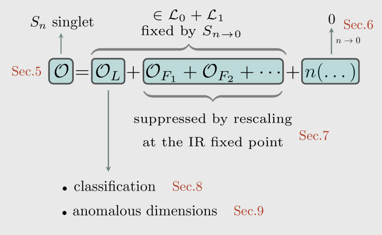
Figure 2: This figure illustrates how a generic $S_{n}$-singlet perturbation $\mathcal{O}$ is divided into various pieces (leader, followers, $n$-suppressed) and shows the sections of our paper where these pieces are discussed.

$S_{n}$ invariance in the Cardy basis

The original replicated action (2.7) is invariant under permutations of the $n$ replicas. While the Cardy transform clarifies many properties of our RG flow, it somewhat obscures this $S_{n}$ symmetry, meriting a discussion. We have permutations $\phi_{1}\leftrightarrow\phi_{i}$ and $\phi_{i}\leftrightarrow\phi_{j}$ ($i,j\in\{2,\ldots,n\}$). After Cardy transform, the latter give rise to permutations $\chi_{i}\leftrightarrow\chi_{j}$ which generate $S_{n-1}$ subgroup. This symmetry subgroup is manifest in the Cardy basis: invariance of $\mathcal{L}_{\operatorname{Cardy}}$ under it just means that $\chi_{i}$’s should enter in singlet combinations.

Consider now permutations of the former kind, $\phi_{1}\leftrightarrow\phi_{i}$. Without loss of generality we focus on $\phi_{1}\leftrightarrow\phi_{2}$ since together with $S_{n-1}$ it generates the full $S_{n}$. Applying Cardy transform with $\phi_{2}$ and $\phi_{1}$ interchanged, the relation between the new and old Cardy fields is found from the equations

$$\phi_{1} = \varphi+\frac{\omega}{2}=\varphi^{\prime}-\frac{\omega^{\prime}}{2}+\chi_{2}^{\prime},$$

$$\phi_{2} = \varphi-\frac{\omega}{2}+\chi_{2}=\varphi^{\prime}+\frac{\omega^{\prime}}{2},$$

$$\phi_{i} = \varphi-\frac{\omega}{2}+\chi_{i}=\varphi^{\prime}-\frac{\omega^{\prime}}{2}+\chi^{\prime}_{i}\qquad(i=3\ldots n),$$ (5.1)

where we renumbered the fields $\chi_{i}^{\prime}$ so that their index always runs from 2 to $n$. We thus find

$$\varphi^{\prime} = \varphi-\frac{2-n}{2(1-n)}(\omega-\chi_{2}),$$

$$\omega^{\prime} = \frac{\omega}{1-n}-\frac{n}{1-n}\chi_{2},$$

$$\chi_{2}^{\prime} = \frac{2-n}{1-n}\omega-\frac{\chi_{2}}{1-n},$$

$$\chi_{i}^{\prime} = \chi_{i}+\frac{\omega-\chi_{2}}{1-n}\qquad(i=3\ldots n).$$ (5.2)

We will mostly use the $n\rightarrow 0$ limit of this “extra” symmetry transformation, which is

$$\varphi^{\prime} = \varphi-2(\omega-\chi_{2}),$$

$$\omega^{\prime} = \omega,$$

$$\chi_{2}^{\prime} = 2\omega-\chi_{2},$$

$$\chi_{i}^{\prime} = \chi_{i}+\omega-\chi_{2}\qquad(i=3\ldots n).$$ (5.3)

Let us see how $\mathcal{L}_{\operatorname{Cardy}}$ behaves under this. The $\omega^{2}$ term in $\mathcal{L}_{0}$, Eq. (2.22), is trivially invariant. It is more interesting to check that the mass term is invariant:

$$2\varphi\omega+\sum_{i=2}^{n}\chi_{i}^{2}\rightarrow 2[\varphi-2(\omega-\chi_{2})]\omega+(2\omega-\chi_{2})^{2}+\sum_{i=3}^{n}(\chi_{i}+\omega-\chi_{2})^{2},$$ (5.4)

and using the constraint $\sum\nolimits^{\prime}\chi_{i}=0$ we see that the r.h.s. reduces to the l.h.s. Analogously the kinetic part $\partial\varphi\partial\omega+\frac{1}{2}(\partial\chi_{i})^{2}$ is also invariant.

For the quartic term, $S_{n}$ invariance is realized in a still more interesting way. The quartic term is the marginal (in $d=6$) part of the $S_{n}$ invariant term $\sigma_{4}=\sum_{i=1}^{n}\phi_{i}^{4}$ whose full $n\rightarrow 0$ limit is

$$\sigma_{4} = \left[4\omega\varphi^{3}+6\sum\nolimits^{\prime}\chi_{i}^{2}\varphi^{2}\right]_{\Delta=6}$$ (5.5)

$$+\left[4\varphi\sum\nolimits^{\prime}\chi_{i}^{3}\right]_{\Delta=7}+\left[\sum\nolimits^{\prime}\text{}\chi_{i}^{4}-6\varphi\omega\sum\nolimits^{\prime}\chi_{i}^{2}\right]_{\Delta=8}$$

$$-\left[2\omega\text{}\sum\nolimits^{\prime}\chi_{i}^{3}\right]_{\Delta=9}+\left[\frac{3}{2}\omega^{2}\text{}\sum\nolimits^{\prime}\chi_{i}^{2}+\varphi\omega^{3}\right]_{\Delta=10},$$

where we indicated the scaling dimensions in $d=6$. The irrelevant terms in the second and third lines have been assigned to the $\mathcal{L}_{1}$ part of the Lagrangian. It is now possible to check that the sum of all terms is invariant under the $n=0$ symmetry (5.3), although the first line by itself is not.

We thus learn something very important: the sum $\mathcal{L}_{0}+\mathcal{L}_{1}$ is invariant under the full $S_{n}$ symmetry in the $n\rightarrow 0$ limit (denoted $S_{n\rightarrow 0}$), while individually the two parts are invariant only under the $S_{n-1}$ subgroup permuting $\chi_{i}$’s.

And what about $\mathcal{L}_{2}$? It was originally defined as consisting of the $n$-suppressed terms, but now we can give an alternative description: $\mathcal{L}_{2}$ consists of all terms which are not invariant under the extra symmetry (5.3), nor can be made invariant by adding further terms. Consider e.g. $\varphi^{2}$, which is in $\mathcal{L}_{2}$ according to (2.24). Under the extra symmetry we have:

$$\varphi^{2}\rightarrow[\varphi-2(\omega-\chi_{2})]^{2}=\varphi^{2}-4(\omega-\chi_{2})\varphi+4(\omega-\chi_{2})^{2}.$$ (5.6)

This is obviously not invariant by itself, nor can it be made invariant by adding other terms. E.g. variation of $\varphi^{2}$ contains $-4\omega\varphi$ and a moment’s thought shows that this cannot be canceled by variation of anything.

Since the terms in $\mathcal{L}_{2}$ are not invariant under the $S_{n\rightarrow 0}$ symmetry, their coefficients must be proportional to $n$. This explains why they are “$n$-suppressed”. The advantage of this new understanding is that it is not tied to the bare Lagrangian but can be used along the RG flow. Since $\mathcal{L}_{0}+\mathcal{L}_{1}$ are $S_{n\rightarrow 0}$ invariant, they can generate $\mathcal{L}_{2}$ terms only with $n$-suppressed coefficients. This guarantees that a term $n$-suppressed in the bare Lagrangian remains $n$-suppressed at a lower RG scale.

$S_{n}$ singlets in the replicated basis

As pointed out by Brézin and De Dominicis [28], the replicated Lagrangian (2.7), in addition to the shown bare terms, will generate infinitely many extra $S_{n}$ invariant terms upon RG flow. Of course, these terms may or may not destabilize the RG flow depending on their scaling dimensions. Leaving this more complicated question for later, let us first learn to write general $S_{n}$ invariant terms (referred to as “singlets” from now on). In the replicated basis, they can be constructed as finite products:

$$\left[\sum_{i=1}^{n}A(\phi_{i})\right]\left[\sum_{j=1}^{n}B(\phi_{j})\right]\left[\sum_{k=1}^{n}C(\phi_{k})\right]\times\ldots$$ (5.7)

where $A,B,C\ldots$ are some polynomial functions of $\phi_{i}$ and of its derivatives. For most part we will be interested in scalar perturbations, which means that $A,B,C$ either do not contain derivatives, or that all derivative indices are contracted.

We will use the notation ($\sum\equiv\sum_{i=1}^{n}$)

$$\sigma_{k}=\sum\phi_{i}^{k},$$

$$\sigma_{k(\mu)}=\sum\phi_{i}^{k-1}\partial_{\mu}\phi_{i},$$

$$\sigma_{k(\mu\nu)}=\sum\phi_{i}^{k-1}\partial_{\mu}\partial_{\nu}\phi_{i},$$

$$\sigma_{k(\mu)(\nu)}=\sum\phi_{i}^{k-2}\partial_{\mu}\phi_{i}\partial_{\nu}\phi_{i},\quad\operatorname{etc}.$$ (5.8)

The fields $\sigma_{k}$ were considered in [28], and the others are natural generalizations. More singlets can be constructed by taking products of these basic building blocks.

In this notation, e.g., the bare replicated Lagrangian (quartic potential) is a linear combination of singlets

$$\sigma_{2(\mu)(\mu)},\qquad\sigma_{1}^{2},\qquad\sigma_{2},\qquad\sigma_{4}.$$ (5.9)

But we can clearly construct more singlets. E.g. with four fields and no derivatives the full list has five singlets [28]:

$$\sigma_{4},\quad\sigma_{1}\sigma_{3},\quad\sigma_{2}^{2},\quad\sigma_{1}^{2}\sigma_{2},\quad\sigma_{1}^{4}.$$ (5.10)

Still more singlets are obtained by increasing the number of fields or introducing derivatives. What are the scaling dimension of the corresponding fixed point perturbations? Can they become relevant as the dimension is lowered? We will study these questions systematically in the subsequent sections.

Feldman [30] discussed a family of singlet operators $\mathcal{F}_{k}$ $(k\in 2\mathbb{N})$ given by

$$\mathcal{F}_{k} = \sum_{i,j=1}^{n}(\phi_{i}-\phi_{j})^{k}=\sum_{l=1}^{k-1}(-1)^{l}\binom{k}{l}\sigma_{l}\sigma_{k-l}$$ (5.11)

(the $l=0,k$ terms vanish for $n\rightarrow 0$). Operators $\mathcal{F}_{4}$ and $\mathcal{F}_{6}$ will play an important role in our work.

$S_{n}$ singlets in the Cardy basis

Applying the Cardy transform to any singlet in the replicated basis, we get an $S_{n\rightarrow 0}$ singlet in the Cardy basis. We have already seen such expressions above, e.g.

$$\sigma_{2}=2\varphi\omega+\sum\nolimits^{\prime}\chi_{i}^{2},$$ (5.12)

while $\sigma_{4}$ is given in (5.5). We will use this procedure to construct all singlets in the Cardy basis. Generality of this method follows from the fact that the Cardy transform is an invertible linear transformation of the field basis. We have the following master formula (here and below we drop terms vanishing in the $n=0$ limit):

$$\sum_{i=1}^{n}A(\phi_{i}) = A\left(\varphi+\frac{\omega}{2}\right)+\sum\nolimits^{\prime}A\left(\varphi-\frac{\omega}{2}+\chi_{i}\right)$$ (5.14)

$$= \frac{\delta A}{\delta\varphi}(\varphi)\omega+\frac{1}{2}\frac{\delta^{2}A}{\delta\varphi^{2}}(\varphi)\sum\nolimits^{\prime}\chi_{i}^{2}$$

$$+\sum_{k=3}^{\infty}\frac{1}{k!}\frac{\delta^{k}A}{\delta\varphi^{k}}(\varphi)\left[\left(\frac{\omega}{2}\right)^{k}+\sum\nolimits^{\prime}\left(-\frac{\omega}{2}+\chi_{i}\right)^{k}\right].$$

Let us introduce some useful terminology. By composite operators (composites, for short) we will mean products of Cardy fields, their derivatives, and linear combinations thereof. To each product composite we assign a classical scaling dimension which is the sum of dimensions of its constituents, Eq. (2.16). A linear combination of composites has a “well-defined classical dimension” if all terms have the same dimension. Later on, we will also discuss anomalous dimensions due to interactions. Due to mixing, only some special linear combinations will have well-defined anomalous dimensions.

In this terminology, the terms in the first line of (5.14) have the same classical dimension, while those in the second line have a higher dimension. For singlets involving at most two fields ($\sigma_{1}$, $\sigma_{2}$, $\sigma_{1(\mu)}$, $\sigma_{2(\mu)}$, etc), the second line is absent ($\delta^{k}A/\delta\varphi^{k}\equiv 0$). Such fields, and products thereof, are special: they have well-defined classical dimensions in the Cardy basis. One example is (5.12) where both composites have dimension $d-2$. Any other singlet will becomes a linear combination of composites of different dimensions in the Cardy basis. We have seen one example in (5.5).

Given any singlet $\mathcal{O}$, we can split it into parts with definite classical dimension, which will come in unit steps:

$$\mathcal{O}=[\mathcal{O}]_{\Delta}+[\mathcal{O}]_{\Delta+1}+\ldots$$ (5.15)

We will call the “leader” the lowest scaling dimension part of $\mathcal{O}$, that is $[\mathcal{O}]_{\Delta}$, while $[\mathcal{O}]_{\Delta+k}$ with $k\geqslant 1$ will be called “followers”. E.g. the first line of the r.h.s. of (5.5) is the leader of $\sigma_{4}$, while the subsequent lines contains the followers. The rationale for this terminology will become clear in section 7.

As an exercise which will turn out useful later on, let us transform Feldman operators to the Cardy basis and extract the leader. Using definition (5.11) we have:

$$\mathcal{F}_{k} = 2\sum_{i=2}^{n}(\omega-\chi_{i})^{k}+\sum_{i,j=2}^{n}(\chi_{i}-\chi_{j})^{k}.$$ (5.16)

In particular there is no dependence on $\varphi$ for this very special operator. Expanding we have

$$\mathcal{F}_{k} = \sum_{l=2}^{k-2}(-1)^{l}\binom{k}{l}\left(\sum\nolimits^{\prime}\chi^{l}_{i}\right)\left(\sum\nolimits^{\prime}\chi^{k-l}_{i}\right)$$

$$-2k\omega\left(\sum\nolimits^{\prime}\chi^{k-1}_{i}\right)+\ldots$$

where we used $\sum\nolimits^{\prime}\chi_{i}=0$ and that $\sum\nolimits^{\prime}\chi_{i}^{k}$ cancels between the two terms for $n\rightarrow 0$. This shows the leader (first line) and the first follower for $k\geqslant 4$. (For $k=2$ the shown terms vanish and $\mathcal{F}_{2}=-2\omega^{2}$.)

The $n$-suppressed terms

Following our plan to clarify step-by-step the basic RG scenario of section 2.4, we will discuss here the effects associated with the $n$-suppressed terms, which were grouped in the $\mathcal{L}_{2}$ part of the Cardy-transformed Lagrangian (2.25). As explained in section 5, these terms can be alternatively characterized as those which break the $S_{n\rightarrow 0}$ symmetry of the $\mathcal{L}_{0}+\mathcal{L}_{1}$ Lagrangian. This implies that the terms $n$-suppressed in the bare Lagrangian remain $n$-suppressed along the RG flow. If we set $n=0$, these terms vanish in the bare Lagrangian and are not regenerated in the RG flow. Still, it is instructive to analyze what would happen if we worked at a tiny but nonzero $n$. Note that $\mathcal{L}_{2}$ contains several relevant terms so that, while $n$-suppressed, they grow in the IR. One such term is the operator $\varphi^{2}$, which comes from the operator $\sigma_{2}\ni n\varphi^{2}$ (while the $n=0$ part of $\sigma_{2}$ goes into $\mathcal{L}_{0}$). What would be the role of these terms for the IR behavior of the theory?

For concreteness let us just focus on this very operator $\varphi^{2}$, the discussion being similar for any other relevant part of $\mathcal{L}_{2}$ such as $\varphi^{4}$ or $(\partial\varphi)^{2}$. We thus consider $\mathcal{L}_{0}$ action perturbed by

$$g_{2}\,\Lambda_{\mathrm{UV}}^{4}\int d^{d}x\hskip 1.69998pt\varphi^{2},$$ (6.1)

with $\Lambda_{\mathrm{UV}}$ the UV cutoff energy scale, and $g_{2}$ a dimensionless coupling. The power of $\Lambda_{\mathrm{UV}}$ is fixed by the dimension of the perturbing operator, $d-4$ in the case at hand.

We are considering the situation when in absence of the perturbation the $\mathcal{L}_{0}$ part of the action flows to an IR fixed point. When we add the perturbation the coupling $g_{2}$ starts growing. Since $g_{2}$ starts at order-$n$ at the UV scale, it reaches order-1 values at the scale

$$\Lambda_{\mathrm{IR}}\sim n^{1/4}\Lambda_{\mathrm{UV}}\hskip 1.69998pt.$$ (6.2)

At that point we can no longer treat it as a small perturbation.

The conclusions from this discussion is that, first of all, the $n=0$ fixed point is unstable with respect to turning on nonzero $n$. For $n$ tiny but nonzero, the RG trajectory stays for a long time near the fixed point before finally deviating. Thus, for a very small $n$, we expect that in a range of distances the theory will be approximately described by the $n=0$ fixed point and will have an approximate scale invariance, and this range will become longer and longer as $n\to 0$. However, no matter how small $n$ is, the trajectory eventually deviates (see Fig. 3).

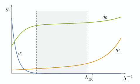
Figure 3: Schematic RG flow (from short to long distances) including $n$-suppressed terms. The flow has three parts (left to right): (1) the transitory part where the couplings $g_{0}$ of $\mathcal{L}_{0}$ flows to a fixed point, while the irrelevant couplings $g_{1}$ of $\mathcal{L}_{1}$ go to zero; (2) the shaded part where the flow stays close to the $\mathcal{L}_{0}$ fixed point; (3) the part where the relevant $\mathcal{L}_{2}$ terms finally grow to overcome suppression by $n$, and the flow deviates from the fixed point.

We do not know what happens with the small $n$ trajectory afterwards – it may flow to a gapped phase or to another fixed point. Note that even if the trajectory flows to a fixed point, such a fixed point would have no significance for the disordered physics, not being continuously connected to the $n=0$ fixed point. One example of such a fixed point for nonzero $n$ can be found in the work of Brézin and De Dominicis [28]. Their fixed point has couplings scaling as inverse powers of $n$, a clear feature of being disconnected from $n=0$. For the above reasons we will not consider their fixed point any further in the main text, although we provide more details in App. A.9.

To summarize, when $n\to 0$, the range in which the flow is close to the $\mathcal{L}_{0}$ fixed point becomes infinitely large. This clarifies in which sense the $n$-suppressed terms can be safely discarded in the limit $n\to 0$.

RG flow in the $\mathcal{L}_{0}+\mathcal{L}_{1}$ theory

At this point we are left with studying the RG flow in the theory consisting of $\mathcal{L}_{0}+\mathcal{L}_{1}$ part of the Cardy Lagrangian, working in the strict $n=0$ limit. As discussed in section 3, the $\mathcal{L}_{0}$ theory by itself flows to an IR fixed point equivalent to the SUSY fixed point of $\mathcal{L}_{\operatorname{SUSY}}$. The key remaining question is whether this RG flow is stable under $\mathcal{L}_{1}$ perturbations.

In the original definition, $\mathcal{L}_{1}$ included all terms irrelevant in $d$ just below 6, coming from the replicated bare Lagrangian with the quartic potential. This was not completely general: the bare Lagrangian can be expected to contain any possible $\mathbb{Z}_{2}$-even $S_{n}$ singlets, and even if not initially, included such terms will be generated under RG flow [28]. From now on we will extend the definition of the bare Lagrangian to include all $\mathbb{Z}_{2}$-even $S_{n}$ singlets. E.g., at the quartic level we should consider all terms given in (5.10) (while only the first of these five singlets was included so far). It is easy to see that with the new definition we do not get any additional relevant terms in $d=6-\varepsilon$. So all new terms end up in $\mathcal{L}_{1}$.

Now that we have the full bare Lagrangian, we should ask: can it be that some perturbations, while irrelevant near 6d, become relevant for smaller $d$? If this happens, the $\mathcal{L}_{0}$ fixed point will not be reached for those $d$. The RG flow will be instead deviated to another fixed point, which does not have SUSY if the new relevant interaction is SUSY-breaking (something to be checked).

We wish to explore this mechanism for the loss of Parisi-Sourlas SUSY. The problem is well defined, at least in perturbation theory: we need to consider $\mathcal{L}_{1}$ perturbations one by one, and see which of them get anomalous dimensions of sign and size likely to render them relevant. We are interested in stability with respect to $S_{n}$ singlet perturbations, because only such perturbations are present in the microscopic replicated Lagrangian (i.e. before the Cardy transform).

Leader and followers: quartic term

In section 5 we saw that after the Cardy transform, a generic $S_{n}$ singlet is a sum of the leader (the lowest scaling-dimension part) and the followers (higher scaling dimension parts). The quadratic terms in the replicated Lagrangian do not have any followers, while the quartic term has both the leader and the followers, see (5.5).

It is instructive to consider first the RG flow of the $\mathcal{L}_{0}+\mathcal{L}_{1}$ theory truncated just to the quartic perturbation (5.5). We start the RG flow at an energy scale $\Lambda$ with the Lagrangian in the Cardy basis (in equations below we use the notation $\chi_{i}^{k}\equiv\sum_{i}^{\prime}\chi_{i}^{k}$)

$$\partial\varphi\partial\omega+\frac{1}{2}(\partial\chi_{i})^{2}-\frac{H}{2}\omega^{2}+\frac{m^{2}}{2}\left(2\varphi\omega+\chi_{i}^{2}\right)+\frac{\lambda}{4!}\left[\left(4\omega\varphi^{3}+6\chi_{i}^{2}\varphi^{2}\right)+4\varphi\chi_{i}^{3}+\ldots\right],$$ (7.1)

where $\ldots$ stands for the other $\sigma_{4}$ followers visible in (5.5). Performing the integrating-out step down to the energy scale $\Lambda^{\prime}=\Lambda/b$ (but not yet any field rescaling), we will find an effective Lagrangian

$$Z_{1}\left[\partial\varphi\partial\omega+\frac{1}{2}(\partial\chi_{i})^{2}\right]-Z_{2}\frac{H}{2}\omega^{2}+(m^{\prime})^{2}\left(\varphi\omega+\frac{1}{2}\chi_{i}^{2}\right)+\frac{\lambda^{\prime}}{4!}\left[\left(4\omega\varphi^{3}+6\chi_{i}^{2}\varphi^{2}\right)+4\varphi\chi_{i}^{3}+\ldots\right].$$ (7.2)

Crucially, $S_{n}$ invariance guarantees that the kinetic terms $\partial\varphi\partial\omega+\frac{1}{2}(\partial\chi_{i})^{2}$, the mass terms $2\varphi\omega+\chi_{i}^{2}$, and the whole quartic interaction renormalize by overall rescaling, since the form of these terms is fixed uniquely by transforming $\sigma_{2(\mu)(\mu)}$, $\sigma_{2}$ and $\sigma_{4}$ to the Cardy basis. We now perform field rescaling

$$\varphi(x) \rightarrow Z_{1}^{-1/2}b^{-\Delta_{\varphi}^{0}}\varphi(x/b),$$

$$\chi_{i}(x) \rightarrow Z_{1}^{-1/2}b^{-\Delta_{\chi}^{0}}\chi_{i}(x/b),$$ (7.3)

$$\omega(x) \rightarrow Z_{1}^{-1/2}b^{-\Delta_{\omega}^{0}}\omega(x/b),$$

where $\Delta_{\varphi}^{0},\Delta_{\chi_{i}}^{0},\Delta_{\omega}^{0}$ are the Gaussian fixed point dimensions (2.16). After rescaling, the fields again have momenta up to $\Lambda$ while the Lagrangian becomes:

$$\partial\varphi\partial\omega+\frac{1}{2}(\partial\chi_{i})^{2}-\frac{Z_{2}}{Z_{1}}\frac{H}{2}\omega^{2}+\frac{(m^{\prime})^{2}b^{2}}{Z_{1}}\left(\varphi\omega+\frac{1}{2}\chi_{i}^{2}\right)$$

$$+\frac{\lambda^{\prime}b^{\varepsilon}}{4!Z_{1}^{2}}\left[\left(4\omega\varphi^{3}+6\chi_{i}^{2}\varphi^{2}\right)+\frac{1}{b}4\varphi\chi_{i}^{3}+\frac{1}{b^{2}}\left(\text{}\chi_{i}^{4}-6\varphi\omega\chi_{i}^{2}\right)-\frac{1}{b^{3}}2\omega\text{}\chi_{i}^{3}+\frac{1}{b^{4}}\left(\frac{3}{2}\omega^{2}\text{}\chi_{i}^{2}+\varphi\omega^{3}\right)\right].$$ (7.4)

We see that in general $Z_{2}\neq Z_{1}$ and $H$ will be renormalized. However as discussed in section 3.2 we can expect that this effect is transient and disappears in deep infrared so that $H$ flows to a constant. Here we are focusing on the behavior of the $\sigma_{4}$ followers, this time written in full. We see that their coefficients rescale with an additional positive integer power of $b$ compared to that of the leader. But, apart from this additional rescaling, the relative coefficients stay fixed because determined by $S_{n}$ invariance. This explain our choice for the leader-follower terminology.

After many RG steps the coefficients of the followers will flow to zero, and we approach the fixed point of the $\mathcal{L}_{0}$ theory. It is not so surprising that the follower coefficients flow to zero as these operators are irrelevant. What is more surprising is that the coefficients of these irrelevant terms go to zero in a prescribed fashion. This feature of the $\mathcal{L}_{0}+\mathcal{L}_{1}$ RG flow is dictated by $S_{n}$ invariance.

We can rephrase the above conclusions as follows. Consider the perturbation $(\delta\lambda)\sigma_{4}$ on top of the $\mathcal{L}_{0}$ fixed point, splitting it into the leader and the followers:

$$(\delta\lambda)\sigma_{4}=\delta\lambda\left[\left(4\omega\varphi^{3}+6\chi_{i}^{2}\varphi^{2}\right)+4\varphi\chi_{i}^{3}+\ldots\right].$$ (7.5)

At a lower scale $\Lambda/b$ the perturbation will become

$$\delta\lambda(b)\left[\left(4\omega\varphi^{3}+6\chi_{i}^{2}\varphi^{2}\right)+\frac{1}{b}4\varphi\chi_{i}^{3}+\ldots\right].$$ (7.6)

We see here two effects. First, the coefficients of the followers are suppressed compared to that of the leader by integer powers of $b$. Second, assuming that the fixed point is reached, $\delta\lambda(b)$ flows to zero (which is the same as $\lambda$ flowing to a constant). Let us introduce the RG eigenvalue $y$ for $\delta\lambda$:

$$\frac{d}{d\log b}\delta\lambda=-y\delta\lambda,$$ (7.7)

where $y$ must be positive for $\delta\lambda$ to flow to zero.

The simplest way to compute $y$ is to go to deep IR. There the coefficients of the followers are tiny and can be neglected. We are therefore reduced to the problem of computing the anomalous dimension of the leader as a perturbation of the $\mathcal{L}_{0}$ fixed point. This recipe is a key simplification: it would have been much more awkward to compute anomalous dimension if we had to keep track of both the leader and the followers.

For the quartic coupling case at hand, $y$ is related to the anomalous dimension of $\left(4\omega\varphi^{3}+6\chi_{i}^{2}\varphi^{2}\right)$ perturbing the $\mathcal{L}_{0}$ fixed point. This being a susy-writable operator, its anomalous dimension is the same as that of $\left(4\omega\varphi^{3}+3\psi\bar{\psi}\varphi^{2}\right)$ perturbing the $\mathcal{L}_{\operatorname{SUSY}}$ fixed point. In turn, by dimensional reduction, this is the same as the anomalous dimension of $\widehat{\phi}^{4}$ at the Wilson-Fisher fixed point in $d-2$ dimensions (see section 9.1 below). The latter operator is irrelevant since the Wilson-Fisher fixed point has only one relevant $\mathbb{Z}_{2}$ even singlet $(\widehat{\phi}^{2})$, hence indeed $y>0$.

Leader and followers: general case

We will now generalize the quartic coupling perturbation considered in the previous section to any other singlet perturbation $g\mathcal{O}$ inside the $\mathcal{L}_{0}+\mathcal{L}_{1}$ flow. Near the $\mathcal{L}_{0}$ fixed point, this perturbation takes the form

$$g(b)\left[\mathcal{O}_{L}+\frac{1}{b}\mathcal{O}_{F1}+\frac{1}{b^{2}}\mathcal{O}_{F2}+\ldots+\right],\qquad\frac{d}{d\log b}g=-y_{\mathcal{O}}g,$$ (7.8)

where $\mathcal{O}_{L}$ is the leader, while $\mathcal{O}_{F1},\mathcal{O}_{F2},\ldots$ are the followers. If the leader coefficient flows to zero ($y_{\mathcal{O}}>0$), the follower coefficients flow to zero as well, and faster. The RG eigenvalue $y_{\mathcal{O}}$ can be computed as

$$y_{\mathcal{O}}=\Delta(\mathcal{O}_{L})-d,$$ (7.9)

where $\Delta(\mathcal{O}_{L})$ is the scaling dimension of $\mathcal{O}_{L}$ as a perturbation of the $\mathcal{L}_{0}$ fixed point. A very convenient feature is that the followers do not enter into the latter computation.

We are thus converging on a well-defined problem of quantum field theory. We have to classify all perturbations of the $\mathcal{L}_{0}$ fixed point which can be realized as leaders of $\mathbb{Z}_{2}$-even $S_{n}$ singlets, and compute their anomalous dimensions. If one of these becomes relevant, stability of the $\mathcal{L}_{0}$ fixed point is lost. This program will be realized in section 8 and 9 below.

Followers as individual $\mathcal{L}_{0}$ perturbations

The reader may find somewhat puzzling the feature of the above discussion that followers completely “go for the ride”. In other words, we are not supposed to consider followers as individual perturbations of the $\mathcal{L}_{0}$ fixed point. Let us give a few more explanations concerning this fact. We are studying stability of the $\mathcal{L}_{0}$ fixed point in the IR, by adding to it infinitesimal $S_{n}$ singlet perturbations and seeing if they grow or decay. In this setup, perturbing the $\mathcal{L}_{0}$ fixed point by a follower alone would not be consistent: the follower always accompanies a leader, whose coefficient is enhanced by the RG flow with respect to that of the follower. That is why the correct procedure is to perturb infinitesimally by the leader, while the follower perturbation then is “doubly infinitesimal” in IR, and can be neglected.

But what if we nevertheless perturb the $\mathcal{L}_{0}$ fixed point by a follower alone and compute the anomalous dimension of such a perturbation? What would be the physical meaning of such a computation? The answer is instructive. In addition to $S_{n}$ singlet perturbations, the $\mathcal{L}_{0}+\mathcal{L}_{1}$ RG flow possesses perturbations breaking $S_{n}$ invariance. Were we to perturb the $\mathcal{L}_{0}$ fixed point by a follower alone, we would be computing dimensions of such $S_{n}$-breaking perturbations. These perturbations are not important for the problem of $S_{n}$-invariant RG stability studied in this paper, but they do exist.

To convince ourselves in the reality of $S_{n}$-breaking perturbations, we found useful the following toy model. Consider the $S_{n}$-invariant RG flow with initial conditions corresponding to the quadratic part of the $\mathcal{L}_{0}$ Lagrangian perturbed by 5 quartic singlets without derivatives from Eq. (5.10):

$$\left[\partial\varphi\partial\omega+\frac{1}{2}\partial\chi_{i}\partial\chi_{i}-\frac{H}{2}\omega^{2}\right]+h_{1}\sigma_{4}+h_{2}\sigma_{2}^{2}+h_{3}\sigma_{1}\sigma_{3}+h_{4}\sigma_{1}^{2}\sigma_{2}+h_{5}\sigma_{1}^{4}.$$ (7.10)

When we transform these singlets into the Cardy basis, we get a total of 11 monomials. We then  consider a more general RG flow introducing 11 independent couplings for each of these monomials:

$$\begin{array}[]{l}\left[\partial\varphi\partial\omega+\frac{1}{2}\partial\chi_{i}\partial\chi_{i}-\frac{H}{2}\omega^{2}\right]+6g_{1}\varphi^{2}\chi_{i}^{2}+4g_{2}\varphi^{3}\omega+4g_{3}\varphi\chi_{i}^{3}+g_{4}\chi_{i}^{4}\\ \hskip 40.00006pt+g_{5}\varphi\omega\chi_{i}^{2}+g_{6}\omega\chi_{i}^{3}+g_{7}\omega^{2}\chi_{i}^{2}+g_{8}\varphi\omega^{3}+g_{9}\chi_{i}^{4}+g_{10}\varphi\omega\chi_{i}^{2}+g_{11}\omega^{4}.\end{array}$$ (7.11)

When these 11 couplings are set to particular linear combinations of 5 $h_{i}$’s, we are back to the $S_{n}$-invariant flow (7.10), while when we relax this condition, we get an $S_{n}$-breaking RG flow. In this setup we can do renormalization and see how these couplings evolve when we approach the IR fixed point. These computations are carried out in Appendix B, and they give a concrete illustration and a confirmation of the picture developed above.

Classification of leaders

As the first step of the program set in section 7, let us classify the $\mathbb{Z}_{2}$-even $S_{n}$ singlet leader operators. Of course, the total number of leaders is infinite. We will carry out a detailed classification for leaders up to scaling dimension $12$ in $d=6$, and we will make some comments about operators of arbitrarily high dimensions. This will be sufficient for our goal of understanding the loss of stability of the $\mathcal{L}_{0}$ fixed point.

We will pay close attention to symmetries. Symmetries control mixing of operators under RG evolution, importantly for the next section where we compute anomalous dimensions. We know that the $\mathcal{L}_{0}$ fixed point has Parisi-Sourlas supersymmetry upon replacing $\chi$ bilinears by $\psi$ bilinears. Some leaders (the susy-writable ones) can thus be located inside SUSY multiplets. Their anomalous dimensions can then be determined easily, by reusing known Wilson-Fisher results. This method is not available for leaders which are not susy-writable, whose anomalous dimensions will be computed independently starting from the $\mathcal{L}_{0}$ Lagrangian.

General remarks

We are interested in classifying the scalar leader operators up to classical dimension $\Delta_{\max}=12$ in $d=6$. A general singlet operator is constructed, in the replicated basis, as a product

$$\mathcal{O}=A_{k_{1}}\ldots A_{k_{p}},$$ (8.1)

where each $A_{k}$ is either $\sigma_{k}$ or one of its dressings by derivatives, Eq. (5.8). The classical scaling dimension of the leader will be

$$\Delta(\mathcal{O}_{L})=N_{\phi}+2p+N_{\operatorname{der}},$$ (8.2)

where $N_{\phi}=k_{1}+\ldots+k_{p}$ is the total power of $\phi$ in $\mathcal{O}$ (an even number for the considered $\mathbb{Z}_{2}$-even fields), and $N_{\operatorname{der}}$ is the total number of derivatives (also even, since indices are contracted to get a scalar). The $N_{\phi}+2p$ in (8.2) is obtained when we replace in each $A_{k_{i}}$ one $\phi$ by $\omega$ and the rest by $\varphi$, as in the first term in Eq. (5.14). Linear combinations of operators (8.1) may have leaders of higher dimensions than (8.2) if the leading terms cancel.

So we need to consider all possible products (8.1) such that $N_{\phi}+2p+N_{\operatorname{der}}\leqslant\Delta_{\max}$, do the Cardy transform, and separate the leaders. Let us show how this works for the case $N_{\phi}=4$, $N_{\operatorname{der}}=0$. The basis of singlets is given in Eq. (5.10). Performing the Cardy transform we find:

$$\sigma_{4} = \left[4\omega\varphi^{3}+6\chi_{i}^{2}\varphi^{2}\right]_{\Delta=6}+\ldots,$$

$$\sigma_{1}\sigma_{3} = [3\varphi^{2}\omega^{2}+3\varphi\omega\chi_{i}^{2}]_{\Delta=8}+\ldots,$$

$$\sigma_{2}^{2} = [4\varphi^{2}\omega^{2}+4\varphi\omega\chi_{i}^{2}+(\chi_{i}^{2})^{2}]_{\Delta=8},$$ (8.3)

$$\sigma_{1}^{2}\sigma_{2} = [2\varphi\omega^{3}+\omega^{2}\chi_{i}^{2}]_{\Delta=10},$$

$$\sigma_{1}^{4} = [\omega^{4}]_{\Delta=12}.$$

Here are below we will continue to omit $\sum\nolimits^{\prime}$: $\chi_{i}^{k}\equiv\sum\nolimits^{\prime}\chi_{i}^{k}$, $(\chi_{i}^{2})^{2}\equiv\left(\sum\nolimits^{\prime}\chi_{i}^{2}\right)^{2}$, etc.

Recall that the operators involving $\chi_{i}$’s only in $O(n-2)$ symmetric combinations, like $\chi_{i}^{2}$, are called susy-writable. Their correlators can be computed in the SUSY theory $\mathcal{L}_{\operatorname{SUSY}}$ replacing $\chi$ bilinears by $\psi$ bilinears: $\chi_{i}^{2}\rightarrow 2\psi\bar{\psi}$, etc. The full rules are given in Appendix C.

We will use the name “susy-writable” only for $O(n-2)$ invariant operators which do not vanish upon the SUSY substitution of $\chi$’s by $\psi$’s. Operators which do vanish, because of the Grassmann nature of the $\psi$ and $\bar{\psi}$, will be called “susy-null”. The simplest example is $(\chi_{i}^{2})^{2}$, which maps to $(2\psi\bar{\psi})^{2}\equiv 0$. Although one might think that susy-null operators do not have any physical effect, this is not quite true because they may have non-null followers (see section 8.4 below). The susy-null operators will not mix with susy-writable nor with non-susy-writable operators under RG, which is another reason to put them into a separate category.

Now, in (8.3), $\sigma_{1}\sigma_{3}$ and $\sigma_{2}^{2}$ have the same susy-writable part of their leader, up to a constant factor We thus can perform a linear transformation to exhibit a singlet with a purely susy-null leader:

$$\sigma_{2}^{2}-\frac{4}{3}\sigma_{1}\sigma_{3}=\frac{1}{6}\mathcal{F}_{4}=[(\chi_{i}^{2})^{2}]_{\Delta=8}-\frac{4}{3}[\omega\chi_{i}^{3}]_{\Delta=9}+\ldots,$$ (8.4)

where we also exhibited the non-susy-writable follower, coming from $\sigma_{1}\sigma_{3}$. Interestingly, this special linear combination turns out proportional to the Feldman operator $\mathcal{F}_{4}$, see Eqs. (5.11), (5.2).

This completes classification of leaders with $N_{\phi}=4$, $N_{\operatorname{der}}=0$ (see Table 1). We stress that the leader type (susy-writable, non-susy-writable or susy-null) is determined based on the expression for the leader, not for the followers.

Singlet	Leader($+1^{\operatorname{st}}$ follower if susy-null)	Leader type
$\sigma_{4}$	$\left[4\omega\varphi^{3}+6\varphi\chi_{i}^{2}\right]_{\Delta=6}$	susy-writable
$\sigma_{1}\sigma_{3}$	$[3\varphi^{2}\omega^{2}+3\varphi\omega\chi_{i}^{2}]_{\Delta=8}$	susy-writable
$\frac{1}{6}\mathcal{F}_{4}=\sigma_{2}^{2}-\frac{4}{3}\sigma_{1}\sigma_{3}$	$[(\chi_{i}^{2})^{2}]_{\Delta=8}-\frac{4}{3}[\omega\chi_{i}^{3}]_{\Delta=9}$	susy-null
$\sigma_{1}^{2}\sigma_{2}$	$[2\varphi\omega^{3}+\omega^{2}\chi_{i}^{2}]_{\Delta=10}$	susy-writable
$\sigma_{1}^{4}$	$[\omega^{4}]_{\Delta=12}$	susy-writable

Table 1: Leaders with $N_{\phi}=4$, $N_{\operatorname{der}}=0$.

The described procedure can be analogously carried out for any $N_{\phi}$ and $N_{\operatorname{der}}$ (see Appendix D). When classifying leaders containing derivatives, we separate total derivatives since those do not affect RG stability, and also do not mix with other operators of the same classical dimensions. We will next highlight conceptual aspects of this classification, separately for each leader type.

Non-susy-writable leaders

We start with the non-susy-writable leaders. These operators break the accidental $O(n-2)$ symmetry of the $\mathcal{L}_{0}$ Lagrangian to the $S_{n-1}$ symmetry permuting the $\chi_{i}$ fields.

One might think that non-susy-writable leaders should be more numerous than susy-writable ones because of their smaller symmetry. However this turns out not to be true. The point is that while there are many non-susy-writable operators, most of them end up being followers rather than leaders. We have seen this already in Eq. (5.5), where $\varphi\chi_{i}^{3}$, $\chi_{i}^{4}$ and $\omega\chi_{i}^{3}$ are all followers. Systematic enumeration (Appendix D) finds only one non-susy-writable leader up to $\Delta=12$, which comes from the Feldman operator $\mathcal{F}_{6}$:

$$\left(-\frac{1}{20}\mathcal{F}_{6}\right)_{L}=[(\chi_{i}^{3})^{2}-\frac{3}{2}(\chi_{i}^{2})(\chi_{i}^{4})]_{\Delta=12}.$$ (8.5)

At higher $\Delta$, non-susy-writable leaders could be constructed e.g. from the singlets

$$\sum_{i,j=1}^{n}(\phi_{i}-\phi_{j})^{6}P(\phi_{i},\phi_{j}),$$ (8.6)

with $P(\phi_{i},\phi_{j})$ an arbitrary polynomial. In particular, for $P(\phi_{i},\phi_{j})=(\phi_{i}-\phi_{j})^{k-6}$ these would be the higher Feldman operators $\mathcal{F}_{k}$ whose non-susy-writable leaders are given in Eq. (5.2). Still more non-susy-writable leaders can be obtained by dressing singlets (8.6) with derivatives, or multiplying them by other singlets. We will not attempt here a full classification.

Susy-writable leaders

Looking at Table 1 and Appendix D, we see that most leaders up to $\Delta\leqslant 12$ are susy-writable. It would be somewhat tedious to have to compute the anomalous dimensions of all these operators. Fortunately this turns out unnecessary because general arguments (section 9.1) will establish that most of them are guaranteed to be irrelevant. But before we come to that, let us have a general discussion of this class of operators.

We will refer to susy-writable leaders transformed to SUSY fields as “susy-written”. Consider first the following question: what distinguishes susy-written leaders from all other operators of the SUSY theory? As one may expect, this has a neat answer based on symmetry, which is as follows: The susy-written leaders correspond to supertranslation-invariant Sp(2)-invariant operators. In other words, supertranslations (3.2) and $\operatorname{Sp}(2)$ take the role of $S_{n}$ in fixing linear combinations corresponding to leaders.

Let’s explain how this comes about. The Sp(2) invariance acting on $\psi,\bar{\psi}$ is manifest in the rule (C.4). As an example of supertranslation invariance, consider susy-writable leaders in Table 1. Transforming to SUSY fields we get $\varphi^{3}\omega+3\varphi^{2}\psi\bar{\psi}$, $\varphi^{2}\omega^{2}+2\varphi\omega\psi\bar{\psi}$, $\varphi\omega^{3}+\omega^{2}\psi\bar{\psi}$, $\omega^{4}$. Indeed these are all invariant under $\delta\varphi=-\varepsilon\bar{\psi},\delta\psi=\varepsilon\omega,\delta\bar{\psi}=\delta\omega=0$, and only for these relative coefficients. More generally, susy-writable leaders appear from terms in the first line of Eq. (5.14), and it is easy to check that these become supertranslation-invariant upon passing to SUSY fields. This statement remains true also in presence of derivatives. It would be interesting to give a formal general proof, although we have tested this property so extensively that we are absolutely sure in its validity.

As any $\mathcal{L}_{\operatorname{SUSY}}$ operator, any susy-written leader can be expressed in terms of superfield $\Phi$ given in (2.28) and its (super)derivatives. E.g.

$$\varphi^{3}\omega+3\varphi^{2}\psi\bar{\psi}=\Phi^{3}\Phi_{,\theta\bar{\theta}}+3\Phi^{2}\Phi_{,\bar{\theta}}\Phi_{,\theta}|_{\theta=\bar{\theta}=0}.$$ (8.7)

Let us think in terms of superprimaries, i.e. composite operators $\mathcal{O}$ built out of the superfield $\Phi$ which transform simply under the (super)conformal symmetry of the SUSY fixed point [1]. Superprimaries have well-defined anomalous dimensions at the SUSY fixed point, equal to those of primaries in the Wilson-Fisher fixed point in $\widehat{d}=d-2$ dimensions [1]. Identifying susy-written leaders with components of superprimaries, we will easily determine their anomalous dimensions. A general superprimary is expanded in components as ([1], Eq. (3.20))

$$\mathcal{O}^{(a)}(x,\theta,\bar{\theta})=\mathcal{O}^{(a)}_{0}(x)+\theta\mathcal{O}^{(a)}_{\theta}(x)+\bar{\theta}\mathcal{O}^{(a)}_{\bar{\theta}}(x)+\theta\bar{\theta}\boldsymbol{}\mathcal{O}^{(a)}_{\theta\bar{\theta}}(x),$$ (8.8)

where $(a)$ is a collection of $\operatorname{OSp}(d|2)$ indices if superprimary transforms in a nontrivial representation. Leaders $\Upsilon$ will be found in the component $\mathcal{O}^{(a)}_{\theta\bar{\theta}}\equiv D_{\bar{\theta}}D_{\theta}\mathcal{O}^{(a)}$ which is supertranslation invariant and has scaling dimension $\Delta_{\mathcal{O}}+2$. The indices $(a)$, if present, have to be contracted to get a scalar leader. So we will have $\Upsilon=t_{(a)}\mathcal{O}^{(a)}_{\theta\bar{\theta}}$ where $t_{(a)}$ is an $\operatorname{SO}(d)\times\operatorname{Sp}(2)$ invariant tensor, or simply $\Upsilon=\mathcal{O}_{\theta\bar{\theta}}$ if $\mathcal{O}$ is a scalar superprimary. Total derivative leaders would correspond to $x$-derivatives of superprimary components; they do not affect RG flow.

In general, $\mathcal{O}^{(a)}$ will transform under $\operatorname{OSp}(d|2)$ as a traceless tensor with mixed graded symmetry represented by a Young tableau [1]. Because of the tracelessness condition, the $\operatorname{SO}(d)\times\operatorname{Sp}(2)$ invariant tensor $t_{(a)}$ above can be chosen as a product of $\varepsilon_{pq}$’s where $p,q\in\theta,\bar{\theta}$ run over the Grassmann directions. In other words, all indices $(a)$ will be pairwise assigned to $\theta\bar{\theta}$. Since graded symmetry means antisymmetry for Grassmann directions, we may conclude that the only Young tableaux giving rise to nonzero $\operatorname{Sp}(2)$ invariant components are those of shape $(2,2,\ldots,2)$ (i.e. 2 boxes in each row). This observation is very important, as it radically reduces the number of representations we need to examine. The representations with more than 2 rows do not occur below dimension 12, and we will not discuss them except for a few comments below.

In summary, all needed susy-written scalar leaders are the highest components $\mathcal{O}^{(a)}_{\theta\bar{\theta}}$ of superprimaries in the scalar $\mathcal{S}$, spin-two $\mathcal{J}^{ab}$, or box $\mathcal{B}^{ab,cd}$ representations of $\operatorname{OSp}(d|2)$, where the graded symmetric pairs of indices $(ab)$ and $(cd)$ have to be set to $\theta\bar{\theta}$, namely:

$$\mathcal{S}_{\theta\bar{\theta}\boldsymbol{}},\qquad\mathcal{J}^{\theta\bar{\theta}}_{\theta\bar{\theta}\boldsymbol{}},\qquad\mathcal{B}^{\theta\bar{\theta},\theta\bar{\theta}}_{\theta\bar{\theta}\boldsymbol{}}.$$ (8.9)

Let us now discuss superrotations (3.3). For a leader $\Upsilon=\mathcal{O}_{\theta\bar{\theta}}$ where $\mathcal{O}$ is a scalar superprimary, superrotation transformation generalizes that of $\omega$ in (3.4):

$$\delta\Upsilon=-\varepsilon_{\mu\theta}\partial^{\mu}\mathcal{O}_{\bar{\theta}}-\varepsilon_{\mu\bar{\theta}}\partial^{\mu}\mathcal{O}_{\theta}.$$ (8.10)

This only produces total derivatives, and so $\int d^{d}x\,\Upsilon$ will be preserving superrotations (and thus full SUSY). On the other hand, leaders $\Upsilon$ built out of $\operatorname{SO}(d)\times\operatorname{Sp}(2)$-invariant components $\mathcal{O}^{(a)}_{\theta\bar{\theta}}$ of a tensor superprimary (like $\mathcal{J}^{ab}$ or $\mathcal{B}^{ab,cd}$) will superrotate to other components (in addition to the total derivative terms). For such leaders, $\int d^{d}x\,\Upsilon$ will break superrotations (and thus not preserve full SUSY).

Coming back to the problem of identifying susy-written leaders with superprimary components, we can go through the list of superprimaries, and see what the corresponding leaders are. We are to classify superprimaries of the Gaussian part of $\mathcal{L}_{\operatorname{SUSY}}$, making use of the SUSY equation of motion $D^{2}\Phi=0$.

In the sector with two superfields, the lowest two superprimaries are $\Phi^{2}$ and the super stress tensor $\mathcal{T}^{ab},$see Eq. (C.4) of [1]. Superconservation fixes the dimension of $\mathcal{T}^{ab}$ at $d-2$ for any $d$, while anomalous dimensions of $\Phi^{2}$ will be the same as for the Wilson-Fisher operator $\widehat{\phi}^{2}$. The supertranslation invariant components are $(H=2)$,

$$(\Phi^{2})_{\theta\bar{\theta}} = 2\varphi\omega+2\psi\bar{\psi},$$

$$\mathcal{T}^{\mu\mu}_{\theta\bar{\theta}} = 2\mathcal{T}^{\theta\bar{\theta}}_{\theta\bar{\theta}}=-\partial\varphi\partial\omega-\partial\psi\partial\bar{\psi}+4\omega^{2}.$$ (8.11)

The first one is the SUSY mass term, while the second is a particular linear combinations of $\partial\varphi\partial\omega+\partial\psi\partial\bar{\psi}$ and $\omega^{2}$. Another linear combination with a well-defined anomalous dimension sits in the total derivative

$$\partial^{2}(\Phi^{2})_{\theta\bar{\theta}}=4(\partial\varphi\partial\omega+\partial\psi\partial\bar{\psi}-\omega^{2}),$$ (8.12)

where one uses the Gaussian EOM $\partial^{2}\varphi=-2\omega$, $\partial^{2}(\omega,\psi,\bar{\psi})=0$.

Higher spin $l\geqslant 4$ superprimaries built out of two superfields, e.g. the spin-4 $\mathcal{J}^{abcd}$, are graded symmetric-traceless tensors. They have Young tableaux with $l$ boxes in one row.  As discussed above, such Young tableau do not give rise to supertranslation- and $\operatorname{Sp}(2)$-invariant scalars, as the corresponding components vanish by graded-symmetric tracelessness (too many $\theta$’s, e.g. $\mathcal{J}^{\theta\bar{\theta}\theta\bar{\theta}}=0$).

Let us carry out a similar exercise in the sector with four superfields. Two low-dimension superprimaries are $\Phi^{4}$ and $\Phi^{2}\mathcal{T}^{ab}$ of 6d scaling dimension 4 and 6 respectively. They give rise to supertranslation invariant components of dimension 6 and 8:

$$(\Phi^{4})_{\theta\bar{\theta}} = 4\varphi^{3}\omega+12\varphi^{2}\psi\bar{\psi},$$

$$(\Phi^{2}\mathcal{T}^{\mu\mu})_{\theta\bar{\theta}} = 6\varphi^{2}\omega^{2}+12\varphi\omega\psi\bar{\psi}$$

$$-\varphi^{2}\partial\psi\partial\bar{\psi}-2\varphi\partial\varphi(\partial\psi\bar{\psi}+\psi\partial\bar{\psi})-(\partial\varphi)^{2}\psi\bar{\psi}-\varphi\omega(\partial\varphi)^{2}-\varphi^{2}\partial\varphi\partial\omega.$$

The first one is the SUSY quartic interaction. The second one is recognized as a linear combination of the dimension 8 leaders $(\sigma_{1}\sigma_{3})_{L}=3\varphi^{2}\omega^{2}+3\varphi\omega\chi_{i}^{2}$ and $(\sigma_{4(\mu)(\mu)})_{L}=(\partial\chi_{i})^{2}\varphi^{2}+\ldots$ (see Tables 1, 6). Another linear combination corresponds to $\partial^{2}(\Phi^{4})_{\theta\bar{\theta}}$.

To extend this story to higher $\Delta$, it is useful to take into account that Parisi-Sourlas superprimaries in $6$ dimensions are in correspondence with the free massless scalar primaries in $4$ dimensions. The latter can be counted using conformal characters [33]. This gives the number of primaries and their spin for each dimension. Denoting 4d primaries as $\Delta_{j_{1},j_{2}}$ where $\Delta$ is the scaling dimension and $j_{1},j_{2}\in\mathbb{Z}/2$ label the $SO(4)$ representation, up to $\Delta=10$ we find the following counting:

$$4\operatorname{fields}: 4_{0,0},6_{1,1},7_{3/2,3/2},$$

$$2\times 8_{2,2},8_{2,0\oplus 0,2},8_{1,1},8_{0,0},$$

$$9_{5/2,5/2},9_{5/2,3/2\oplus 3/2,5/2},9_{5/2,1/2\oplus 1/2,5/2},9_{3/2,1/2\oplus 1/2,3/2},$$

$$3\times 10_{3,3},10_{3,2\oplus 2,3},2\times\overline{}10_{3,1\oplus 1,3},\overline{}2\times 10_{2,2},10_{2,1\oplus 1,2},2\times 10_{1,1},10_{0,0},$$

$$6\operatorname{fields}: 6_{0,0},8_{1,1},9_{3/2,3/2},2\times 10_{2,2},10_{2,0\oplus 0,2},10_{1,1},10_{0,0},$$

$$8\operatorname{fields}: 8_{0,0},10_{1,1}.$$

The only representations from this list giving rise to $\operatorname{SO}(d)\times\operatorname{Sp}(2)$ invariant components in 6d (which are not total derivatives) are scalars ($j_{1},j_{2}=0$), rank-2 tensors ($j_{1},j_{2}=1,1$) and mixed-symmetry 4-index tensor corresponding to the $(2,2)$ “box” Young tableau ($j_{1},j_{2}=2,0\oplus 0,2$). Mixed symmetry tensors of shape $(2,2,\ldots)$ with more than two rows are not realized in 4d, although they may exist in 6d. 6d tensors with such symmetry are examples of representations which project to zero under dimensional reduction [1] in physical dimension. However when we go to $d=4-\varepsilon$ dimensions, such representations reappear as “evanescent operators” [36, 37]. It is possible to study evanescent operators in the $\varepsilon$-expansion [37], but since their classical dimension is rather high (the lowest scalar evanescent has dimension 15 in 4d), we will not consider them in this work as already mentioned above. We will however consider the “box” tensors in full seriousness.

Susy-null leaders

Susy-null operators are closely related to susy-writable operators. Like susy-writable operators, susy-null operators are $O(n-2)$ invariant and can be mapped to the $\psi$-formulation using the map described in appendix C. The special feature of these operators compared to susy-writables is that in the $\psi$-formulation they exactly vanish. The simplest instance of this class of operator is $(\chi^{2}_{i})^{2}$ mapped to $(\psi\bar{\psi})^{2}$ which clearly vanishes because of anticommutation of $\psi$.

These operators are evidently null in the susy theory, namely any correlation function of a susy-null operator $\mathcal{O}_{\text{null}}$ with any other operator $\mathcal{O}_{\operatorname{SUSY}}^{i}$ will vanish:

$$\left\langle\mathcal{O}_{\text{null}}\mathcal{O}_{\operatorname{SUSY}}^{1}\ldots\mathcal{O}_{\operatorname{SUSY}}^{k}\right\rangle=0.$$ (8.15)

The property above of course holds also when $\mathcal{O}_{\operatorname{SUSY}}^{i}$ is itself a susy-null operator, in particular the 2-point function $\mathcal{O}_{\text{null}}$ must vanish,

$$\left\langle\mathcal{O}_{\text{null}}\mathcal{O}_{\text{null}}\right\rangle=0.$$ (8.16)

One may be tempted to discard these operators, however this conclusion is too quick. Indeed in the $\mathcal{L}_{0}$ theory we can also consider non-susy-writable operators for which the vanishing condition does not hold,

$$\left\langle\mathcal{O}_{\text{null}}\mathcal{O}^{1}_{\text{non-susy}}\ldots\mathcal{O}^{k}_{\text{non-susy}}\right\rangle\neq 0.$$ (8.17)

A simple instance of this is the 5-point function $\langle(\chi^{2}_{i})^{2}\chi_{i_{1}}\chi_{i_{2}}\chi_{i_{3}}\chi_{i_{4}}\rangle\neq 0$, as one can easily verify in free theory by Wick contractions. In this sense susy-null operators are physical operators of the $\mathcal{L}_{0}$ theory.

Because of its special structure, this class of operators satisfies very strict selection rules for mixing under RG. Namely, susy-null operators can only mix with other susy-null operators. Indeed, as the susy-writable operators, they cannot mix with non-susy-writables since the latter are invariant under a smaller symmetry group: $S_{n-1}$ symmetry instead of the accidental $O(n-2)$. Also they cannot acquire admixtures of susy-writable operators (which are not null). This must be the case, otherwise we would find that a null operator in the SUSY theory (which should be set to zero) would mix non-trivially with a non-vanishing operator. Notice however that the mixing can occur in the opposite direction: non-susy writable and susy-writable operators can acquire admixtures of susy-nulls. Schematically, we have the following triangular mixing:

susy-null $$\leftrightarrow$$ susy-null

susy-writable $$\rightarrow \mathrm{}\text{susy-writable},\quad\text{susy-null}$$ (8.18)

non-susy-writable $$\rightarrow \text{non-susy-writable},\quad\text{susy-writable},\quad\text{susy-null}.$$

More formally this block-triangular structure holds for the matrix $Z$ relating the bare and renormalized operators, see Eq. (F.11). This in particular implies that renormalized susy-writable and non-susy-writable operators with a well-defined anomalous dimension may contain a susy-null piece. On the other hand, all renormalized susy-null operators will always stay susy-null.

Now that the definition of susy-null operators is set, let us comment on which are the possible susy-null leaders with dimensions up to $12$ in $d=6$. Systematic enumeration in Appendix D produced a few instances of susy-null leaders. The first one is the unique susy-null operator at dimensions 8: this is the Feldman $\mathcal{F}_{4}$ leader which can be written as $(\chi_{i}^{2})^{2}$. Another susy-null leader is found at dimension 10: $\varphi^{2}(\chi_{i}^{2})^{2}$. At dimension $12$ there are three susy-null leaders built out of 6 fields, which can mix among themselves $\varphi\omega(\chi_{i}^{2})^{2}$, $(\chi_{i}^{2})^{3}$, $\partial_{\mu}\varphi\partial^{\mu}\varphi(\chi_{i}^{2})^{2}$. Finally, also at dimension 12, there is a unique susy-null leader built of 8 fields $\varphi^{4}(\chi_{i}^{2})^{2}$. In the next section we will go though this list and compute all their anomalous dimensions.

Fixed point destabilization

An $S_{n}$-singlet perturbation can destabilize the IR fixed point, when its leader becomes relevant. This criterion is obvious for the susy-writable and non-susy-writable leaders. The same criterion applies also for the susy-null leaders. Note that the susy-null operators by themselves do not affect the correlation functions of all operators in the susy-writable sector. However when the coefficient of a susy-null leader grows and becomes $O(1)$ (as it may happen when such a leader is relevant), it will enter and modify RG evolution equations of other perturbations. E.g., non-susy-writable leaders which were irrelevant, may become relevant in presence of such large susy-null perturbations.

There is a small loophole, because in principle it may happen that the offending susy-null coupling flows to a nearby fixed point and never becomes $O(1)$. Whether this happens of not, depends on the higher-order terms in the beta-function, and on the sign of the initial value of the RG evolving susy-null coupling. If such a fixed point does occur, SUSY observables will be unaffected. This possibility looks somewhat exotic. In this paper we will be conservative, and will count relevant susy-null leaders as potentially destabilizing perturbations.

Anomalous dimensions

In the previous section we classified the leaders of $\mathbb{Z}_{2}$-even $S_{n}$ singlets up to 6d scaling dimension 12. We will now discuss their anomalous dimensions. Some anomalous dimensions will be computed at two loops, and some at one loop. We will consider separately the three classes of leaders (susy-null, susy-writable, and non-susy-writable). We will identify in each class at least one perturbation which becomes less irrelevant as $d$ is lowered. The next section will discuss the critical dimension $d_{c}$ where these candidate perturbations may cross the relevance threshold.

We will start in section 9.1 with the susy-writable leaders, the most numerous class. Their anomalous dimensions can be determined, as discussed above, by writing them as components of supermultiplets whose dimensions are known from dimensional reduction to Wilson-Fisher theory. This strategy is not available for the susy-null and non-susy-writable leaders, whose anomalous dimensions have to be computed from scratch (sections 9.2, 9.3).

As we explained in sections 7, the anomalous dimension computation is greatly simplified by the fact that close to the IR fixed point all follower operators can be dropped. We are therefore led to consider the anomalous dimensions of leader operators in the theory defined by the Gaussian $\mathcal{L}_{0}$ Lagrangian perturbed by the interaction $4\omega\varphi^{3}+6\chi_{i}^{2}\varphi^{2}$, at its IR fixed point in $d=6-\varepsilon$ dimensions. We use dimensional regularization.

Consistency of our method to compute anomalous dimensions by restricting to the leader operators requires that leaders and followers do not mix. For susy-writable leaders this is guaranteed explicitly by their supertranslation invariance when transformed to the SUSY fields (section 8.3). From the point of view of the $\mathcal{L}_{0}$ Lagrangian the absence of leader-follower mixing may appear puzzling, since these operators may have the same classical dimensions and the same number of fields. However, our extensive checks confirm the absence of this mixing in all cases we looked at. It would be interesting to find a formal proof, based on selection rules following from $S_{n}$ invariance, and for all three classes of leaders (see section 11.1.1).

Susy-writable leaders

The general remarks in section 8.3 give many handles on the susy-writable leaders. We will now discuss their IR scaling dimension. We have one low-dimension susy-writable leader: the SUSY mass term $(\Phi^{2})_{\theta\bar{\theta}}=2\varphi\omega+2\psi\bar{\psi}$. This operator is relevant in any $d$, its anomalous dimension being the same as for the Wilson-Fisher operator $\widehat{\phi}^{2}$ in $\widehat{d}=d-2$ dimensions. The coefficient of this operator is finetuned to reach the SUSY fixed point.

Are there any other susy-writable $\mathbb{Z}_{2}$-even leaders which are relevant? As we explained, apart from total $x$-derivatives, susy-writable leaders $\Upsilon$, when transformed to the SUSY fields, are $\operatorname{SO}(d)\times\operatorname{Sp}(2)$ invariant components $\mathcal{O}^{(a)}_{\theta\bar{\theta}\boldsymbol{}}$ of superprimaries $\mathcal{O}^{(a)}$. Their scaling dimension are thus

$$\Delta_{\Upsilon}=\Delta_{\mathcal{O}}+2=\Delta_{\widehat{O}}+2,$$ (9.1)

where we used that the scaling dimension of $\mathcal{O}$ equals that of the Wilson-Fisher primary $\widehat{O}$ to which $\mathcal{O}$ projects under dimensional reduction [1] (see also appendix H.1 for a few one-loop examples). We have seen above the example $\widehat{O}=\widehat{\phi}^{2}$ for $\mathcal{O}=\Phi^{2}$. By Eq. (9.1), $\Upsilon$ is relevant $d$ dimensions if and only if $\widehat{O}$ is relevant in $\widehat{d}$ dimensions:

$$\Delta_{\Upsilon}<d\quad\Longleftrightarrow\quad\Delta_{\widehat{O}}<\widehat{d}=d-2.$$ (9.2)

In addition, as mentioned in section 8.3, we are interested in operators $\widehat{O}$ which are either scalars, spin-2 tensors, or $2\times 2$ “box” Young tableau mixed symmetry tensors, since otherwise $\mathcal{O}$ will not have $\operatorname{SO}(d)\times\operatorname{Sp}(2)$ invariant components. Let us then discuss what is known about the spectrum of such $\mathbb{Z}_{2}$-even operators at the Wilson-Fisher (WF) fixed point.

For any $\widehat{d}$ the WF fixed point has one $\mathbb{Z}_{2}$-even relevant scalar, $\widehat{\phi}^{2}$, connected to the relevant SUSY mass term by the above argument. All other $\mathbb{Z}_{2}$-even scalars are irrelevant, which corresponds to the fact that the Ising phase transition is reached by tuning one $\mathbb{Z}_{2}$ even parameter (temperature).

In the spin-2 sector the lowest operator is the stress tensor, of dimension exactly $\widehat{d}$. All other spin-2 operators are irrelevant in 4d and expected to stay irrelevant in $\widehat{d}<4$, by two arguments. First, we have the unitarity bound $\Delta\geqslant\widehat{d}$ for any spin-2 primary in a unitary CFT. This argument is rigorous for integer $\widehat{d}$ but it has a caveat for intermediate $\widehat{d}$. In fact, the Wilson-Fisher theory in $\widehat{d}=4-\varepsilon$ is known to be not quite unitary because of the evanescent operators [36, 37] mentioned in section 8.3. However the violations of unitarity appear secluded at high dimension where all evanescent operators belong, and the unitarity bound for low-lying operators seems safe even in non-integer dimensions. The second argument does not rely on unitarity but on the observation that to pass from irrelevant to relevant a spin-2 operator would have to cross the stress tensor, and level crossing is believed unlikely in an interacting non-integrable theory.

Finally, let us discuss the “box” tensors. The unitarity bound for these tensors is relatively weak:

$$\Delta_{\operatorname{box}}\geqslant\widehat{d}-1,$$ (9.3)

which unfortunately does not guarantee irrelevance (even modulo caveats about the lack of unitarity in non-integer $d$). So we have to enter into the details. The lowest box tensor is $8_{2,0\oplus 0,2}$ in 4d (see Eq. (8.3)). This operator has 4 fields and 4 derivatives and an expression in terms of fields of the form

$$\left(\widehat{\phi}_{,\mu\nu}\widehat{\phi}_{,\rho\sigma}\widehat{\phi}^{2}-\frac{2\widehat{d}}{\widehat{d}-2}\widehat{\phi}_{,\mu}\widehat{\phi}_{,\nu}\widehat{\phi}_{,\rho\sigma}\widehat{\phi}\right)^{Y},$$ (9.4)

where $()^{Y}$ means that we should apply the box Young symmetrizer and subtract traces. The IR scaling dimension of this operator in $\widehat{d}=4-\varepsilon$ is given by

$$\Delta_{\widehat{B}}=(8-2\varepsilon)_{\operatorname{class}}+\left(\frac{7}{9}\varepsilon\right)_{\text{1-loop}}+O(\varepsilon^{2})=8-\frac{11}{9}\varepsilon+O(\varepsilon^{2}),$$ (9.5)

where the one-loop correction is from [39], Table 4 (line “(2,0),(0,2)”, $n=4$). Unfortunately we are not aware of a two-loop computation.

So by Eq. (9.1), the dimension of the leader $\mathcal{B}$ in $d=6-\varepsilon$ is two units higher than (9.5):

$$\Delta_{\mathcal{B}}=10-\frac{11}{9}\varepsilon+O(\varepsilon^{2}).$$ (9.6)

In Appendix H.1 we write the form of the box operator in Cardy variables, and perform an independent computation of its one-loop anomalous dimension. This agrees with the Wilson-Fisher computation, providing a further interesting check of dimensional reduction.

By Eq. (9.6), the leader $\mathcal{B}$ is becoming less irrelevant as the dimension is lowered, but only very slowly so. So in section 10 it will not be our prime candidate to destabilize the SUSY fixed point.

Susy-null leaders

Here we will summarize computations of anomalous dimensions of susy-null leaders (see Appendix H.2 for details).

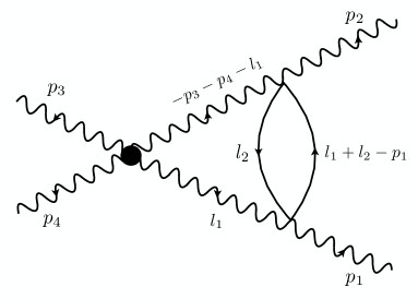
Figure 4: Two-loop correction to the correlator $\langle(\chi_{i}^{2})^{2}(p=0)\chi_{j}(p_{1})\chi_{k}(p_{2})\chi_{l}(p_{3})\chi_{m}(p_{4})\rangle$. The black dot indicates the bare composite operator $(\chi^{2})^{2}$. We also see two $\varphi^{2}\chi^{2}$ vertices. The conventions for the propagators are explained in appendix E.

The susy-null operator with the smallest UV dimension is $(\chi_{i}^{2})^{2}.$ It is the leader operator of the singlet combination $\sigma_{3}\sigma_{1}+\frac{3}{4}\sigma_{2}^{2}$, which is also the Feldman operator $\mathcal{F}_{4}$, see Eq. (8.4). Its anomalous dimension receives no one-loop contribution, while the two-loop correction is given by the diagram in Fig. 4. Using standard techniques (appendix H.2.1) we obtain the IR scaling dimension

$$\Delta_{(\chi_{i}^{2})^{2}}=8-2\varepsilon-\frac{8}{27}\varepsilon^{2}+O(\varepsilon^{3}).$$ (9.7)

Going higher in the UV dimension, we encounter the susy-null leader $\varphi^{2}(\chi_{i}^{2})^{2}$ with classical dimension $10-3\varepsilon$. Since it is the only susy-null leader at this dimension, it does not mix with any other operator. It receives a positive one-loop anomalous dimension equal to $3\varepsilon$, as discussed in appendix H.2.2. We have not evaluated its two-loop anomalous dimension.

At classical dimension $12-3\varepsilon$, we have three susy-null leaders made of six fields, which mix with one another in a nontrivial way: $\varphi\omega(\chi_{i}^{2})^{2},(\chi_{i}^{2})^{3}$ and $(\partial_{\mu}\varphi)^{2}(\chi_{i}^{2})^{2}$. In appendix H.2.3 we compute their anomalous dimension matrix at one loop. As explained there, the matrix is not completely diagonalizable, rather it can be brought to the Jordan form (see also appendix F) with eigenvalues 0 and $(11/9)\varepsilon$, the latter associated to a rank-two Jordan block. In the CFT context, the Jordan block structure of the mixing matrix signals the presence of a logarithmic multiplet, and is a symptom that we are dealing with a logarithmic CFT [40]. This fact is not very surprising since our theory arises from the $n\rightarrow 0$ limit of $S_{n}$-symmetric replica Lagrangian (see [41]).

At classical dimension $12-4\varepsilon$ there is a single composite of eight fields, $\varphi^{4}(\chi_{i}^{2})^{2}$. This also receives a positive one-loop anomalous dimension equal to $(22/3)\varepsilon$, as shown in appendix H.2.4.

We summarize these results in Table 2. As discussed in section 8.5, we count relevant susy-null leaders as possible sources of the SUSY fixed point destabilization. The leader $(\chi_{i}^{2})^{2}$ has the smallest dimension and is one candidate which may cause such a destabilization, once it becomes relevant (see section 10).

Leaders $\mathcal{O}_{\text{null}}$	Full $S_{n}$-singlet perturbation $\mathcal{O}$	IR dimension: $\Delta_{\mathcal{O}_{\text{null}}}$
$(\chi_{i}^{2})^{2}$	$\sigma_{3}\sigma_{1}+\frac{3}{4}\sigma_{2}^{2}$	$8-2\varepsilon-\frac{8}{27}\varepsilon^{2}+O(\varepsilon^{3})$
$\varphi^{2}(\chi_{i}^{2})^{2}$	$\sigma_{2}\sigma_{4}-\frac{8}{5}\sigma_{1}\sigma_{5}$	$10+O(\varepsilon^{2})$
$\varphi\omega(\chi_{i}^{2})^{2}$	$\sigma_{1}\sigma_{2}\sigma_{3}-\frac{3}{2}\sigma_{1}^{2}\sigma_{4}$	$\left.\vphantom{\displaystyle\int\limits_{0}^{\infty}}\right\}\begin{array}[]{c}12-3\varepsilon+O\left(\varepsilon^{2}\right)\\ 12-\frac{16}{9}\varepsilon+O\left(\varepsilon^{2}\right)\end{array}$
$(\chi_{i}^{2})^{3}$	$\sigma_{2}^{3}-2\sigma_{1}\sigma_{2}\sigma_{3}+\sigma_{1}^{2}\sigma_{4}$
$\partial_{\mu}\varphi\partial^{\mu}\varphi(\chi_{i}^{2})^{2}$	$\sigma_{3(\mu)}^{2}-\frac{4}{3}\sigma_{2(\mu)}\sigma_{4(\mu)}+\frac{1}{3}\sigma_{1(\mu)}\sigma_{5(\mu)}$
$\varphi^{4}(\chi_{i}^{2})^{2}$	$\sigma_{2}\sigma_{6}-\frac{12}{7}\sigma_{1}\sigma_{7}$	$12+\frac{10}{3}\varepsilon+O\left(\varepsilon^{2}\right)$

Table 2: Summary of anomalous dimension computations for all susy-null leaders with $\Delta_{\operatorname{UV}}\leqslant 12+O\left(\varepsilon\right)$. For the leaders $\varphi\omega(\chi_{i}^{2})^{2}$, $\varphi\omega(\chi_{i}^{2})^{2}$ and $\partial_{\mu}\varphi\partial^{\mu}\varphi(\chi_{i}^{2})^{2}$ we show the two scaling dimensions arising after mixing (the second one being associated to a rank-two logarithmic multiplet).

Non-susy-writable leaders

In section 8.2, we have identified only one non-susy writable leader up to $\Delta=12$ in $d=6$. It is the leader $(\mathcal{F}_{6})_{L}$ of the Feldman operator $\mathcal{F}_{6}$. Given its expression (8.5) in Cardy fields, its anomalous dimension is studied via the 6-point correlation function $\langle(\mathcal{F}_{6})_{L}(p)\chi_{i}(p_{1})\chi_{j}(p_{2})\chi_{k}(p_{3})\chi_{l}(p_{4})\chi_{m}(p_{5})\chi_{n}(p_{6})\rangle$. Its leading anomalous dimension appears at two loops, from the first diagram in Fig. 15 (see Appendix H.3 for details), and it is negative. The two-loop corrected dimension IR dimension of $(\mathcal{F}_{6})_{L}$ is given by:

$$\Delta_{(\mathcal{F}_{6})_{L}}=12-3\varepsilon-\frac{7}{9}\varepsilon^{2}+O(\varepsilon^{3}).$$ (9.8)

This leader is becoming less irrelevant as $d$ gets smaller, and is another candidate which might destabilize the SUSY RG flow, as we discuss in section 10.

In Appendix H.3 we also considered anomalous dimensions of higher Feldman leaders $(\mathcal{F}_{k})_{L}$, finding at two loops

$$\Delta_{(\mathcal{F}_{k})_{L}}=2k-\frac{k}{2}\varepsilon-\frac{k(3k-4)}{108}\varepsilon^{2}+O(\varepsilon^{3}).$$ (9.9)

This confirms the original result of Feldman [30]. It should be noted that Ref. [30] used the “old” formalism for computing anomalous dimensions, working in the replicated basis with propagator (2.10). The agreement shows that the “old” formalism is not wrong, if one is careful. We believe however that our new formalism (working in the Cardy basis in the vicinity of the Gaussian fixed point, distinguishing leaders and followers, classifying leaders by their symmetry) is more systematic, hence less error prone.

While we confirm Feldman’s result (9.9) for the anomalous dimension, we disagree with his conclusion that this implies instability of the SUSY fixed point for an arbitrary small $\varepsilon$; see section 10.

Scenarios for the loss of SUSY

In the previous sections we carried out the program of classifying the leaders of $S_{n}$ singlet perturbations, and we described many anomalous dimension computations. This is a vast body of knowledge about the spectrum of potentially destabilizing perturbations. On the basis of this information we will now discuss possible scenarios for how SUSY may be lost below a critical dimension $d_{c}$.

The lowest leaders in each of the three classes have dimensions (9.6), (9.7), (9.8). In this section we will use them truncated to the known terms:

susy-writable: $$\Delta_{\mathcal{B}}=10-\frac{11}{9}\varepsilon,$$

susy-null: $$\Delta_{(\chi_{i}^{2})^{2}}=8-2\varepsilon-\frac{8}{27}\varepsilon^{2},$$ (10.1)

non-susy-writable: $$\Delta_{(\mathcal{F}_{6})_{L}}=12-3\varepsilon-\frac{7}{9}\varepsilon^{2}.$$

In Fig. 5 we plot these scaling dimensions as a function of $d$ in the range of interest $3\leqslant d\leqslant 6$. In the same plot we show the marginality threshold line $\Delta=d$.

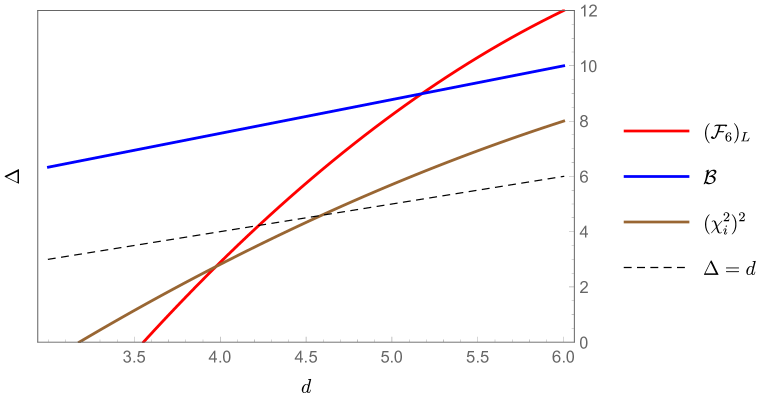
Figure 5: Scaling dimensions of the three lowest leaders (one per each class) as a function of the space dimension $d$, per Eqs. (10.1).

The immediate observation is that $\mathcal{B}$ does not become relevant in this range of $d$, while $(\mathcal{F}_{6})_{L}$ and $(\chi_{i}^{2})^{2}$ do so at:

$$\Delta_{(\chi_{i}^{2})^{2}}=d \quad\operatorname{at}\quad d\approx 4.6,$$

$$\Delta_{(\mathcal{F}_{6})_{L}}=d \quad\operatorname{at}\quad d\approx 4.2.$$

Taking this at face value, SUSY may be lost between $d=4$ and 5 because of these two perturbations.

The first uncertainty in this result is due to the shortness of available perturbative series, which hopefully will be improved in the future by higher-loop computations. E.g., using instead a $\textrm{Pad\'{e}}_{[1,1]}$ rational approximant for the conformal dimensions, we find that $\Delta_{(\chi_{i}^{2})^{2}}$ crosses marginality at $d\approx 4.7$, while $\Delta_{(\mathcal{F}_{6})_{L}}$ at $d\approx 4.5$. This provides a rough idea of this uncertainty.

Another uncertainty is associated with the fact that the coupling of the susy-null $(\chi_{i}^{2})^{2}$, even if relevant, may flow to a nearby fixed point (“small loophole” from section 8.5), in which case SUSY may be preserved. But even if this happens, we still have the non-susy-writable leader $(\mathcal{F}_{6})_{L}$, which will destroy SUSY at a nearby dimension.

Additional uncertainty may be due to the nonperturbative mixing with higher-dimension operators, as we will now discuss.

By nonperturbative mixing we mean the following phenomenon. In perturbation theory, mixing happens between operators of the same symmetry, with additional selection rules that they should have the same number of fields and the same scaling dimension in $d=6$. Beyond perturbation theory, symmetry remains the only selection rule. Let then $\Delta_{1}(d)$ and $\Delta_{2}(d)$ be dimensions of two operators computed in perturbation theory, and suppose these two curves intersect at some $d<6$ (“level crossing”). If these two operators have different symmetry, e.g. belong to different leader classes like in Fig. 5, then the level crossing is allowed also beyond perturbation theory. On the other hand, if the two operators have the same symmetry, then we should not believe the level crossing literally, as it will be modified by nonperturbative mixing effects.

Normally, level crossing will be resolved via level repulsion (Fig. 6, center). Our theory being non-unitary, level crossing may also be resolved via operator dimensions becoming complex conjugate (Fig. 6, right). Which of the two resolutions is realized depends on the sign of the norm of the crossing operators (which is the same as the sign of their two-point functions). Operators whose norm has the same sign will repel (as is always the case in unitary theories), while for the norm of opposite sign, dimension will go into the complex plane. If the mixing operators have zero norm, as in the susy-null case, both options are possible.

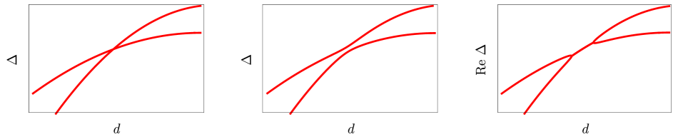
Figure 6: Left: Level crossing for two operator dimensions $\Delta_{1}(d)$, $\Delta_{2}(d)$ of the same symmetry in perturbation theory. Center: Crossing resolved via level repulsion (for norm of the same sign). Right: Crossing resolved via going to the complex plane (for norm of the opposite sign). These plots were obtained by diagonalizing the matrix $\left(\begin{array}[]{cc}\Delta_{1}(d)&p\\ p&\Delta_{2}(d)\end{array}\right)$, where $p$ is a parameter characterizing the nonperturbative mixing strength, taken real or purely imaginary for norms of equal/opposite sign.  

After these general comments, let us see which of the curves in Fig. 5 can be affected by nonperturbative mixing.

The susy-writable leader $\mathcal{B}$ could in principle mix nonperturbatively with other susy-writable leaders coming from the box representations, the first of which is the $10_{2,0\oplus 0,2}$ in Eq. (8.3). The scaling dimension of the corresponding leader $\mathcal{B}^{\prime}$ is:

$$\Delta_{\mathcal{B}^{\prime}}=(12-3\varepsilon)_{\operatorname{class}}+\left(\frac{10}{3}\varepsilon\right)_{\text{1-loop}}+O(\varepsilon^{2})=12+\frac{\varepsilon}{3}+O(\varepsilon^{2}).$$ (10.2)

At $O(\varepsilon)$ the scaling dimension curves do not intersect, and we do not consider this case any further.

The susy-null leader $(\chi_{i}^{2})^{2}$ could in principle mix nonperturbatively with other susy-null leaders shown in Table 2. We plot the perturbative predictions for their scaling dimensions (to known order) in Fig. 7. We see that while the higher curves intersect among themselves, they do not reach the lower $(\chi_{i}^{2})^{2}$ curve.

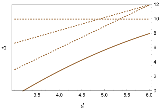
Figure 7: Scaling dimensions of susy-null leaders from Table 2 (known terms).

Finally, the non-susy-writable sector $(\mathcal{F}_{6})_{L}$ may mix nonperturbatively with any of the higher non-susy-writable leaders. We know a part of this higher spectrum, namely the two-loop dimensions of the higher Feldman operators, Eq. (9.9). In Fig. 8 we plot the scaling dimension of the first four $(\mathcal{F}_{k})_{L}$. This time we do see level crossings. In fact, since the 2-loop correction is negative and grows with $k$, it looks like the dimensions of $(\mathcal{F}_{k})_{L}$ intersect the dimensions of all lower $(\mathcal{F}_{k^{\prime}})_{L}$. At least for the first few Feldman operators, these crossings all appear to happen slightly above $d=4$, close to the point where $(\mathcal{F}_{6})_{L}$ becomes relevant.

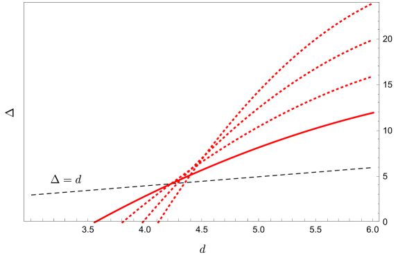
Figure 8: Perturbative scaling dimensions of the leaders of the first four Feldman operators.

This multitude of crossings deserves a discussion. The nonperturbative mixing will likely repel the Feldman operators. As a result the lower Feldman operator will become relevant at a slightly higher $d_{c}$ than without taking mixing into account, while the higher Feldman operators will become relevant at a slightly lower $d$, if at all. SUSY will be valid for $d>d_{c}$. The final picture may perhaps resemble that of Fig. 9. This deserves further study, but we emphasize that any future discussion of this problem should take nonperturbative mixing into account. It should also be remembered that Feldman operators are but a small subset of all the non-susy-writable operators which can be expected to take part in this mixing, see section H.3.

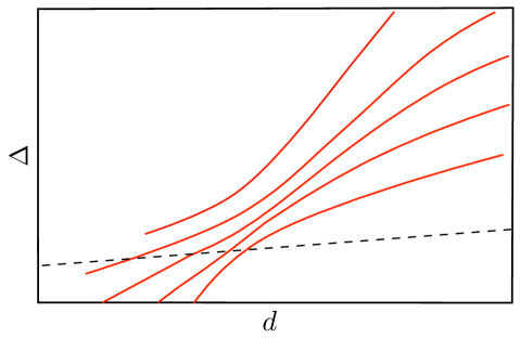
Figure 9: Schematic dimension curves for Feldman operators after taking nonperturbative mixing into account. In making this figure we assumed the simplest scenario that all Feldman operators have the norm of the same sign and hence repel each other rather than go into the complex plane. It would be interesting to verify the norm sign in the future. For this one would have to determine the eigenperturbations and compute the sign of the two-point functions. This plot also does not take into account that there exist other non-susy-writable operators, with which higher Feldman operators are expected to mix beyond two-loop order, see section H.3.

Finally we would like to discuss what would happen if one naively extrapolated Fig. 8 to extremely high $k$. The two-loop result Eq. (9.9) would seem to predict that $(\mathcal{F}_{k})_{L}$ becomes relevant for $\varepsilon_{c}\sim\sqrt{72/k}$ which goes to zero for $k\rightarrow\infty$. This was the argument advanced by Feldman [30], who thus concluded that arbitrarily close to $d=6$ there will be some sufficiently high $(\mathcal{F}_{k})_{L}$ which is already relevant. Hence, he argued, SUSY will be not present at any $d<6$. We do not trust this argument for two reasons. First, because it ignores nonperturbative mixing discussed above. Second, because to have $\varepsilon_{c}$ small we would have to consider very large $k$ indeed. E.g. for $k=50$ we still have $\varepsilon_{c}=1.01$ from the two-loop result. On the other hand the coefficients of the perturbative series grow with $k$, as already visible in (9.9). Therefore the two-loop prediction at very large $k$ will be trustworthy only in a tiny range of $\varepsilon$, and cannot by itself be used to find where $(\mathcal{F}_{k})_{L}$ becomes relevant and if this happens at all. For these reasons, we do not think it likely that infinitely many Feldman operators will cross or approach the relevance threshold.

To summarize, our computations suggest that Parisi-Sourlas SUSY will be lost below a critical dimension $d_{c}\approx 4.2$ - $4.7$. Around this dimension, SUSY-breaking perturbations from two different symmetry sectors (susy-null and non-susy-writable leaders) become relevant. In particular, for integer dimension 5 all perturbations are irrelevant and Parisi-Sourlas SUSY is expected to be present. For integer dimension 4, one perturbation with a susy-null leader and at least one non-susy-writable perturbations are relevant, and the RG flow is directed away from the SUSY fixed point. The phase transition in the 4d RFIM is therefore not expected to be supersymmetric.

Discussion

In this paper we laid out a comprehensive framework to study RG stability of the Parisi-Sourlas supersymmetric fixed point describing the phase transition in the Random Field Ising Model. The key ingredients of our approach are:

• We used the Cardy-transformed basis of fields $\varphi,\omega,\chi_{i}$, in which the RG flow looks manifestly as a Gaussian fixed point perturbed by a weakly-relevant interaction near the upper critical dimension 6.

• We decomposed $S_{n}$-invariant perturbations (in the Cardy basis) into the leaders and followers. Scaling dimension of the leader then determines whether the whole perturbation is relevant.

• We classified the leaders into three classes by their symmetry (susy-writable, susy-null, and non-susy-writable).

• Susy-writable leaders were additionally classified as belonging to superprimary multiplets transforming in particular $\operatorname{OSp}(d|2)$ representations.

• We enumerated all leaders up to 6d dimension $\Delta=12$, and computed their perturbative anomalous dimensions (at one or two loops).

On the basis of the above, we identified two $S_{n}$-invariant perturbations which become relevant at a critical dimension $d_{c}$ slightly above 4. In the replicated field basis $\phi_{i}$, these perturbations correspond to $\mathcal{F}_{4}$ and $\mathcal{F}_{6}$, where $\mathcal{F}_{k}=\sum_{i,j=1}^{n}(\phi_{i}-\phi_{j})^{k}$ is the series of operators considered long ago by Feldman [30]. Although looking similar in the replicated basis, in our picture the two perturbations belong to two different classes: $\mathcal{F}_{4}$ has a susy-null leader $(\chi_{i}^{2})^{2}$, while $\mathcal{F}_{6}$ has a non-susy-writable leader.

The above conclusions were based on perturbative calculations of anomalous dimensions around 6d, and on considering the lowest leaders in each class. In the non-susy-writable class, perturbative calculations indicate level crossing between $\mathcal{F}_{6}$ and the higher Feldman operators $\mathcal{F}_{k}$, $k>6$. We discussed how this level crossing is expected to be resolved by nonperturbative mixing effects, pushing slightly up the critical dimension $d_{c}$ at which $\mathcal{F}_{6}$ will become relevant.

To summarize, the main features of our scenario for the loss of SUSY are:

1. SUSY fixed point exists for any $3<d\leqslant 6$.

2. SUSY fixed point is stable for $d>d_{c}$ and unstable for $d<d_{c}$, where $d_{c}\approx 4.2$ - $4.7$.

Our scenario is therefore different from the loss of SUSY in any $d<6$ advocated for various reasons in some works such as [49, 50, 28, 30]. It is also different from the disappearance of the SUSY fixed point via fixed point annihilation, found in Functional Renormalization Group (FRG) studies [23, 51, 52, 53, 54] at $d_{c}\approx 5.1$ (see App. A.7). For them, SUSY is absent for $d<d_{c}$ because there is no longer any SUSY fixed point, while for us the SUSY fixed point exists for any $d$, it just becomes unstable for $d<d_{c}$. [The value of $d_{c}$ is also different but this is less important.] We do not see any signs of fixed point annihilation in our picture. For us, this would require that a SUSY-preserving operator crosses the relevance threshold. In the language of section 9.1, this would be a scalar $\mathbb{Z}_{2}$-even susy-writable leader, and as discussed there all such operators remain irrelevant for all $d$.

Our work suggests two kinds of open problems: to explore our method further, and to check our conclusions with other techniques. We discuss these in turn.

Exploring our method further

Symmetry meaning of leaders in the Cardy basis

One aspect of our construction which deserves further thinking is the symmetry understanding of leaders. Leaders were introduced as the lowest-dimension components of $S_{n}$-singlet operators. We then argued (and checked extensively) that leaders only mix with leaders under RG. If so there must be a symmetry reason for this fact contained in the $\mathcal{L}_{0}$ Lagrangian (without appealing to the original $S_{n}$ invariant Lagrangian), and it would be interesting to identify such a reason. For susy-writable leaders we gave a criterion (section 8.3) that they become supertranslation invariant when written in the SUSY field basis, and it would be interesting to prove this more rigorously.

Another hint for such a symmetry may come from an interesting property which all leader operators have: their correlation functions vanish. One easy argument for this comes from considering correlation functions of $S_{n}$-singlets written in terms of the original replicated fields $\phi_{i}$ (namely without writing them in Cardy basis). It is indeed easy to prove that such correlation functions are proportional to $n$ and thus vanish in the $n\to 0$ limit. [This is related to the fact that the partition function of replicated theory is exactly 1 in the $n\to 0$ limit.] As an example let us consider $\langle\sigma_{k_{1}}\dots\sigma_{k_{m}}\rangle$ in the free replicated theory (namely (2.7) with $V=0$). The result of this correlator can be written as a product of propagators (2.10), thus it is proportional to the trace of a product of the matrices $\mathds{1}$ and ${\mathbf{M}}$ of (2.10). Since $\mathrm{tr}(\mathds{1}\cdots\mathds{1}\mathbf{M}\cdots\mathbf{M})=O(n^{a})$ with $a\geqslant 1$, the result must vanish as $n\to 0$. This argument generalizes straightforwardly for more generic $S_{n}$ singlets and it is also easy to see that when $V\neq 0$, at any order in perturbation theory, the same property must hold, since the potential is also an $S_{n}$-singlet by construction. We thus conclude that correlation functions of $S_{n}$-singlets vanish. Since the leaders are lowest dimensional pieces of $S_{n}$-singlets, their correlators must vanish too.

But can we understand this vanishing of correlators directly in terms of leaders, without appealing to $S_{n}$-singlets from which the leaders originated? For susy-writable leaders we can, since they are the highest component of a supermultiplet, so, by supersymmetry, their correlation function must be zero (this is the same arguments that predicts $\langle\omega(x)\omega(0)\rangle=0$). Also correlation functions of susy-null leaders must vanish, since the operator are null (similarly this happens for mixed correlation functions of susy-null operators and susy-writable ones). A less trivial case is when non-susy-writable leaders are inserted in the correlation function. In this case SUSY arguments don’t apply, and one has to find a new strategy to prove the statement.

Higher-loop computations

Perturbative computations of anomalous dimensions played an important role in our considerations. In this work we relied on one- and two-loop predictions. In comparison, 6- or 7-loop results are available nowadays for the leading critical exponents in the Wilson-Fisher $4-\varepsilon$ expansion [55, 56]. It would be interesting to compute higher loop anomalous dimensions of composite operators responsible for destabilizing the SUSY fixed point. Resumming these series could lead to improved determinations of $d_{c}$.

Branched polymers and the Lee-Yang universality class

One can consider the same problem as we studied in this paper, but replacing the quartic potential $\phi^{4}$ with the imaginary cubic potential $i\phi^{3}$ [18, 19]. As mentioned in section 1 and reviewed in App. A.4, this “Random Field Lee-Yang Model”, with upper critical dimension 8, describes the phase transition in the system of random polymers. Dimensional reduction from $d$ to $d-2$ dimensions in this case is verified to high precision by Monte Carlo simulations. Therefore, we do not expect to find instability phenomena that we found here for the RFIM case. In other words, leader anomalous dimensions in the $i\phi^{3}$ theory should be such that they will not cross the relevance threshold. It would be very interesting to verify this explicitly. Note that both $\mathbb{Z}_{2}$ invariant and $\mathbb{Z}_{2}$ breaking leaders should be considered in this computation, since $\mathbb{Z}_{2}$ is not a symmetry of the Lee-Yang model.

Checking our conclusions with other techniques

Numerical simulations

A feature of our scenario is that the Parisi-Sourlas SUSY fixed point exists in any $d>3$ (although it becomes unstable for $d<d_{c}$). In principle, this could be tested in numerical lattice simulations. State-of-the-art simulations study the RFIM phase transition at zero temperature, by tuning the disorder distribution. In practice one considers a one-parameter family of distributions with a fixed shape and varying overall strength (i.e. dispersion). E.g. Ref. [7] did this in $d=4$ for the Gaussian and Poisson disorders. In both cases they found identical, non-SUSY, critical exponents (as reviewed in App. A.2). If the SUSY fixed point exists in $d=4$, it should be possible to observe it by tuning within a family of disorder distributions depending on a larger number of parameters (as many as there are relevant perturbations at the SUSY fixed point). As discussed in section 10, it looks like at least two more perturbations in addition to the SUSY mass become relevant in $d=4$ ($\mathcal{F}_{4}$ and $\mathcal{F}_{6}$). If that is the case, one would have to consider a 3-parameter family of distributions to find a SUSY fixed point in a lattice simulation—a daunting task. But perhaps the higher-loop terms slightly modify the behavior of anomalous dimensions on $d$, and only one extra perturbation becomes relevant in $d=4$, so that a 2-parameter family would suffice. See App. I for a schematic discussion of this possibility.

Another question is whether one can measure some of the observables considered in this paper through a lattice simulation, e.g. in $d=5$, where the SUSY fixed point is expected to be reached. In particular it would be interesting to compute the scaling dimensions of the leaders of the $S_{n}$-singlet operators $\mathcal{F}_{4}$ and $\mathcal{F}_{6}$ and check that these are indeed irrelevant in $d=5$. Let us explain how this can be done. Any correlation function of any operator in Cardy variables can be mapped to a correlator of the random field theory by first rewriting it in terms of the replicated fields $\phi_{i}$ following Eqs. (2.11),(2.14) and then by using the recipe in Eqs. (2.6),(2.8). An example of such computation is done in (2.32-2.34) and (38), but it can be easily generalized to any kind of operator, in particular to the leaders of $\mathcal{F}_{4}$ and $\mathcal{F}_{6}$. It is however important to mention that correlation functions of both $S_{n}$-singlets and of their leaders are vanishing as we explain in section 11.1.1. Hence one cannot extract the dimension of a leader by computing its two point function, since this would be zero. One should consider instead more complicated correlation functions involving non-singlet operators. E.g. $\Delta_{(\mathcal{F}_{6})_{L}}$ can be studied with the help of the 3-point function $\langle(\mathcal{F}_{6})_{L}(x_{1})\varphi(x_{2})\varphi(x_{3})\rangle$. On the other hand, the susy-null dimension $\Delta_{(\mathcal{F}_{4})_{L}}$ may be accessible via through a 3-point function $\langle(\mathcal{F}_{4})_{L}(x_{1})\mathcal{O}(x_{2})\mathcal{O}(x_{3})\rangle$, where $\mathcal{O}$ has to be non-singlet and in addition non-susy-writable, otherwise the result will vanish. These kind of observables would be very interesting to study. Even if higher point functions are significantly more complicated to compute in a lattice simulation, we hope that progress can be done in this direction. E.g. the same scaling dimensions $\Delta_{(\mathcal{F}_{6})_{L}}$ and $\Delta_{(\mathcal{F}_{4})_{L}}$ can be extracted from finite-volume corrections to scaling of the two point functions $\langle\varphi\varphi\rangle$ and $\langle\mathcal{O}\mathcal{O}\rangle$.

Conformal bootstrap

In recent years, the conformal bootstrap has emerged as a powerful method to study nonperturbative CFTs in any dimension (see the review [58]). Most of its successes have been for unitary CFTs, which can be analyzed rigorously due to the unitarity bounds for the operator dimensions and reality constraints on the OPE coefficients, as was first shown in [59]. These rigorous methods do not directly apply to the Parisi-Sourlas SUSY fixed point which is non-unitary, as visible e.g. in $\Delta_{\varphi}$ below the scalar unitarity bound, and in the violation of spin-statistics by spinless fermions.

Scaling dimensions of susy-writable leaders could be obtained by looking at the corresponding primaries in the Wilson-Fisher fixed point in $\widehat{d}=d-2$ dimensions. This is complicated by the fact that in integer $d$ some interesting representations project to zero, while for non-integer $d$ the Wilson-Fisher theory is also non-unitary [37] (as already mentioned in section 9.1). For us, the most interesting susy-writable leader is the box operator $\mathcal{B}$, whose dimension equals that of the Wilson-Fisher box primary $\widehat{B}$. The number of components ($O(\widehat{d})$ irrep dimension) of $\widehat{B}$ is given by (see Eq. (H.4)) $\dim(\widehat{B})=\frac{(\widehat{d}+2)(\widehat{d}+1)\widehat{d}(\widehat{d}-3)}{12}.$ We have  $\dim(\widehat{B})=10$ for $\widehat{d}=4$ consistently with box=$(2,0)\oplus(0,2)$ in that dimension. Note that $\dim(\widehat{B})$ vanishes for $\widehat{d}=3$, which means that $\widehat{B}$ does not exist in 3d, i.e. $\mathcal{B}$ projects to zero under dimensional reduction from $d=5$ to 3. For $3<\widehat{d}<4$, $\dim(\widehat{B})$ is positive. Perhaps in this range of $\widehat{d}$ some trustworthy, albeit non-rigorous, information about the scaling dimension of $\widehat{B}$ can be provided by the standard numerical bootstrap (applying it e.g. to the 4-point functions of spin-one operators or stress tensors).

Apart from the lack of positivity, there are other complications in applying the conformal bootstrap method to the RFIM. First, the fixed point of interest exists only for $n=0$, thus precluding the analytic continuation of CFT data in $n$ (section 6). Second, the CFT is expected to contain logarithmic multiplets (section 9.2), for which logarithmic conformal blocks need to be used instead of the usual conformal blocks [40].

At present, the only bootstrap algorithm not relying on positivity and thus applicable also to non-unitary CFTs is the one proposed by Gliozzi [63]. In its present incarnation this algorithm is not rigorous, as well as less systematic than the standard numerical bootstrap algorithms. In spite of the lack of rigor and the above-mentioned complications, it would be interesting to try to apply Gliozzi’s algorithm to the RFIM fixed point. This was attempted by Hikami [66], who found support for the loss of dimensional reduction below $d_{c}\approx 5$. As we explain in App. A.10, more work in this direction is needed to verify the robustness of Hikami’s results and to extract what they say about the mechanism for the loss of dimensional reduction.

Functional renormalization group

Previous functional renormalization group (FRG) studies of the RFIM phase transition, such [23, 51, 52, 53, 54] (see App. A.7) used the $S_{n}$-symmetric formalism. In principle, it should also be possible to apply the FRG method in the Cardy field basis. For that one would have to package an infinite series of singlet operators in a general function. E.g., one could generalize Feldman operators to an $S_{n}$-invariant interaction parametrized by a general function $R$:

$$\sum_{i,j=1}^{n}R(\phi_{i}-\phi_{j}),$$ (11.1)

which in the Cardy basis becomes

$$2\sum_{i=2}^{n}R(\omega-\chi_{i})+\sum_{i,j=2}^{n}R(\chi_{i}-\chi_{j}).$$ (11.2)

[Separating it into a leader plus followers may not be necessary in a nonperturbative framework such as FRG.] One could then derive an RG flow equation for the function $R$, leading to the anomalous dimension predictions for the Feldman operators. Note that this RG equation will be different from that in the FRG studies of the interface disorder (section A.6), because of the presence of the quartic coupling in our problem. Also unlike in section A.6, the function $R$ for us does not have to satisfy any conditions at infinity. It would be interesting to carry out this exercise, as a way to confirm our expectations from section 10 about the mixing and level repulsion of these operators.

Appendix A History and prior work

Early work

That critical exponents of random-field $\phi^{4}$ theory in $d=6-\varepsilon$ agree with Wilson-Fisher in $d=4-\varepsilon$ was first proved by Aharony, Imry and Ma in 1976 [67] (see also Young [68]). They picked out a subclass of perturbative diagrams most divergent in IR, and showed them identical to those of the Wilson-Fisher theory with coupling $\lambda^{\prime}=\lambda H$, for $(d-2)$-dimensional external momenta.

Parisi and Sourlas [5] rephrased this calculation in terms of supersymmetry. The diagrams in question being tree-level in $\phi$ (before integrating over the random field), their sum can be done by solving the classical equation of motion in external field $h$. This can be then neatly interpreted as a path integral with insertion $\delta(-\Delta\phi+V^{\prime}(\phi)-h)\det(-\Delta+V^{\prime\prime}(\phi))$. Introducing a Lagrange multiplier field $\omega$ for the $\delta$-function and a pair of anticommuting scalars to represent the determinant, one lands on a supersymmetric action. Dimensional reduction is then argued in perturbation theory using superpropagators and the identity $\int d^{d-2}x\,F(Y_{i}x,x^{2})=\int d^{d}xd\theta d\bar{\theta}\,F(Y_{i}x,x^{2}+\bar{\theta}\theta)$ where $Y_{i}$ are $d-2$ dimensional vectors. The position space argument is thus easier than the momentum space one.

No SUSY and no dimensional reduction in $d=3,4$

The Parisi-Sourlas conjecture fails in $d=3$: the $d=3$ RFIM is ordered at low temperatures (for weak disorder) by the Imry-Ma criterion [69], while $d=1$ Ising is of course disordered at all temperatures and does not even have a phase transition. The ordering of 3d RFIM was also proved rigorously by Imbrie [70, 71] ($T=0$) and by Bricmont and Kupiainen [72, 73] (small $T$).

The transition is believed continuous in 3d. Numerical simulations can be done at $T=0$ varying the disorder strength to reach the transition. One uses fast algorithms to find exact ground states for a collection of disorder samples, and then performs disorder average. In this setup, a large-scale study on cubic lattices with size up to $L=192$ and with $10^{7}$ disorder samples was performed by Fytas and Martin-Mayor [6]. They found a continuous transition with exponents $\nu\approx 1.4(1)$, $\eta\approx 0.515(1)$. Defining different exponents for the connected and disconnected propagators as

$$\overline{\partial\langle S_{x}\rangle/\partial h_{y}}\sim 1/r^{d-2+\eta},\quad\overline{\langle S_{x}\rangle\langle S_{y}\rangle}\sim 1/r^{d-4+\bar{\eta}}$$ (A.1)

they find $\bar{\eta}\approx 2\eta$. SUSY is ruled out as it would predict $\bar{\eta}=\eta$. Correction to scaling exponent is  $\omega=0.52(11)$.

The $d=4$ RFIM and $d=2$ Ising both have a phase transition but exponents do not agree. The $d=4$ RFIM exponents were measured precisely in [7], with results $\nu\approx 0.872(6)$, $\eta\approx 0.1930(13)$,  $2\eta-\bar{\eta}\approx 0.032(2)$, $\omega\approx 1.3(1)$. In particular $\bar{\eta}\neq\eta$ and SUSY is ruled out.

SUSY in $d=5?$

The $d=5$ RFIM study [8] found $\nu=0.626(18)$, $\eta=0.055(15)$, $2\eta-\bar{\eta}=0.058(8)$, $\omega=0.66(15)$. Within error bars, this is largely consistent with both SUSY $\bar{\eta}=\eta$ and with the 3d Ising exponents ($\nu=0.629971(4)$, $\eta=0.036298(2)$, $\omega=0.82966(9)$ from the conformal bootstrap [74, 75]).

Further evidence for SUSY and dimensional reduction in 5d RFIM was presented in [9], which simulated elongated hypercube geometries with $d-2$ dimensions fixed at $L$ and 2 remaining ones at $RL$. For $R\rightarrow\infty$ and $L$ fixed, SUSY imposes relations between connected and disconnected propagators, and these relations were found to be satisfied in $d=5$ (working at $R=5$). E.g. three independent finite-volume correlation lengths (which scale with $L$) were found equal at a percent level: for the connected and disconnected propagators in 5d RFIM and for the 3d Ising.

Branched polymers and the Lee-Yang universality class

Another interesting case of dimensional reduction occurs for the statistics of branched polymers which can be modeled as connected clusters of $N$ points on a lattice (“lattice animals”). Their number $P(N)$ and average size $R$ scales as $P(N)\sim N^{-\theta}\lambda^{N}$, $R\sim N^{\nu}$ where $\theta,\nu$ are critical exponents and $\lambda$ is a lattice-dependent non-universal constant. Lubensky and Isaacson [76] proposed a field-theoretic description for extracting these exponents from a scalar theory in $n\rightarrow 0$ limit, similar to de Gennes’s description of self-avoiding walks but with extra cubic vertices breaking $O(n)$ symmetry to $S_{n}$. Parisi and Sourlas [77] then interpreted this as the replica method limit for the random field model (1.4) with the cubic potential $V(\phi)=m^{2}\phi^{2}+ig\phi^{3}$. Via supersymmetry, critical exponents should be the same as for the Lee-Yang universality class in $d-2$ dimensions. The lattice animals exponents are known from precise Monte Carlo simulations [78] for all $d<d_{uc}=8$ and indeed they agree with the Lee-Yang exponents (known exactly or approximately depending on $d$).

Brydges and Imbrie [57] found a model of branched polymers which has manifest supersymmetry at the microscopic level (see also review [79]). In their model branched polymers are represented as a gas of particles in $d$ dimensions with weight $\prod_{i\sim j}Q(r^{2}_{ij})\prod_{i\nsim j}P(r_{ij}^{2})$ where $Q$ keeps neighboring nodes at a distance $r\sim a$ apart, while $P$ repels all other nodes. Supersymmetry is present if $Q(x)=dP(x)/dx$. In this case, the model can be written as a classical gas of particles in $\mathbb{R}^{d|2}$ interacting with repulsive potential $V$, $e^{-V}=P$. Dimensional reduction follows, to a classical repulsive gas in $\mathbb{R}^{d-2}$. The latter model has a critical point at negative fugacity which is one of two famous microscopic realizations of the Lee-Yang universality class [80, 81] (the other being the Ising model in imaginary magnetic field [82]). Brydges and Imbrie’s result is limited to their model of polymers and to the finetuned case of $Q=P^{\prime}$. It does not explain why supersymmetry should emerge in a generic model of branched polymers (i.e. why supersymmetry breaking deformations are irrelevant). This explanation may come from repeating the analysis of our paper for the cubic potential (see section 11.1.3).

Zero-temperature fixed points

Long-distance behavior of disordered systems is often described in terms of “zero-temperature fixed points”. Some features of these fixed points appeared to us rather unusual, and we will attempt here a review for non-expert audience, according to our own incomplete understanding. We found particularly useful the original references [83, 84], and section 8.5 of [31].

To set the notation, recall that the usual “fixed point” is a system with an action $S(\{\phi\},\{\lambda\})$ depending on a collection of fields $\{\phi\}$ and couplings $\{\lambda\}$, which remains invariant under an RG transformation corresponding to the RG change of scale $x^{\prime}=bx$, $b>1$, in the sense that all couplings are invariant: $\{\lambda^{\prime}\}=\{\lambda\}$. To exhibit this invariance one may have to reparametrize the fields after performing RG transformation (e.g. rescale them). One of the RG invariant couplings may be taken to be temperature itself. E.g., the fixed point describing the ferromagnetic phase transition in the usual, non-disordered Ising model has a fixed nearest-neighbor coupling $J$ which can be identified also with the inverse temperature, as well as infinitely many other couplings corresponding to the next-to-nearest and other possible $\mathbb{Z}_{2}$ invariant couplings, which may be neglected in an approximate treatment.

In the same notation, by a “zero-temperature fixed point” one means a system whose action is written with an explicit $T^{-1}$ factor, $\frac{1}{T}S(\{\phi\},\{\lambda\})$, and whose behavior under RG amounts to the change $T^{\prime}=b^{-\theta}T$ with $\theta>0$ a critical exponent, while all the other couplings $\{\lambda\}$ remain invariant. So $T\rightarrow 0$ as one iterates RG. Two well-known examples are the low-temperature fixed points describing the ordered phase of the Ising model, as well as of the $O(N)$ model with $N>2$, $d\geqslant 3$. Both of these cases lead to simple long-range behavior (gapped for Ising, Gaussian with massless Goldstones for $O(N)$).

What is unusual is that disordered phase transition are often described by non-Gaussian zero-temperature fixed points. RFIM is one example. Rewriting the Hamiltonian (1.1) as $\frac{1}{T}\Bigl{[}-\sum_{\langle ij\rangle}s_{i}s_{j}+\sum_{i}h_{i}s_{i}\Bigr{]}$, $\overline{h_{i}^{2}}=\Delta^{2}$, the $d>2$ phase diagram in the space $(T,\Delta)$ is shown in Fig. 10. It contains the usual non-disordered fixed point at $T=T_{c}$ which is unstable under arbitrarily small disorder (Harris criterion) and flows to the disordered fixed point at $T=0$, $\Delta=\Delta_{c}$. This fixed point is a zero temperature fixed point according to the above definition. The critical exponent $\theta$ is known to be 2 in $d=6-\varepsilon$ to all orders, while $\theta=1+\varepsilon/2$ for $d=2+\varepsilon$ [83].

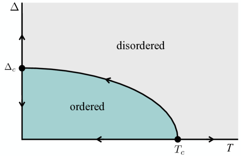
Figure 10: Phase diagram of the RFIM for $d>2$.

Physically, this means that the thermal fluctuations are negligible to those due to disorder at the phase transition. This is very useful in numerical simulations of the RFIM phase transition as it can be done at zero temperature with $\Delta=\Delta_{c}$. One picks a large ensemble of disorder representatives $\{h_{i}\}$, for each of these one computes the ground state (the configuration of spins with minimal energy $-\sum_{\langle ij\rangle}s_{i}s_{j}+\sum_{i}h_{i}s_{i}$). This can be done in polynomial time with the push-relabel algorithm [85], the solution is generically unique, and the critical slow-down is not too bad [86, 87]. These zero-temperature algorithms are used in modern large scale numerical simulations [6, 7, 8, 9].

Let us discuss how the zero-temperature fixed point concept is reconciled with perturbation theory in $d=6-\varepsilon$ and Parisi-Sourlas SUSY ([84] and [31], section 8.5). Consider the replicated action (2.7). Restoring the temperature dependence, the Lagrangian takes the form $\frac{1}{T}\sum_{i=1}^{n}\frac{1}{2}(\partial_{\mu}\phi_{i})^{2}+\lambda_{0}\phi^{4}_{i}-\frac{H_{0}}{2T^{2}}\left(\sum_{i=1}^{n}\phi_{i}\right)^{2}$ where $\overline{h(x)h(x^{\prime})}=H_{0}\delta(x-x^{\prime})$. Rescaling the fields we get the action as in (2.7) with $\lambda=T\lambda_{0}$, $H=H_{0}/T$. If we use the classical scalar dimension in 6d, then an RG step with rescaling factor $b>1$ will give $\lambda^{\prime}=b^{-2}\lambda$, $H^{\prime}=b^{2}H$. We see that this corresponds to $\lambda_{0},H_{0}$ being invariant, while $T^{\prime}=T/b^{2}$, so we flow to a zero-temperature fixed point $(\theta=2)$.

Let us next consider $d<6$ and connect with the Cardy-transformed description. In the basic scenario of section 2.4, the IR fixed point is described by the Lagrangian (2.21) with $H$ and the quartic $\lambda$ both RG-invariant, provided that the fields $f\in\{\varphi^{\prime},\chi_{i}^{\prime},\omega^{\prime}\}$ are rescaled by $f^{\prime}(x)=b^{\Delta_{f}}f(bx)$ where $\Delta_{\chi}=\Delta_{\varphi}+1$, $\Delta_{\omega}=\Delta_{\varphi}+2$. If on the other hand we do the rescaling using $\Delta_{\chi}$ instead of $\Delta_{f}$ for all three fields, the Lagrangian will retain its form with the unit-normalized kinetic terms, but $H,\lambda$ will change as $H^{\prime}=b^{2}H$, $\lambda^{\prime}=\lambda/b^{2}$, which as we have seen above is equivalent to a zero-temperature fixed point. We conclude that $\theta=2$ in any $d<6$ where Parisi-Sourlas SUSY holds.

We thus see that the zero-temperature fixed point can manifest itself in many guises. In lattice simulations we can just set $T=0$. On the other hand, in the standard replicated description (2.7) we are forced to keep $T\neq 0$ even though it flows to zero (a coupling which flows to zero but cannot be simply dropped is “dangerously irrelevant”, footnote 32). Alternatively, we are forced to keep the quartic coupling $\lambda_{0}$ in the action although it is irrelevant and flows to zero, because it combines with another coupling $H_{0}$ which flows to infinity. Finally, in the Cardy field basis the zero-temperature fixed point looks like the usual non-zero temperature one: nothing flows to zero or infinity provided that we use the correct dimensions of fields in the SUSY multiplet. The latter property is of course the chief reason why we used the Cardy basis throughout this paper.

But what if we decide, for the sake of the argument, to forego RG and set $T=0$ directly in the Landau-Ginzburg description (1.4)? This would mean that we have to find, for each random $h(x)$, the field $\phi_{h}$ solving the classical EOM

$$-\partial^{2}\phi_{h}+V^{\prime}(\phi_{h})+h=0,$$ (A.2)

and having the minimal energy. This gives in fact the fastest way to “derive” Parisi-Sourlas SUSY. We represent the resulting path integral as

$$\int\mathcal{D}\phi\,\delta(\phi-\phi_{h})\mathcal{P}(h)\mathcal{D}h=\int\mathcal{D}\phi\,\mathcal{P}(h)\mathcal{D}h\,\delta(-\partial^{2}\phi+V^{\prime}(\phi)+h)\det(-\partial^{2}+V^{\prime\prime}(\phi)).$$ (A.3)

where we reexpressed $\delta(\phi-\phi_{h})$ assuming the solution of (A.2) is unique. We can further rewrite this as

$$\int\mathcal{D}\varphi\mathcal{D}\omega\mathcal{D}\psi\mathcal{D}\bar{\psi}\mathcal{P}(h)\mathcal{D}h\,e^{\int\omega(-\partial^{2}\phi+V^{\prime}(\phi)+h)+\int\psi(-\partial^{2}+V^{\prime\prime}(\varphi))\bar{\psi}},$$ (A.4)

and upon averaging over Gaussian $h$ we land on the SUSY Lagrangian. This was in fact the derivation used originally by Parisi and Sourlas [5] except that they argued the localization to solutions of (A.2) based on the structure of most important terms in perturbation theory, not on the fact that the fixed point is at zero temperature. In retrospect, their argument proves that fixed point is at zero temperature in perturbation theory [84].

By convexity arguments, Eq. (A.2) has a unique solution for any $h$ as long as $m^{2}\geqslant 0$. At the same time, for $m^{2}<0$ there are multiple solutions for some $h$. This is discussed in Parisi’s Les Houches 1982 lectures [49] (see also [88, 89]). The bare mass at the phase transition is expected to be negative, and so multiple solutions are always present at the short-distance scale. In presence of multiple solutions, Parisi-Sourlas path integral (A.4) can be reduced to the sum over all solutions weighted by the determinant. This deviates from what one originally wanted: just the minimal energy solution. One can try to relate this deviation to nonperturbative effects, which may lead to exponentially small $e^{-C/\varepsilon}$ deviations from dimensional reduction already in $d=6-\varepsilon$ [49, 50]. It appears that the constant $C$ has never been computed, which makes the reality of these corrections somewhat nebulous. In fact, multiple solutions may be a short-distance phenomenon, their effect renormalized away when one flows to long distances. To see whether this scenario is realized, one may wish to study the whole RG flow leading to the zero-temperature fixed point and see if the RG fixed point is stable (rather than set $T=0$ from the start). That is exactly what we did in the main text of the paper.

Interface disorder

Another famous occurrence of disorder is in statistical physics of interfaces (see e.g. lecture notes by Kay Wiese [90] and by Leon Balents [91]). Some aspects of this problem are analogous to RFIM, although there are also differences because the symmetry is not the same.

An interface is a scalar function $u(x)$, $x\in\mathbb{R}^{d}$, described by an action

$$\frac{1}{T}\int d^{d}x\left[\frac{1}{2}(\partial u)^{2}+V(x,u(x))\right],$$ (A.5)

where $V$ is a random potential. [E.g. one may imagine the interface between two phases of $d+1$ dimensional Ising model at $T<T_{c}$, the disorder potential $V$ coming from impurities.] We kept $T$ explicit in the action. The potential is taken Gaussian random with

$$\overline{V(x,u)}=0,\quad\overline{V(x,u)V(x^{\prime},u^{\prime})}=\delta^{d}(x-x^{\prime})R(u-u^{\prime}).$$ (A.6)

As a consequence of the shift symmetry $u\rightarrow u+\operatorname{const}$, the variance depends on the difference $R(u-u^{\prime})$, assumed an even function. One is interested in computing various correlators of $u(x)$, e.g.

$$\overline{(\langle u(x)\rangle-\langle u(y)\rangle)^{2}}\sim|x-y|^{2\zeta}$$ (A.7)

at long distances, where $\zeta$ is called the roughness exponent .

Replica method then leads to the Lagrangian:

$$\frac{1}{T}\sum_{i}\frac{1}{2}(\partial u_{i})^{2}-\frac{1}{2T^{2}}\sum_{ij}R(u_{i}(x)-u_{j}(x)).$$ (A.8)

Compared to the RFIM replicated Lagrangian (2.7) (with $\phi_{i}\leftrightarrow u_{i}$), this Lagrangian lacks the individual potential $V(u_{i})$ which is forbidden by the shift symmetry. The term $\left(\sum_{i}u_{i}\right)^{2}$ is reproduced for the quadratic $R(u)$, because $\sum_{ij}(u_{i}-u_{j})^{2}=-2\sum_{ij}u_{i}u_{j}=-2\left(\sum u_{i}\right)^{2}$ in the $n\rightarrow 0$ limit. For $R(u)=u^{k}$, the perturbation in (A.8) is nothing but the Feldman operator $\mathcal{F}_{k}$ which played such an important role in our paper. Applying the Cardy transform $u_{1}=\varphi+\omega/2$, $u_{i}=\varphi-\omega/2+\chi_{i}$ $\left(i=2,\ldots,n,\sum\chi_{i}=0\right)$ gives, in the $n\rightarrow 0$ limit, the Lagrangian

$$\frac{1}{T}\left[\partial\varphi\partial\omega+\frac{1}{2}\sum(\partial\chi_{i})^{2}\right]+\frac{R^{\prime\prime}(0)}{2T^{2}}\omega^{2}-$$

$$\quad-\frac{R^{(4)}(0)}{8T^{2}}\left[\left(\sum\chi_{i}^{2}\right)^{2}-\frac{4}{3}\omega\sum\chi_{i}^{3}\right]+\ldots$$ (A.9)

The leading Lagrangian (first line of (A.9)) is a free SUSY theory. The second line is the Feldman $\mathcal{F}_{4}$ (8.4) in the Cardy basis, with a susy-null leader $\left(\sum\chi_{i}^{2}\right)^{2}$. In our paper we had to calculate the scaling dimension of this perturbation working in the $6-\varepsilon$ expansion, but in the interface problem the SUSY fixed point is Gaussian (because the shift symmetry forbids the quartic interaction), and we can just read off the leader scaling dimension as $\Delta=2d-4$, which becomes relevant for $d<4$. Thus, according to the discussion in section 8.5, we expect that at $d<4$ the Gaussian SUSY fixed point may be destabilized.

Furthermore, the problem at hand provides a nice illustration of how to deal with the “small loophole” mentioned in section 8.5, namely that we have to consider the nonlinear terms in the beta-function to see whether the susy-null coupling actually grows to become $O(1)$, or perhaps flows to a nearby fixed point, in which case the SUSY would not really be broken. Denoting by $g=-\frac{R^{(4)}(0)}{8T^{2}}$ the $\left(\sum\chi_{i}^{2}\right)^{2}$ coupling, the beta-function at marginality (i.e. in 4d) has the form:

$$\beta_{g}=Cg^{2}\,,$$ (A.10)

where $C$ is a positive order 1 constant. It turns out that the initial conditions for the RG evolution in the interface problem are always $g(\Lambda_{\rm UV})<0$ at the microscopic scale [90]. With such an initial condition and with $C>0$ in (A.10), the RG evolution leads to a blowup of the coupling $g$ in the IR (similarly to how the QCD gauge coupling formally blows up at $\Lambda_{\rm QCD}$). We conclude that in the interface problem the “small loophole” does not realize, and once the $\left(\sum\chi_{i}^{2}\right)^{2}$ passes the marginality threshold, the Gaussian SUSY fixed point is truly destabilized.

It should be said that we do not know if the same will happen when $\left(\sum\chi_{i}^{2}\right)^{2}$ crosses the marginality threshold in our RFIM problem, because we have not calculated the sign of the beta-function (which may be different in our case due to quantum corrections) and we do not know if the initial sign of the coupling will be the same in our problem as for the interface.

Going back to the interface problem, while the SUSY fixed point instability can be easily understood using our language, there remains the question where the flow goes. For the interface, this question has been studied using FRG, by writing the RG equation for the whole function $R(u)$ [92] rather than performing the expansion as in (A.9).

Consider the replica action (A.8) with $n=0$ and some UV cutoff scale $\Lambda$. It is convenient to rescale $R=\Lambda^{\varepsilon}\bar{R}$. Then, the one-loop RG equation for $R(u)$ in $d=4-\varepsilon$ has the form

$$-\frac{d\bar{R}}{d\log\Lambda}=\varepsilon\bar{R}(u)+\tilde{C}\left[\frac{1}{2}[\bar{R}^{\prime\prime}(u)]^{2}-\bar{R}^{\prime\prime}(u)\bar{R}^{\prime\prime}(0)\right],$$ (A.11)

where $\tilde{C}$ is an order 1 positive dimensionless coefficient (it is proportional to $C$ in (A.10)). Starting the RG evolution with an analytic function $R(t)$ having a physically acceptable behavior at infinity, as well as having $R^{(4)}(0)>0$ (which is always the case for the random interface), one finds that the function $\Delta(u)=-R^{\prime\prime}(u)$ develops a cusp at $u=0$, i.e. $\Delta(u)=c_{0}+c_{1}|u|+\ldots$ at small $t$. This cusp appears at the scale where $R^{(4)}(0)\to\infty$, which we found above based on (A.10).

Once the cusp forms, one would be tempted to declare that the problem became strongly coupled and no further analytic progress is possible. That is what happens in perturbative QCD, where below $\Lambda_{\rm QCD}$, when the gauge coupling becomes strong, one has to resort to lattice Monte Carlo simulations or descriptions in terms of an effective action using very different degrees of freedom from those in the UV, and whose parameters cannot be determined from the first principles.

It is somewhat surprising however, that the literature on the disordered interfaces claims to be able to go beyond the cusp formation point (see [90]). One looks for a self-similar solution of the RG equation in the form

$$R(u)=\Lambda^{-4\zeta}K(\Lambda^{\zeta}u)$$ (A.12)

which gives a fixed point equation for $K(t)$

$$0=(\varepsilon-4\zeta)K(t)+\zeta tK(t)+C\left[\frac{1}{2}[K^{\prime\prime}(t)]^{2}-K^{\prime\prime}(t)K^{\prime\prime}(0)\right]$$ (A.13)

This equation turns out to have nontrivial solutions with “cuspy” $K^{\prime\prime}(t)$, for an appropriately chosen value of $\zeta$.

With $R$ on the self-similar trajectory (A.12), redefining the variable $u(x)=\Lambda^{-\zeta}\bar{u}(\Lambda y)$, effective action in terms of the $\bar{u}$ field (which has momenta of order 1) takes the same form as (A.8) but with a rescaled temperature

$$T\rightarrow\alpha T,\quad\alpha=\Lambda^{d+2\zeta-2}<1$$ (A.14)

So the effective temperature goes to zero at long distances, while $\zeta$ in (A.12) may be identified with the roughening exponent, giving values in agreement with Monte Carlo simulations.

Functional renormalization group studies of RFIM

Tarjus, Tissier and collaborators (Tarjus et al in what follows) applied the functional renormalization group (FRG) method to the RFIM phase transition [23, 51, 52, 53, 54]. Here we will attempt to review some aspects of their work in spite of the fact that we understand it only partially, and compare to our approach.

Tarjus et al ([23], Section 2.C) allow for unequal sources for different replicas, which they contrast with the conventional replica approaches using, they say, equal sources. We tend to disagree that this difference is so crucial. The usual replica formalism allows to describe all experimentally observable correlators, see Eq. (2.8). The Cardy-transformed Lagrangian used in our work is equivalent to the usual replica Lagrangian, as long as one does not drop any terms without due RG justification. In this paper we talked about fields and correlators, which is of course equivalent to introducing sources and differentiating with respect to them, although we did not find it necessary to stress this standard part of QFT dictionary explicitly.

In the rest of this appendix we will comment on Ref. [93, 51], devoted to the loss of Parisi-Sourlas SUSY. As far as we can see, this FRG analysis is applied to an action arrived at by not fully justified assumptions. Namely, one first derives the Parisi-Sourlas Lagrangian using the original Parisi-Sourlas argument. Then one observes that the obtained result is wrong due to multiple solutions to the classical equation of motion. It is then proposed to fix this via an auxiliary parameter $\beta$ providing a Boltzmann suppression for the extra contributions, see [93], Eq. (28). While such a direct modification of the Parisi-Sourlas Lagrangian may appear physically reasonable, it does not seem a first-principle derivation from the replicated action. This should be contrasted with our approach, where the terms $\mathcal{L}_{1},\mathcal{L}_{2}$ modifying the Parisi-Sourlas Lagrangian came from an explicit Cardy transform.

This line of reasoning leads Tarjus et al to a theory (see [93], Eq. (42)) with $N$ superfields $\Phi_{a}(x,\theta,\bar{\theta})$, $a=1,\ldots,N$ and the action ($\int_{\theta}:=\int d\bar{\theta}d\theta(1+\beta\theta\bar{\theta})$

$$\sum_{a=1}^{N}\int d^{d}x\int_{\theta}\left[\frac{1}{2}(\partial_{\mu}\Phi_{a})^{2}+V(\Phi_{a})\right]-\frac{H}{2}\sum_{a,b=1}^{N}\int d^{d}x\int_{\theta_{1}}\int_{\theta_{2}}\Phi_{a}(x,\theta_{1},\overline{\theta_{1}})\Phi_{b}(x,\theta_{2},\overline{\theta_{2}}).$$ (A.15)

As mentioned it is not clear to us if this action is correct in the first place. Nevertheless, for the sake of comparison, let us try to get a similar action from our point of view. We will not fully succeed, but we will learn some interesting lessons along the way. Take our replicated action (2.7) and replace $n\rightarrow nN$ for a fixed integer $N$. The limits $n\rightarrow 0$ and $nN\rightarrow 0$ being equivalent, imagine that we have $N$ groups of $n\rightarrow 0$ fields, and apply the Cardy transform in each group separately. We will get a Lagrangian for fields $\varphi_{a},\chi_{a,i},\omega_{a},$ $a=1\ldots N,$ $i=2\ldots n$. The kinetic term in the $n\rightarrow 0$ limit is

$$\sum_{a=1}^{N}\left\{\partial\varphi_{a}\partial\omega_{a}+\frac{1}{2}\sum\nolimits^{\prime}(\partial\chi_{a,i})^{2}\right\}-\frac{H}{2}\left(\sum_{a=1}^{N}\omega_{a}\right)^{2}.$$ (A.16)

Assume now for a second that the fields $\varphi_{a},\chi_{a,i},\omega_{a}$ for each $a$ have the same scaling dimensions as those of $\varphi,\omega,\chi_{i}$ given in (2.16) [this is not quite correct, see below]. Then, dropping the interaction terms irrelevant in $d=6-\varepsilon$ with these scaling dimension assignments, we would get the interaction Lagrangian

$$\sum_{a=1}^{N}\left\{V^{\prime}(\varphi_{a})\omega_{a}+\frac{1}{2}V^{\prime\prime}(\varphi_{a})\sum\nolimits^{\prime}\chi_{a,i}^{2}\right\}.$$ (A.17)

If we now introduce $N$ supermultiplets $\Phi_{a}=(\varphi_{a},\psi_{a},\bar{\psi}_{a},\omega_{a})$, and replace the $\chi_{a}$-bilinears by $\psi_{a}\bar{\psi}_{a}$ ones, the sum of (A.16) and (A.17) maps on the Lagrangian

$$\sum_{a=1}^{N}\left\{\partial\varphi_{a}\partial\omega_{a}+\partial\psi_{a}\partial\bar{\psi}_{a}+V^{\prime}(\varphi_{a})\omega_{a}+V^{\prime\prime}(\varphi_{a})\psi_{a}\bar{\psi}_{a}\right\}-\frac{H}{2}\left(\sum_{a=1}^{N}\omega_{a}\right)^{2},$$ (A.18)

which can be also written in terms of superfields as ($A|_{\theta\bar{\theta}}:=\int d\bar{\theta}d\theta A$)

$$\sum_{a=1}^{N}\left[\frac{1}{2}\partial_{\mu}\Phi_{a}\partial_{\mu}\Phi_{a}+V(\Phi)\right]_{\theta\bar{\theta}}-\frac{H}{2}\left(\sum_{a=1}^{N}\Phi_{a}|_{\theta\bar{\theta}}\right)^{2}.$$ (A.19)

This would correspond to the $\beta=0$ case of the Tarjus et al action (A.15). It has $N$ independent supertranslation invariances, one for each supermultiplet.

However, it was incorrect to assign to $\varphi_{a},\chi_{a,i},\omega_{a}$ for each $a$ the same scaling dimensions as for $\varphi,\chi_{i},\omega$. We had to diagonalize the kinetic part before assigning scaling dimensions, and (A.16) is not fully diagonalized, since $\omega_{a}$ appear coupled through $\left(\sum\omega_{a}\right)^{2}$. For a better treatment, we have to introduce fields $\omega_{0}=\sum\omega_{a}$, $\varphi_{0}=\frac{1}{N}\sum\varphi_{a}$, $\tilde{\omega}_{a}=\omega_{a}-\frac{1}{N}\omega_{0}$, $\tilde{\varphi}_{a}=\varphi_{a}-\varphi_{0}$ ($\sum\tilde{\varphi}_{a}=\sum\tilde{\omega}_{a}=0$) in terms of which the kinetic Lagrangian takes the form

$$\partial\varphi_{0}\partial\omega_{0}-\frac{H}{2}\omega_{0}^{2}+\sum_{a=1}^{N}\left\{\partial\tilde{\varphi}_{a}\partial\tilde{\omega}_{a}+\frac{1}{2}\sum\nolimits^{\prime}(\partial\chi_{a,i})^{2}\right\}.$$ (A.20)

Therefore, the pair of fields $\varphi_{0},\omega_{0}$ has scaling dimensions like $\varphi,\omega$ while all the other fields ($\chi_{a,i}$, $\tilde{\varphi}_{a},\tilde{\omega}_{a}$) should be assigned scaling dimensions $d/2-1$. With the new dimension assignments, more terms in the interaction Lagrangian (A.17) become irrelevant and should be dropped (while no previously dropped terms became relevant). The only remaining terms are:

$$V^{\prime}(\varphi_{0})\omega_{0}+V^{\prime\prime}(\varphi_{0})\left\{\sum_{a=1}^{N}\tilde{\varphi}_{a}\tilde{\omega}_{a}+\frac{1}{2}\sum\nolimits^{\prime}\chi_{a,i}^{2}\right\}.$$ (A.21)

Now, the total number of fields $\tilde{\varphi}_{a},\tilde{\omega}_{a},\chi_{a,i}$ is $nN-2\rightarrow-2$ in the $n\rightarrow 0$ limit, and their effect can be reproduced  by a single pair of fermions $\psi_{0},\bar{\psi}_{0}$. We then end up with a theory containing one supermultiplet $(\varphi_{0},\psi_{0},\bar{\psi}_{0},\omega_{0})$, not $N$ supermultiplets like Tarjus et al.

This discussion suggests that splitting $n\rightarrow 0$ fields into $N$ groups does not add new effects when using the Cardy transform, provided that one correctly identifies scaling dimensions. As we mentioned several times in this paper, the Cardy transform is just a change of the field basis, and all bases should be equivalent no matter how one slices and dices the fields, as long as we do not drop any terms without justification.

We next discuss the terms in the Tarjus et al action (A.15) which appear for nonzero $\beta$. Focusing on $N=1$, the full Lagrangian in superfield components takes the form:

$$\mathcal{L}_{\operatorname{SUSY}}+\beta\left[\frac{1}{2}(\partial\varphi)^{2}+V(\varphi)\right]-\frac{H}{2}(\beta\omega\varphi+\beta^{2}\varphi^{2}).$$ (A.22)

Recall that in our picture the Parisi-Sourlas Lagrangian follows from the replicated action in the $n\rightarrow 0$ limit, and the underlying $S_{n}$ invariance has to be respected. It therefore appears to us worrisome that the extra terms in (A.22) are not $S_{n}$ singlets according to our classification. The $S_{n}$ invariance is thus explicitly broken by these $\beta$-terms. For $N>1$ action (A.15) preserves only $S_{N}$ invariance, while we would insist that the full $S_{nN}$ has to be preserved at the microscopic level.

After we reviewed all the worries that we have about action (A.15), let us describe the results that Tarjus et al derive from this action. In [51], Section III, they describe loss of SUSY in terms of its “spontaneous breaking”. Since their action (A.15) is not fully supersymmetric in the first place (superrotation invariance being broken by the $\beta\neq 0$ terms), it is not clear to us why it is legitimate to talk about spontaneous breaking (in the standard high-energy physics terminolgy the situation at hand would be called explicit SUSY breaking). Recall also that the usual spontaneous SUSY breaking is associated with the appearance of massless particles (goldstinos), which does not appear consistent with the RFIM phenomenology.

When Tarjus et al derive the FRG equations they set $\beta=\infty$, in which limit the equations involve only the bosonic components of the superfields, a property they call “Grassmannian ultralocality”. They claim they have an argument that in this limit supersymmetry is restored, which seems to us rather counterintuitive, but we should admit that our understanding of this part of their work is very limited. Working with the FRG for the second cumulant, they give further arguments relating the loss dimensional reduction to an appearance of a “cusp” in this quantity. Finally by solving the FRG numerically, they do find a cusp below $d_{c}\approx 5.1$ [51]. While in [51] they attribute the loss of dimensional reduction to “spontaneous SUSY breaking” (see our misgivings above), in subsequent work [94, 54] they ascribe it instead to an annihilation of two SUSY fixed points.

Note that in more familiar situations where two fixed point of the same symmetry annihilate, they disappear into the complex plane (e.g. in the 2d Potts model where a stable and an unstable fixed points annihilate for $Q=4$, for $Q>4$ there is no fixed point and the transition is weakly first order, see [95, 96] for a recent discussion). This is not what is found in the FRG work where two SUSY fixed points existing at $d>d_{c}$ are claimed to annihilate and yet a third, non-SUSY, fixed point emerges at $d<d_{c}$. It would be interesting to understand what makes their scenario consistent, from the point of view of the quantum numbers of the operator crossing the marginality bound (which should be a full SUSY singlet if the annihilating fixed points are both SUSY, and it is then unclear how it can give rise to a non-SUSY fixed point at $d<d_{c}$).

This concludes our outline of the FRG RFIM studies by Tarjus et al. In the next section we will try to make contact with their work [29], where cuspy interactions were discussed in the context of perturbative expansion in $d=6-\varepsilon$.

Comments on the perturbative “cusp operators”

In sections A.6 and A.7 we saw that “cusp” interactions appear to play a role in the nonperturbative descriptions of disordered fixed points. We are happy to admit that this might well be the case in the FRG context, not being experts in that technique. We feel more confident however in perturbative QFT aspects, and here we wish to comment on Ref. [29], which considered a cusp operator in the context of a perturbative expansion around a Gaussian fixed point in $d=6-\varepsilon$ dimension. Working with the usual replicated RFIM action (2.7), this “cusp” operator was defined in [29] in terms of the replica fields as (see their Eq. (5))

$$\mathcal{C}=\sum_{i,j=1}^{n}\phi_{i}\phi_{j}|\phi_{i}-\phi_{j}|.$$ (A.23)

Before we discuss how they deal with this operator, let us consider a simpler case of a single free massless scalar $\phi$ (in any $d>2$). In this Gaussian theory, the full spectrum of perturbations $\mathcal{O}_{i}$ with well-defined scaling dimensions is given by normal ordered products of $\phi$ and its derivatives. Operators involving non-analytic functions of $\phi$, such as $|\phi|$, are not in that list. Now one can ask, what if one does consider a correlation function involving $|\phi|$? E.g. one can imagine measuring $\langle|\phi|(x)|\phi|(y)\rangle$ in a Monte Carlo simulation in a lattice-discretized $(\partial\phi)^{2}$ theory (or with another UV cutoff). What would be a behavior of this correlation function at large distances where the theory is scale invariant? The answer to this follows from the fact that the operator $|\phi|$ will have an expansion

$$|\varphi|(x)=\sum_{i=1}^{\infty}a_{i}\mathcal{O}_{i}(x),$$ (A.24)

where $\mathcal{O}_{i}$ are the above operators with well-defined scaling dimension. In addition, since $|\phi|$ is $\mathbb{Z}_{2}$-even, only $\mathbb{Z}_{2}$-even operators will appear on the r.h.s. We will have $\mathcal{O}_{1}=1$ (unit operator), $\mathcal{O}_{2}=\,:\!\phi^{2}\!:$, etc. So subtracting the constant, the leading behavior of the connected two-point function of the operator $|\phi|$ will be the same as for $\phi^{2}$ (see section A.8.1 below for a proof via an explicit computation). This just illustrates that we do not enlarge the spectrum of scaling dimensions by considering non-polynomial operators. This should not be surprising: e.g. when we study the spectrum of perturbations of the Wilson-Fisher fixed points, we always consider only polynomial interactions and compute their anomalous dimensions. If we had to consider non-polynomial operators, there would be many more anomalous dimensions to compute, and there is no evidence that this is necessary, from theory, experiment, or simulations.

For similar reason, we believe that operator (A.23) does not exist as a scale-invariant perturbation of the RFIM replicated Gaussian fixed point in $d=6-\varepsilon$ dimensions. At long distances, this operator should be expandable in polynomial operators considered by Brézin and De Dominicis [28], Feldman [30], and other operators that we studied in our work.

On the other hand, Ref. [29] does consider operator (A.23) as an independent perturbation of classical scaling dimension $\Delta_{\mathcal{C}}^{0}=d+1-\varepsilon/2=7-3\varepsilon/2$ (see e.g. their Eq. (9)), without explaining in detail how they arrived to this dimension (no correlator which would correspond to such a scaling is exhibited). Given that we do not understand the origin of this classical dimension, and in fact oppose the very existence of $\mathcal{C}$ as a scale-invariant perturbation, we will not enter into the discussion of how Ref. [29] computes the anomalous dimension of $\mathcal{C}$.

Finally we would like to show a property of the Feldman operators $\mathcal{F}_{k}$, which might have some positive connections to the work of [29]. The requirement used in [29] to fix the form of $\mathcal{C}$ is that the second cumulant of the partition function perturbed by $\mathcal{C}$ should behave as the absolute value of $|\phi_{a}-\phi_{b}|$ in the limit $\phi_{b}\to\phi_{a}$, namely $\frac{\delta}{\delta\phi_{a}(x)}\frac{\delta}{\delta\phi_{b}(y)}\int d^{d}z\,\mathcal{C}(z)=2\delta(x-y)|\phi_{a}-\phi_{b}|(1+O(\phi_{a}-\phi_{b}))$. As we explained above, we think that the perturbation $\mathcal{C}$ should not be considered. On the other hand in our work we presented some perturbations which we think could destabilize the IR SUSY fixed point, the most dangerous candidates being the Feldman operators $\mathcal{F}_{k}$. These operators affect the second cumulant as follows,

$$\frac{\delta}{\delta\phi_{a}(x)}\frac{\delta}{\delta\phi_{b}(y)}\int d^{d}z\,\mathcal{F}_{k}(z)=-2k(k-1)\delta(x-y)(\phi_{a}-\phi_{b})^{k-2}(1+O(\phi_{a}-\phi_{b})).$$ (A.25)

Of course the behavior above is very different from the one of $\mathcal{C}$ since it is analytic. However the fact that all $\mathcal{F}_{k}$ behave as positive powers of $(\phi_{a}-\phi_{b})$ —in contrast with other operators of the replicated theory which would scale like a constant, e.g. $\sum_{i}\phi_{i}^{k}$— is a tantalizing observation. A similar observation is that the absolute value $|\phi_{a}-\phi_{b}|$ can be expanded (using the regularization described in section A.8.1 below) in terms of operators $\mathcal{F}_{k}$. It would be interesting to see if there exists a connection between the alleged cuspy behavior of the susy-broken IR fixed point and the Feldman perturbations $\mathcal{F}_{k}$.

Two-point function of $|\phi|$

To convince the reader that our picture is indeed correct, in the following we perform an explicit computation of the two point function of $|\phi|$ in the free massless scalar theory of $\phi$ regulated with a UV cutoff $\Lambda$ in momentum space. We will show that this can be expanded in an infinite sum of two-point functions of $\mathbb{Z}_{2}$-even operators. Naively, to do this computation one may wish to expand $|\phi|$ in terms of monomials $\phi^{k}$. Of course this is not possible since the absolute value is not an analytic function and it does not admit a power expansion. We will use an alternative definition of $|\phi|=\phi\hskip 2.70004pt\text{sign}(\phi)$ representing $\operatorname{sign}(\phi)$ as a limit of an analytic function

$$\text{sign}(x)=\lim_{\varepsilon\to 0}f\left(\frac{x}{\varepsilon}\right)\hskip 2.70004pt,\qquad f(x)=\frac{2}{\pi}\text{Si}(\pi x)\hskip 1.69998pt,$$ (A.26)

where ${\rm Si}\,(x)\equiv\int_{0}^{x}\frac{dy}{y}\sin y$ is an entire function known as “sine integral” (see below for why we choose this particular regulator). We therefore Taylor expand the function $f$ as follows

$$f(x)=\sum_{n=0}^{\infty}a_{n}x^{n}\hskip 1.69998pt,\qquad a_{2n+1}=\frac{2(-\pi^{2})^{n}}{(2n+1)^{2}(2n)!}\hskip 1.69998pt,\quad a_{2n}=0\hskip 1.69998pt.$$ (A.27)

Using this expansion we rewrite the two point function of $|\phi|$ as follows:

$$\langle|\phi(x)||\phi(y)|\rangle=\lim_{\varepsilon\to 0}\sum_{m,n=0}^{\infty}\frac{a_{n}a_{m}}{\varepsilon^{n+m}}\langle\phi^{n+1}(x)\phi^{m+1}(y)\rangle.$$ (A.28)

Notice that the operators $\phi^{n+1}$ and $\phi^{m+1}$ in (A.28) are not normal ordered. It is then convenient to rewrite the correlator $\langle\phi^{n+1}(x)\phi^{m+1}(y)\rangle$ as a sum of normal ordered correlation functions,

$$\langle\phi^{n+1}(x)\phi^{m+1}(y)\rangle=\sum_{M=0,2,4,\ldots}\binom{n+1}{M}\binom{m+1}{M}\langle\phi^{n+1-M}(x)\rangle\langle\phi^{m+1-M}(y)\rangle\langle:{}\phi^{M}(x){}::{}\phi^{M}(y){}:\rangle\hskip 1.69998pt,$$ (A.29)

where $M$ must be even since both $n+1$ and $m+1$ are even. Here the correlation functions of $k$ operators inserted at the same point can be computed as $\langle\phi^{k}(x)\rangle=(k-1)!!G(0)^{k/2}$, where the double factorial $(k-1)$!! is the combinatorial factor which counts the number of pairings in $k$ elements, while $G(0)$ is the two-point function at coincident points $G(0)\equiv\langle\phi(x)\phi(x)\rangle=\int_{|k|<\Lambda}\frac{d^{d}k}{(2\pi)^{d}}|k|^{-2}=\operatorname{const}\times\Lambda^{d-2}$. Combining these results we find that the sums over $n$ and $m$ factorize and can be easily performed,

$$S_{M}(X)\equiv\sum_{n=0}^{\infty}(n-M)\text{!!}\binom{n+1}{M}a_{n}X^{n}=X\hskip 1.69998pt2^{\frac{M}{2}+1}\hskip 2.70004pt\frac{{}_{2}F_{2}\left(\frac{1}{2},2;\frac{3}{2},2-\frac{M}{2};-\frac{\pi^{2}X^{2}}{2}\right)}{\Gamma\left(2-\frac{M}{2}\right)\Gamma(M+1)}\hskip 1.69998pt,$$ (A.30)

where the expansion parameter $X$ takes the form $X=\frac{\sqrt{G(0)}}{\varepsilon}$. In particular we are interested in taking the limit of $\varepsilon\to 0$ which corresponds to sending $X$ to infinity,

$$S_{M}^{\infty}\equiv\lim_{X\to\infty}S_{M}(X)=\frac{2^{\frac{M-1}{2}}}{M!\Gamma\left(\frac{3-M}{2}\right)}.$$ (A.31)

Putting everything together we thus find

$$\langle|\phi(x)||\phi(y)|\rangle=\sum_{M=0,2,4,\ldots}G(0)^{1-M}(S_{M}^{\infty})^{2}\langle:{}\phi^{M}(x){}::{}\phi^{M}(y){}:\rangle.$$ (A.32)

The result (A.32) confirms our expectation: the two-point function of $|\phi|$ can be written as sum of two-point functions of $\mathbb{Z}_{2}$-even operators. In particular at large distances (for large $|x-y|$) (A.32) behaves as the two-point function of the identity plus the one of $\phi^{2}$. One can eliminate the contribution of the identity by defining a normal ordered version of $|\phi|$ with vanishing one-point function. The resulting normal ordered operator at large distances would thus behave as $\phi^{2}$.

To clarify all steps of our computation, we would like to comment on the choice of the function $f(x)$ in (A.26). There are many possible analytic functions which tend to the sign function in some limit. We chose to use (A.26) because of its excellent convergence properties. Indeed it is not enough to consider a function $f(x)$ with a uniformly convergent expansion. For our computation we must also require that it is possible to commute the path integral with the series expansion. It is easy to see that this is a more restrictive requirement. E.g. for the one-point function of $|\phi|$, after commuting the path integral with the sum we find a new series of the form $\sum_{n=0}^{\infty}(n)!!a_{n}x^{n}$, where the new coefficients $(n)!!a_{n}$ grow much faster than $a_{n}$. If one chooses functions $f$ with weaker convergence it may happen that the path-integral and the series cannot be swapped or, in other words, that the integrated expansion diverges.

We hope that this explicit computation clarifies that it is sufficient to consider perturbations around free theory of the polynomial form.

Comparison to the work of Brézin and De Dominicis

In this paper we used the observation of Brézin and De Dominicis [28] concerning the need to consider additional $S_{n}$ invariant interactions in the effective Lagrangian. On the other hand, we disagree with Ref. [28] on how to interpret the instability of $n=0$ fixed point with respect to turning on nonzero $n$, and in particular about the role of the additional fixed point identified in  [28]. In this appendix we will review this disagreement in more detail.

Ref. [28] worked in the “old” formalism (replicated field basis with propagator (2.10)). The quadratic part of the replicated Lagrangian was perturbed by a general linear combination of the $S_{n}$-singlet perturbations with 4 fields given in Eq. (5.10): $u_{1}\sigma_{4}+u_{2}\sigma_{1}\sigma_{3}+u_{3}\sigma_{2}^{2}+u_{4}\sigma_{1}^{2}\sigma_{2}+u_{5}\sigma^{4}_{1}$. All of the couplings $u_{i}$ were assigned in $d=6-\varepsilon$ the same scaling dimension $\varepsilon$ as $u_{1}$, as is visible from RG equations (3.2) in [28], which all have the form $\beta_{u_{i}}=-\varepsilon u_{i}+HC_{ijk}u_{j}u_{k}$ with dimensionless $C_{ijk}.$ In our scheme the couplings $u_{2,}u_{3},u_{4},u_{5}$ would have dimensions $\varepsilon-2$, $\varepsilon-2$, $\varepsilon-4$, $\varepsilon-6$, looking at the scaling dimension of the leader of the corresponding interaction. Up to this difference, RG equations (3.2) in [28] bear some similarity with the Wilsonian RG equations (B.13) in Appendix B below. Eqs. (B.13) were derived for $n=0$, but (3.2) in [28] contain some terms proportional to powers of $n$. Ref. [28] observed that the fixed point $u_{1}=u_{1\ast}$, $u_{2}=u_{3}=\ldots=u_{5}=0$ is unstable with respect to the inclusion of these $n\neq 0$ terms, and identified another fixed point for nonzero $n$ where the couplings scale singularly as

$$u_{1}=O(1),\quad u_{2},u_{3}=O(1/n),\quad u_{4}=O(1/n^{2}),\quad u_{5}=O(1/n^{3}).$$ (A.33)

Because of the mentioned mismatch in the scaling dimensions of $u_{i}$, we are not sure to agree with the details of this computation, although we do completely agree with the conclusion that the $n=0$ fixed point should be unstable with respect to turning on $n\neq 0$ (see section 6). We disagree however with the interpretation of this instability. As discussed in section 6, even though the $n=0$ fixed point is unstable, the approximately scale-invariant regime becomes longer and longer as $n$ gets smaller and smaller. The Brézin-De Dominicis fixed point (A.33) at nonzero $n$ is pushed to longer and longer distances as $n$ gets smaller, and cannot describe the RFIM phase transition. It is, as we said in section 6, disconnected from the $n=0$ physics. This is why in the main text we did not at all consider this fixed point.

In particular, we do not believe that one can shed light on the Parisi-Sourlas conjecture by considering the properties of the Brézin-De Dominicis fixed point. (That is what Ref. [28] tried to do. They observed that their fixed point (A.33) is unstable, and argued that this instability may lead to the violation of the Parisi-Sourlas conjecture for any $d<6$.)

Ref. [28] is also sometimes cited (e.g. in [41]) for the fact that RG in RFIM is singular as $n\rightarrow 0$. Some loop effects singular in $n$ are indeed mentioned in Section 2 of [28]. We are puzzled by that section: e.g. in a Wilsonian RG scheme with a UV and an IR cutoff we do not see any singularity in their Eq. (2.6) for $d=6$. Independently of what these “singularities” might mean, they do not trickle down to their $d=6-\varepsilon$ RG equations ([28], Section 3), which are completely smooth in the limit $n\rightarrow 0$, in agreement with our discussion in section 5.

Conformal bootstrap approach to dimensional reduction

In section 11.2.2 we described prospects for applying the conformal bootstrap approach to study the RFIM fixed point. The only prior work in this direction is by Hikami [66]. We will now briefly describe how we understand the computations reported in that paper. We only comment on the part of [66] which concerns the RFIM, leaving aside the branched polymer case also treated there.

In our language, Ref. [66] studies the 4pt function of $\chi_{i}$’s which is called there “$\phi$” and we will use the same notation in this appendix. This identification is visible from [66], Eq. (27). This 4pt function is considered in the strict $n\rightarrow 0$ limit and at the fixed point, assuming conformal invariance. The spectrum of exchanged CFT operators in the OPE $\phi\times\phi$ is limited to 3 scalar operators of dimension $\Delta_{1},\Delta_{\varepsilon},\Delta_{\varepsilon^{\prime}}$ and one spin-4 operator whose dimension is called $Q$. (The operator of dimension $\Delta_{1}$ is non-susy-writable in our language.) Determinant method of Gliozzi is applied to solve crossing approximately and determine the scaling dimensions of these operators as a function of the spatial dimension $4\leqslant d\leqslant 6$ ([66], Table 4). The so determined scaling dimensions of $\phi$ and of the energy operator $\varepsilon$ are seen to satisfy the dimensional reduction predictions reasonably well for $d>5$, while for $d<5$ larger deviations are observed.

In each of the figures 7-13, Ref. [66] varies $\Delta_{\phi}$ and $\Delta_{\varepsilon}$ to find the intersection points (approximate solution of crossing) while parameters $\Delta_{1}$ and $Q$ are fixed to particular values. It is not clearly reported how those values are arrived at, and how the predictions would change if different values were chosen. It is also not clear why a spin-4 operator is included in this study but not spin-2 operators. One may also question the accuracy of truncation, because at $d=6$, $\Delta_{1}=4.3$ in Table 4, deviating significantly from the Gaussian prediction $\Delta_{1}=4$.

Ref. [66] does not investigate the mechanism by which dimensional reduction is lost at the critical dimension $d_{c}$. On theoretical grounds, we know that this loss is associated with the loss of SUSY, which should happen because some operator becomes relevant. The operator becoming relevant may be either a SUSY singlet, in which case SUSY would be lost via fixed point annihilation, as in FRG studies cited in section 11. Or, as we found in our work, SUSY fixed point may become unstable because a SUSY-breaking leader operator becomes relevant. In the former case there should be two fixed points above $d_{c}$: the two SUSY fixed points which annihilate. In the later case there should be two fixed points below $d_{c}$: the unstable SUSY one, and the stable non-SUSY.

Focusing on just one 4pt function, Ref. [66] is not sensitive to finer aspects of Parisi-Sourlas supersymmetry apart from predictions for operator dimensions from dimensional reduction. It reports only one CFT for any $d$, which appears incompatible with either scenario. No operator is reported to become relevant at $d_{c}$. (A SUSY-singlet should appear in the OPE $\phi\times\phi$ and hence be visible in this study.)

In our opinion, while the observations of [66] are suggestive, a much more careful study is needed to verify that they are physical and are not instead due to truncation effects. This study should confirm explicitly the existence of SUSY above $d_{c}$ and its absence below $d_{c}$ (beyond dimensional reduction operator dimensions), and clarify the mechanism by which SUSY is lost.

Other approaches

Without trying to judge the merit, we will briefly mention two other theoretical ideas about the RFIM transition.

It has been proposed to connect the loss of dimensional reduction to “formation of bound state of replicas”. This scenario was discussed e.g. in [99], Section 5, where references to prior work can be found. In Ref. [100], numerical simulations of the RFIM in $d=3$ seemed to provide support for bound states of replicas. Note that as mentioned several times, we do not expect a SUSY fixed point in $d=3$. It would be interesting to know if the non-self-averaging phenomena observed in [100] persist in $d=4$ and $d=5$, and whether they are present in modern high-statistics simulations [6, 7, 8] which do not comment on this issue.

Recently, Ref. [101] proposed to expand the RFIM around an exact solution on the “Bethe lattice” (an infinite tree without loops with all vertices equivalent and having coordination number $2d$, like for the cubic lattice in $d$ dimension). While this approach is very different from the traditional one, their calculations were consistent with dimensional reduction in $d$ close to $6$.

Finally, RFIM critical exponents can be studied using the high temperature expansion. Ref. [102] thus obtained $\gamma=1.13(3),1.45(5),2.1(2)$ in $d=5,4,3$, which using $\gamma=\nu(2-\eta)$ is in the ballpark of the more recent accurate Monte Carlo results cited in sections A.2,A.3.

Appendix B Toy model for the $\mathcal{L}_{0}+\mathcal{L}_{1}$ RG flow

In this section we develop a very concrete toy model for the $\mathcal{L}_{0}+\mathcal{L}_{1}$ RG flow, mentioned in section 7.3. It is important to stress that the aim of this section is not to study all interesting operators which may have an important role in destabilizing the RG. Here we want only to show a computation which clarifies some features of the RG (e.g. the role of $S_{n}$ symmetry, leaders, followers, etc.).

We consider a setup where the Gaussian piece of the $\mathcal{L}_{0}$ Lagrangian is perturbed by $5$ $S_{n}$-singlet operators, chosen to be all the perturbations which contain $4$ fields and no derivatives. Since the perturbations are free of derivatives, they can be written as products of the $\sigma_{i}$ fields. So we get Eq. (7.10), where each $S_{n}$-singlet multiplies a coupling $h_{i}$. It is instructive write this Lagrangian in the Cardy basis. When $n=0$, the $5$ $S_{n}$ singlets are written as linear combinations of $11$ fields,

$$\begin{array}[]{cl}\sigma_{4}&=6\varphi^{2}\chi^{2}+4\varphi^{3}\omega+4\varphi\chi_{i}^{3}+(\chi_{i}^{4}-6\varphi\omega\chi_{i}^{2})-2\omega\chi_{i}^{3}+(\frac{3}{2}\omega^{2}\chi_{i}^{2}+\varphi\omega^{3}),\\ \sigma_{2}^{2}&=4\varphi\omega\chi_{i}^{2}+4\varphi^{2}\omega^{2}+(\chi_{i}^{2})^{2},\\ \sigma_{1}\sigma_{3}&=3\varphi\omega\chi_{i}^{2}+3\varphi^{2}\omega^{2}+\omega\chi_{i}^{3}-\frac{3}{2}\omega^{2}\chi_{i}^{2}+\frac{\omega^{4}}{4},\\ \sigma_{1}^{2}\sigma_{2}&=\omega^{2}\chi_{i}^{2}+2\varphi\omega^{3},\\ \sigma_{1}^{4}&=\omega^{4}.\end{array}$$ (B.1)

We are therefore led to write a Gaussian action perturbed with eleven independent couplings $g_{i}$, Eq. (7.11). This Lagrangian exactly matches equation (7.10) when the couplings $g_{i}$ satisfy the following $S_{n}$-invariance condition obtained by substituting (B.1) in (7.10)

$$\begin{array}[]{lll}g_{1}=g_{2}=g_{3}=g_{4}=h_{1},&g_{5}=-6h_{1}+4h_{2}+3h_{3},&g_{6}=h_{3}-2h_{1},\\ g_{7}=\frac{3}{2}(h_{1}-h_{3})+h_{4},&g_{8}=h_{1}+2h_{4},&g_{9}=4h_{2}+3h_{3},\\ g_{10}=h_{2},&g_{11}=\frac{h_{3}}{4}+h_{5}\hskip 1.69998pt.&\end{array}$$ (B.2)

In the nest subsections we want to investigate how the couplings $g_{i}$ evolve under RG when the $S_{n}$-condition (B.2) are or are not imposed in the UV.

Integrating out

Let us start by considering $11$ independent couplings $g_{i}$ which are all small perturbation of the same order. We work in $d=6-\varepsilon$ dimensions in a theory with a momentum-space cutoff $\Lambda$. We want to compute how the couplings change as we integrate out degrees of freedom from $\Lambda^{\prime}<\Lambda$ to $\Lambda$. The resulting couplings $\tilde{g}_{i}$, at order $O(g_{i}^{2})$, take the form

$$\begin{array}[]{l}\tilde{g}_{1}=g_{1}+12(2g_{1}+g_{2})g_{1}I\\ \tilde{g}_{2}=g_{2}+36g_{2}^{2}I\\ \tilde{g}_{3}=g_{3}+36g_{1}g_{3}I\\ \tilde{g}_{4}=g_{4}+36g_{3}^{2}I\\ \tilde{g}_{5}=g_{5}+12(2g_{1}g_{5}+g_{2}g_{5}+2g_{1}g_{9})I\\ \tilde{g}_{6}=g_{6}+12g_{3}g_{5}I\\ \tilde{g}_{7}=g_{7}+(g_{5}^{2}+g_{9}g_{5}+18g_{1}g_{8})I\\ \tilde{g}_{8}=g_{8}+4(g_{9}^{2}+9g_{2}g_{8})I\\ \tilde{g}_{9}=g_{9}+60g_{2}g_{9}I\\ \tilde{g}_{10}=g_{10}+6(6g_{3}^{2}+g_{1}g_{5})I\\ \tilde{g}_{11}=g_{11}+3g_{8}g_{9}I,\end{array}$$ (B.3)

Here, for simplicity, we consider only the contributions given by the one-loop integral $I$ which depends logarithmically on the ratio $b\equiv\Lambda/\Lambda^{\prime}$ of the cutoff scales:

$$I=\frac{H}{2}\int_{\Lambda^{\prime}}^{\Lambda}\frac{d^{d}k}{(2\pi)^{d}}\frac{1}{(k^{2})^{2}(p-k)^{2}}=\frac{1}{2}\frac{H}{(4\pi)^{3}}\log b+O(\varepsilon).$$ (B.4)

From (B.3) we can explicitly test if $S_{n}$ symmetry is preserved by integrating-out. Namely we want to check that, when (B.2) is satisfied by the bare couplings, the renormalized couplings $\tilde{g}_{i}$ satisfy the same condition (B.2) where all couplings are tilded, namely

$$\begin{array}[]{lll}\tilde{g}_{1}=\tilde{g}_{2}=\tilde{g}_{3}=\tilde{g}_{4}=\tilde{h}_{1},&\tilde{g}_{5}=-6\tilde{h}_{1}+4\tilde{h}_{2}+3\tilde{h}_{3},&\tilde{g}_{6}=\tilde{h}_{3}-2\tilde{h}_{1},\\ \tilde{g}_{7}=\frac{3}{2}(\tilde{h}_{1}-\tilde{h}_{3})+\tilde{h}_{4},&\tilde{g}_{8}=\tilde{h}_{1}+2\tilde{h}_{4},&\tilde{g}_{9}=4\tilde{h}_{2}+3\tilde{h}_{3},\\ \tilde{g}_{10}=\tilde{h}_{2},&\tilde{g}_{11}=\frac{\tilde{h}_{3}}{4}+\tilde{h}_{5}\hskip 1.69998pt,&\end{array}$$ (B.5)

where $\tilde{h}_{i}$ define the new values of the couplings $h_{i}$ after integrating out. This amounts to check that, after imposing (B.2) and (B.5), the eleven equations (B.3) for the couplings $g_{i}$ reduce to only five equations for the renormalization of the couplings $h_{i}$. For example let us consider what happens to the first four equations of (B.3) which only involve couplings $g_{1},\ldots,g_{4}$ which are all set to $h_{1}$ by (B.2) (and similarly for their tilded companions). For $S_{n}$ to be respected it is crucial that these four equation reduce to the same one in terms of $h_{1}$. It is easy to see that this indeed happens giving rise to $\tilde{g}_{1}=\tilde{g}_{2}=\tilde{g}_{3}=\tilde{g}_{4}=\tilde{h}_{1}=h_{1}+36h_{1}^{2}I$. By applying the same logic to the other equations we obtain the wanted $5$ renormalization equations for $h_{i}$,

$$\begin{array}[]{l}\tilde{h}_{1}=h_{1}+36h_{1}^{2}I\\ \tilde{h}_{2}=h_{2}+(24h_{1}h_{2}+18h_{1}h_{3})I\\ \tilde{h}_{3}=h_{3}+(48h_{1}h_{2}+36h_{1}h_{3})I\\ \tilde{h}_{4}=h_{4}+(32h_{2}^{2}+48h_{3}h_{2}+18h_{3}^{2}+36h_{1}h_{4})I\\ \tilde{h}_{5}=h_{5}+(24h_{2}h_{4}+18h_{3}h_{4})I\end{array}\hskip 1.69998pt.$$ (B.6)

In other words, when $S_{n}$ symmetry is present in the UV, the renormalization of the $11$ couplings $\tilde{g}_{i}$ can be computed using (B.5) and the renormalization of only $5$ $S_{n}$-symmetric couplings (B.6).

Computationally, this is a non-trivial check of $S_{n}$ symmetry, although conceptually this should not be surprising. In fact we knew that $S_{n}$ invariance was actually present in the initial action, even if it was hidden by the use of Cardy variables. One could have been worried that $S_{n}$ would be spoiled by dropping the $n$-suppressed terms. This computation exemplifies that even when $n$ is set to zero, $S_{n}$ symmetry continues to exist and plays an important role.

Rescaling

To complete the RG step, and get a Lagrangian of the same form as the initial one but with new couplings $g_{i}(b)$, we need to rescale the cutoff to its original value. This amounts to rescale the couplings $\tilde{g}_{i}$ defined at $\Lambda^{\prime}$ by a factor $b^{d-\Delta_{0}}$ where $b\equiv\Lambda/\Lambda^{\prime}$ and the power is dictated by the classical dimensions $\Delta_{0}$ of the fields,

$$\begin{array}[]{llll}g_{1}(b)=\tilde{g}_{1}b^{\varepsilon}\hskip 1.69998pt,&g_{2}(b)=\tilde{g}_{2}b^{\varepsilon}\hskip 1.69998pt,&g_{3}(b)=\tilde{g}_{3}b^{\varepsilon-1}\hskip 1.69998pt,&g_{4}(b)=\tilde{g}_{4}b^{\varepsilon-2}\hskip 1.69998pt,\\ g_{5}(b)=\tilde{g}_{5}b^{\varepsilon-2}\hskip 1.69998pt,&g_{6}(b)=\tilde{g}_{6}b^{\varepsilon-3}\hskip 1.69998pt,&g_{7}(b)=\tilde{g}_{7}b^{\varepsilon-4}\hskip 1.69998pt,&g_{8}(b)=\tilde{g}_{8}b^{\varepsilon-4}\hskip 1.69998pt,\\ g_{9}(b)=\tilde{g}_{9}b^{\varepsilon-2}\hskip 1.69998pt,&g_{10}(b)=\tilde{g}_{10}b^{\varepsilon-2}\hskip 1.69998pt,&g_{11}(b)=\tilde{g}_{11}b^{\varepsilon-6}&\end{array}$$ (B.7)

By rescaling the couplings, equations (B.5) get rescaled as follows

$$\begin{array}[]{l}g_{1}(b)=g_{2}(b)=g_{3}(b)b=g_{4}(b)b^{2}=\tilde{h}_{1}b^{\varepsilon}\\ g_{5}(b)=-(6\tilde{h}_{1}-4\tilde{h}_{2}-3\tilde{h}_{3})b^{\varepsilon-2}\\ g_{6}(b)=-(2\tilde{h}_{1}-\tilde{h}_{3})b^{\varepsilon-3}\\ g_{7}(b)=\frac{1}{2}(3\tilde{h}_{1}-3\tilde{h}_{3}+2\tilde{h}_{4})b^{\varepsilon-4}\\ g_{8}(b)=(\tilde{h}_{1}+2\tilde{h}_{4})b^{\varepsilon-4}\\ g_{9}(b)=(4\tilde{h}_{2}+3\tilde{h}_{3})b^{\varepsilon-2}\\ g_{10}(b)=\tilde{h}_{2}b^{\varepsilon-2}\\ g_{11}(b)=\frac{1}{4}(\tilde{h}_{3}+4\tilde{h}_{5})b^{\varepsilon-6}\end{array}\hskip 1.69998pt.$$ (B.8)

So while before rescaling $S_{n}$ symmetry sets certain couplings equal to each other, after rescaling it relates them by powers of the rescaling factor $b$. This is due to the fact that fields $\varphi,\omega,\chi_{i}$ related by the $S_{n}$ symmetry have different classical scaling dimensions (contrary to the usual situation that fields forming a multiplet under a symmetry have the same dimensions). We say that “$S_{n}$ symmetry does not commute with rescaling”. This makes $S_{n}$ symmetry less manifest, since some couplings which start in the UV with the same value, may evolve differently. However it is important to stress that $S_{n}$ symmetry is still present (so it is not broken), and constrains the RG at all scales as it is clear from the relations (B.8).

By setting all $\tilde{h}_{i>1}=0$ in (B.8), we can recover exactly formula (7.4) for the form of $\sigma_{4}$ after an RG step. Similarly, by keeping only one non-zero $\tilde{h}_{i}$, we can obtain how the other $S_{n}$ singlets rescale after one RG step. The result is as follows

$$\begin{array}[]{ccl}h_{1}\sigma_{4}&\to&h_{1}(b)(6\varphi^{2}\chi^{2}+4\varphi^{3}\omega+4\frac{\varphi\chi_{i}^{3}}{b}+\frac{\chi_{i}^{4}-6\varphi\omega\chi_{i}^{2}}{b^{2}}-2\frac{\omega\chi_{i}^{3}}{b^{3}}+\frac{\frac{3}{2}\omega^{2}\chi_{i}^{2}+\varphi\omega^{3}}{b^{4}})\hskip 1.69998pt,\\ h_{2}\sigma_{2}^{2}&\to&h_{2}(b)(4\varphi\omega\chi_{i}^{2}+4\varphi^{2}\omega^{2}+(\chi_{i}^{2})^{2})\hskip 1.69998pt,\\ h_{3}\sigma_{1}\sigma_{3}&\to&h_{3}(b)(3\varphi\omega\chi_{i}^{2}+3\varphi^{2}\omega^{2}+\frac{\omega\chi_{i}^{3}}{b}-\frac{3}{2}\frac{\omega^{2}\chi_{i}^{2}}{b^{2}}+\frac{\omega^{4}}{4b^{4}})\hskip 1.69998pt,\\ h_{4}\sigma_{1}^{2}\sigma_{2}&\to&h_{4}(b)(\omega^{2}\chi_{i}^{2}+2\varphi\omega^{3})\hskip 1.69998pt,\\ h_{5}\sigma_{1}^{4}&\to&h_{5}(b)\omega^{4},\end{array}$$ (B.9)

where we introduced a natural definition for the rescaled couplings $h_{i}(b)$,

$$h_{1}(b)\equiv\tilde{h}_{1}b^{\varepsilon}\hskip 1.69998pt,\quad h_{2}(b)\equiv\tilde{h}_{2}b^{\varepsilon-2}\hskip 1.69998pt,\quad h_{3}(b)\equiv\tilde{h}_{3}b^{\varepsilon-2}\hskip 1.69998pt,\quad h_{4}(b)\equiv\tilde{h}_{4}b^{\varepsilon-4}\hskip 1.69998pt,\quad h_{5}(b)\equiv\tilde{h}_{5}b^{\varepsilon-6}\hskip 1.69998pt.$$ (B.10)

Expression (B.9) is an explicit example of formula (7.8) of the main text.

Beta functions and fixed point

After integrating-out (B.3) and rescaling (B.7) we can finally define the beta functions for the eleven couplings by $\beta_{g_{i}}\equiv\frac{d}{d\log b}g_{i}(b)$. This gives

$$\begin{array}[]{l}\beta_{g_{1}}=-g_{1}\varepsilon+12g_{1}(2g_{1}+g_{2})\hskip 2.70004ptJ\\ \beta_{g_{2}}=-g_{2}\varepsilon+36g_{2}^{2}\hskip 2.70004ptJ\\ \beta_{g_{3}}=g_{3}(1-\varepsilon)+36g_{1}g_{3}\hskip 2.70004ptJ\\ \beta_{g_{4}}=g_{4}(2-\varepsilon)+36g_{3}^{2}\hskip 2.70004ptJ\\ \beta_{g_{5}}=g_{5}(2-\varepsilon)+12(g_{2}g_{5}+2g_{1}(g_{5}+g_{9}))\hskip 2.70004ptJ\\ \beta_{g_{6}}=g_{6}(3-\varepsilon)+12g_{3}g_{5}\hskip 2.70004ptJ\\ \beta_{g_{7}}=g_{7}(4-\varepsilon)+(g_{5}^{2}+g_{9}g_{5}+18g_{1}g_{8})\hskip 2.70004ptJ\\ \beta_{g_{8}}=g_{8}(4-\varepsilon)+4(g_{9}^{2}+9g_{2}g_{8})\hskip 2.70004ptJ\\ \beta_{g_{9}}=g_{9}(2-\varepsilon)+60g_{2}g_{9}\hskip 2.70004ptJ\\ \beta_{g_{10}}=g_{10}(2-\varepsilon)+6(6g_{3}^{2}+g_{1}g_{5})\hskip 2.70004ptJ\\ \beta_{g_{11}}=g_{11}(6-\varepsilon)+3g_{8}g_{9}\hskip 2.70004ptJ\end{array}\hskip 1.69998pt,$$ (B.11)

where $J\equiv\frac{H}{2(4\pi)^{3}}$. We are interested in fixed points which can be reached from the $S_{n}$ invariant initial conditions (B.2). In particular any such fixed point will have $g_{1}=g_{2}$, as is clear from (B.8). Imposing this condition, we find a single non-trivial fixed point:

$$g_{1}^{\star}=g_{2}^{\star}=\frac{\varepsilon}{36J}\hskip 1.69998pt,\hskip 1.69998pt\qquad g_{i>2}^{\star}=0\hskip 1.69998pt.$$ (B.12)

Since all couplings $g_{i>2}^{\star}$ vanish, this fixed point is the same as that of $\mathcal{L}_{0}$ (equivalent to $\mathcal{L}_{\operatorname{SUSY}}$). We conclude that every computation done close to the IR fixed point of Lagrangian (7.11) with $S_{n}$ symmetric initial conditions (B.2) can be equivalently done in a much simpler setup where the Gaussian piece of $\mathcal{L}_{0}$ is perturbed by the single susy-writable operator $6\varphi^{2}\chi_{i}^{2}+4\varphi^{3}\omega$.

Finally we show the $\beta$-functions for the couplings $h_{i}(b)$ of (B.10):

$$\begin{array}[]{l}\beta_{h_{1}}=-h_{1}\varepsilon+36h_{1}^{2}J\\ \beta_{h_{2}}=h_{2}(2-\varepsilon)+24h_{1}h_{2}J+18h_{1}h_{3}J\\ \beta_{h_{3}}=h_{3}(2-\varepsilon)+48h_{1}h_{2}J+36h_{1}h_{3}J\\ \beta_{h_{4}}=h_{4}(4-\varepsilon)+32h_{2}^{2}J+48h_{3}h_{2}J+18h_{3}^{2}J+36h_{1}h_{4}J\\ \beta_{h_{5}}=h_{5}(6-\varepsilon)+24h_{2}h_{4}J+18h_{3}h_{4}J\end{array}\hskip 1.69998pt.$$ (B.13)

The fixed point of the $h_{i}$ flow is given by $h_{1}^{\star}=\frac{\varepsilon}{36\hskip 1.89003ptJ}$ and $h_{i>1}^{\star}=0$.

Perturbations around the IR fixed point

Next we want to study the perturbations around the fixed point.

We first linearize the RG flow of $g_{i}$ around the fixed point and study the 11 eigenvectors $v_{a}$ and eigenvalues $\lambda_{a}$ of the matrix $M_{ij}=\partial_{g_{j}}\beta_{g_{i}}|_{g^{\star}}$. The eigenvectors $v_{a}$ define the IR perturbations $\mathcal{O}_{a}$ in operator space, while the eigenvalues define the correspondent $1$-loop scaling dimension as $\Delta_{a}=d+\lambda_{a}$. Here it is necessary to make a disclaimer. Our toy model does not include operators with derivatives, which can mix with the operators of (7.11) (e.g. the operator $\varphi^{2}\omega^{2}$ may mix with $\varphi\omega\partial^{\mu}\varphi\partial_{\mu}\varphi$ of the same scaling dimension, which was not included in the toy Lagrangian (7.11)). In cases affected by such mixings, we do not expect that our toy model computation will obtain the correct renormalized operators nor their correct anomalous dimensions. (On the contrary in the serious calculations in section 9 and App. H we were careful to take all possible mixings into account.) So in practice the dimensions $\Delta_{a}$ reported below should be only considered as a component of a mixing matrix, which encodes how the operator $\mathcal{O}_{a}$ renormalizes itself. Only when $\mathcal{O}_{a}$ does not mix with any other operators outside of (7.11), then we should expect that $\Delta_{a}$ defines its correct conformal dimension at $1$-loop. In the end of the section we will come back to this point. With this in mind, the result of the diagonalization of $M_{ij}$ is summarized in table 3.

$\Delta_{a}$ ($1$-loop)	$\mathcal{O}_{a}$
$6$	$6\varphi^{2}\chi_{i}^{2}+4\varphi^{3}\omega$
$8-\frac{\varepsilon}{3}$	$(\chi_{i}^{2})^{2}+10\varphi\omega\chi_{i}^{2}+10\varphi^{2}\omega^{2}$
$8-2\varepsilon$	$(\chi_{i}^{2})^{2}$
$10-\varepsilon$	$\omega^{2}\chi_{i}^{2}+2\varphi\omega^{3}$
$12-2\varepsilon$	$\omega^{4}$
$6-\frac{\varepsilon}{3}$	$\varphi^{2}\chi_{i}^{2}$
$7-\varepsilon$	$\varphi\chi_{i}^{3}$
$8-2\varepsilon$	$\chi_{i}^{4}$
$8-\varepsilon$	$\varphi\omega\chi_{i}^{2}+6(\chi_{i}^{2})^{2}$
$9-2\varepsilon$	$\omega\chi_{i}^{3}$
$10-2\varepsilon$	$\omega^{2}\chi_{i}^{2}$

Table 3: Toy model: all the 11 IR perturbations. The first $5$ are $S_{n}$-preserving, the last $6$ are $S_{n}$-breaking. $\Delta_{a}$ is the $1$-loop mixing matrix element which encodes how $\mathcal{O}_{a}$ renormalizes itself.

This table lists 11 linear combinations of perturbations of the IR fixed point by quartic operators without derivatives, which have well-defined anomalous dimensions (in our toy model). What is their relation with the $S_{n}$ symmetry? We know that the $S_{n}$-preserving directions form a $5$-dimensional subspace $U$ of the $11$-dimensional space $V_{11}$ of couplings. The complementary directions should be classified as $S_{n}$-breaking. As the RG flow progresses, $U$ changes, “rotating” inside $V_{11}$ in accordance with (B.8). However, the number of $S_{n}$-preserving (and of $S_{n}$-breaking) directions is preserved along the RG flow. At the IR fixed point $U$ reaches a final form $U_{\operatorname{IR}}$, defining the $5$ different $S_{n}$-preserving IR perturbations. Any flow starting in the subspace $U$ in the UV will approach the IR fixed point along a linear combination of these 5 directions. From this argument we expect that $U_{\operatorname{IR}}$ has a basis of operators with well-defined IR anomalous dimensions. Operators with well-defined IR dimensions which are not in $U_{\operatorname{IR}}$ will span a complementary space denoted by $\bar{U}_{\operatorname{IR}}$. So we have $V_{11}=U_{\operatorname{IR}}\oplus\bar{U}_{\operatorname{IR}}$, where $U_{\operatorname{IR}}$ is a 5-dimensional subspace of $S_{n}$-preserving IR perturbations, and $\bar{U}_{\operatorname{IR}}$ is a complementary $6$-dimensional subspace of $S_{n}$-breaking IR perturbations.

So, which directions are which? We claim that the $S_{n}$-preserving IR perturbations are the first $5$ entries of the table 3. To see this, we repeat the diagonalization exercise for the $\beta$-functions (B.13) associated to the $S_{n}$ couplings $h_{i}$. When we diagonalize $\partial_{h_{j}}\beta_{h_{i}}|_{h^{\star}}$ we get 5 eigenvalues and eigenvectors given in table 4 (where we give $S_{n}$ singlets to which the 5 eigencouplings couple).

$\Delta_{a}$ ($1$-loop)	$\mathcal{O}_{a}$
$6$	$\sigma_{4}$
$8-\frac{\varepsilon}{3}$	$\sigma_{2}^{2}+2\sigma_{1}\sigma_{3}$
$8-2\varepsilon$	$\sigma_{2}^{2}-\frac{4}{3}\sigma_{1}\sigma_{3}$
$10-\varepsilon$	$\sigma_{1}^{2}\sigma_{2}$
$12-2\varepsilon$	$\sigma_{1}^{4}$

Table 4: Toy model: the $5$ $S_{n}$-preserving IR perturbations coming from the $\beta$ functions (B.13) linearized near the fixed point. $\Delta_{a}$ is the $1$-loop mixing matrix element which encodes how $\mathcal{O}_{a}$ renormalizes itself.

The leader pieces of the singlets in table 4 exactly match the first 5 operators in table 3:

$$(\sigma_{4})_{L} = 6\varphi^{2}\chi_{i}^{2}+4\varphi^{3}\omega\hskip 1.69998pt,$$

$$(\sigma_{2}^{2}+2\sigma_{1}\sigma_{3})_{L} = (\chi_{i}^{2})^{2}+10\varphi\omega\chi_{i}^{2}+10\varphi^{2}\omega^{2}\hskip 1.69998pt,$$

$$(\sigma_{2}^{2}-\frac{4}{3}\sigma_{1}\sigma_{3})_{L} = (\chi_{i}^{2})^{2}\hskip 1.69998pt,$$ (B.14)

$$(\sigma_{1}^{2}\sigma_{2})_{L} = \omega^{2}\chi_{i}^{2}+2\varphi\omega^{3}\hskip 1.69998pt,$$

$$(\sigma_{1}^{4})_{L} = \omega^{4}\hskip 1.69998pt,$$

and the values of $\Delta_{a}$ in both tables 4 also agree. This proves the claim that the first 5 operators in table 3  are $S_{n}$ invariant directions (and hence, by exclusion, the last $6$ directions are $S_{n}$-breaking).

Let us now return to the problem of understanding which $\Delta_{a}$ of tables 3 and 4 correspond to the actual $1$-loop dimensions of the respective operator $\mathcal{O}_{a}$. As we said above, this happens when $\mathcal{O}_{a}$ does not mix with operators containing derivatives, since those operators were not considered in (7.11). Let us consider this question for the $S_{n}$-invariant directions. Are there additional $S_{n}$ singlets producing leaders with the same number of fields, with the same classical dimensions and the same symmetry properties (recall that susy-writable, susy-null, and non-susy-writable leaders do not mix with each other)? Fortunately this exercise is already done in appendix D, where the classification of all quartic operators with dimensions $\Delta\leqslant 12$ is given. For our purpose it is enough to consider table 6. There, we see one leader $(\chi_{i\mu}^{2})\varphi^{2}+\ldots$ involving two derivatives, susy-writable and of classical dimensions $8$ (at $d=6$), which can mix with $(\sigma_{2}^{2}+2\sigma_{1}\sigma_{3})_{L}$ (the second line of tables 3 and 4). There are also three susy-writable operators with dimensions $10$, that can mix with $(\sigma_{1}^{2}\sigma_{2})_{L}$. Finally, there are $2$ susy-writable operators of dimensions $12$ which can mix with $(\sigma_{1}^{4})_{L}$. The value of $\Delta_{a}$ for these three operators therefore should not be confused with their scaling dimension. On the other hand, there are no operators which can mix with $(\sigma_{4})_{L}$ and the (susy-null) $(\sigma_{2}^{2}-\frac{4}{3}\sigma_{1}\sigma_{3})_{L}$, thus their dimension is indeed given by $\Delta_{a}$. We can easily check that the result is correct: the anomalous dimension of $(\sigma_{4})_{L}$ is the well-known one of $\widehat{\phi}^{4}$ of the Wilson-Fisher fixed point, while $(\chi_{i}^{2})^{2}$ gets no one-loop correction (see App. H.2.1).

These computations represent a nice toy model to better understand our RG setup, where $S_{n}$ symmetry does not commute with rescaling. The final tables 3 and 4 show that by diagonalizing the possible IR perturbations we get some directions which are $S_{n}$-preserving while others are $S_{n}$-breaking. From table 3 we see that the $S_{n}$-preserving IR perturbations are captured by the leaders of the correspondent $S_{n}$-singlets of table 4. Moreover table 3 exhibits other eigenperturbations, which are linear combinations of the followers and which correspond to $S_{n}$-breaking directions, in agreement with the interpretation given in section 7.3.  It is also important to notice that when two $S_{n}$-singlets have leaders of the same classical dimension (e.g. $\sigma_{2}^{2}$ and $\sigma_{1}\sigma_{3}$), eigenperturbations are their particular linear combinations, which sometimes can be determined by looking at the leader type (e.g. $(\sigma_{2}^{2}-\frac{4}{3}\sigma_{1}\sigma_{3})_{L}=(\chi_{i}^{2})^{2}$ is the only susy-null linear combination at this dimension, so must be an eigenperturbation). These observations illustrate the general algorithm proposed in sections 7 and 8 to organize the spectrum of all the $S_{n}$-preserving IR perturbations. Hopefully this discussion convinces the reader that the proposed organization principle is indeed correct.

Appendix C Correspondence between correlators of $\chi_{i}$ and $\psi,\bar{\psi}$

Consider first the Gaussian theory of $n-1$ $\chi_{i}$’s subject to the constraint $\sum_{i=2}^{n}\chi_{i}=0$ and with the action $S[\chi]=-\frac{1}{2}\int d^{d}x\chi_{i}\partial^{2}\chi_{i}$ (sum over repeated $i$’s implicit here and elsewhere in this section, unless noted otherwise) and the Gaussian theory of Grassmann fields $\psi,\bar{\psi}$ with the action $S[\psi,\bar{\psi}]=-\int d^{d}x\,\psi\partial^{2}\bar{\psi}$. We can compute correlators from the partition functions coupled to sources:

$$Z_{\chi}[J_{i}]=\int\mathcal{D}\chi_{i}\,e^{-S[\chi]+\int J_{i}\chi_{i}}=\mathcal{N}_{\chi}(\det\partial^{2})^{-\frac{n-2}{2}}\exp\left(\frac{1}{2}\int K_{ij}J_{i}(\partial^{2})^{-1}J_{j}\right),$$

$$Z_{\psi}[J,\bar{J}]=\int\mathcal{D}\psi\,\mathcal{D}\bar{\psi}\,e^{-S[\psi,\bar{\psi}]+\int\psi\bar{J}+J\bar{\psi}}=\mathcal{N}_{\psi}(\det\partial^{2})\exp\left(\int J(\partial^{2})^{-1}\bar{J}\right),$$ (C.1)

where $K_{ij}=\delta_{ij}-\frac{1}{n-1}\Pi_{ij}$ is the matrix appearing in (2.17). From here we get the $\chi\chi$ and $\psi\bar{\psi}$ propagators shown in (2.17) and (3.11).

As mentioned in section 2.5, the $\mathcal{L}_{0}$ theory defined in terms of $\chi$ field contains more operators than its $\psi,\bar{\psi}$ counterpart $\mathcal{L}_{\operatorname{SUSY}}$. E.g. operators of the form $\sum\nolimits^{\prime}\chi^{n}_{i}$ do not have any correspondent due to the Grassmann nature or $\psi,\bar{\psi}$. Let us show that observable of the $\chi$-formulation which involve $\text{O}(n-2)$ singlets, can be recovered from the $\psi$-formulation. To this end we compute the path integrals with sources for bilinear operators inserted at different points

$$Z_{\chi}[A(x,y)]=\int\mathcal{D}\chi_{i}\,e^{-S[\chi]-\frac{1}{2}\int\chi_{i}(x)\chi_{i}(y)A(x,y)}=\mathcal{N}_{\chi}[\det(-\partial^{2}+A)]^{-\frac{n-2}{2}}\quad,$$

$$Z_{\psi}[A(x,y)]=\int\mathcal{D}\psi\mathcal{D}\bar{\psi}\,e^{-S[\psi,\bar{\psi}]-\frac{1}{2}\int(\psi(x)\bar{\psi}(y)+\psi(y)\bar{\psi}(x))A(x,y)}=\mathcal{N}_{\psi}\det(-\partial^{2}+A).$$ (C.2)

Here $A(x,y)=A(y,x)$ is a symmetric function. We consider the Gaussian actions $S[\chi]$, $S[\psi,\bar{\psi}]$ but it is easy to introduce the coupling to $\varphi$ via $\partial^{2}\rightarrow\partial^{2}+V^{\prime\prime}(\varphi)$. We see that the results coincide in the limit $n\rightarrow 0$, discarding the overall normalization which cancels in the computation of any correlator. By taking derivatives in $A(x,y)$ it is straightforward to see that all correlation functions of the bilocal operators $\mathcal{O}_{\chi}(x,y)\equiv\chi_{i}(x)\chi_{i}(y)$ and $\mathcal{O}_{\psi}(x,y)\equiv\psi(x)\bar{\psi}(y)+\psi(y)\bar{\psi}(x)$ exactly match. For example

$$\langle\psi(x_{1})\bar{\psi}(x_{2}\rangle+\langle\psi(x_{2})\bar{\psi}(x_{1})\rangle = \langle\chi_{i}(x_{1})\chi_{i}(x_{2})\rangle,$$ (C.3)

$$\langle(\psi(x_{1})\bar{\psi}(x_{2})+\psi(x_{2})\bar{\psi}(x_{1})(\psi(x_{3})\bar{\psi}(x_{4})+\psi(x_{4})\bar{\psi}(x_{3})\rangle = \langle\chi_{i}(x_{1})\chi_{i}(x_{2})\chi_{j}(x_{3})\chi_{j}(x_{4})\rangle.$$

We therefore obtain an equivalence map between bilocal operators of the two theories $\mathcal{O}_{\chi}(x,y)\longleftrightarrow\mathcal{O}_{\psi}(x,y)$.

As a next step, we pass from bilocal to local operators. To this end we differentiate an arbitrary number of times in $x$ and in $y$ and take a limit as $y\rightarrow x$. This way we obtain that any two bilinear local operators of this form are equivalent between the two theories:

$$(\partial^{(\alpha)}\chi_{i})(\partial^{(\beta)}\chi_{i})\longleftrightarrow(\partial^{(\alpha)}\psi)(\partial^{(\beta)}\bar{\psi})+(\partial^{(\beta)}\psi)(\partial^{(\alpha)}\bar{\psi}),$$ (C.4)

where $(\alpha)$, $(\beta)$ are arbitrary collections of indices. E.g. (denoting derivatives $\partial_{\mu}$ as $()_{\mu}$ etc)

$$\chi_{i}\chi_{i,\mu} \longleftrightarrow \psi\bar{\psi}_{\mu}+\psi_{\mu}\bar{\psi},$$

$$\chi_{i}\chi_{i,\mu\nu} \longleftrightarrow \psi\bar{\psi}_{\mu\nu}+\psi_{\mu\nu}\bar{\psi},$$

$$\chi_{i,\sigma}\chi_{i,\rho\mu\nu} \longleftrightarrow \psi_{\sigma}\bar{\psi}_{\rho\mu\nu}+\psi_{\rho\mu\nu}\bar{\psi}_{\sigma},$$ (C.5)

Finally we can extend this correspondence to products of bilinear operators, e.g.

$$\chi_{i}\chi_{i,\mu\nu}\chi_{j}\chi_{j,\rho\sigma}\longrightarrow[\psi\bar{\psi}_{\mu\nu}+\psi_{\mu\nu}\bar{\psi}][\psi\bar{\psi}_{\rho\sigma}+\psi_{\rho\sigma}\bar{\psi}].$$ (C.6)

However one should be careful of ambiguities which may arise at this level. E.g. we have

$$\chi_{i}\chi_{i,\mu}\chi_{j}\chi_{j,\mu} \longrightarrow [\psi\bar{\psi}_{\mu}+\psi_{\mu}\bar{\psi}][\psi\bar{\psi}_{\mu}+\psi_{\mu}\bar{\psi}]=2\psi\bar{\psi}\psi_{\mu}\bar{\psi}_{\mu},$$ (C.7)

$$\frac{1}{2}\chi_{i}\chi_{i}\chi_{j,\mu}\chi_{j,\mu} \longrightarrow 2\psi\bar{\psi}\psi_{\mu}\bar{\psi}_{\mu},$$

i.e. two different $\chi$ operators map to the same $\psi$ operator, meaning that their difference is susy-null.

This gives us a dictionary to map operators of the two theories. It is important to stress that a large part of operators of the $\chi$-theory is left out from the dictionary. Indeed only $O(n-2)$ singlets with all indices repeated twice like $\chi_{i}\chi_{i,\mu\nu}$ have a nice interpretation. $S_{n-1}$ singlet operators with three or more $\chi_{i}$ carrying the same index cannot be represented in terms of the fermionic variables. In the opposite direction, also a sector of the fermionic theory cannot be represented in terms of the $\chi$-theory. Indeed only the $\operatorname{Sp}(2)$ bilinear singlets have meaning in the $\chi$-theory, therefore operators of the form $\psi$, $\psi\psi_{\mu\nu}$, and so on, do not have a representative. Moreover also in $\operatorname{Sp}(2)$ singlet sector only operators with derivatives acting symmetrically on $\psi$ and $\bar{\psi}$ (see (C.4)) make sense in the $\chi$-theory.

One could have hoped that the correspondence can be extended also to $\chi$ correlators with indices non-contracted, at the expense of introducing tensorial coefficients. Sometimes this can be done, but not in full generality. E.g. this fails for general 4-point functions, as one cannot find tensorial coefficients $T^{(I)}_{ijkl}$, $I=1,2,3$, making the two sides of the following equation agree (already in free theory):

$$\langle\chi_{i}(1)\chi_{j}(2)\chi_{k}(3)\chi_{l}(4)\rangle \neq T^{(1)}_{ijkl}\langle\psi(1)\psi(2)\bar{\psi}(3)\bar{\psi}(4)\rangle$$ (C.8)

$$+T^{(2)}_{ijkl}\langle\psi(1)\psi(3)\bar{\psi}(2)\bar{\psi}(4)\rangle+T^{(3)}_{ijkl}\langle\psi(1)\psi(4)\bar{\psi}(2)\bar{\psi}(3)\rangle.$$

Appendix D Tables of leaders up to $\Delta=12$

$N_{\phi}=2$

The $N_{\phi}=2$ singlets are $\sigma_{2}$, $\sigma_{1}^{2}$, or derivative dressings thereof. These singlets are particularly simple for two reasons. First, they have well defined classical dimension when expressed in the Cardy basis (see section 5.2). This means they give pure leaders (no followers). Second, they involve at most two powers of $\chi_{i}$, and so are susy-writable.

The $N_{\phi}=2$ singlets without derivatives are given in Table 5. We will not write explicitly the $N_{\phi}=2$ singlets with derivatives. One familiar such singlet is the kinetic term $\sigma_{2(\mu)(\mu)}=\left[2\partial\omega\partial\varphi+(\partial\chi_{i})^{2}\right]_{\Delta=6}$.

Singlet	Leader	Leader type
$\sigma_{2}$	$\left[2\omega\varphi+\chi_{i}^{2}\right]_{\Delta=4}$	susy-writable
$\sigma_{1}^{2}$	$[\omega^{2}]_{\Delta=6}$	susy-writable

Table 5: Scalar $\mathbb{Z}_{2}$-even leaders with $N_{\phi}=2$, $N_{\operatorname{der}}=0$.

$N_{\phi}=4$

The $N_{\phi}=4$ leaders without derivatives were given in Table 1.

Table 6 lists scalar $N_{\phi}=4$ leaders with $N_{\operatorname{der}}=2$ derivatives and dimension $\Delta\leqslant 12$. (The Greek indices on $\varphi,\chi_{i},\omega$ denote partial derivatives: $\varphi_{\mu}=\partial_{\mu}\varphi$, etc.) They arise from 7 singlets:

$$\sigma_{4(\mu)(\mu)},\quad\sigma_{1(\mu)}\sigma_{3(\mu)},\quad\sigma_{1}\sigma_{3(\mu)(\mu)},\quad\sigma_{2(\mu)}^{2},\quad\sigma_{2}\sigma_{2(\mu)(\mu)},\quad\sigma_{2}\sigma_{1(\mu)}^{2},\quad\sigma_{1}^{2}\sigma_{2(\mu)(\mu)}.$$ (D.1)

When classifying singlets involving derivatives, we make use of the equations of motion (EOM) of the Gaussian part of the $\mathcal{L}_{0}$ Lagrangian (working in normalization $H=2$):

$$\partial^{2}\varphi=-2\omega,\qquad\partial^{2}\omega=\partial^{2}\chi_{i}=0,$$ (D.2)

which can be written equivalently as

$$\partial^{2}\phi_{i}=-2\omega=-2\sigma_{1}.$$ (D.3)

This equation means that we never have to consider, in the replicated basis, the singlets (5.8) involving $\partial^{2}\phi_{i}$, such as $\sigma_{k(\mu\mu)}$. This explains their absence in (D.1).

One particular linear combination of singlets (D.1) is equivalent, modulo EOM, to the total derivative $\partial^{2}\mathcal{F}_{4}$ and has a susy-null leader $\partial^{2}[(\chi_{i}^{2})^{2}]$. Indeed, applying Eq. (C.4) to the expression in Table 6 we get zero:

$$(\chi_{i}\chi_{i\mu})^{2}+\frac{1}{2}(\chi_{i}^{2})(\chi_{i\mu}^{2})\rightarrow(\psi\partial_{\mu}\bar{\psi}+\partial_{\mu}\psi\bar{\psi})^{2}+2\psi\bar{\psi}\partial_{\mu}\psi\partial_{\mu}\bar{\psi}=0.$$ (D.4)

Singlet	Leader	Leader type
$\sigma_{4(\mu)(\mu)}$	$[(\chi_{i\mu}^{2})\varphi^{2}+4(\chi_{i}\chi_{i\mu})\varphi\varphi_{\mu}+(\chi_{i}^{2})\varphi_{\mu}^{2}+2\varphi\varphi_{\mu}^{2}\omega+2\varphi^{2}\varphi_{\mu}\omega_{\mu}]_{\Delta=8}$	susy-writable
$\sigma_{1(\mu)}\sigma_{3(\mu)}$	$[2(\chi_{i}\chi_{i\mu})\varphi\omega_{\mu}+(\chi_{i}^{2})\varphi_{\mu}\omega_{\mu}+2\varphi\varphi_{\mu}\omega\omega_{\mu}+\varphi^{2}\omega_{\mu}^{2}]_{\Delta=10}$	susy-writable
$\sigma_{1}\sigma_{3(\mu)(\mu)}$	$[(\chi_{i\mu}^{2})\varphi\omega+2(\chi_{i}\chi_{i\mu})\varphi_{\mu}\omega+\varphi_{\mu}^{2}\omega^{2}+2\varphi\varphi_{\mu}\omega\omega_{\mu}]_{\Delta=10}$	susy-writable
$\frac{1}{48}\partial^{2}\mathcal{F}_{4}$	$\left.[(\chi_{i}\chi_{i\mu})^{2}+\frac{1}{2}(\chi_{i}^{2})(\chi_{i\mu}^{2})]_{\Delta=10}\right.$	susy-null
$\sigma_{2}\sigma_{2(\mu)(\mu)}$	$[(\chi_{i}^{2})(\chi_{j\mu}^{2})+2(\chi_{i\mu}^{2})\varphi\omega+2(\chi_{i}^{2})\varphi_{\mu}\omega_{\mu}+4\varphi\varphi_{\mu}\omega\omega_{\mu}]_{\Delta=10}$	susy-writable
$\sigma_{2}\sigma_{1(\mu)}^{2}$	$[(\chi_{i}^{2})\omega_{\mu}^{2}+2\varphi\omega\omega_{\mu}^{2}]_{\Delta=12}$	susy-writable
$\sigma_{1}^{2}\sigma_{2(\mu)(\mu)}$	$[(\chi_{i\mu}^{2})\omega^{2}+2\varphi_{\mu}\omega^{2}\omega_{\mu}]_{\Delta=12}$	susy-writable

Table 6: Scalar $\mathbb{Z}_{2}$-even leaders with $N_{\phi}=4$, $N_{\operatorname{der}}=2$. $\frac{1}{48}\partial^{2}\mathcal{F}_{4}=\sigma_{2(\mu)}^{2}-\sigma_{1(\mu)}\sigma_{3(\mu)}+\frac{1}{2}\sigma_{2}\sigma_{2(\mu)(\mu)}-\sigma_{1}\sigma_{3(\mu)(\mu)}$.

The other linear combination produce susy-writable leaders. Some of these, such as $(\sigma_{4(\mu)(\mu)})_{L}$ and one linear combination of $\sigma_{1(\mu)}\sigma_{3(\mu)}$ and $\sigma_{1}\sigma_{3(\mu)(\mu)}$, are total derivatives (modulo EOM) of the $N_{\phi}=4$ leaders without derivatives given in Table 1. Others are new primaries. We will not carry out the separation.

Now let us move to scalar $N_{\phi}=4$ leaders with $N_{\operatorname{der}}=4$ derivatives and dimension $\Delta\leqslant 12$. Without giving full expressions, the following 12 singlets:

$$\sigma_{4(\mu)(\mu)(\nu)(\nu)},\sigma_{4(\mu)(\nu)(\mu\nu)},\sigma_{4(\mu\nu)(\mu\nu)},$$

$$\sigma_{1}\sigma_{3(\mu)(\nu)(\mu\nu)},\sigma_{1}\sigma_{3(\mu\nu)(\mu\nu)},\sigma_{1(\nu)}\sigma_{3(\mu)(\mu)(\nu)},\sigma_{1(\nu)}\sigma_{3(\mu)(\mu\nu)},\sigma_{1(\mu\nu)}\sigma_{3(\mu)(\nu)},\sigma_{1(\mu\nu)}\sigma_{3(\mu\nu)},$$

$$\sigma_{2}\sigma_{2(\mu\nu)(\mu\nu)},\sigma_{2(\mu\nu)}\sigma_{2(\mu)(\nu)},\sigma_{2(\nu)}\sigma_{2(\mu)(\mu\nu)}$$ (D.5)

give rise to manifestly susy-writable leaders (i.e. either at most quadratic in $\chi$’s, or with quartic in $\chi$ terms none of which vanish upon $\chi\rightarrow\psi$ substitution).

Three more singlets $\sigma^{2}_{2(\mu\nu)}$, $\sigma^{2}_{2(\mu)(\nu)},\sigma_{2(\mu)(\mu)}\sigma_{2(\nu)(\nu)}$ give rise to leaders containing at least some quartic in $\chi$ terms vanishing upon $\chi\rightarrow\psi$ substitution. An equivalent basis of leaders (modulo EOM) is obtained by replacing these three singlets by the following total derivatives combinations:

$$\partial_{\mu}\partial_{\nu}[\sigma_{2}\sigma_{2(\mu\nu)}],\partial_{\mu}\partial_{\nu}[\sigma_{2}\sigma_{2(\mu)(\nu)}],(\partial^{2})^{2}\mathcal{F}_{4}.$$ (D.6)

It can be verified that $\sigma_{2}\sigma_{2(\mu\nu)}$ and $\sigma_{2}\sigma_{2(\mu)(\nu)}$ have susy-writable leaders. To summarize, at the $N_{\phi}=4$, $N_{\operatorname{der}}=4$ level with $\Delta\leqslant 2$ we have only one susy-null leader, and it is the total derivative of $(\mathcal{F}_{4})_{L}$.

Finally, all scalar leaders with $N_{\phi}=4$, $N_{\operatorname{der}}=6$ and dimension $\Delta\leqslant 12$ originate from dressing $\sigma_{4}$ with derivatives. They are all susy-writable.

$N_{\phi}=6$

Leaders with $N_{\phi}=6$ and $N_{\operatorname{der}}=0$ with $\Delta\leqslant 12$ arise from 7 singlets:

$$\sigma_{6},\quad\sigma_{1}\sigma_{5},\quad\sigma_{1}^{2}\sigma_{4},\quad\sigma_{2}\sigma_{4},\quad\sigma_{3}^{2},\quad\sigma_{1}\sigma_{2}\sigma_{3},\quad\sigma_{2}^{3}.$$ (D.7)

Three of them are susy-writable. We also identify one susy-null linear combination of dimension 10 and two SUSY-nulls of dimension 12. Finally, there is a non-susy-writable leader of dimension 12, corresponding to the Feldman $\mathcal{F}_{6}$ operator. See Table 7.

Singlet	Leader (+ First follower if susy-null)	Leader type
$\sigma_{6}$	$[15(\chi_{i}^{2})\varphi^{4}+6\varphi^{5}\omega]_{\Delta=8}$	susy-writable
$\sigma_{1}\sigma_{5}$	$[10(\chi_{i}^{2})\varphi^{3}\omega+5\varphi^{4}\omega^{2}]_{\Delta=10}$	susy-writable
$\sigma_{1}^{2}\sigma_{4}$	$[6(\chi_{i}^{2})\varphi^{2}\omega^{2}+4\varphi^{3}\omega^{3}]_{\Delta=12}$	susy-writable
$\sigma_{2}\sigma_{4}-\frac{8}{5}\sigma_{1}\sigma_{5}$	$[6(\chi_{i}^{2})^{2}\varphi^{2}]_{\Delta=10}+[4(\chi_{i}^{2})(\chi_{i}^{3})\varphi-8(\chi_{i}^{3})\varphi^{2}\omega]_{\Delta=11}$	susy-null
$\sigma_{1}\sigma_{2}\sigma_{3}-\frac{3}{2}\sigma_{1}^{2}\sigma_{4}$	$[3(\chi_{i}^{2})^{2}\varphi\omega]_{\Delta=12}+[(\chi_{i}^{2})(\chi_{i}^{3})\omega-4(\chi_{i}^{3})\varphi\omega^{2}]_{\Delta=13}$	susy-null
$\sigma_{2}^{3}-2\sigma_{1}\sigma_{2}\sigma_{3}+\sigma_{1}^{2}\sigma_{4}$	$[(\chi_{i}^{2})^{3}]_{\Delta=12}-[2(\chi_{i}^{2})(\chi_{i}^{3})\omega]_{\Delta=13}$	susy-null
$-\frac{1}{20}\mathcal{F}_{6}$	$\left.[(\chi_{i}^{3})^{2}-\frac{3}{2}(\chi_{i}^{2})(\chi_{i}^{4})]_{\Delta=12}\right.$	non-susy-writable

Table 7: Scalar $\mathbb{Z}_{2}$-even leaders with $N_{\phi}=6$, $N_{\operatorname{der}}=0$. $-\frac{1}{20}\mathcal{F}_{6}=\sigma_{3}^{2}-\frac{3}{2}\sigma_{2}\sigma_{4}+\frac{3}{5}\sigma_{1}\sigma_{5}$.

Moving to the $N_{\phi}=6$, $N_{\operatorname{der}}=2$ case, the following 5 singlets give rise to scalar susy-writable leaders with $\Delta\leqslant 12$:

$$\sigma_{6(\mu)(\mu)},\sigma_{1(\mu)}\sigma_{5(\mu)},\sigma_{1}\sigma_{5(\mu)(\mu)},\sigma_{2(\mu)(\mu)}\sigma_{4},\sigma_{3}\sigma_{3(\mu)(\mu)}.$$ (D.8)

Three more singlets give $\Delta\leqslant 12$ leaders with some quartic in $\chi$ pieces which vanish upon $\chi\rightarrow\psi$:

$$(\sigma_{2(\mu)}\sigma_{4(\mu)})_{L} = \left[3(\chi_{i}\chi_{i\mu})^{2}\varphi^{2}+3(\chi_{i}^{2})(\chi_{i}\chi_{i\mu})\varphi\varphi_{\mu}+\text{susy-writable}\right]_{\Delta=12},$$

$$(\sigma_{2}\sigma_{4(\mu)(\mu)})_{L} = \left[4(\chi_{i}^{2})(\chi_{i}\chi_{i\mu})\varphi\varphi_{\mu}+(\chi_{i}^{2})^{2}\varphi_{\mu}^{2}+\text{susy-writable}\right]_{\Delta=12},$$ (D.9)

$$(\sigma_{3(\mu)}^{2})_{L} = \left[4(\chi_{i}\chi_{i\mu})^{2}\varphi^{2}+4(\chi_{i}^{2})(\chi_{i}\chi_{i\mu})\varphi\varphi_{\mu}+(\chi_{i}^{2})^{2}\varphi_{\mu}^{2}+\text{susy-writable}\right]_{\Delta=12}.$$

We can form two total derivative combinations including these singlets:

$$\frac{1}{12}\partial_{\mu}(\sigma_{4}\sigma_{2(\mu)}) \mathop{\rightarrow}\limits^{L} (\chi_{i}\chi_{i\mu})^{2}\varphi^{2}+(\chi_{i}^{2})(\chi_{i}\chi_{i\mu})\varphi\varphi_{\mu}+\text{susy-writable},$$ (D.10)

$$\frac{1}{12}\partial^{2}(\sigma_{4}\sigma_{2}) \mathop{\rightarrow}\limits^{L} 4(\chi_{i}\chi_{i\mu})^{2}\varphi^{2}+8(\chi_{i}^{2})(\chi_{i}\chi_{i\mu})\varphi\varphi_{\mu}+(\chi_{i}^{2})^{2}\varphi_{\mu}^{2}-2(\chi_{i}^{2})^{2}\varphi\omega+\text{susy-writable}.$$

A third one $\partial_{\mu}(\sigma_{2}\sigma_{4(\mu)})$ is linearly dependent with these two at the susy-null level. One can also check that $\frac{1}{3}\partial_{\mu}(\sigma_{3}\sigma_{3(\mu)})=\frac{1}{18}\partial^{2}(\sigma_{3}^{2})$ has the same susy-null part as $\frac{1}{12}\partial^{2}(\sigma_{4}\sigma_{2})$. Taking these into account, there remains exactly one susy-null singlet scalar at this level which is not a total derivative, whose explicit expression is

$$\sigma_{3(\mu)}^{2}-\frac{4}{3}\sigma_{2(\mu)}\sigma_{4(\mu)}+\frac{1}{3}\sigma_{1(\mu)}\sigma_{5(\mu)}=[(\chi_{i}^{2})^{2}\varphi_{\mu}^{2}]_{\Delta=12}+[\operatorname{follower}]_{\Delta=13}+\ldots$$ (D.11)

Finally, at $N_{\phi}=6$, $N_{\operatorname{der}}=4$ with $\Delta\leqslant 12$ we find only susy-writable leaders, obtained from $\sigma_{6}$ dressed with derivatives.

$N_{\phi}=8,10$

Leaders with $N_{\phi}=8$ and $N_{\operatorname{der}}=0$ with $\Delta\leqslant 12$ arise from 5 singlets:

$$\sigma_{8},\quad\sigma_{1}\sigma_{7},\quad\sigma_{2}\sigma_{6},\quad\sigma_{3}\sigma_{5},\quad\sigma_{4}^{2},$$ (D.12)

but there are only three independent leaders with $\Delta\leqslant 12$: two susy-writable and one susy-null (Table 8). This is because three linear combinations $\sigma_{2}\sigma_{6}-\frac{12}{7}\sigma_{1}\sigma_{7}$, $\sigma_{3}\sigma_{5}-\frac{15}{7}\sigma_{1}\sigma_{7}$ and $\sigma_{4}^{2}-\frac{16}{7}\sigma_{1}\sigma_{7}$ all have the same $\Delta=12$ leading term $(\chi_{i}^{2})^{2}\varphi^{4}$. Taking further differences we could cancel this leading term and exhibit further leaders of higher dimensions. We will not do it here since we are interested only in $\Delta\leqslant 12$.

Singlet	Leader (+ First follower if susy-null)	Leader type
$\sigma_{8}$	$[28(\chi_{i}^{2})\varphi^{6}+8\varphi^{7}\omega]_{\Delta=10}$	susy-writable
$\sigma_{1}\sigma_{7}$	$[21(\chi_{i}^{2})\varphi^{5}\omega+7\varphi^{6}\omega^{2}]_{\Delta=12}$	susy-writable
$\sigma_{2}\sigma_{6}-\frac{12}{7}\sigma_{1}\sigma_{7}$	$[15(\chi_{i}^{2})^{2}\varphi^{4}]_{\Delta=12}+[20(\chi_{i}^{2})(\chi_{i}^{3})\varphi^{3}-20(\chi_{i}^{3})\varphi^{4}\omega]_{\Delta=13}$	susy-null

Table 8: Scalar $\mathbb{Z}_{2}$-even leaders with $N_{\phi}=8$, $N_{\operatorname{der}}=0$.

The only scalar leader with $N_{\phi}=8$, $N_{\operatorname{der}}=2$ and $\Delta\leqslant 12$ comes from $\sigma_{8(\mu)(\mu)}$, which is equivalent to the total derivative $\partial^{2}\sigma_{8}$ (modulo EOM and $\sigma_{1}\sigma_{7}$).

There is only one $\Delta\leqslant 12$ leader with $N_{\phi}=10$, and it is susy-writable:

$$\sigma_{10}=[45(\chi_{i}^{2})\varphi^{8}+10\varphi^{9}\omega]_{\Delta=12}+\ldots$$ (D.13)

Appendix E Free $\mathcal{L}_{0}$ propagators

Propagators follow from (2.21), putting $V(\varphi)=0$. The $\varphi$-$\varphi$ and $\omega$-$\varphi$ propagators are obtained by diagonalizing the quadratic terms containing $\varphi$ and $\omega$:

$$G_{\varphi\varphi}(q)=\frac{H}{q^{4}},\qquad G_{\omega\varphi}(q)=\hskip 2.70004pt\frac{1}{q^{2}}.$$ (E.1)

The $\chi$-$\chi$ is obtained from the $\chi$ kinetic term, taking into account the constraint $\sum_{i=2}^{n}\chi_{i}=0$; it is given by:

$$G_{\chi_{i}\chi_{j}}(q)=\frac{K_{ij}}{q^{2}},\qquad K_{ij}\equiv\delta_{ij}-\frac{1}{n-1}\Pi_{ij},$$ (E.2)

where $\Pi_{ij}=1$ for all $i,j=2,\ldots,n$. This computation is done either by realizing the constraint by a Lagrange multiplier, or equivalently by eliminating one of the fields via the constraint, and inverting the quadratic term for the remaining independent fields. E.g. by eliminating $\chi_{2}$ we get the quadratic action $\frac{1}{2}\sum_{i,j=3}^{n}(\partial_{\mu}\chi_{i})(\delta_{ij}+\Pi_{ij})(\partial^{\mu}\chi_{j})$ which gives the above propagator.

In position space the propagators read

$$G_{\varphi\varphi}(x)=\frac{HA_{d}}{2(d-4)}\frac{1}{(x^{2})^{\frac{d}{2}-2}},\quad G_{\omega\varphi}(x)=\frac{A_{d}}{(x^{2})^{\frac{d}{2}-1}},\quad G_{\chi_{i}\chi_{j}}(x)=A_{d}\frac{K_{ij}}{(x^{2})^{\frac{d}{2}-1}},$$ (E.3)

where $A_{d}=\frac{\Gamma(\frac{d}{2}-1)2^{d-2}}{(4\pi)^{\frac{d}{2}}}$. It is easy to check that $\partial^{2}G_{\varphi\varphi}=-HG_{\omega\varphi}$ consistently with the equation of motion $\partial^{2}\varphi=-H\omega$. When drawing Feynman diagrams, propagators are denoted as in Fig. 11.

Figure 11: (From left to right) Propagators $G_{\varphi\varphi}(p)$ [solid line], $G_{\omega\varphi}(p)$ [dotted half connects to $\omega$, solid to $\varphi$] and $G_{\chi_{i}\chi_{j}}(p)$ [wavy line, indices $i,j$ understood].

The matrix $K_{ij}$ satisfies some useful relations, which are easy to check:

$$K^{T}=K,\qquad K^{2}=K,\qquad\operatorname{tr}K=n-2,\qquad\sum_{i=2}^{n}K_{ij}=0,\qquad\sum_{i,j=2}^{n}K_{ij}K_{ij}=n-2,$$ (E.4)

$$\sum_{i=2}^{n}K_{ij}\chi_{i}=\chi_{j},\qquad\sum_{i,j=2}^{n}K_{ij}\chi_{i}^{m}\chi_{j}=\sum_{i=2}^{n}\chi_{i}^{m+1}.$$

The last two relations follow using $\sum_{i=2}^{n}\chi_{i}=0$.

Our RG calculations will only involve the $\chi_{i}$ fields of the $\mathcal{L}_{0}$ theory. Some calculations could be equivalently performed using the $\mathcal{L}_{\operatorname{SUSY}}$ theory. For completeness we give the corresponding propagators obtained by setting $V=0$ in (2.27). The $\varphi$-$\varphi$ and $\varphi$-$\omega$ propagators are the same as for $\mathcal{L}_{0}$, while the $\bar{\psi}$-$\psi$ one is

$$G_{\bar{\psi}\psi}(x)=G_{\varphi\omega}(x)\hskip 1.69998pt,$$ (E.5)

in agreement with the general relation (2.31) for SUSY 2pt functions, be that free or interacting. All individual propagators can be extracted from the superfield propagator

$$G_{\Phi\Phi}(x,\theta)=\frac{A_{d}}{d-4}\frac{1}{(x^{2}-(4/H)\theta\bar{\theta})^{\frac{d-4}{2}}}.$$ (E.6)

Appendix F RG at one loop

In this section we will discuss how to set up RG computations of beta functions and anomalous dimensions. To keep technical details to a minimum, we discuss renormalization here at one loop, and then in Appendix G at two loops. At one loop there is no wavefunction renormalization, and we can think in terms of the free theory $\mathcal{L}^{(0)}$ defined by setting $V=0$ in (2.21), in $d=6-\varepsilon$ dimensions and perturbed by scalar operator $\mathcal{V}=\left(4\omega\varphi^{3}+6\chi_{i}^{2}\varphi^{2}\right)$ of dimension $\Delta^{0}_{\mathcal{V}}=6-2\varepsilon$:

$$\mathcal{L}=\mathcal{L}^{(0)}+\mu^{\varepsilon}\frac{\lambda}{4!}\mathcal{V}.$$ (F.1)

Here $\mu$ is an arbitrary mass scale. We use dimensional regularization as the regulator. We start by discussing renormalization of local operators in the theory $\mathcal{L}$, and later use the same principles for renormalization of $\lambda$. Renormalized operators $\mathcal{O}_{i}$ are related to the bare operators $\mathcal{O}_{i}^{B}$ built from bare fields ($B$ stands for “bare”), via a mixing (renormalization) matrix $Z_{ij}$ as follows:

$$\mathcal{O}^{B}_{i}=Z_{ij}\mathcal{O}_{j}.$$ (F.2)

While correlators of bare operators have poles in $\varepsilon$, renormalized operators  $\mathcal{O}_{j}$ are defined so that their correlation functions do not have such poles.

The matrix $Z_{ij}$ admits an expansion in powers of $1/\varepsilon$ and $\lambda$, which at one loop as we are interested here takes the form

$$Z_{ij}=\delta_{ij}+\frac{\lambda}{\varepsilon}z_{ij}+\ldots\hskip 1.69998pt.$$ (F.3)

It can be shown that the matrix $z_{ij}$ has a simple block diagonal form, where each block corresponds to operators with equal number of fields and the same classical dimension,  $\Delta^{0}_{i}=\Delta^{0}_{j}$, where $\Delta_{i}^{0}$ is the bare dimension of $\mathcal{O}_{i}$.

The anomalous dimension matrix is defined in terms of the $Z$ matrix as follows:

$$\begin{array}[]{ll}\Gamma(\lambda)&\equiv\>Z^{-1}.\frac{d}{d\log\mu}Z\end{array}.\hskip 1.69998pt$$ (F.4)

Then, by using  $\frac{d}{d\log\mu}Z=\frac{dZ}{d\lambda}\frac{d\lambda}{d\log\mu}$ and $\beta_{\lambda}\equiv\frac{\partial\lambda}{\partial\log\mu}=-\varepsilon\lambda+O(\lambda^{2})$ (see below for the discussion of the beta-function), we obtain a simple formula relating $\Gamma_{ij}$ and $z_{ij}$:

$$\Gamma_{ij}(\lambda)=-\lambda z_{ij}+O(\lambda^{2}).$$ (F.5)

To compute the anomalous dimensions of operators at the fixed point, we should evaluate the anomalous dimension matrix at the fixed point coupling: $\Gamma\equiv\Gamma(\lambda_{\ast})$.

Diagonalizing $\Gamma$ one obtains the set of renormalized operators with well defined anomalous dimensions. Namely given an eigenvector $e^{(m)}$ such that $\sum_{i}e^{(m)}_{i}\Gamma_{ij}=\gamma_{m}e^{(m)}_{i}$, one obtains the renormalized operators $\mathcal{O}^{R}_{m}=\left(1+\frac{\gamma_{m}}{\varepsilon}\right)\sum_{j}e^{(m)}_{j}\mathcal{O}^{B}_{j}$ with anomalous dimension $\gamma_{m}$.

Sometimes it will happen for us that $\Gamma$ is not fully diagonalizable, i.e. it has fewer eigenvalues than its size. In this case we can still bring $\Gamma$ to a Jordan normal form, and define generalized eigenvectors $e^{(1)}_{i},\ldots.,e^{(r)}_{i}$ associated to each eigenvalue $\gamma$, where $r$ is the rank of the corresponding Jordan block, which satisfy the Jordan chain property $\sum_{i}e^{(k)}_{i}\left(\Gamma_{ij}-\gamma 1\right)=(1-\delta_{k1})e^{(k-1)}_{i}$. The associated renormalized operators $\mathcal{O}^{R}_{k}=\left(1+\frac{\gamma}{\varepsilon}\right)\sum_{j}e_{j}^{(k)}\mathcal{O}^{B}_{j}$  ($k=1,\ldots,r$) define a logarithmic multiplet which satisfies the property

$$D\left(\begin{array}[]{c}\mathcal{O}^{R}_{r}\\ \mathcal{O}^{R}_{r-1}\\ \vdots\\ \mathcal{O}^{R}_{1}\end{array}\right)=\,\left(\begin{array}[]{cccc}\Delta&1&&\\ &\Delta&1&\\ &&\ddots&\ddots\\ &&&\end{array}\right)\left(\begin{array}[]{c}\mathcal{O}^{R}_{r}\\ \mathcal{O}^{R}_{r-1}\\ \vdots\\ \mathcal{O}^{R}_{1}\end{array}\right),$$ (F.6)

where $D$ is the dilatation operator and $\Delta=\Delta^{0}+\gamma$ (where $\Delta^{0}$ is the classical dimension of the operators which undergo mixing). The presence of logarithmic multiplets signals that we are working in a logarithmic CFT. This is somewhat expected since we are studying a theory with $S_{n}$ symmetry in the limit $n\rightarrow 0$ [41].

OPE method

Another simplification which arises at one loop is that the RG functions can be quickly computed using the OPE method, which we will review here. This is not obligatory and the same results can be obtained with Feynman diagrams. The OPE method saves a lot of time especially in situations when one has to disentangle mixing of many operators. Our presentation of the OPE method mimics [37]. A classic reference for the OPE method is [105], Chapter 5 (although it uses a real-space cutoff, not dim.reg. like us).

We consider a correlation functions $\langle\mathcal{O}^{B}_{i}(0)\ldots\rangle$ of a bare scalar operator $\mathcal{O}^{B}_{i}$ with an arbitrary number $\ldots$ of other operators. The leading order correction to this correlator can be computed by expanding the functional integral (associated to the Lagrangian (F.1)) at first order, and is given by

$$-\frac{\lambda\mu^{\varepsilon}}{4!}\int d^{d}x\langle\mathcal{V}(x)\mathcal{O}^{B}_{i}(0)\ldots\rangle,$$ (F.7)

with $d=6-\varepsilon$. To renormalize $\mathcal{O}_{i}$, we need to understand the $1/\varepsilon$ pole of this expression, associated with the $x\rightarrow 0$ part of the integration region. This is easy to do using the OPE between the operators $\mathcal{O}^{B}_{i}$ and the interaction. The OPE takes the form

$$\mathcal{V}(x)\times\mathcal{O}^{B}_{i}(0)=\sum_{j}C_{i,j}|x|^{-\Delta^{0}_{\mathcal{V}}+\Delta_{i}^{0}-\Delta_{j}^{0}}\mathcal{O}^{B}_{j}(0)$$ (F.8)

(this form is adequate for the case when the operator $\mathcal{O}^{B}_{i}$ does not contain derivatives, see below for the general case). This needs to be integrated for $x$ near 0, say over $|x|\leqslant 1$, the upper limit being arbitrary. For $\Delta^{0}_{\mathcal{V}}=6-2\varepsilon$ as we are considering, the integral $\int_{|x|\leqslant 1}d^{d}x\,|x|^{-\Delta^{0}_{\mathcal{V}}+\Delta_{i}^{0}-\Delta_{j}^{0}}$ gives a pole in $\varepsilon$ as long as $\Delta_{i}^{0}-\Delta_{j}^{0}=O(\varepsilon)$. It can be shown similarly to [37] that a selection rule guarantees that all such operators with nonzero OPE coefficients $C_{i,j}$ have $\Delta_{i}^{0}=\Delta_{j}^{0}$.

In our case the OPE matrix $C_{i,j}$ also has selection rules between the three operator classes:

$$\mathcal{V}\times\text{susy-null} = \text{susy-null},$$

$$\mathcal{V}\times\text{susy-writable} = \text{susy-writable}+\text{susy-null},$$ (F.9)

$$\mathcal{V}\times\text{non-susy-writable} = \text{non-susy-writable + susy-writable}+\text{susy-null}.$$

I.e. OPE of $\mathcal{V}$ with a susy-null operator produces only susy-null operators in the r.h.s., etc. These rules follow by the symmetry considerations as in the mixing discussion in section 8.4.

Going back to Eq. (F.8), it implies that any correlator $\langle\mathcal{O}^{B}_{i}(0)\ldots\rangle$ has poles in $\varepsilon$ proportional to $\lambda\langle\mathcal{O}^{B}_{j}(0)\ldots\rangle$. The renormalized operators are defined by correcting $\mathcal{O}^{B}_{i}$ to cancel these poles. We see that this can be achieved by

$$\mathcal{O}_{i}=\mathcal{O}^{B}_{i}+\varepsilon^{-1}\frac{\lambda}{4!}\sum_{j}C_{i,j}S_{d}\mathcal{O}^{B}_{j},$$ (F.10)

where $S_{d}=\frac{2\pi^{d/2}}{\Gamma(d/2)}$ denotes the area of the unit sphere in $d$ dimensions. Inverting this relation, we obtain the matrix $z_{i,j}$ (F.3) as: $z_{ij}=-\frac{\lambda}{4!}C_{i,j}S_{d}$.

By Eq. (F.9), this matrix (and hence $Z$ itself) has a block-triangular structure among the three operator classes (susy-null, susy-writable, and non-susy-writable, in this order):

$$Z=\left(\begin{array}[]{ccc}\ast&0&0\\ \ast&\ast&0\\ \ast&\ast&\ast\end{array}\right).$$ (F.11)

Symmetry considerations from section 8.4 show that this structure should hold generally, at any number of loops. Furthermore, the same block-triangular structure in inherited by the anomalous dimension matrix (F.4).

The above explains the general idea, up to the need to generalize Eq. (F.8) a bit when considering operators containing derivatives. The more general expression used in our computations is

$$\mathcal{V}(x)\times\mathcal{O}_{i}^{B}(0)\quad\sim\hskip 13.99995pt\sum_{k}C_{i,k}\frac{x^{\mu_{1}}\ldots x^{\mu_{\ell}}}{|x|^{\Delta^{0}_{\mathcal{V}}+\ell_{k}}}(\mathcal{T}_{k})_{\mu_{1}\ldots\mu_{\ell_{k}}}(0)\hskip 1.69998pt,$$ (F.12)

where $(\mathcal{T}_{k})_{\mu_{1}\ldots\mu_{\ell_{j}}}$ is a tensor of rank $\ell_{k}$ (not necessarily traceless) and of dimension $\Delta^{0}_{k}=\Delta^{0}_{i}$. The OPE coefficient function is now a tensorial function of scaling $-\Delta^{0}_{\mathcal{V}}$, and it will give an $\varepsilon$ pole when integrated near $x=0$, projecting the operator $\mathcal{T}_{k}$ on its scalar component (see below).

Let us give an example of how (F.12) works. If we consider the OPE of $\mathcal{O}_{i}^{B}=\varphi\omega$ we find 3 possible operators $\mathcal{T}_{k}$ with the same dimension of $\mathcal{O}_{i}^{B}$: the two scalars $\varphi\omega$, $\chi_{i}^{2}$ and the rank-2 tensor operator $\partial^{\mu_{1}}\partial^{\mu_{2}}\varphi^{2}$. The scalars are the remaining operators after we take two Wick contractions of fields in $\mathcal{O}_{i}$ and in $\mathcal{V}$,

$$\left(4\omega\varphi^{3}+6\chi_{i}^{2}\varphi^{2}\right)(x)\times\varphi\omega(0)\sim 6\times 2\langle\varphi\varphi\rangle_{0}\langle\varphi\omega\rangle_{0}\chi_{i}^{2}(0)\>+4\times 6\langle\varphi\varphi\rangle_{0}\langle\varphi\omega\rangle_{0}\varphi\omega(0)\>+\ldots$$ (F.13)

Here the factor 2 in the first term and 6 in the second, are the combinatorial factors which count the possible Wick contractions. We use the notation $\langle\ldots\rangle_{0}$ to denote the 2-point functions of $\mathcal{L}^{(0)}$. Since it is free, we have simply $\langle\varphi\omega\rangle_{0}=\langle\varphi(x)\omega(0)\rangle_{0}=\langle\varphi(0)\omega(x)\rangle_{0}=G_{\omega\varphi}(x)$ and $\langle\varphi\varphi\rangle_{0}=G_{\varphi\varphi}(x)$. The 2-tensor operator arises from the following OPE:

$$\begin{array}[]{lll}\left(4\omega\varphi^{3}+6\chi_{i}^{2}\varphi^{2}\right)(x)\times\varphi\omega(0)&\sim&4\times 3\langle\varphi\omega\rangle_{0}\langle\varphi\omega\rangle_{0}\varphi^{2}(x)\>+\ldots\\ &=&4\times 3\langle\varphi\omega\rangle_{0}\langle\varphi\omega\rangle_{0}\frac{x^{\mu_{1}}x^{\mu_{2}}}{2}\partial_{\mu_{2}}\partial_{\mu_{2}}\varphi^{2}(0)+\ldots\end{array}$$ (F.14)

In this case the tensor structure is obtained by Taylor expanding the remaining field $\varphi^{2}$ of $\mathcal{V}(x)$, keeping only the second order term since it gives a field of the same dimensions as $\varphi\omega$ (others do not produce poles in $\varepsilon$ when integrated near $x=0$).

When integrating (F.12) over $x$, we have to deal with tensorial integrals. E.g. after using (F.14) we are led to an integral of the form $\int_{|x|\leqslant 1}d^{d}x\,|x|^{-\Delta^{0}_{\mathcal{V}}-2}x^{\mu_{1}}x^{\mu_{2}}$, whose pole part is easily seen equal to $\varepsilon^{-1}S_{d}\delta^{\mu_{1}\mu_{2}}/d$ by rotation invariance. For general $\ell$ we have:

$$\int d\Omega\,\widehat{x}^{\mu_{1}}\ldots\widehat{x}^{\mu_{\ell}}=\,P_{\ell}^{(d)}\delta^{(\mu_{1}\mu_{2}}\ldots\delta^{\mu_{\ell-1}\mu_{\ell})}S_{d},$$ (F.15)

where $P_{2\ell}^{(d)}=\frac{(2\ell-1)!!}{2^{\ell}(d/2)_{\ell}}$, $P_{2\ell+1}^{(d)}=0$ and the brackets imply symmetrization of the indices.

After performing these integrals we are left with a product of Kronecker deltas contracted with the tensor operators, i.e. scalars. E.g. the operator $\partial_{\mu_{2}}\partial_{\mu_{2}}\varphi^{2}(0)$ of (F.14) after integration is contracted with  $\delta^{\mu_{1}\mu_{2}}$ and becomes equal to $\partial^{2}\varphi^{2}=2\partial\varphi\partial\varphi+2\varphi\partial^{2}\varphi=2\partial\varphi\partial\varphi-2H\varphi\omega$. More generally we want to write the contraction of $(\mathcal{T}_{k})_{\mu_{1}\ldots\mu_{\ell}}$ with $\delta^{\mu\nu}$’s in (F.15) in terms of the scalar operators $\mathcal{O}_{i}^{B}$ that we want to study. We write these as

$$\delta^{(\mu_{1}\mu_{2}}\ldots\delta^{\mu_{\ell-1}\mu_{\ell})}(\mathcal{T}_{k})_{\mu_{1}\ldots\mu_{\ell}}=\sum_{j}n^{(k)}_{j}\mathcal{O}_{j}^{B}(0),$$ (F.16)

where the above formula can be read as a definition for the coefficients $n^{(k)}_{j}$.

Putting these ingredients together, we rewrite the integral of the $k$-th operator in (F.12)  (up to the overall factor $-\frac{\lambda\mu^{\varepsilon}}{4!}C_{i,j}$) as follows,

$$\int d^{d}x\,\frac{x^{\mu_{1}}\ldots x^{\mu_{\ell}}}{|x|^{\Delta^{0}_{\mathcal{V}}+\ell}}\langle(\mathcal{T}_{k})_{\mu_{1}\ldots\mu_{\ell}}(0)\ldots\rangle=\frac{1}{\varepsilon}P_{\ell_{k}}^{(d)}S_{d}\sum_{j}n^{(k)}_{j}\langle\mathcal{O}_{j}^{B}(0)\ldots\rangle.$$ (F.17)

This shows how one should generalize (F.10). From here we obtain a final formula for $z_{ij}$, and therefore for the 1-loop anomalous dimensions matrix,

$$\begin{array}[]{ll}\Gamma_{ij}(\lambda)&=\>\frac{\lambda}{4!}S_{d}\sum_{k}P_{\ell_{k}}^{(d)}\,C_{i,k}n^{(k)}_{j}.\end{array}$$ (F.18)

Given the block-triangular structure (F.11) with respect the three operator classes, only diagonal blocks of this matrix matter for the purposes of computing the anomalous dimensions. The off-diagonal blocks do influence the eigenperturbations (e.g. scaling susy-writable operators will have an admixture of susy-nulls), but do not modify the eigenvalues.

Furthermore, while using equation (F.18) we will encounter operators that will be related to one another by addition of a total derivative. Perturbing the action by an integral of a total derivative of course has no effect on physics since the integral vanishes. This can be also expressed by saying that under RG, total derivatives may generate only total derivatives. In the OPE formalism this manifests itself as the fact that when we take the OPE of $\mathcal{V}$ with a total derivative operator, only total derivatives occur in the r.h.s. These observations can be used to simplify the computations of anomalous dimensions, as follows. We will say that two operators $\mathcal{O}$ and $\mathcal{O}^{\prime}$ belong to the same equivalence class $\{\mathcal{O}\}$ if they are proportional up to adding a total derivative, i.e. $\mathcal{O}^{\prime}=\alpha\mathcal{O}+\partial^{\mu}\tilde{\mathcal{O}}_{\mu}$ for some constant $\alpha$ and operator $\mathcal{O}_{\mu}$. For each $\{\mathcal{O}_{i}\}$ we will choose a single representative element $\mathcal{O}_{i}$ while all other elements can be written in terms of $\mathcal{O}_{i}$ by adding a suitable total derivative. Eg. in the equivalence class $\{\omega^{2}\}$ we have an operator $\mathcal{O}=\omega^{2}$, and also another operator $\mathcal{O}^{\prime}=\partial^{\mu}\varphi\partial_{\mu}\omega=H\omega^{2}+\partial^{\mu}\left(\omega\partial_{\mu}\varphi\right)$, which we can see can be written in terms of $\mathcal{O}$ by using equation of motion and adding a total derivative.

Replacing operators by their equivalence classes (picking one representative in each class), we eliminate total derivative operators from the problem and get a smaller eigenvalue system to solve, which however gives rise to the same anomalous dimension for the non-total-derivative operators as the full system. In some cases one may be interested to recover in each equivalence class a primary, i.e. an operator which has good scaling behavior under RG, including the total derivative part, and has zero 2-point functions with other primaries. The problem of finding such a scaling operator is harder, and to solve it one has to work with the full operators, not with the equivalence classes, i.e. to diagonalize the full matrix $\Gamma$.

Beta function

One can also compute beta function of the coupling $\lambda$ with the OPE approach. Once again Feynman diagrams will give the same result. Consider the interaction in (F.1) with $\mu^{\varepsilon}\frac{\lambda}{4!}$ replaced by $\frac{\lambda_{B}}{4!}$. We should find a relation between the bare and renormalized couplings, $\lambda_{B}$ and $\lambda$ of the form,

$$\lambda_{B}=\mu^{\varepsilon}Z_{\lambda}\lambda,$$ (F.19)

which removes poles in $\varepsilon$ when everything is expressed in terms of $\lambda$. Here at leading order $Z_{\lambda}=1+\lambda/\varepsilon$. Note that the wavefunction renormalization of fields $\varphi$, $\omega$ and $\chi$ starts at $O(\lambda^{2})$, see the next section. Now take any correlator $\langle A\rangle$ where $A$ is a product of some fields. Consider its first and second order corrections, which are given below:

$$-\frac{\lambda_{B}}{4!}\int d^{d}x\langle\mathcal{V}(x)A\rangle+\frac{1}{2}\left(\frac{\lambda_{B}}{4!}\right)^{2}\int d^{d}x\int d^{d}y\langle\mathcal{V}(x+y)\mathcal{V}(x)A\rangle.$$ (F.20)

The second term will have an $\varepsilon$ pole due to the singularity as $y\rightarrow 0$. We choose $Z_{\lambda}$ such that this pole is canceled by the first term. For this we consider the OPE (we can do this for $x=0$ by translational invariance):

$$\varphi^{3}\omega(y)\times\varphi^{3}\omega(0)\; \sim 36\langle\varphi\omega\rangle_{0}\langle\varphi\varphi\rangle_{0}\varphi^{3}\omega(0)\hskip 1.69998pt+\ldots$$ (F.21)

The product $\langle\varphi\omega\rangle_{0}\langle\varphi\varphi\rangle_{0}$ gives a pole in $\varepsilon$ when integrated over $y$ near 0. Plugging this into (F.20) and demanding the cancellation we get

$$Z_{\lambda}=1+\frac{3\lambda H}{(4\pi)^{3}\varepsilon}.$$ (F.22)

The beta function $\beta_{\lambda}\equiv\mu\frac{\partial\lambda}{\partial\mu}$ can then be obtained using that the bare coupling does not depend on $\mu$:

$$0=\frac{\partial\log\lambda_{B}}{\partial\log\mu}=\frac{\partial}{\partial\log\mu}\left[\log\left(\mu^{\varepsilon}Z_{\lambda}\lambda\right)\right]=\varepsilon+\frac{3H}{(4\pi)^{3}\varepsilon}\beta_{\lambda}+\frac{1}{\lambda}\beta_{\lambda},$$ (F.23)

from where

$$\beta_{\lambda}=-\varepsilon\lambda+\frac{3H\lambda^{2}}{64\pi^{3}}+O(\lambda^{3})\hskip 1.69998pt.$$ (F.24)

This is the beta function (3.6) of our theory. It gives a fixed point at $\lambda_{\ast}=\frac{64\pi^{3}\varepsilon}{3H}+O\left(\varepsilon^{2}\right).$

We can also consider the OPEs that generate $\chi_{i}^{2}\varphi^{2}$. It will give rise to the same $Z_{\lambda}$ and the same beta function. This can be seen a consequence of the $O(n)$ symmetry in $n\rightarrow 0$ limit, or of the hidden supersymmetry which becomes manifest in the form (2.27) that we get from (2.21) once we substitute $\chi_{i}$ with $\psi,\bar{\psi}$ using (2.26).

We could also discuss renormalization of the mass term $m^{2}\left(\varphi\omega+\frac{1}{2}\chi_{i}^{2}\right)$ in the same language. This term renormalizes as a whole for the same reasons.  This matches nicely with the fact that to reach the critical point (phase transition) we have to tune a single parameter ($m^{2}$).

Appendix G RG at two loops

After one-loop RG in App. F, here we set up the more general scheme valid at any loop order. In practice we will go to the maximum of two loops in some anomalous dimension computations for which the one-loop result vanishes. The regulator will be the same as in App. F (dim. reg.). The OPE method losing its simplicity beyond one loop, here we will be using instead Feynman diagram to extract poles in $\varepsilon$. We are assuming the reader is somewhat familiar with dimensionally regulated computations for the Wilson-Fisher fixed point (see e.g. a nice review in [106]), to which our case is rather similar.

We will present the setup for computations in terms of the fields $\chi_{i}$, Although susy-writable computations can be done (and even become easier) in terms of $\psi,\bar{\psi}$, we need the general setup for computations of anomalous dimensions of susy-null and non-susy-writable operators.

Beta function

We start with Lagrangian (2.22) with zero mass term and all quantities set to their bare values:

$$\mathcal{L}_{0}=\partial\varphi_{B}\partial\omega_{B}-\frac{H}{2}\omega_{B}^{2}+\frac{1}{2}(\partial\chi_{B})^{2}+\frac{\lambda_{B}}{4!}\left(\left.4\omega_{B}\varphi_{B}^{3}+6\chi_{B}^{2}\varphi_{B}^{2}\right)\right..$$ (G.1)

The bare quantities are related to the renormalized ones by:

$$\varphi_{B}=Z_{\varphi}\varphi,\hskip 14.22636pt\omega_{B}=Z_{\omega}\omega,\hskip 14.22636pt\chi_{B}=Z_{\chi}\chi,\hskip 14.22636pt\lambda_{B}=Z_{\lambda}\mu^{\varepsilon}\lambda.$$ (G.2)

where $Z_{i}$ are renormalization constants, and $\mu$ is an arbitrary mass scale. Correlators of renormalized fields $\varphi,\omega,\chi$ have to be free of poles in $\varepsilon$ when expanded in the renormalized coupling dimensionless coupling $\lambda$. Compared to App. F we are adding wavefunction renormalization constants $Z_{\varphi},Z_{\omega},Z_{\chi}$, necessary beyond one loop.

Plugging (G.2) into (G.1) we get:

$$\quad\mathcal{L}_{0}=Z_{\varphi}Z_{\omega}\partial\varphi\partial\omega-Z_{\omega}^{2}\frac{H}{2}\omega^{2}+\frac{Z_{\chi}^{2}}{2}(\partial\chi_{i})^{2}+\frac{Z_{\lambda}\mu^{\varepsilon}\lambda}{4!}\left(4Z_{\varphi}^{3}Z_{\omega}\omega\varphi^{3}+6Z_{\chi}^{2}Z_{\varphi}^{2}\chi_{i}^{2}\varphi^{2}\right).$$ (G.3)

In the Minimal Subtraction (MS) scheme, the renormalization constant $Z_{\lambda}$ takes the form:

$$\quad Z_{\lambda}=1+\sum_{p\geqslant 1}\sum_{1\leqslant q\leqslant p}z^{(p,q)}_{\lambda}\lambda^{p}\varepsilon^{-q}.$$ (G.4)

(compare to (F.3)). The quantities $Z_{\varphi}$, $Z_{\omega}$, $Z_{\chi}$ have similar expansions, except that the corresponding $z^{(1,1)}$ vanishes (see App. G.2).

Let us use this formalism to re-compute the one-loop beta function (two-loop beta function is not needed in this paper). We will consider the momentum-space 4-point function $\langle\varphi(p_{1})\varphi(p_{2})\varphi(p_{3})\varphi(p_{4})\rangle$ and the condition that it should be free of poles in $\varepsilon$ will determine $z_{\lambda}^{(1,1)}$. At tree level this 4-point function involves a single $\omega\varphi^{3}$ vertex. At one loop, we have the first diagram in Fig 12 (and two diagrams for the crossed channels). Factoring out the trivial dependence on the external momenta coming from the propagators on the external legs, we get the amputated 4-point function

$$\langle\varphi(p_{1})\varphi(p_{2})\varphi(p_{3})\varphi(p_{4})\rangle_{\operatorname{amp}}\,=Z_{\lambda}\mu^{\varepsilon}\lambda+\left(Z_{\lambda}\mu^{\varepsilon}\lambda\right)^{2}I_{\omega\varphi^{3}},$$ (G.5)

where we have set the wavefunction renormalization constants to 1, and $I_{\omega\varphi^{3}}$ is the one-loop integral

$$I_{\omega\varphi^{3}}=-\frac{H}{(2\pi)^{d}}\int\frac{d^{d}l}{(l^{2})^{2}(p_{1}+p_{2}+l)^{2}}+\left(\text{t,u}\operatorname{channels}\right),$$ (G.6)

having an $\varepsilon^{-1}$ pole which we need to cancel. This $\varepsilon$-pole is extracted in the usual way (we need the UV $\varepsilon$-pole, and the external momenta propagating through the loop serve as a IR regulator). Omitting these standard details (see e.g. [106]), we get

$$I_{\omega\varphi^{3}}=-\frac{3H}{(4\pi)^{3}\varepsilon}+O\left(\varepsilon^{0}\right).$$ (G.7)

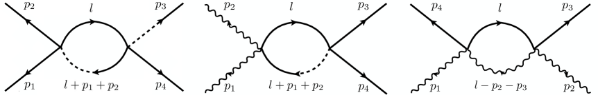
Figure 12: The Feynman diagrams for the one-loop renormalization of $\lambda$. The first diagram corrects $\langle\varphi(p_{1})\varphi(p_{2})\varphi(p_{3})\varphi(p_{4})\rangle$, while the other two would arise for $\langle\chi_{j}(p_{1})\chi_{j}(p_{2})\varphi(p_{3})\varphi(p_{4})\rangle$.

Note that while the finite piece of $I_{\omega\varphi^{3}}$ has nontrivial dependence of the external momenta, the pole is $p$-independent so we can cancel it against the tree level contribution in (G.5). This determines

$$Z_{\lambda}=1+\frac{3\lambda H}{(4\pi)^{3}\varepsilon},$$ (G.8)

the same result as in the previous section. Hence we get the same beta function (F.24).

Alternatively we could consider $\langle\chi_{j}(p_{1})\chi_{j}(p_{2})\varphi(p_{3})\varphi(p_{4})\rangle$. At one loop we have the two diagrams in Figure 12. Here too, at one-loop the dependence on the external momenta and $i,j$ indices is proportional to that in tree level, but now involving the other vertex $\chi_{i}^{2}\varphi^{2}$. The amputated function once again gives the same correction $z^{(1,1)}_{\lambda}$. This can be seen as a consequence of the equivalence of (2.21) with the SUSY theory (2.27). We omit the details.

Wavefunction renormalization

Here we will calculate the wavefunction renormalization constants $Z_{\varphi},Z_{\omega},Z_{\chi}$, which get the first correction at two loops (we will need it in our two-loop anomalous dimension computations). These renormalization constants are determined by requiring the 2-point functions $\langle\varphi(p)\omega(-p)\rangle$, $\langle\varphi(p)\varphi(-p)\rangle$ and $\langle\chi_{i}(p)\chi_{j}(-p)\rangle$ be free of $\varepsilon$ poles. These 2-point functions receive two-loop corrections shown in Figures 13 and 14.

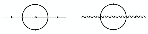
Figure 13: Two-loop corrections to $\langle\varphi(p)\omega(-p)\rangle$ and $\langle\chi_{i}(p)\chi_{j}(-p)\rangle$ (labels $i,j$ omitted).

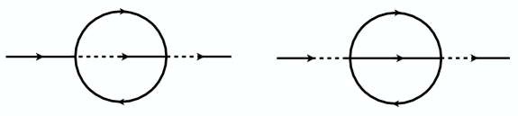
Figure 14: Two-loop corrections to $\langle\varphi(p)\varphi(-p)\rangle$.

These loop integrals are similar to the usual Wilson-Fisher two-loop field renormalization integral [106]. One integral common to all corrections is:

$$I_{\varphi\omega}(p^{2})=\frac{\lambda^{2}H^{2}}{(2\pi)^{2d}}\int\int\frac{d^{d}l_{1}d^{d}l_{2}}{(l_{1}^{2})^{2}(l_{2}^{2})^{2}(p+l_{1}+l_{2})^{2}}=\;-\frac{\lambda^{2}H^{2}p^{2}}{6(4\pi)^{6}\varepsilon}+O\left(\varepsilon^{0}\right).$$ (G.9)

For the correction to $\langle\varphi(p)\varphi(-p)\rangle$ we have an extra integral:

$$I_{\varphi\varphi}=\frac{\lambda^{2}H^{2}}{(2\pi)^{2d}}\int\int\frac{d^{d}l_{1}d^{d}l_{2}}{(l_{1}^{2})^{2}(l_{2}^{2})^{2}((p+l_{1}+l_{2})^{2})^{2}}=\;-\frac{\lambda^{2}H^{2}}{2(4\pi)^{6}\varepsilon}+O\left(\varepsilon^{0}\right).$$ (G.10)

Putting in the appropriate symmetry factors, we obtain the following two-loop corrected 2-point functions (where we keep $Z_{\varphi},Z_{\omega},Z_{\chi}$ at tree level but set them to one in the correction):

$$\left\langle\varphi(p)\omega(-p)\right\rangle = \frac{1}{p^{2}}\left[\frac{1}{Z_{\varphi}Z_{\omega}}-\frac{\lambda^{2}H^{2}}{12(4\pi)^{6}\varepsilon}+O\left(\lambda^{2}\varepsilon^{0}\right)\right],$$

$$\langle\chi_{i}(p)\chi_{j}(-p)\rangle = \frac{1}{p^{2}}\left[\frac{1}{Z_{\chi}^{2}}-\frac{\lambda^{2}H^{2}}{12(4\pi)^{6}\varepsilon}+O\left(\lambda^{2}\varepsilon^{0}\right)\right],$$ (G.11)

$$\langle\varphi(p)\varphi(-p)\rangle = \frac{H}{(p^{2})^{2}}\left[\frac{1}{Z_{\varphi}^{2}}-\frac{\lambda^{2}H^{2}}{12(4\pi)^{6}\varepsilon}+O\left(\lambda^{2}\varepsilon^{0}\right)\right].$$

Requiring that $\varepsilon$ poles cancel determines:

$$\hskip 23.99997ptZ_{\varphi}Z_{\omega}=Z_{\varphi}^{2}=Z_{\chi}^{2}=\>1-\frac{\lambda^{2}H^{2}}{12(4\pi)^{6}\varepsilon}\>+O(\lambda^{3}).$$ (G.12)

Thus we find $Z_{\varphi}=Z_{\omega}=Z_{\chi}$. In particular $Z_{\varphi}=Z_{\omega}$ can be interpreted as the non-renormalization of $H$. Recall that our theory is equivalent to the supersymmetric theory (2.27), and $H$ is a parameter in the SUSY transformations. As commented in section 3.1, dimensional regularization preserves full SUSY and hence $H$. (In section 7.1 we instead discussed that in other regularization schemes $H$ can renormalize, using a slightly different notation for wavefunction renormalization constants, see Eq. (7.2).)

Finally, from $Z_{\varphi},Z_{\omega},Z_{\chi}$ by the usual definitions we compute the anomalous dimensions of the fields:

$$\gamma_{\varphi}=\gamma_{\omega}=\gamma_{\chi}=\left[\frac{\partial\log Z_{\varphi}}{\partial\log\mu}\right]_{\lambda=\lambda_{\ast}}=\frac{\varepsilon^{2}}{108}+O\left(\varepsilon^{3}\right),$$ (G.13)

equal to $\gamma_{\widehat{\phi}}$ at the usual Wilson-Fisher fixed point, consistently with the dimensional reduction.

Appendix H Details of anomalous dimension computations

In this appendix we will show the details of the anomalous dimension computations presented in section 9. Throughout this section we will denote by $\gamma_{\mathcal{O}}=\Delta_{\mathcal{O}}-\Delta^{0}_{\mathcal{O}}$ the anomalous dimension for an operator $\mathcal{O}$, where $\Delta_{\mathcal{O}}$ is the dimension of $\mathcal{O}$ at the fixed point (3.7) and $\Delta_{\mathcal{O}}^{0}$ is its dimension at the Gaussian (free theory) fixed point at $d=6-\varepsilon$.

Recall that the three operator classes have the block-diagonal mixing structure shown in (F.11), which allows to compute anomalous dimensions in each class separately (although the true scaling susy-writable operators will have an admixture of susy-nulls, while non-susy-writables will have an admixture of both susy-writables and susy-nulls). We will try to remind the reader of that whenever a confusion might arise.

Susy-writable operators

As explained in section 8.3, susy-writable operators have well-defined anomalous dimensions equal to the ones of the Wilson-Fisher (WF) in $d=4-\varepsilon$ dimensions. Here we give a few examples of such operators and their anomalous dimensions. In this section we work at one loop and the reported computations have been performed using the OPE formalism from App. F.

In our computations we used the $\chi$-formulation, but in the discussions and in the comparison with WF it is also convenient to use the superfields. The superfield formulation by construction misses all contributions proportional to susy-null operators, which are instead non-vanishing in the $\chi$-formulation. As already mentioned several times, susy-null operators cannot generate susy-writables under RG (while the opposite may happen), so that their mixing matrix is triangular, which ensures that anomalous dimensions of susy-writable operators can be computed by setting to zero susy-null contributions. In the following we will use this shortcut. We will be also able to recover the susy-null contributions by asking that the complete operator is an eigenperturbation.

Let us start by considering the operators $(\Phi^{2})_{\theta\bar{\theta}},$ $\mathcal{T}^{\mu\mu}_{\theta\bar{\theta}}$, $\partial^{2}(\Phi^{2})_{\theta\bar{\theta}}$, $(\Phi^{4})_{\theta\bar{\theta}}$, $(\Phi^{2}\mathcal{T}^{\mu\mu})_{\theta\bar{\theta}}$ discussed in the main text. As a first step we rewrite all terms involving $\psi$, $\bar{\psi}$ using the $\chi$-formulation (see appendix C). It is then easy to check that the anomalous dimensions of these operators are respectively equal to $\varepsilon/3$, $0$, $\varepsilon/3$, $2\varepsilon$, $(13/9)\varepsilon$, as expected from the WF counterpart [39].

We can further study if some susy-null contributions should be added. It is easy to check that the first four operators above do not get modified by susy-null terms. On the other hand the last operator is an eigenpertubation only when we add to it a term proportional to $(\chi^{2})^{2}$, namely

$$(\Phi^{2}\mathcal{T}^{\mu\mu})_{\theta\bar{\theta}}+\frac{15}{26}(\chi^{2})^{2}.$$ (H.1)

As we explain in the main text, the only susy-writable operator which may play an important role in destabilizing the susy RG is the so called box superfield $B^{ab,cd}$, which transforms in the $(2,2)$ representation of $\operatorname{OSp}(d|2)$ (recall that unitarity bounds for this representation are too weak to ensure that the operator is irrelevant). Its WF counterpart is defined in the main text as

$$\widehat{B}_{\mu\nu{,}\rho\sigma}=\left(\widehat{\phi}_{,\mu\nu}\widehat{\phi}_{,\rho\sigma}\widehat{\phi}^{2}-\frac{2\widehat{d}}{\widehat{d}-2}\widehat{\phi}_{,\mu}\widehat{\phi}_{,\nu}\widehat{\phi}_{,\rho\sigma}\widehat{\phi}\right)^{Y}.$$ (H.2)

The anomalous dimension of (H.2) was computed in [39] and it equals $(7/9)\varepsilon$. We would like to reproduce this result by studying the superfield $\mathcal{B}^{ab,cd}$. This is a very non-trivial check that dimensional reduction works also for operators in non-trivial $\operatorname{OSp}(d|2)$ representations. While doing so, we will also show the explicit expression in components for this operator.

We mainly focus on $(\mathcal{B}^{\theta\bar{\theta},\theta\bar{\theta}})_{\theta\bar{\theta}}$, since this component is bosonic, supertranslation invariant (it is the highest component of a superfield) and it is a scalar with respect to $\operatorname{SO}(d)$. Because of these features, this operator is generated in our RG flow and could destabilize it (if it becomes relevant).

First let us spell out the $\operatorname{SO}(\widehat{d})$ Young symmetrizer denoted by $Y$ in (H.2). This is a tensor with two sets of four indices, each set transforming in the  $\operatorname{SO}(\widehat{d})$ representation $(2,2)$. By contracting the indices $\mu\nu\rho\sigma$ inside the brackets of (H.2) with one set, we obtain an operator depending on the second set of indices, which transforms properly in the $(2,2)$ irrep. It is convenient to represent the symmetrizer (see [107, 108, 109]) by contracting its eight indices with auxiliary $\mathbb{R}^{\widehat{d}}$ vectors— the symmetric indices in each row are contracted with the same vector. The first set is contracted with $X_{1}$ and $X_{2}$, while the second set with $Z_{1}$ and $Z_{2}.$ The result is expressed in the following polynomial form:

$$\!\!\!\!\Pi_{2,2}(X_{1},X_{2};Z_{1},Z_{2})=c_{2,2}\bigl{\{}-(X_{1}\cdot X_{1})(Z_{1}\cdot Z_{1})(X_{2}\cdot Z_{2})^{2}-2(X_{1}\cdot X_{2})^{2}(Z_{1}\cdot Z_{2})^{2}$$

$$+2(X_{1}\cdot X_{1})(Z_{1}\cdot Z_{2})(X_{2}\cdot Z_{1})(X_{2}\cdot Z_{2})+2(X_{1}\cdot X_{1})(X_{2}\cdot X_{2})(Z_{1}\cdot Z_{2})^{2}$$

$$+2(X_{1}\cdot X_{2})^{2}(Z_{1}\cdot Z_{1})(Z_{2}\cdot Z_{2})-2(X_{1}\cdot X_{1})(X_{2}\cdot X_{2})(Z_{1}\cdot Z_{1})(Z_{2}\cdot Z_{2})$$

$$+(\widehat{d}-1)(X_{2}\cdot X_{2})(Z_{1}\cdot Z_{1})(X_{1}\cdot Z_{2})^{2}-2(\widehat{d}-1)(X_{1}\cdot X_{2})(Z_{1}\cdot Z_{1})(X_{1}\cdot Z_{2})(X_{2}\cdot Z_{2})$$

$$-2(\widehat{d}-1)(X_{2}\cdot X_{2})(Z_{1}\cdot Z_{2})(X_{1}\cdot Z_{1})(X_{1}\cdot Z_{2})+2(\widehat{d}-1)(X_{1}\cdot X_{2})(Z_{1}\cdot Z_{2})(X_{1}\cdot Z_{2})(X_{2}\cdot Z_{1})$$

$$+2(\widehat{d}-1)(X_{1}\cdot X_{2})(Z_{1}\cdot Z_{2})(X_{1}\cdot Z_{1})(X_{2}\cdot Z_{2})+(\widehat{d}-1)(X_{2}\cdot X_{2})(Z_{2}\cdot Z_{2})(X_{1}\cdot Z_{1})^{2}$$ (H.3)

$$-2(\widehat{d}-1)(X_{1}\cdot X_{2})(Z_{2}\cdot Z_{2})(X_{1}\cdot Z_{1})(X_{2}\cdot Z_{1})+(\widehat{d}-1)(X_{1}\cdot X_{1})(Z_{2}\cdot Z_{2})(X_{2}\cdot Z_{1})^{2}$$

$$-(\widehat{d}-2)(\widehat{d}-1)(X_{1}\cdot Z_{2})^{2}(X_{2}\cdot Z_{1})^{2}+2(\widehat{d}-2)(\widehat{d}-1)(X_{1}\cdot Z_{1})(X_{1}\cdot Z_{2})(X_{2}\cdot Z_{1})(X_{2}\cdot Z_{2})$$

$$-(\widehat{d}-2)(\widehat{d}-1)(X_{1}\cdot Z_{1})^{2}(X_{2}\cdot Z_{2})^{2}+\widehat{d}(X_{1}\cdot X_{1})(Z_{1}\cdot Z_{1})(X_{2}\cdot Z_{2})^{2}$$

$$-2\widehat{d}(X_{1}\cdot X_{1})(Z_{1}\cdot Z_{2})(X_{2}\cdot Z_{1})(X_{2}\cdot Z_{2})\bigr{\}},$$

where $c_{2,2}=-\frac{1}{3(-2+\widehat{d})(-1+\widehat{d})}$ is a normalization constant which ensures that the symmetrizer is idempotent. In order to get back the indices it is then sufficient to take derivatives with respect to the auxiliary vectors. As explained in [1], this contracted form of the Young symmetrizer is also convenient since it trivially generalizes to $\operatorname{OSp}(d|2)\operatorname{representations}$, by considering vectors $X_{i},Z_{i}$ in $\mathbb{R}^{d|2}$ and the scalar product $X\cdot Y=X^{a}g_{{}_{ab}}Y^{b}$, with the usual $\operatorname{OSp}(d|2)$ metric $g_{ab}$. We stress that the dependence of the symmetrizer on the parameter $\widehat{d}$ must not be changed (indeed $\widehat{d}=d-2$ is equal to the supertrace).

By some manipulations of this projector, we are able to obtain the final form for the box superfield,

$$(\mathcal{B}^{\theta\bar{\theta},\theta\bar{\theta}})_{\theta\bar{\theta}}= \frac{1}{6}\bigl{\{}-\varphi^{2}\psi_{,\mu\nu}\bar{\psi}_{,\mu\nu}+\psi\bar{\psi}(-\varphi_{,\mu\nu}^{2}-20\varphi_{,\mu}\omega_{,\mu}+54\omega^{2})+4\varphi\varphi_{,\mu}(\psi_{,\nu}\bar{\psi}_{,\mu\nu}+\psi_{,\mu\nu}\bar{\psi}_{,\nu})$$ (H.5)

$$+2\varphi_{,\mu}\varphi_{,\nu}(\psi\bar{\psi}_{,\mu\nu}+\psi_{,\mu\nu}\bar{\psi})-2\varphi\varphi_{,\mu\nu}(\psi\bar{\psi}_{,\mu\nu}+\psi_{,\mu\nu}\bar{\psi})-42\varphi\omega\psi_{,\mu}\bar{\psi}_{,\mu}$$

$$+2\varphi\varphi_{,\mu\nu}(\psi_{,\mu}\bar{\psi}_{,\nu}+\psi_{,\nu}\bar{\psi}_{,\mu})+4\varphi_{,\mu}\varphi_{,\mu\nu}(\psi\bar{\psi}_{,\nu}+\psi_{,\nu}\bar{\psi})-\varphi\omega\varphi_{,\mu\nu}^{2}+54\varphi\omega^{3}$$

$$-12\omega\varphi_{,\mu}(\psi\bar{\psi}_{,\mu}+\psi_{,\mu}\bar{\psi})+10\varphi\omega_{,\mu}(\psi\bar{\psi}_{,\mu}+\psi_{,\mu}\bar{\psi})-30\psi\bar{\psi}\psi_{,\mu}\bar{\psi}_{,\mu}$$

$$+2\omega\varphi_{,\mu}\varphi_{,\nu}\varphi_{,\mu\nu}+4\varphi\omega_{,\mu}\varphi_{,\nu}\varphi_{,\mu\nu}+\varphi(2\varphi_{,\mu}\varphi_{,\nu}-\varphi\varphi_{,\mu\nu})\omega_{,\mu\nu}+5\varphi^{2}\omega_{,\mu}^{2}$$

$$-6\omega^{2}\varphi_{,\mu}^{2}-32\varphi\omega\varphi_{,\mu}\omega_{,\mu}\bigr{\}},$$

where for short the expression is written for $d=\widehat{d}+2=6$. We checked that this operator, upon substitution $\psi,\bar{\psi}\rightarrow\chi$ has indeed anomalous dimension $(7/9)\varepsilon$ as expected.

Notice that (H.5) contains the term $\psi\bar{\psi}\psi_{,\mu}\bar{\psi}_{,\mu}$ which can be mapped in two different ways (as explained in App. C, Eq. (C.7)) in terms of $\chi$. Both choices are equally good, since their difference is proportional to the susy-null operator $\partial^{2}(\chi^{2})^{2}$ (which can be set to zero for anomalous dimensions computations). As usual we can also determine the susy-null contribution by requiring that the full operator is an eigenperturbation: this gives the above $(\mathcal{B}^{\theta\bar{\theta},\theta\bar{\theta}})_{\theta\bar{\theta}}$ with $\psi\bar{\psi}\psi_{,\mu}\bar{\psi}_{,\mu}\rightarrow\frac{1}{4}\chi_{i}\chi_{i}\chi_{j,\mu}\chi_{j,\mu}+\frac{5}{84}\partial^{2}(\chi^{2})^{2}$.

As a final example we compute the anomalous dimensions of all susy-writable (and one susy-null) operators at dimensions $\Delta=10$ made of four fields. One of such operators is (H.5), and we would like to check that all of the others also have dimensions consistent from dimensional reduction. In practice we consider a list of 32 monomials: the 22 summands of (H.5) (terms of the form e.g. $\psi\bar{\psi}_{,\nu}+\psi_{,\nu}\bar{\psi}$ are counted as one after the $\psi,\bar{\psi}\rightarrow\chi$ map), the susy-null operator $\partial^{2}(\chi^{2})^{2}$ discussed above and the following 9 extra operators

$$\varphi_{,\mu}^{2}\chi_{,\nu}^{2},\quad\varphi_{,\mu}\chi_{,\mu}\varphi_{,\nu}\chi_{,\nu},\quad\varphi^{2}\varphi_{,\mu\nu\sigma}^{2},\quad\varphi\varphi_{,\mu}\varphi_{,\nu\sigma}\varphi_{,\mu\nu\sigma},\quad\varphi_{,\nu}^{2}\varphi_{,\mu\sigma}^{2}$$ (H.6)

$$\varphi\varphi_{,\mu\nu}\varphi_{,\mu\sigma}\varphi_{,\nu\sigma},\quad\varphi_{,\mu}\omega_{,\mu}\varphi_{,\nu}^{2},\quad\varphi_{,\mu}\varphi_{,\nu}\varphi_{,\sigma}\varphi_{,\mu\nu\sigma},\quad\varphi_{,\nu}\varphi_{,\sigma}\varphi_{,\mu\nu}\varphi_{,\mu\sigma}.$$

This list of 32 monomials is closed upon renormalization, mixing in a non-trivial way. Diagonalizing the resulting $32\times 32$ mixing matrix gives the following list of anomalous dimensions:

$$2\varepsilon,2\varepsilon,\frac{13\varepsilon}{9},\frac{13\varepsilon}{9},\frac{13\varepsilon}{9},\frac{13\varepsilon}{9},\frac{13\varepsilon}{9},\frac{19\varepsilon}{15},\frac{10\varepsilon}{9},\frac{10\varepsilon}{9},\varepsilon,\varepsilon,\varepsilon,\varepsilon,$$ (H.7)

$$\frac{14\varepsilon}{15},\frac{8\varepsilon}{9},\frac{8\varepsilon}{9},\frac{8\varepsilon}{9},\frac{8\varepsilon}{9},\frac{7\varepsilon}{9},\frac{7\varepsilon}{9},\frac{7\varepsilon}{9},\frac{7\varepsilon}{9},\frac{\varepsilon}{2},\frac{\varepsilon}{2},\frac{4\varepsilon}{9},\frac{\varepsilon}{3},\frac{2\varepsilon}{9},\frac{\varepsilon}{9},0,0,0.$$

Let us see next how this list can be related to WF computations. First, we would like to emphasize that many of the numbers in (H.7) are associated to descendants. Indeed, we can redo the computation only using equivalence classes of operators defined up to total derivatives (as discussed in appendix F). The result is that only 8 of the above operators are not descendants. The associated anomalous dimensions are $\frac{10\varepsilon}{9},\frac{14\varepsilon}{15},\frac{8\varepsilon}{9},\frac{7\varepsilon}{9},\frac{\varepsilon}{2},\frac{\varepsilon}{3},\frac{\varepsilon}{9},0,0$. This also explains why in (H.7) there are many repeated anomalous dimensions: they correspond to total derivatives of different components of the superfield. To clarify this, let us focus on the anomalous dimension $\frac{7\varepsilon}{9}$ (the one of the box operator). This appears four times in (H.7) and only one of these is not a total derivative —this indeed corresponds to the operator (H.5). The other three occurrences are related to the following descendants (we also checked this explicitly):

$$\partial^{2}(\mathcal{B}^{\theta\bar{\theta},\theta\bar{\theta}})_{0},\quad\partial_{\mu}\partial_{\nu}(\mathcal{B}^{\theta\bar{\theta},\mu\nu})_{0},\quad\partial_{\mu}(\mathcal{B}^{\theta\bar{\theta},\theta\mu})_{\bar{\theta}}.$$ (H.8)

E.g. the first one, before applying $\partial^{2}$, takes the form

$$(\mathcal{B}^{\theta\bar{\theta},\theta\bar{\theta}})_{0} \rightarrow -\frac{1}{6}\varphi^{2}\varphi_{,\mu\nu}^{2}+\frac{2}{3}\varphi\varphi_{,\mu}\varphi_{,\nu}\varphi_{,\mu\nu}-\frac{5}{6}\varphi^{2}\chi_{i,\mu}^{2}+\frac{10}{3}\varphi\chi_{i}\varphi_{\mu}\chi_{i,\mu}-2\varphi\omega\varphi_{,\mu}^{2}$$ (H.9)

$$+\frac{7\varphi^{2}\omega^{2}}{3}-\frac{20}{3}\varphi\chi_{i}^{2}\omega-\left[\frac{10(\chi_{i}^{2})^{2}}{7}\right],$$

where we also included, in square brackets, the susy-null contribution.

We also notice that different anomalous dimensions in (H.7) occur a different number of times. It is easy to see why this happens. This depends on the superprimary $\operatorname{Osp}(d|2)$ representation, and on how many times we need to differentiate to get to the needed dimension. E.g. $2\varepsilon$ in (H.7) is related to the superprimary  $\Phi^{4}$ in the following two combinations: $(\partial^{2})^{2}\Phi_{\theta\bar{\theta}}^{4}$, $(\partial^{2})^{3}\Phi_{0}^{4}$. Here, since $\Phi^{4}$ is a scalar, there is a single $\operatorname{OSp}$ component to use (in constrast with non-scalar operators). Also only total derivatives appear because the superfield itself has too low bare dimension: $[\Phi_{0}^{4}]=4$, $[\Phi_{\theta\bar{\theta}}^{4}]=6$. As a final example, the value $\frac{13\varepsilon}{9}$ in (H.7) is related to five possible descendants of the superfield $\Phi^{2}\mathcal{T}^{ab}$: $(\partial^{2})^{2}(\Phi^{2}\mathcal{T}^{\theta\bar{\theta}})_{0}$, $\partial^{2}\partial_{\mu}\partial_{\nu}(\Phi^{2}\mathcal{T}^{\mu\nu})_{0}$, $\partial^{2}\partial_{\mu}(\Phi^{2}\mathcal{T}^{\mu\bar{\theta}})_{\theta}$, $\partial^{2}(\Phi^{2}\mathcal{T}^{\theta\bar{\theta}})_{\theta\bar{\theta}}$, $\partial_{\mu}\partial_{\nu}(\Phi^{2}\mathcal{T}^{\mu\nu})_{\theta\bar{\theta}}$.

We do not present here a detailed explanation for all anomalous dimensions in (H.7). However we stress that we checked that they are all in agreement with available WF results: not only the anomalous dimensions match but also the occurrences (of primaries and descendants) are the ones expected.

Most of the checks are done by comparing with table 4 of [39] (using the entries with $n=4$ fields), where all operators built out of $5$ or less derivatives are presented. However the list (H.7) is also sensitive to operators with six derivatives: indeed the lowest component of a superfield with four $\Phi$’s and six derivatives has dimension $10$. Unfortunately such operators were not fully classified in the WF literature, except for a scalar operator considered in [34] with $\gamma=\varepsilon/3$ (see equation (3.12)), which indeed matches our computation.

We can therefore predict that in the WF spectrum of operators with four fields and six derivatives, there are three operators with anomalous dimensions $0$, $\varepsilon/9$, $(14/15)\varepsilon$. We can further say something about their possible $\operatorname{SO}(\widehat{d})$ representation. Indeed the operators in our list must have an even number of indices which are set to $\theta$ and $\bar{\theta}$ (otherwise the resulting operator would be fermionic or it would not be an $\operatorname{SO}(\widehat{d})$ scalar). We thus conclude that these three operators must transform either in the scalar, or spin two, or $(2,2)$ representation of $\operatorname{SO}(\widehat{d})$.

Finally let us comment on the three operators with $\gamma=0$. Only one of them is a descendant: the susy-null operator $\partial^{2}(\chi^{2})^{2}$. One of the other two operators is a primary, an operator with six derivatives. The third operator in this group is actually not an eigenvector, but a generalized eigenvector forming a logarithmic multiplet together with the $\gamma=0$ primary. This is a recurrent feature of our non-unitary theory: mixing matrices may not be fully diagonalizable and can be organized in Jordan blocks, as discussed around Eq. (F.6).

Susy-null leaders

We next consider all the susy-null leaders with 6d classical dimension up to 12 (one at dimension 8, one at 10, and four at 12). For each of them we compute the one-loop anomalous dimension, or the two-loop one if the one-loop result is trivial. We use the OPE method at one loop, and Feynman diagrams whenever we have to go to two loops.

$\Delta^{0}=8+O(\varepsilon)$, $n=4$

The lowest susy-null leader is $(\chi_{i}^{2})^{2}$, of classical dimension $\Delta^{0}=8-2\varepsilon$ in $d=6-\varepsilon$ (see Table 1). It is easy to see that it does not receive any anomalous dimension at one loop, so we proceed to study the 2-loop contribution. Denoting by $((\chi_{i}^{2})^{2})^{B}$ the operator built of bare fields, and by $(\chi_{i}^{2})^{2}$ the renormalized operator whose correlators should be free of poles in $\varepsilon$, they are related by

$$((\chi_{i}^{2})^{2})^{B}=Z\,(\chi_{i}^{2})^{2},$$ (H.10)

To find the renormalization factor $Z$ we consider the correlator $\langle(\chi_{i}^{2})^{2}(p=0)\chi_{j}(p_{1})\chi_{k}(p_{2})\chi_{l}(p_{3})\chi_{m}(p_{4})\rangle$. A nonzero two-loop diagram is shown in Figure 4. Another two loop diagram (a double bubble diagram of the type shown in Figure 15) vanishes because it is proportional to $n$, from contractions of the $K_{ij}$ matrices in the $\chi$-$\chi$ propagator (E.2). At two loops we must also consider the propagator computed in section G.2.

Taking everything into account, the two-loop corrected amputated correlator equals the tree-level one, times

$$Z_{\,}^{-1}+\left[I_{(\chi_{i}^{2})^{2}}+\left(\text{t,u}\operatorname{channels}\right)\right]+\frac{1}{4}\sum_{i=1}^{4}I_{\varphi\omega}(p_{i}^{2})/p_{i}^{2}.$$ (H.11)

Here $I_{\varphi\omega}$ is the integral in (G.9) which comes from the external leg corrections. The $I_{(\chi_{i}^{2})^{2}}$ comes from the loop diagram of Figure 4. It is given by (see [106] for the standard details):

$$I_{(\chi_{i}^{2})^{2}}=\frac{H^{2}\lambda^{2}}{(2\pi)^{2d}}\int\frac{d^{d}l_{1}d^{d}l_{2}}{l_{1}^{2}(l_{2}^{2})^{2}(l_{1}+p_{3}+p_{4})^{2}((l_{1}+l_{2}-p_{1})^{2})^{2}}=\frac{H^{2}\lambda^{2}}{2(4\pi)^{6}\varepsilon}+O\left(\varepsilon^{0}\right).$$ (H.12)

The $Z_{\,}$ is obtained by demanding that $\varepsilon^{-1}$ poles cancel:

$$Z_{\,}^{-1}=1-\frac{4}{3}\frac{H^{2}\lambda^{2}}{(4\pi)^{6}\varepsilon}.$$ (H.13)

From this we get the anomalous dimension of $(\chi_{i}^{2})^{2}$ as follows:

$$\gamma_{(\chi_{i}^{2})^{2}}=\mu\frac{\partial}{\partial\mu}\log Z=-\frac{8}{27}\varepsilon^{2}.$$ (H.14)

$\Delta^{0}=10+O(\varepsilon)$, $n=6$

The next susy-null leader is $\varphi^{2}(\chi_{i}^{2})^{2}$ (Table 7), of bare dimension $\Delta^{0}=10-3\varepsilon$. It gets a nonzero one-loop anomalous dimension, which we compute by the OPE method (App. F). The following OPEs are important:

$$\varphi^{2}(\chi_{i}^{2})^{2}(x)\times\chi_{j}^{2}\varphi^{2}(0) \sim 32\langle\varphi(x)\varphi(0)\rangle_{0}\langle\chi_{i}(x)\chi_{j}(0)\rangle_{0}\,\varphi^{2}(\chi_{k}^{2})\chi_{i}\chi_{j}(0)+\ldots$$

$$\varphi^{2}(\chi_{i}^{2})^{2}(x)\times\omega\varphi^{3}(0) \sim 6\langle\varphi(x)\varphi(0)\rangle_{0}\langle\varphi(x)\omega(0)\rangle_{0}\,\varphi^{2}(\chi_{i}^{2})^{2}(0)+\ldots$$ (H.15)

From this and using the formula (F.18) we get

$$\gamma_{\varphi^{2}(\chi_{i}^{2})^{2}}=\left[\frac{9H\lambda}{64\pi^{3}}\right]_{\lambda=\lambda_{\ast}}=3\varepsilon+O\left(\varepsilon^{2}\right).$$ (H.16)

$\Delta^{0}=12+O(\varepsilon)$, $n=6$

At dimension $\Delta^{0}=12-3\varepsilon$ we have three independent susy-null leaders which are composites of 6 fields. Two of them are shown in Table 7 and the third in Eq. (D.11).

To compute their anomalous dimensions it is convenient to work with equivalence classes of operators defined up to total derivatives (as discussed in the end of appendix F.1). We can parametrize the equivalence classes by the following three operators: $\mathcal{O}_{1}=\varphi\omega(\chi^{2})^{2},\>\mathcal{O}_{2}=(\chi^{2})^{3}$ and $\mathcal{O}_{3}=\frac{1}{H}\left(\partial\varphi\right)^{2}(\chi_{i}^{2})^{2}$. E.g. $\varphi\partial\varphi(\chi_{i}\partial\chi_{i})(\chi_{j}^{2})$ is not considered as an independent operator since it can be written in terms of $\mathcal{O}_{1}$ and $\mathcal{O}_{2}$ up to a total derivative, namely $\varphi\partial\varphi(\chi_{i}\partial\chi_{i})(\chi_{j}^{2})=\frac{1}{4}\partial^{\mu}\left[\varphi\partial_{\mu}\varphi(\chi_{j}^{2})^{2}\right]+\frac{H}{4}\mathcal{O}_{1}-\frac{H}{4}\mathcal{O}_{2}$.

To compute the mixing matrix we consider the following OPEs of the operators $\mathcal{O}_{i}$ with the interaction $\mathcal{V}$

$$\varphi\omega(\chi^{2})^{2}(0)\times\chi^{2}\varphi^{2}(x) \sim 16\langle\varphi\varphi\rangle_{0}\langle\chi_{i}\chi_{j}\rangle_{0}\>\varphi\omega\chi^{2}\chi_{i}\chi_{j}+2\langle\varphi\varphi\rangle_{0}\langle\varphi\omega\rangle_{0}(\chi^{2})^{3}$$

$$+8x^{\mu}x^{\nu}\langle\varphi\omega\rangle_{0}\langle\chi_{i}\chi_{j}\rangle_{0}\>\varphi\chi^{2}\chi_{i}\partial_{\mu}\partial_{\nu}\left(\varphi\chi_{j}\right)+\ldots$$

$$\varphi\omega(\chi^{2})^{2}(0)\times\varphi^{3}\omega(x) \sim 6\langle\varphi\varphi\rangle_{0}\langle\varphi\omega\rangle_{0}\varphi\omega(\chi^{2})^{2}+3x^{\mu}x^{\nu}\langle\varphi\omega\rangle_{0}\langle\varphi\omega\rangle_{0}\left(\partial_{\mu}\partial_{\nu}\varphi^{2}\right)(\chi^{2})^{2}+\ldots$$ (H.18)

$$(\chi^{2})^{3}(0)\times\chi^{2}\varphi^{2}(x) \sim 24\langle\chi_{i}\chi_{j}\rangle_{0}\langle\chi_{i}\chi_{j}\rangle_{0}\left(\partial_{\mu}\partial_{\nu}\varphi^{2}\right)(\chi^{2})^{2}$$ (H.19)

$$+6\langle\chi_{i}\chi_{j}\rangle_{0}\langle\chi_{i}\chi_{k}\rangle_{0}\left(\partial_{\mu}\partial_{\nu}\varphi^{2}\right)\chi^{2}\chi_{j}\chi_{k}+\ldots$$

$$\left(\partial\varphi\right)^{2}(\chi^{2})^{2}(0)\times\varphi^{3}\omega(x) \sim 6x^{\mu}x^{\nu}\partial^{\sigma}\langle\varphi\varphi\rangle_{0}\,\partial_{\sigma}\langle\varphi\omega\rangle_{0}\left(\partial_{\mu}\partial_{\nu}\varphi^{2}\right)(\chi^{2})^{2}$$ (H.20)

$$+6\partial^{\sigma}\langle\varphi\varphi\rangle_{0}\,\partial_{\sigma}\langle\varphi\varphi\rangle_{0}\varphi\omega(\chi^{2})^{2}+\ldots$$

$$\left(\partial\varphi\right)^{2}(\chi^{2})^{2}(0)\times\chi^{2}\varphi^{2}(x) \sim -32x^{\nu}\langle\chi_{i}\chi_{j}\rangle_{0}\partial^{\mu}\langle\varphi\varphi\rangle_{0}\left(\partial_{\mu}\varphi\right)\chi^{2}\chi_{i}\partial_{\nu}\left(\varphi\chi_{j}\right)$$ (H.21)

$$+2\partial\langle\varphi\varphi\rangle_{0}\partial\langle\varphi\varphi\rangle_{0}(\chi^{2})^{3}+\ldots$$

In the above OPEs we have expanded the r.h.s. in $x$ wherever needed and kept only the terms that give $1/\varepsilon$ pole. Following the discussion in appendix F.1, we finally obtain the $3\times 3$ anomalous dimension matrix:

$$\Gamma=\frac{\varepsilon}{18}\left(\begin{array}[]{ccc}24&-12&2\\ 3&0&3\\ -2&12&20\end{array}\right).$$ (H.22)

This matrix is not fully diagonalizable, but it admits a Jordan decomposition (see around formula (F.6)) with eigenvalues 0 and $(11/9)\varepsilon$, to which there correspond true eigenvectors $e^{(1)}=\left\{-1,-\frac{11}{6},1\right\}$ and $e^{(2)}=\{-1,0,1\}$. There is also a generalized eigenvector $e^{(3)}=\left\{-\frac{99}{2\varepsilon},-\frac{27}{4\varepsilon},0\right\}$ which forms a rank-2 Jordan block with $e^{(2)}$, namely $\left(\Gamma_{ij}-\frac{11}{9}\varepsilon\delta_{ij}\right)e_{j}^{(3)}=e_{i}^{(2)}$. Therefore, corresponding to the anomalous dimension $\frac{11}{9}\varepsilon$, there is a $2\times 2$ Jordan block and a logarithmic multiplet $\{\mathcal{O}_{1}^{R},\mathcal{O}_{2}^{R}\}$, such that

$$D\left(\begin{array}[]{c}\mathcal{O}_{2}^{R}\\ \mathcal{O}_{1}^{R}\end{array}\right)=\left(\begin{array}[]{cc}12-\frac{16\varepsilon}{9}&\varepsilon\\ 0&12-\frac{16\varepsilon}{9}\end{array}\right)\left(\begin{array}[]{c}\mathcal{O}_{2}^{R}\\ \mathcal{O}_{1}^{R}\end{array}\right),$$ (H.23)

where the dilatation operator $D$ is acting on the renormalized operators $\mathcal{O}_{1}^{R}\equiv-\mathcal{O}_{1}+\mathcal{O}_{3}$ and $\mathcal{O}_{2}^{R}\equiv-\frac{99}{2}\mathcal{O}_{1}-\frac{27}{4}\mathcal{O}_{2}$. Here the operators $\mathcal{O}_{1}^{R}$ and $\mathcal{O}_{2}^{R}$ should not be considered as the actual renormalized operators, since they only parametrize the equivalence classes of operators up to derivatives.

For the sake of completeness we also performed a much more general computation which gives us the exact form of the renormalized operators. Computing the anomalous dimensions matrix of the 49 possible operators which are built out of 6 fields and have dimensions 12 in $d=6,$ we obtained that $\mathcal{O}_{1}^{R}$ was actually a correct eigenperturbation. On the other hand, the operator $\mathcal{O}_{2}^{R}$ should have been corrected by some total derivatives, namely by adding to it $\frac{231}{32}\partial_{\mu}(\varphi_{,\mu}\varphi\chi_{i}^{2}\chi_{j}^{2})-\frac{33}{16}\partial_{\mu}(\varphi^{2}\chi_{i}\chi_{i,\mu}\chi_{j}^{2})$.

$\Delta^{0}=12+O(\varepsilon)$, $n=8$

With 8 fields and dimension $\Delta=12+O\left(\varepsilon\right)$ we have a single susy-null leader, $\varphi^{4}(\chi^{2})^{2}$ (See Table 8). Its $O\left(\varepsilon\right)$ anomalous dimension can be obtained from the following OPEs:

$$\varphi^{4}(\chi^{2})^{2}(0)\times\chi^{2}\varphi^{2}(x) \sim 64\langle\varphi\varphi\rangle_{0}\langle\chi_{i}\chi_{j}\rangle_{0}\>\varphi^{4}\chi^{2}\chi_{i}\chi_{j}$$

$$\varphi^{4}(\chi^{2})^{2}(0)\times\varphi^{3}\omega(x) \sim 36\langle\varphi\varphi\rangle_{0}\langle\varphi\omega\rangle_{0}\varphi^{4}(\chi^{2})^{2}.$$ (H.24)

Following (F.18) we get the anomalous dimension:

$$\gamma_{\varphi^{4}(\chi^{2})^{2}}=\frac{22\varepsilon}{3}.$$ (H.25)

Non-susy-writable leaders

We will now compute the anomalous dimensions for some specific non-susy writable leaders. For $\Delta\leqslant 12$ the only non-susy writable leader operator comes from the Feldman $\mathcal{F}_{6}$. We will consider this operator first and then will generalize to higher Feldman operators $\mathcal{F}_{k}$. This way we revisit the result of [30] that these operators have negative leading anomalous dimensions.

As shown in the main text the leader for Feldman operators have the structure:

$$(\mathcal{F}_{k})_{L} = \sum_{l=2}^{k-2}(-1)^{l}\binom{k}{l}\left(\sum\nolimits^{\prime}\chi^{l}_{i}\right)\left(\sum\nolimits^{\prime}\chi^{k-l}_{j}\right).$$ (H.26)

In particular $(\mathcal{F}_{6})_{L}=(\chi_{i}^{3})^{2}-\frac{3}{2}(\chi_{i}^{2})(\chi_{i}^{4})$ up to a constant factor. We will see in a second that $(\mathcal{F}_{6})_{L}$ has no anomalous dimension at one loop, so we are setting up a two-loop computation. Let $\mathcal{O}^{B}_{i}$ be all leader operators of bare dimension 12 with which $\mathcal{O}^{B}_{1}=(\mathcal{F}_{6})_{L}$ might mix, related to the renormalized operators by $\mathcal{O}^{B}_{i}=Z_{ij}\mathcal{O}_{j}$. Since $(\mathcal{F}_{6})_{L}$ is the lowest non-susy-writable leader, all these other operators are susy-null or susy-writable, hence the mixing matrix has the form (see (F.11))

$$Z=\left(\begin{array}[]{ccc}Z_{11}&\ast&\ldots\\ 0&\ast&\ldots\\ 0&\ast&\ldots\\ \vdots&\vdots&\ddots\end{array}\right),$$ (H.27)

i.e. in the first column only $Z_{11}$ is nonzero. Because of this, we only need to know $Z_{11}$ to compute the anomalous dimension of $(\mathcal{F}_{6})_{L}$. We would need to know the potentially nonzero entries marked by $\ast$ to compute the full eigenoperator, but we will not do this here.

To compute $Z_{11}$ we consider the correlator $\langle(\mathcal{F}_{6})_{L}(p=0)\chi_{i_{1}}(p_{1})\ldots\chi_{i_{6}}(p_{6})\rangle$. It is easy to see that there is no one-loop diagram which contributes to this correlator. This implies that $O(\lambda)$ correction to $Z_{11}$ vanishes, i.e. as promised $(\mathcal{F}_{6})_{L}$ has no one-loop anomalous dimension. [On the other hand some of the entries marked by $\ast$ in the first row are nonzero at one loop. As a result the eigenoperator gets a susy-null admixture already at one loop. See section H.3.1 for a discussion.] At two loops the correlator gets contributions from the two diagrams in Fig. 15 (for $k=6$), both with a $1/\varepsilon$ pole.

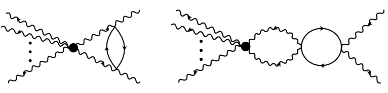
Figure 15: Two-loop diagrams correcting the correlator $\langle(\mathcal{F}_{k})_{L}(p=0)\chi_{i_{1}}(p_{1})\ldots\chi_{i_{k}}(p_{k})\rangle$.

The first diagram’s tensor structure in the $\chi_{i}$ indices is precisely that of $(\mathcal{F}_{6})_{L}$ itself (this is obvious because of $K^{2}=K$, see (E.4)). Performing $K_{ij}$-tensor contractions, the second diagram is instead proportional to the tree-level diagram with insertion of the susy-null operator $(\chi_{i}^{2})^{3}$. This is an example of a susy-null admixture, a nonzero $\ast$ entry in the first row of (H.27). So only the first diagram contributes to $Z_{11}$.

That the second diagram does not contribute to $Z_{11}$ in fact holds for general $k$, and we will need this fact below, so let us show it. Its tensor structure splits into two groups of indices separated by the $\varphi$ loop. The right tensor structure is just that of $\chi^{2}_{i}$. The left tensor structure with its $\chi$-loop can be obtained by applying $K_{rs}\frac{\delta}{\delta\chi_{r}}\frac{\delta}{\delta\chi_{s}}$ to the Feldman leader expression. This calculation is greatly simplified using the equivalent equation (see (5.16))

$$(\mathcal{F}_{k})_{L} = 2\sum_{i=2}^{n}(-\chi_{i})^{k}+\sum_{i,j=2}^{n}(\chi_{i}-\chi_{j})^{k},$$ (H.28)

and it gives $2k(k-1)(\mathcal{F}_{k-2})_{L}$ after a few lines of algebra, i.e. a multiple of the lower Feldman leader. Thus the total tensor structure is that of $(\chi^{2}_{i})(\mathcal{F}_{k-2})_{L}$. For $k=6$ this reduces to $(\chi_{i}^{2})^{3}$ as claimed, since $(\mathcal{F}_{4})_{L}\propto(\chi^{2}_{i})^{2}$.

Let us next evaluate the first diagram in (15), also for general $k$. The loop integral is the same as $I_{(\chi_{i}^{2})^{2}}$ in (H.12), the computation being similar to the one for the $(\chi^{2})^{2}$ in section H.2.1. (Eq. (H.29) below reduces to (H.13) for $k\rightarrow 4$.) Taking into account external leg corrections and combinatorial factors, we get:

$$\hskip 14.22636ptZ_{11}^{-1}=1-\frac{k(k-1)}{4}[I_{(\chi_{i}^{2})^{2}}]_{1/\varepsilon}-\frac{k}{4}\left[\frac{I_{\varphi\omega}(p^{2})}{p^{2}}\right]_{1/\varepsilon}=1-\frac{k(3k-4)}{24}\frac{H^{2}\lambda^{2}}{(4\pi)^{6}\varepsilon}.$$ (H.29)

Setting here $k=6$ we get the anomalous dimension:

$$\gamma_{(\mathcal{F}_{6})_{L}}=-\frac{7}{9}\varepsilon^{2}.$$ (H.30)

With a small extra input we can upgrade the above discussion and extract the anomalous dimensions of $(\mathcal{F}_{k})_{L}$ for general $k$. We just need to check if one more element of the mixing matrix is zero. We have seen above that $(\mathcal{F}_{k})_{L}$ requires adding $(\chi^{2}_{i})(\mathcal{F}_{k-2})_{L}$ to get a finite operator. For $k=6$ the latter operator was susy-null, hence the inverse mixing was guaranteed not to happen. For $k>6$ the operator $(\chi^{2}_{i})(\mathcal{F}_{k-2})_{L}$ is non-susy-writable, so we need to see if it mixes back to $(\mathcal{F}_{k})_{L}$. It is however easy to see that this does not happen. Using Eq. (H.26), operator $(\chi^{2}_{i})(\mathcal{F}_{k-2})_{L}$ can be expanded in monomials each of which is a product of three $O(n-2)$ singlets of the form $(\chi^{2}_{i_{1}})(\chi_{i_{2}}^{a})(\chi_{i_{3}}^{b})$, where $a+b=k-2$. If any of these singlets is plugged into the second diagram in Fig. 15, it returns a monomial which is a product of four or three singlets (depending on how the $\chi$-loop is contracted). Since $(\mathcal{F}_{k})_{L}$ is made of products of two singlets, its tensor structure cannot arise. This discussion implies that the anomalous dimension of $(\mathcal{F}_{k})_{L}$ for any $k$ is not modified by mixing with $(\chi^{2}_{i})(\mathcal{F}_{k-2})_{L}$ and can be computed from $Z_{11}$ given in (H.29). We obtain:

$$\gamma_{(\mathcal{F}_{k})_{L}}=-\frac{k(3k-4)}{108}\varepsilon^{2}.$$ (H.31)

This nicely matches the result of [30]. In the future it would be interesting to analyze other non-susy-writable leaders with the same classical dimension as $(\mathcal{F}_{k})_{L}$ for $k>6$, one obvious example being $\left(2\omega\varphi+\chi_{i}^{2}\right)(\mathcal{F}_{k-2})_{L}$, to see if any of these has the corrected dimension even lower than $(\mathcal{F}_{k})_{L}.$

Remark on admixture of susy-nulls

As mentioned above, the leader $(\mathcal{F}_{6})_{L}$ experiences a susy-null mixing already at one-loop level, which does not modify its anomalous dimension (zero at one loop), but does modify the form of the eigenvector. In fact the correct eigenvector at one loop is the linear combination:

$$(\chi_{i}^{3})^{2}-\frac{3}{2}(\chi_{i}^{2})(\chi_{j}^{4})+\frac{3}{2}(\chi_{i}^{2})^{3},$$ (H.32)

where the first two terms are (proportional to) $(\mathcal{F}_{6})_{L}$, while the last term is susy-null. The form of this one-loop eigenvector can be determined e.g. using the OPE method (App. F).

Here we would like to point out that (H.32) can also be determined using group theory reasoning. Namely, we expect that leaders with well-defined anomalous dimensions will transform in irreducible $O(n-2)$ representations, which should correspond to symmetric traceless tensors. Eq. (H.32) can be written as the contraction of 6 $\chi$’s with the symmetric $6$-tensor

$$T=\left(\delta_{3}\otimes\delta_{3}-\frac{3}{2}\delta_{2}\otimes\delta_{4}+\frac{3}{2}\delta_{2}\otimes\delta_{2}\otimes\delta_{2}\right)_{\operatorname{sym}}.$$ (H.33)

Here $\operatorname{sym}$ is the symmetrization, and $\delta_{p}$ denotes the rank $k$-tensor whose only nonzero components are $(\delta_{p})_{\underbrace{\scriptstyle ii\ldots i}_{p}}=1$ i.e. when all $p$ indices coincide (the indices run from 2 to $n$). E.g. $(\delta_{2})_{ij}=\delta_{ij}$ is the Kronecker delta tensor, while $\delta_{1}$ is the $(1,1,\ldots)$ vector. The appropriate trace taking into account the constraint $\sum\nolimits^{\prime}\chi_{i}=0$ is:

$$(\operatorname{tr}^{\prime}T)_{\ldots}=\sum_{i,j=2}^{n}(\delta_{ij}+\Pi_{ij})T_{ij\ldots}.$$ (H.34)

It is then easy to work out (we define $\delta_{0}=-1$, a constant):

$$\operatorname{tr}^{\prime}\delta_{p} = 2\delta_{p-2},$$ (H.35)

$$\operatorname{tr}^{\prime}(\delta_{p}\otimes\delta_{q})_{\operatorname{sym}} = [A_{p,q}2\delta_{p-2}\otimes\delta_{q}+A_{q,p}2\delta_{p}\otimes\delta_{q-2}+(1-A_{p,q}-A_{q,p})(\delta_{p+q-2}+\delta_{p-1}\otimes\delta_{q-1})]_{\operatorname{sym}},$$

where $A_{p,q}=\binom{p+q-2}{p-2}\left/\binom{p+q}{p}\right.=\frac{p(p-1)}{(p+q)(p+q-1)}$, and similarly for higher tensor products. Using these rules, one can check that the tensor (H.33) is indeed traceless, while it would not have been traceless without the last term.

Appendix I Remarks about tuning the disorder distribution

As discussed in section 11.2.1, one might be able to look for the SUSY fixed point in numerical simulations of the RFIM, by tuning the disorder distribution within a family depending on more than one parameter. Here we discuss some ideas about what parameter to tune, to set the relevant operator to 0, assuming for simplicity that a single perturbation has turned relevant, the one corresponding to the susy-null leader $(\chi^{2})^{2}$. This discussion is meant as schematic and non-rigorous.

Our starting point is the analysis of Brézin-De Dominicis ([28], Section 1) who used the Hubbard-Stratonovich identity to rewrite an Ising spin system in terms of a scalar field. Introducing replicas and integrating out the disorder, they arrived at the system of $n$ scalar fields on the lattice with the $S_{n}$-invariant potential ([28], Eq. (1.9))

$$V = \frac{1}{2}(\tau_{2}-1)\sigma_{2}-\frac{\tau_{2}}{2}\sigma_{1}^{2}+\frac{1}{12}(1+3\tau_{4}-4\tau_{2})\sigma_{4}+\frac{1}{24}(3\tau_{2}^{2}-\tau_{4})\sigma_{1}^{4}$$ (I.1)

$$+\frac{1}{8}(\tau_{2}^{2}-\tau_{4})\sigma_{2}^{2}+\frac{1}{3}(\tau_{2}-\tau_{4})\sigma_{1}\sigma_{3}-\frac{1}{4}(\tau_{2}^{2}-\tau_{4})\sigma_{1}^{2}\sigma_{2}+O(\phi^{6}),$$

where $\sigma_{k}=\sum_{i=1}^{n}\phi_{i}^{k}$  as in section 5.1, and the quantities $\tau_{p}$ are defined as

$$\tau_{p}=\int_{-\infty}^{\infty}dhP(h)(\cosh h)^{n}(\tanh h)^{p}\hskip 1.69998pt\rightarrow\int_{-\infty}^{\infty}dh\,P(h)(\tanh h)^{p}\qquad(n\rightarrow 0).$$ (I.2)

Now let us refer to the toy model RG analysis in App. B. We can express the quartic part of the potential in terms of eigenperturbations given in Table 4: $\mathcal{O}_{1}=\sigma_{4}$, $\mathcal{O}_{2}=\sigma_{1}^{4}$, $\mathcal{O}_{3}=\sigma_{1}\sigma_{2}^{2}$, $\mathcal{O}_{4}=\sigma_{2}^{2}+2\sigma_{1}\sigma_{3}$ and $\mathcal{O}_{5}=\sigma_{2}^{2}-\frac{4}{3}\sigma_{1}\sigma_{3}$: $V=\sum_{a=1}^{5}c_{a}\mathcal{O}_{a}$. We are particularly interested in the coefficient of $\mathcal{O}_{5}$, which comes out equal:

$$c_{5}=-\frac{1}{40}(4\tau_{2}-3\tau_{2}^{2}-\tau_{4}).$$ (I.3)

Indeed, the operator $\mathcal{O}_{5}$ has the leader $(\chi^{2})^{2}$ and we are assuming that this direction is relevant, so we coefficient $c_{5}$ needs to be tuned to reach the SUSY fixed point in the IR. The needed value of $c_{5}$ at the UV scale depends on the microscopic details (it may be positive or negative depending on the sign of the contributions that $c_{5}$ gets under RG running). Since $c_{5}$ is a linear combination involving the second and fourth moments of the disorder, one can imagine that the necessary tuning may be obtained by adjusting the kurtosis of the distribution. It should be stressed that the $\mathcal{O}_{a}$’s are not exact nonperturbative eigenperturbations, and so the tuning which we described should not be taken too literally.

References

- [1] A. Kaviraj, S. Rychkov, and E. Trevisani, “Random Field Ising Model and Parisi-Sourlas supersymmetry I. Supersymmetric CFT,” JHEP 04 (2020) 090, arXiv:1912.01617 [hep-th].
- [2] J. L. Cardy, “Random-field effects in site-disordered ising antiferromagnets,” Phys. Rev. B 29 (1984) 505–507.
- [3] D. P. Belanger, “Experiments on the Random Field Ising Model,” in Spin Glasses And Random Fields, A. P. Young, ed., pp. 251–275. World Scientific, 1997. arXiv:cond-mat/9706042 [cond-mat.dis-nn].
- [4] Z. Komargodski and D. Simmons-Duffin, “The Random-Bond Ising Model in 2.01 and 3 Dimensions,” J. Phys. A50 no. 15, (2017) 154001, arXiv:1603.04444 [hep-th].
- [5] G. Parisi and N. Sourlas, “Random Magnetic Fields, Supersymmetry and Negative Dimensions,” Phys. Rev. Lett. 43 (1979) 744.
- [6] N. G. Fytas and V. Martín-Mayor, “Universality in the Three-Dimensional Random-Field Ising Model,” Phys. Rev. Lett. 110 no. 22, (2013) 227201, arXiv:1304.0318 [cond-mat.dis-nn].
- [7] N. G. Fytas, V. Martin-Mayor, M. Picco, and N. Sourlas, “Phase Transitions in Disordered Systems: The Example of the Random-Field Ising Model in Four Dimensions,” Phys. Rev. Lett. 116 (2016) 227201, arXiv:1605.05072 [cond-mat.dis-nn].
- [8] N. G. Fytas, V. Martin-Mayor, M. Picco, and N. Sourlas, “Restoration of dimensional reduction in the random-field Ising model at five dimensions,” Phys. Rev. E 95 (2017) 042117, arXiv:1612.06156 [cond-mat.dis-nn].
- [9] N. G. Fytas, V. Martin-Mayor, G. Parisi, M. Picco, and N. Sourlas, “Evidence for Supersymmetry in the Random-Field Ising Model at ,” Phys. Rev. Lett. 122 (2019) 240603, arXiv:1901.08473 [cond-mat.stat-mech].
- [10] S. Rychkov, “Supersymmetry and its absence in the Random Field Ising Model.”. Bootstrap Zoominar, 22.04.2020, https://www.youtube.com/watch?v=twCc4lOWKkg.
- [11] J. L. Cardy, “Nonperturbative effects in a scalar supersymmetric theory,” Physics Letters B 125 no. 6, (1983) 470 – 472.
- [12] A. Klein and J. F. Perez, “Supersymmetry and dimensional reduction: A non-perturbative proof,” Physics Letters B 125 no. 6, (1983) 473 – 475.
- [13] A. Klein, L. J. Landau, and J. F. Perez, “Supersymmetry And The Parisi-Sourlas Dimensional Reduction: A Rigorous Proof,” Commun. Math. Phys. 94 (1984) 459–482.
- [14] O. V. Zaboronski, “Dimensional reduction in supersymmetric field theories,” Journal of Physics A: Mathematical and General 35 no. 26, (2002) 5511–5519, arXiv:hep-th/9611157 [hep-th].
- [15] J. L. Cardy, “Nonperturbative aspects of supersymmetry in statistical mechanics,” Physica D: Nonlinear Phenomena 15 no. 1, (1985) 123 – 128.
- [16] H. Mukaida and Y. Sakamoto, “Renormalization Group for the Probability Distribution of Magnetic Impurities in a Random-Field Model,” Int. J. of Mod. Phys. B 18 no. 6, (2004) 919–948, arXiv:cond-mat/0302143 [cond-mat.stat-mech].
- [17] F. Wegner, Supermathematics and its Applications in Statistical Physics: Grassmann Variables and the Method of Supersymmetry, vol. 920. Springer, 2016.
- [18] A. Kaviraj, S. Rychkov, and E. Trevisani, “The fate of Parisi-Sourlas supersymmetry in Random Field models,” arXiv:2112.06942 [cond-mat.stat-mech].
- [19] A. Kaviraj and E. Trevisani, “Random Field Model and Parisi-Sourlas Supersymmetry,” arXiv:2203.12629 [hep-th].
- [20] S. Albeverio, F. C. De Vecchi, and M. Gubinelli, “Elliptic stochastic quantization,” Ann. Probab. 48 no. 4, (07, 2020) 1693–1741, arXiv:1812.04422 [math.PR].
- [21] S. Albeverio, F. C. De Vecchi, and M. Gubinelli, “The elliptic stochastic quantization of some two dimensional Euclidean QFTs,” arXiv:1906.11187 [math.PR].
- [22] J. Golden and M. F. Paulos, “No unitary bootstrap for the fractal Ising model,” JHEP 03 (2015) 167, arXiv:1411.7932 [hep-th].
- [23] G. Tarjus and M. Tissier, “Nonperturbative functional renormalization group for random field models and related disordered systems. I. Effective average action formalism,” Phys. Rev. B 78 no. 2, (2008) 024203, arXiv:0712.3550 [cond-mat.stat-mech].
- [24] F. Wegner, “The Critical State, General Aspects,” in Phase Transitions and Critical Phenonema, Vol. 6, L. Domb and M. Green, eds., pp. 8–124. Academic Press, 1976.
- [25] D. J. Binder and S. Rychkov, “Deligne Categories in Lattice Models and Quantum Field Theory, or Making Sense of Symmetry with Non-integer ,” JHEP 04 (2020) 117, arXiv:1911.07895 [hep-th].
- [26] F. Knop, “A construction of semisimple tensor categories,” Comptes Rendus Mathematique 343 (2006) 15–18, arXiv:math/0605126 [math.CT].
- [27] F. Knop, “Tensor envelopes of regular categories,” Adv. in Math. 214 (2007) 571–617, math/0610552 [math.CT].
- [28] E. Brézin and C. De Dominicis, “New phenomena in the random field Ising model,” Europhys Lett. 44 no. 1, (1998) 13–19, cond-mat/9804266.
- [29] G. Tarjus and M. Tissier, “Avalanches and perturbation theory in the random-field ising model,” J. Stat. Mech. 2016 no. 2, (2016) 023207, arXiv:arXiv:1510.01718 [cond-mat.dis-nn].
- [30] D. E. Feldman, “Critical Exponents of the Random-Field Model,” Phys. Rev. Lett. 88 (2002) 177202, arXiv:cond-mat/0010012 [cond-mat.dis-nn].
- [31] J. L. Cardy, Scaling and renormalization in statistical physics. Cambridge, UK: Univ. Pr., 238 p., 1996.
- [32] D. J. Amit and L. Peliti, “On dangerous irrelevant operators,” Annals of Physics 140 no. 2, (1982) 207 – 231.
- [33] A. Barabanschikov, L. Grant, L. L. Huang, and S. Raju, “The Spectrum of Yang Mills on a sphere,” JHEP 01 (2006) 160, arXiv:hep-th/0501063 [hep-th].
- [34] P. Liendo, “Revisiting the dilatation operator of the Wilson–Fisher fixed point,” Nucl. Phys. B920 (2017) 368–384, arXiv:1701.04830 [hep-th].
- [35] S. Meneses, J. Penedones, S. Rychkov, J. M. Viana Parente Lopes, and P. Yvernay, “A structural test for the conformal invariance of the critical 3d Ising model,” JHEP 04 (2019) 115, arXiv:1802.02319 [hep-th].
- [36] M. Hogervorst, S. Rychkov, and B. C. van Rees, “Truncated conformal space approach in d dimensions: A cheap alternative to lattice field theory?,” Phys. Rev. D91 (2015) 025005, arXiv:1409.1581 [hep-th].
- [37] M. Hogervorst, S. Rychkov, and B. C. van Rees, “Unitarity violation at the Wilson-Fisher fixed point in 4- dimensions,” Phys. Rev. D93 no. 12, (2016) 125025, arXiv:1512.00013 [hep-th].
- [38] S. Minwalla, “Restrictions imposed by superconformal invariance on quantum field theories,” Adv. Theor. Math. Phys. 2 (1998) 783–851, arXiv:hep-th/9712074 [hep-th].
- [39] S. K. Kehrein and F. Wegner, “The structure of the spectrum of anomalous dimensions in the N vector model in dimensions,” Nucl.Phys. B424 (1994) 521–546, arXiv:hep-th/9405123 [hep-th].
- [40] M. Hogervorst, M. Paulos, and A. Vichi, “The ABC (in any D) of Logarithmic CFT,” JHEP 10 (2017) 201, arXiv:1605.03959 [hep-th].
- [41] J. Cardy, “Logarithmic conformal field theories as limits of ordinary CFTs and some physical applications,” J. Phys. A46 (2013) 494001, arXiv:1302.4279 [cond-mat.stat-mech].
- [42] G. Badel, G. Cuomo, A. Monin, and R. Rattazzi, “The Epsilon Expansion Meets Semiclassics,” JHEP 11 (2019) 110, arXiv:1909.01269 [hep-th].
- [43] F. Wegner, “Anomalous dimensions of high-gradient operators in the n-vector model in dimensions,” Z. Phys. B 78 no. 1, (1990) 33–43.
- [44] G. E. Castilla and S. Chakravarty, “Instability of the fixed point of the O (N) nonlinear sigma-model in dimensions,” Phys. Rev. Lett. 71 (1993) 384–387.
- [45] G. E. Castilla and S. Chakravarty, “Is the phase transition in the Heisenberg model described by the expansion of the nonlinear sigma model?,” Nucl. Phys. B 485 (1997) 613–645, arXiv:cond-mat/9605088.
- [46] E. Brezin and S. Hikami, “Fancy and facts in the -expansion of non-linear sigma models,” arXiv:cond-mat/9612016 [cond-mat.stat-mech].
- [47] S. E. Derkachov, S. Kehrein, and A. Manashov, “High-gradient operators in the N-vector model,” Nucl. Phys. B 493 (1997) 660–682, arXiv:cond-mat/9610106.
- [48] S. E. Derkachov and A. Manashov, “On the stability problem in the O(N) nonlinear sigma model,” Phys. Rev. Lett. 79 (1997) 1423–1427, arXiv:hep-th/9705020.
- [49] G. Parisi, “An introduction to the statistical mechanics of amorphous systems,” in Recent Advances in Field Theory and Statistical Mechanics, Proceedings of Les Houches 1982, Session XXXIX, J. B. Zuber and R. Stora, eds., p. 473. North-Holland, Amsterdam, 1984. Reprinted in G. Parisi, “Field Theory, Disorder and Simulations”, World Scientific, 1992.
- [50] G. Parisi and V. Dotsenko, “Random magnetic fields and instantons in replica space,” J. Phys. A 25 no. 11, (1992) 3143–3151.
- [51] M. Tissier and G. Tarjus, “Nonperturbative functional renormalization group for random field models and related disordered systems. IV. Supersymmetry and its spontaneous breaking,” Phys. Rev. B 85 (2012) 104203, arXiv:1110.5500.
- [52] M. Tissier and G. Tarjus, “Supersymmetry and its spontaneous breaking in the random field ising model,” Phys. Rev. Lett. 107 (2011) 041601, arXiv:1103.4812.
- [53] G. Tarjus, I. Balog, and M. Tissier, “Critical scaling in random-field systems: 2 or 3 independent exponents?,” Europhys Lett. 103 no. 6, (2013) 61001, arXiv:arXiv:1304.4146.
- [54] I. Balog, G. Tarjus, and M. Tissier, “Comment on ”Evidence for Supersymmetry in the Random-Field Ising Model at D=5”,” arXiv:1906.10058 [cond-mat.dis-nn].
- [55] M. V. Kompaniets and E. Panzer, “Minimally subtracted six loop renormalization of -symmetric theory and critical exponents,” Phys. Rev. D 96 no. 3, (2017) 036016, arXiv:1705.06483 [hep-th].
- [56] O. Schnetz, “Numbers and Functions in Quantum Field Theory,” Phys. Rev. D97 no. 8, (2018) 085018, arXiv:1606.08598 [hep-th].
- [57] D. C. Brydges and J. Z. Imbrie, “Branched polymers and dimensional reduction.,” Ann. Math. 158 no. 3, (2003) 1019–1039, arXiv:math-ph/0107005.
- [58] D. Poland, S. Rychkov, and A. Vichi, “The Conformal Bootstrap: Theory, Numerical Techniques, and Applications,” Rev. Mod. Phys. 91 (2019) 015002, arXiv:1805.04405 [hep-th].
- [59] R. Rattazzi, V. S. Rychkov, E. Tonni, and A. Vichi, “Bounding scalar operator dimensions in 4D CFT,” JHEP 12 (2008) 031, arXiv:0807.0004 [hep-th].
- [60] A. Dymarsky, J. Penedones, E. Trevisani, and A. Vichi, “Charting the space of 3D CFTs with a continuous global symmetry,” JHEP 05 (2019) 098, arXiv:1705.04278 [hep-th].
- [61] M. Reehorst, E. Trevisani, and A. Vichi, “Mixed Scalar-Current bootstrap in three dimensions,” arXiv:1911.05747 [hep-th].
- [62] A. Dymarsky, F. Kos, P. Kravchuk, D. Poland, and D. Simmons-Duffin, “The 3d Stress-Tensor Bootstrap,” JHEP 02 (2018) 164, arXiv:1708.05718 [hep-th].
- [63] F. Gliozzi, “More constraining conformal bootstrap,” Phys. Rev. Lett. 111 (2013) 161602, arXiv:1307.3111 [hep-th].
- [64] F. Gliozzi and A. Rago, “Critical exponents of the 3d Ising and related models from Conformal Bootstrap,” JHEP 10 (2014) 042, arXiv:1403.6003 [hep-th].
- [65] F. Gliozzi, P. Liendo, M. Meineri, and A. Rago, “Boundary and Interface CFTs from the Conformal Bootstrap,” JHEP 05 (2015) 036, arXiv:1502.07217 [hep-th].
- [66] S. Hikami, “Dimensional Reduction by Conformal Bootstrap,” PTEP 2019 no. 8, (2019) 083A03, arXiv:1801.09052 [cond-mat.dis-nn].
- [67] A. Aharony, Y. Imry, and S. K. Ma, “Lowering of Dimensionality in Phase Transitions with Random Fields,” Phys. Rev. Lett. 37 (1976) 1364–1367.
- [68] A. Young, “On the lowering of dimensionality in phase transitions with random fields,” J. Physics C 10 no. 9, (1977) L257–L256.
- [69] Y. Imry and S.-k. Ma, “Random-Field Instability of the Ordered State of Continuous Symmetry,” Phys. Rev. Lett. 35 (1975) 1399–1401.
- [70] J. Z. Imbrie, “The ground state of the three-dimensional random-field ising model,” Comm. Math. Phys. 98 no. 2, (1985) 145–176.
- [71] J. Z. Imbrie, “Lower Critical Dimension of the Random-Field Ising Model,” Phys. Rev. Lett. 53 (1984) 1747–1750.
- [72] J. Bricmont and A. Kupiainen, “Lower critical dimension for the random-field Ising model,” Phys. Rev. Lett. 59 (1987) 1829–1832.
- [73] J. Bricmont and A. Kupiainen, “Phase transition in the 3d random field Ising model,” Comm. Math. Phys. 116 no. 4, (1988) 539–572.
- [74] F. Kos, D. Poland, D. Simmons-Duffin, and A. Vichi, “Precision Islands in the Ising and Models,” JHEP 08 (2016) 036, arXiv:1603.04436 [hep-th].
- [75] D. Simmons-Duffin, “The Lightcone Bootstrap and the Spectrum of the 3d Ising CFT,” JHEP 03 (2017) 086, arXiv:1612.08471 [hep-th].
- [76] T. C. Lubensky and J. Isaacson, “Statistics of lattice animals and dilute branched polymers,” Phys. Rev. A 20 (1979) 2130–2146.
- [77] G. Parisi and N. Sourlas, “Critical Behavior of Branched Polymers and the Lee-Yang Edge Singularity,” Phys. Rev. Lett. 46 (1981) 871–874.
- [78] H.-P. Hsu, W. Nadler, and P. Grassberger, “Simulations of lattice animals and trees,” J. of Phys. A 38 no. 4, (2005) 775–806, arXiv:cond-mat/0408061 [cond-mat.stat-mech].
- [79] J. Cardy, “Lecture on Branched Polymers and Dimensional Reduction,” cond-mat/0302495.
- [80] S. Lai and M. E. Fisher, “The universal repulsive‐core singularity and yang–lee edge criticality,” J. of Chemical Physics 103 no. 18, (1995) 8144–8155.
- [81] Y. Park and M. E. Fisher, “Identity of the universal repulsive-core singularity with Yang-Lee edge criticality,” Phys. Rev. E 60 (1999) 6323–6328.
- [82] M. Fisher, “Yang-Lee Edge Singularity and Field Theory,” Phys. Rev. Lett. 40 (1978) 1610–1613.
- [83] A. J. Bray and M. A. Moore, “Scaling theory of the random-field Ising model,” J. of Phys. C 18 no. 28, (1985) L927–L933.
- [84] D. S. Fisher, “Scaling and critical slowing down in random-field Ising systems,” Phys. Rev. Lett. 56 (1986) 416–419.
- [85] A. V. Goldberg and R. E. Tarjan, “A New Approach to the Maximum-Flow Problem,” J. ACM 35 no. 4, (1988) 921–940.
- [86] A. A. Middleton, “Critical Slowing Down in Polynomial Time Algorithms,” Phys. Rev. Lett. 88 (2001) 017202.
- [87] A. A. Middleton and D. S. Fisher, “Three-dimensional random-field Ising magnet: Interfaces, scaling, and the nature of states,” Phys. Rev. B 65 (2002) 134411.
- [88] J. Villain, “Equilibrium critical properties of random field systems : new conjectures,” J. Phys. France 46 no. 11, (1985) 1843–1852.
- [89] D. Lancaster, E. Marinari, and G. Parisi, “Weighted mean-field theory for the random field Ising model,” J. Phys. A 28 no. 14, (1995) 3959–3973, arXiv:cond-mat/9412069 [cond-mat].
- [90] K. J. Wiese, “Lecture Notes on Selected Topics in Statistical Field Theory,”. http://www.phys.ens.fr/~wiese/masterENS/.
- [91] L. Balents, “Lecture Notes on Glassy Phases and Dynamics of Randomly Pinned Elastic Media,”. http://online.kitp.ucsb.edu/online/lnotes/balents/.
- [92] D. S. Fisher, “Interface Fluctuations in Disordered Systems: Expansion and Failure of Dimensional Reduction,” Phys. Rev. Lett. 56 (1986) 1964–1967.
- [93] M. Tissier and G. Tarjus, “Nonperturbative functional renormalization group for random field models and related disordered systems. III. Superfield formalism and ground-state dominance,” Phys. Rev. B 85 no. 10, (2012) 104202, arXiv:1110.5495 [cond-mat.stat-mech].
- [94] M. Baczyk, G. Tarjus, M. Tissier, and I. Balog, “Fixed points and their stability in the functional renormalization group of random field models,” J. Stat. Mech. 2014 no. 6, (2014) 06010, arXiv:1312.6375 [cond-mat.dis-nn].
- [95] V. Gorbenko, S. Rychkov, and B. Zan, “Walking, Weak first-order transitions, and Complex CFTs,” JHEP 10 (2018) 108, arXiv:1807.11512 [hep-th].
- [96] V. Gorbenko, S. Rychkov, and B. Zan, “Walking, Weak first-order transitions, and Complex CFTs II. Two-dimensional Potts model at ,” SciPost Phys. 5 no. 5, (2018) 050, arXiv:1808.04380 [hep-th].
- [97] E. Fradkin, “Application of functional methods in quantum field theory and quantum statistics. (I). Divergence-free field theory with local non-linear interaction,” Nucl. Phys. 49 (1963) 624–640.
- [98] S. Giombi, R. Huang, I. R. Klebanov, S. S. Pufu, and G. Tarnopolsky, “The Model in : Instantons and complex CFTs,” Phys. Rev. D 101 no. 4, (2020) 045013, arXiv:1910.02462 [hep-th].
- [99] E. Brézin and C. De Dominicis, “Interactions of several replicas in the random field ising model,” Eur. Phys. J. B 19 no. 3, (2001) 467–471, cond-mat/0007457.
- [100] G. Parisi and N. Sourlas, “Scale Invariance in Disordered Systems: The Example of the Random-Field Ising Model,” Phys. Rev. Lett. 89 (2002) 257204, arXiv:cond-mat/0207415.
- [101] M. C. Angelini, C. Lucibello, G. Parisi, F. Ricci-Tersenghi, and T. Rizzo, “New loop expansion for the Random Magnetic Field Ising Ferromagnets at zero temperature,” Proc. Nat. Acad. Sci. 117 no. 5, (2020) 2268–2274, arXiv:1906.04437 [cond-mat.dis-nn].
- [102] M. Gofman, J. Adler, A. Aharony, A. B. Harris, and M. Schwartz, “Critical behavior of the random-field Ising model,” Phys. Rev. B 53 (1996) 6362–6384.
- [103] S. Kehrein, F. Wegner, and Y. Pismak, “Conformal symmetry and the spectrum of anomalous dimensions in the N vector model in dimensions,” Nucl.Phys. B402 (1993) 669–692.
- [104] S. K. Kehrein, “The Spectrum of critical exponents in theory in dimensions: Resolution of degeneracies and hierarchical structures,” Nucl.Phys. B453 (1995) 777–806, arXiv:hep-th/9507044 [hep-th].
- [105] J. Cardy, Scaling and Renormalization in Statistical Physics. Cambridge Lecture Notes in Physics. Cambridge University Press, 1996.
- [106] H. Kleinert and V. Schulte-Frohlinde, Critical properties of theories. World Scientific, 2001.
- [107] M. S. Costa and T. Hansen, “Conformal correlators of mixed-symmetry tensors,” JHEP 02 (2015) 151, arXiv:1411.7351 [hep-th].
- [108] M. S. Costa, T. Hansen, J. Penedones, and E. Trevisani, “Projectors and seed conformal blocks for traceless mixed-symmetry tensors,” JHEP 07 (2016) 018, arXiv:1603.05551 [hep-th].
- [109] E. Lauria, M. Meineri, and E. Trevisani, “Spinning operators and defects in conformal field theory,” JHEP 08 (2019) 066, arXiv:1807.02522 [hep-th].
- [110] P. Cvitanović, Group theory: Birdtracks, Lie’s and exceptional groups. Princeton University Press, 2008.