Abstract

We review recent results on the low-temperature behaviors of the Casimir-Polder and Casimir free energy an entropy for a polarizable atom interacting with a graphene sheet and for two graphene sheets, respectively. These results are discussed in the wide context of problems arising in the Lifshitz theory of van der Waals and Casimir forces when it is applied to metallic and dielectric bodies. After a brief treatment of different approaches to theoretical description of the electromagnetic response of graphene, we concentrate on the derivation of response function in the framework of thermal quantum field theory in the Matsubara formulation using the polarization tensor in (2+1)-dimensional space-time. The asymptotic expressions for the Casimir-Polder and Casimir free energy and entropy at low temperature, obtained with the polarization tensor, are presented for a pristine graphene as well as for graphene sheets possessing some nonzero energy gap $\Delta$ and chemical potential $\mu$ under different relationships between the values of $\Delta$ and $\mu$. Along with reviewing the results obtained in the literature, we present some new findings concerning the case $\mu\neq 0$, $\Delta=0$. The conclusion is made that the Lifshitz theory of the Casimir and Casimir-Polder forces in graphene systems using the quantum field theoretical description of a pristine graphene, as well as real graphene sheets with $\Delta>2\mu$ or $\Delta<2\mu$, is consistent with the requirements of thermodynamics. The case of graphene with $\Delta=2\mu\neq 0$ leads to an entropic anomaly, but is argued to be physically unrealistic. The way to a resolution of thermodynamic problems in the Lifshitz theory based on the results obtained for graphene is discussed.

xx 1 5 Received: date; Accepted: date; Published: date Casimir and Casimir-Polder Forces in Graphene Systems: Quantum Field Theoretical Description and Thermodynamics Galina L. Klimchitskaya ^1,2 and Vladimir M. Mostepanenko ^1,2,3 Correspondence: vmostepa@gmail.com

1 Introduction

The attractive Casimir-Polder and Casimir forces act between an atom and an uncharged ideal metal plane and between two parallel ideal metal planes, respectively, in vacuum at zero temperature. These forces are entirely caused by the zero-point oscillations of quantized electromagnetic field and depend on the Planck constant $\hbar$, speed of light $c$, atom-plane or plane-plane separation $a$, and (in the case of the Casimir-Polder force) on the static atomic polarizability $\alpha_{o}\equiv\alpha(0)$ 1 ; 2

$$F_{CP}(a)=-\frac{3\alpha_{0}}{8\pi}\,\frac{\hbar c}{a^{4}},\qquad F_{C}(a)=-\frac{\pi^{2}}{240}\,\frac{\hbar c}{a^{4}}S,$$ (1)

where $S$ is the plane area satisfying a condition $a\ll\sqrt{S}$.

The Casimir-Polder and Casimir forces generalize the familiar van der Waals force for larger separations between interacting bodies where the retardation of electromagnetic field becomes influential. Because of this, the forces in (1) depend on $c$, whereas the van der Waals force depends on $\hbar$, rather than on $c$.

A unified theory of the van der Waals and Casimir forces between two plates made of metallic or dielectric materials at any temperature was developed by Lifshitz 3 ; 4 ; 5 . In the framework of the Lifshitz theory, the electromagnetic field is considered using the thermal quantum field theory in the Matsubara formulation whereas the material properties are described classically by means of the frequency-dependent dielectric permittivity. The van der Waals and Casimir forces are obtained from the Lifshitz theory in the limiting cases of short and large separations, respectively. The Casimir-Polder force follows from the general expression derived for two plates by rarefying the material of one of them. At nonzero temperature both the zero-point and thermal fluctuations of the electromagnetic field contribute to the Casimir force. It is important to remember, however, that the dielectric permittivities of typical dielectric and metallic materials are usually found 6 using the Kubo formula or kinetic theory under many assumptions with uncertain areas of application. This may be considered as a source of potential problems when comparing the Lifshitz theory with other fundamental theories and with the measurement data. In recent years, the Lifshitz theory was generalized for the bodies of arbitrary geometrical shape using the method of functional determinants developed earlier in quantum field theory 7 ; 8 ; 9 ; 10 . The developed formalism allows computation of the Casimir force between two arbitrary bodies if the reflection amplitudes on their surfaces are available. The latter in its turn depends on the material properties.

Although the Lifshitz theory was successfully used for many years in a more or less qualitative manner, a comparison with precise measurements of the Casimir interaction performed during the last 20 years revealed a problem. The measurement data of many experiments on measuring the Casimir interaction between metallic test bodies at room temperature excluded the theoretical predictions if the dissipation of free electrons was taken into account in computations (see 11 ; 12 ; 13 ; 14 ; 15 ; 16 ; 17 ; 18 ; 19 ; 20 ; 21 ; 22 and reviews in 23 ; 24 ; 25 ). For dielectric test bodies, the theoretical predictions of the Lifshitz theory were excluded by the data if computations were made with account of the conductivity of dielectric materials at a constant current, i.e., the dc conductivity 26 ; 27 ; 28 ; 29 . If, alternatively, computations have been performed with omitted dissipation of free electrons for metals and dc conductivity for dielectrics, the theoretical predictions were found in good agreement with the measurement data 11 ; 12 ; 13 ; 14 ; 15 ; 16 ; 17 ; 18 ; 19 ; 20 ; 21 ; 22 ; 23 ; 24 ; 25 ; 26 ; 27 ; 28 ; 29 ; 30 . If to take into account that the dissipation of free electrons in metals and the dc conductivity in dielectrics are the actually observed and well studied physical effects, the experimental situation described above can be considered as puzzling 31 .

An agreement between the Lifshitz theory and some other fundamental physical knowledge is also problematic. It turned out 32 ; 33 ; 34 ; 35 ; 36 ; 37 ; 38 that if the relaxation properties of free electrons in metals with perfect crystal lattices are taken into account, the Casimir entropy calculated using the Lifshitz theory does not vanish at zero temperature and depends on the parameters of a system, i.e., the third law of thermodynamics (the Nernst heat theorem) is violated 39 ; 40 . This unwanted conclusion can be avoided if to take into account the residual relaxation at zero temperature 41 ; 42 ; 43 , but for a perfect crystal lattice, which is the basic model of condensed matter physics, the problem remains unresolved. In a similar way, for dielectric materials the Casimir entropy violates the Nernst heat theorem if the dc conductivity is taken into account in calculations using the Lifshitz theory 44 ; 45 ; 46 ; 47 ; 47a ; 48 . For both metals and dielectrics, the Nernst heat theorem is satisfied if the relaxation properties of free electrons for metals 32 ; 33 ; 34 ; 35 ; 36 ; 37 ; 38 and the dc conductivity for dielectrics 44 ; 45 ; 46 ; 47 ; 47a ; 48 are omitted in calculations which is again puzzling.

All the preceding places strong emphasis on graphene which is a two-dimensional monolayer of carbon atoms possessing the hexagonal crystal structure 49 . It has been shown 49 ; 50 ; 51 that at energies below 1–2 eV graphene possesses the linear dispersion relation and is well described as a set of massless or very light electronic quasiparticles. The respective field satisfies the Dirac equation where the speed of light $c$ is replaced with the Fermi velocity $v_{F}\approx c/300$. This was used to investigate many quantum field theoretical effects arising in graphene interacting with external electromagnetic field like the Klein paradox, particle creation from vacuum, the relativistic quantum Hall effect etc. 52 ; 53 ; 54 ; 55 ; 56 ; 57 ; 58 ; 59 . There is also an extensive literature on modeling the response functions of graphene to the electromagnetic field using the Kubo formula, the transport theory, the two-dimensional Drude model, the hydrodynamic model etc., and application of the obtained results for calculation of the Casimir and Casimir-Polder forces 60 ; 61 ; 62 ; 63 ; 64 ; 65 ; 66 ; 67 ; 68 ; 69 ; 70 ; 71 ; 72 ; 73 ; 74 ; 75 ; 76 ; 77 ; 78 ; 79 ; 80 ; 81 ; 82 ; 83 ; 84 .

A distinguishing feature of graphene is, however, that its exact response function can be found on the basis of first principles of thermal quantum field theory by calculating the polarization tensor in (2+1)-dimensional space-time. This can be done by using the methods of planar quantum electrodynamics developed earlier 85 ; 86 ; 87 ; 88 . Although several important results on the polarization tensor have been obtained over many years 89 ; 90 ; 91 ; 92 , the exact expressions adapted for graphene at zero temperature, as well as applications to calculation of the Casimir force were elaborated rather recently 93 . The exact expressions for the polarization tensor of graphene with nonzero energy gap $\Delta$ (i.e., accounting for a nonzero mass of quasiparticles) and chemical potential (i.e., admitting the presence of some doping concentration) at nonzero temperature valid at all discrete Matsubara frequencies were derived before long 94 and applied in computations of the Casimir and Casimir-Polder forces in different graphene systems 94 ; 95 ; 96 ; 97 ; 98 ; 99 ; 100 ; 101 ; 102 ; 103 ; 104 . Another representation for the polarization tensor of graphene with nonzero $\Delta$ valid over the entire plane of complex frequencies, including the real frequency axis, was found somewhat later 105 . This representation was generalized for the case of graphene with nonzero $\mu$ 106 . The results of 105 ; 106 have also been used in investigation of the Casimir effect 107 ; 108 ; 109 ; 110 ; 111 ; 111a , electrical conductivity 112 ; 113 ; 114 ; 115 and reflectivity 116 ; 117 ; 118 ; 119 ; 120 ; 121 in graphene systems. The polarization tensor for a strained graphene was also derived 122 .

Taking into account that the electromagnetic response of graphene is found exactly from the first principles of thermal quantum field theory, the question arises on whether the theoretical predictions for the Casimir interaction in graphene systems are in agreement with the measurement data and with the requirements of thermodynamics. The first part of this question was answered positively. The measurement data of the experiment 123 were found in good agreement with theoretical predictions of the Lifshitz theory 124 where the reflection coefficients were expressed via the polarization tensor of graphene. To answer the second part of this question, one should investigate the analytic behavior of the Casimir-Polder and Casimir free energy and entropy at arbitrarily low temperature for both the pristine graphene and real graphene sheets characterized by some nonzero values of the energy gap and chemical potential. This is a complicated problem when it is considered that the polarization tensor of graphene is a nontrivial complex-valued expression of the frequency, wave vector, temperature, and, for the gapped and doped graphene, of the parameters $\Delta$ and $\mu$.

Below we review the results for the analytic low-temperature behavior of both the Casimir-Polder and Casimir free energy obtained in the literature. We also derive several new results for some specific relationships between $\Delta$ and $\mu$ which have not been investigated so far. By and large we show that the Lifshitz theory of the Casimir-Polder and Casimir interaction in graphene systems using the polarization tensor is consistent with the requirements of thermodynamics. It is also demonstrated that there is an entropic anomaly in the case of graphene whose energy gap and chemical potential satisfy the exact equality $\Delta=2\mu$. According to our argumentation, this case, however, does not meet any physical situation. The results obtained for graphene are discussed in the context of the unresolved problems arising in the Lifshitz theory for metallic and dielectric materials and point the possible way to their resolution.

The structure of the review is the following. In Section 2, we briefly present main expressions obtained in the Lifshitz theory and its generalizations for the Casimir and Casimir-Polder free energy. Section 3 summarizes the experimental and thermodynamic problems arising in the Lifshitz theory when applied to metallic and dielectric materials. In Section 4, we list different approaches to theoretical description of the electromagnetic response of graphene. The quantum field theoretical description of this response by means of the polarization tensor is presented in Section 5. The low-temperature behaviors of the Caimir-Polder free energy and entropy for an atom interacting with a pristine graphene and with graphene sheet possessing nonzero $\Delta$ and $\mu$ are contained in Sections 6 and 8, respectively. Sections 7 and 9 present similar results for the Casimir free energy and entropy in the configuration of two parallel graphene sheets. In Section 10 the reader will find a discussion on how graphene may help to resolve thermodynamic problems of the Lifshitz theory. Section 11 contains our conclusions.

2 The Lifshitz Theory of the Casimir and Casimir-Polder Forces and Its Generalizations

A unified theory of the van der Waals and Casimir forces was created by Lifshits 3 and then elaborated in more detail 4 ; 5 . In the original formulation 3 ; 4 ; 5 , the free energy of two parallel material semispaces at temperature $T$ separated by the vacuum gap of width $a$ in thermal equilibrium with the environment was expressed as some functional of the frequency-dependent dielectric permittivities of semispace materials. In more recent times, it was understood 125 that the Casimir free energy given by the Lifshitz formula for both nonmagnetic and magnetic materials is nothing more nor less than the functional of reflection coefficients of both propagating (on the mass shell) and evanescent (off the mass shell) electromagnetic waves on the boundary surfaces. An explicit expression for the Casimir free energy per unit area of the semispace outer boundary is given by 3 ; 4 ; 5 ; 23 ; 24 ; 25

$${\cal F}_{C}(a,T)=\frac{k_{B}T}{2\pi}\sum_{l=0}^{\infty}{\vphantom{\sum}}^{\!\prime}\int_{0}^{\infty}\!\!{k_{\bot}}d{k_{\bot}}\sum_{\lambda}\ln\left[1-r_{\lambda}^{2}({{\rm i}}\xi_{l},{k_{\bot}})e^{-2aq_{l}}\right].$$ (2)

Here, $k_{B}$ is the Boltzmann constant, ${k_{\bot}}$ is the magnitude of the wave vector projection on the planar structure, $\xi_{l}=2\pi k_{B}Tl/\hbar$ with $l=0,\,1,\,2,\,\ldots$ are the Matsubara frequencies, $q_{l}^{2}={k_{\bot}^{2}}+\xi_{l}^{2}/c^{2}$, the sum in $\lambda$ is over the two independent polarizations of the electromagnetic field, transverse magnetic ($\lambda={\rm TM}$) and transverse electric ($\lambda={\rm TE}$), and the prime on the sum in $l$ divides the term with $l=0$ by two.

The reflection coefficients $r_{\lambda}$ coincide with the familiar amplitude Fresnel reflection coefficients but are calculated at the pure imaginary Matsubara frequencies. They are expressed via the dielectric permittivity $\varepsilon(\omega)$ and magnetic permeability $\mu(\omega)$ of the semispace material in the following way:

$${r_{\rm TM}}({{\rm i}}\xi_{l},{k_{\bot}})=\frac{\varepsilon({{\rm i}}\xi_{l})q_{l}-k_{l}}{\varepsilon({{\rm i}}\xi_{l})q_{l}+k_{l}},\qquad{r_{\rm TE}}({{\rm i}}\xi_{l},{k_{\bot}})=\frac{\mu({{\rm i}}\xi_{l})q_{l}-k_{l}}{\mu({{\rm i}}\xi_{l})q_{l}+k_{l}},$$ (3)

where

$$k_{l}^{2}={k_{\bot}^{2}}+\varepsilon({{\rm i}}\xi_{l})\mu({{\rm i}}\xi_{l})\frac{\xi_{l}^{2}}{c^{2}}.$$ (4)

It was also understood that the Lifshitz formula for two plates of finite thickness or for an arbitrary number of planar material layers in place of each plate has also the form (2) if the reflection coefficients (3) are replaced with with their generalizations. For instance, for the plates consisting of any number of material layers the coefficients $r_{\lambda}$ are expressed via the Fresnel coefficients (3) by a more complicated recursion formulas 126 ; 127 . In all these cases, however, the reflection coefficients are eventually expressed via the frequency-dependent dielectric permittivities of plate materials.

As mentioned in Section 1, by now the Lifshitz formula for the Casimir free energy is generalized for the case of two compact bodies of arbitrary shape 7 ; 8 ; 9 ; 10 . Specifically, for two parallel planar structures of sufficiently large area $S$ separated by a distance $a\ll\sqrt{S}$ kept in thermal equilibrium at temperature $T$, it is again given by (2) where the reflection coefficients depend on the physical nature of a planar structure. These coefficients may have little in common with the Fresnel reflection coefficients (3) if the planar structure is not at all characterized by the concept of a dielectric permittivity or is described by a spatially nonlocal permittivity.

The Lifshitz formula for the Casimir-Polder free energy between an atom above a planar structure can be obtained by considering the Casimir free energy of this planar structure interacting with a semispace described by the frequency-dependent dielectric permittivity and Fresnel reflection coefficients (3). For this purpose, the semispace matter should be rarified and its dielectric permittivity and reflection coefficients expanded in powers of a small number of atoms per unit volume. Such a procedure was first performed for the case of two semispaces 4 ; 5 and resulted in the following formula for the Casimir-Polder free energy:

$${\cal F}_{CP}(a,T)=-k_{B}T\sum_{l=0}^{\infty}{\vphantom{\sum}}^{\!\prime}\alpha({{\rm i}}\xi_{l})\int_{0}^{\infty}\!\!{k_{\bot}}d{k_{\bot}}q_{l}e^{-2aq_{l}}\left[\left(2-\frac{\xi_{l}^{2}}{q_{l}^{2}c^{2}}\right){r_{\rm TM}}({{\rm i}\xi_{l},k_{\bot}})-\frac{\xi_{l}^{2}}{q_{l}^{2}c^{2}}{r_{\rm TE}}({{\rm i}\xi_{l},k_{\bot}})\right],$$ (5)

where $\alpha(\omega)$ is the dynamic polarizability of an atom in its ground state and the reflection coefficients are now not necessarily the Fresnel ones but associated with the planar structure. The alternative approaches to a derivation of the Casimir-Polder free energy are based on the models of a harmonic oscillator 128 and point dipoles interacting through the electromagnetic field 129 .

3 Experimental and Thermodynamic Problems of the Lifshitz Theory

Experiments on measuring the Casimir force are usually performed in the sphere-plate configuration. As an illustration of disagreement between the measurement data and theoretical predictions of the Lifshitz theory, mentioned in Section 1, we present two examples from the experiments using metallic test bodies.

The Casimir force acting between a sphere of radius $R$ and a plate, both coated with metallic films, can be calculated in the proximity force approximation 24 as

$${F}_{C}^{\,sp}(a,T)=2\pi R{\cal F}_{C}(a,T),$$ (6)

where the Casimir free energy for two parallel plates is defined in (2). Note that at $a\ll R$ the exact expression for ${F}_{C}^{\,sp}$, obtained using generalizations of the Lifshitz theory, deviate from (6) by only a fraction of a percent 130 ; 131 ; 132 ; 133 ; 134 .

In Figure 1, we present typical results from the most recent experiment 22 , where the gradient ${{F}_{C}^{\,sp}}^{\,\prime}$ of the force (6) was measured between the Au-coated test bodies.

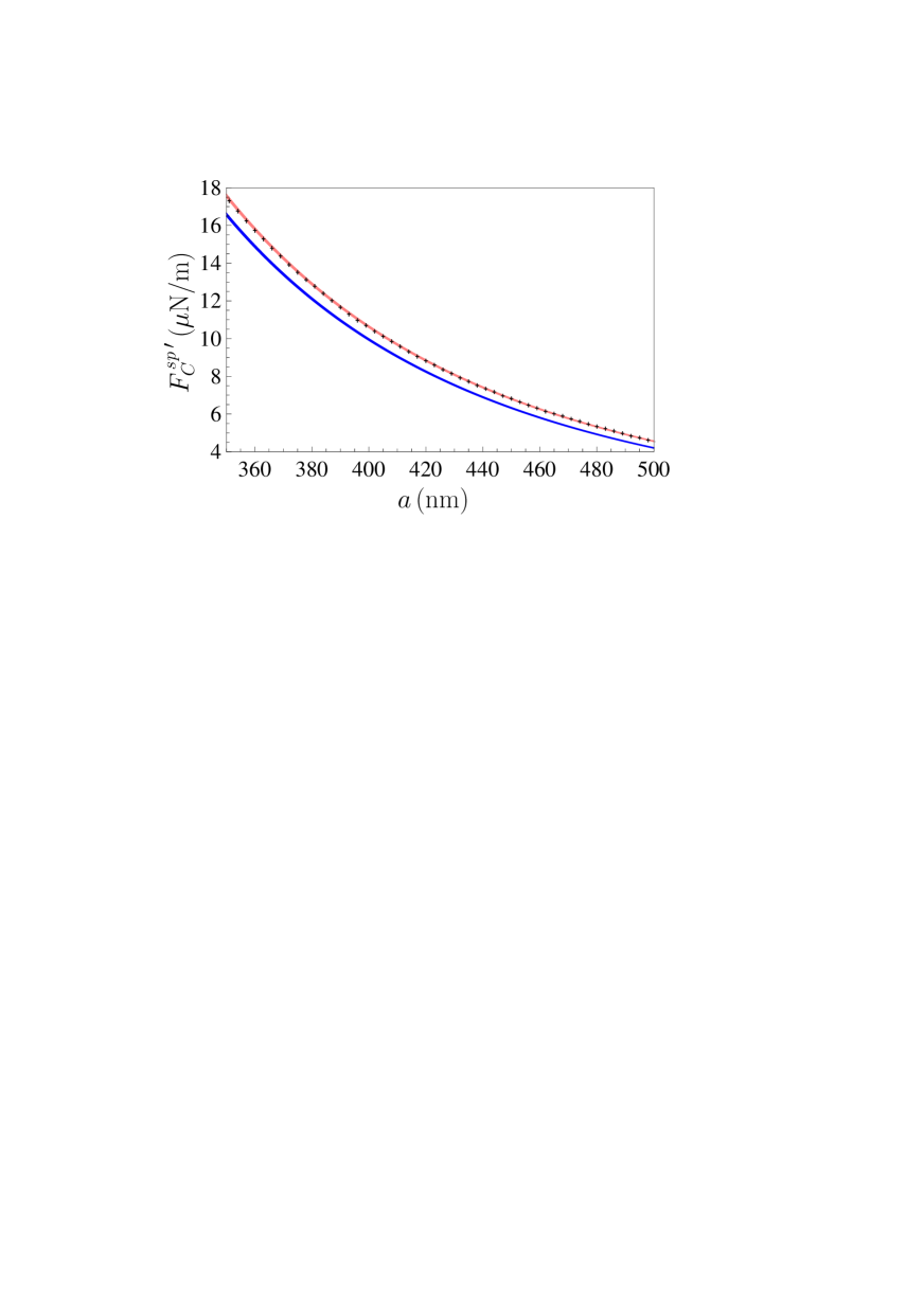
Figure 1: The mean measured gradients of the Casimir force between an Au-coated sphere and an Au-coated plate are shown by crosses as a function of separations. For clarity only each third experimental data point is plotted. The bottom and top lines demonstrate theoretical predictions of the Lifshitz theory obtained with inclusion and neglect of the relaxation of conduction electrons, respectively.

In this figure, the experimental data with their errors are shown as crosses. The bottom line shows the predictions of the Lifshitz theory obtained by using the seemingly most reliable dielectric permittivity of Au. Its behavior at relatively high frequency is found from the available optical data for the complex index of refraction of Au which is extrapolated to lower frequencies by the well tested Drude model taking into account the dissipation of free electrons. The behavior of $\varepsilon$ along the imaginary frequency axis is obtained using the Kramers-Kronig relation (see in 23 ; 24 for more details). The top line in Figure 1 shows the predictions of the Lifshitz theory obtained if the dielectric permittivity of Au given by the optical data is extrapolated to lower frequencies by the plasma model which completely disregards the relaxation properties of free electrons. From Figure 1 it is clearly seen that the top line is in a good agreement with the measurement data, whereas the bottom line is excluded by them. This result is puzzling because the plasma model is in fact applicable only at high frequencies in the region of infrared optics, where the dissipation of free electrons does not play any role. So, in our case it was used outside of its validity region. All sets of data in the experiment 22 excluded the Lifshitz theory taking the dissipation of free electrons into account over the separation range from 250 nm to $1.1~{}\mu$m.

One more representative example on the disagreement of a literally understood Lifshitz theory with the measurement data is shown in Figure 2.

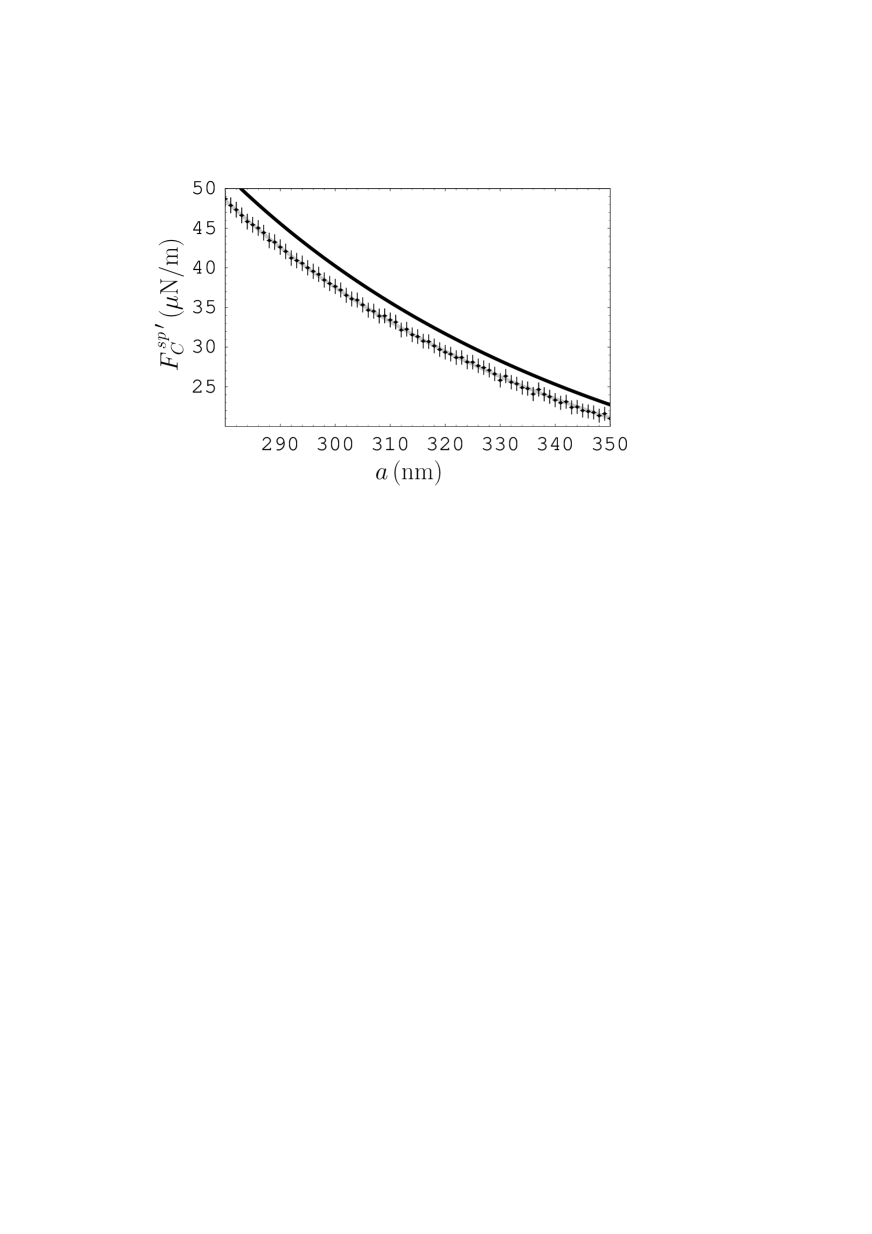
Figure 2: The mean measured gradients of the Casimir force between a Ni-coated sphere and a Ni-coated plate are shown by crosses as a function of separations. The top and bottom lines demonstrate theoretical predictions of the Lifshitz theory obtained with inclusion and neglect of the relaxation of conduction electrons, respectively.

Here, the gradient of the Casimir force between a sphere and a plate coated with the films of a magnetic metal Ni was measured 17 ; 18 . The theoretical predictions obtained with included dissipation of free electrons (i.e., using the Drude model at low frequencies) are shown by the top line, whereas the predictions found with this dissipation omitted (i.e., using the plasma model at low frequencies) are shown by the bottom line. We emphasize that for magnetic metals these lines exchange their places as compared to the nonmagnetic ones in Figure 1. As is seen in Figure 2, the theoretical predictions with taken into account dissipation of free electrons are excluded by the data. At the same time, the predictions of the Lifshitz theory disregarding this dissipation are in a good agreement with the data. We recall that similar results have been obtained in a number of experiments for metallic 11 ; 12 ; 13 ; 14 ; 15 ; 16 ; 17 ; 18 ; 19 ; 20 ; 21 ; 22 and dielectric 26 ; 27 ; 28 ; 29 ; 30 test bodies with up to a factor of 1000 differences between two alternative theoretical predictions in the experiment 19 using the differential force measurement scheme 135 ; 136 ; 137 .

Now we briefly discuss the thermodynamic problems faced by the Lifshitz theory. From Equation (2) one can easily find the Casimir entropy per unit area of the plates defined as

$$S_{C}(a,T)=-\frac{\partial{\cal F}_{C}(a,T)}{\partial T}.$$ (7)

For two semispaces made of a nonmagnetic metal with perfect crystal lattices it was proven that the Casimir entropy at zero temperature calculated using the Drude model with account of dissipation of free electrons takes the following value 32 ; 33 ; 34 :

$$S_{C}(a,0)=-\frac{k_{B}\zeta(3)}{16\pi a^{2}}\left[1-4\frac{c}{a\omega_{p}}+12\left(\frac{c}{a\omega_{p}}\right)^{2}-\ldots\right]<0,$$ (8)

where $\zeta(z)$ is the Riemann zeta function and $\omega_{p}$ is the plasma frequency.

It is seen that this value depends on the parameters of a system, such as $a$ and $\omega_{p}$, and, thus, the third law of thermodynamics (the Nernst heat theorem) is violated in this case 39 ; 40 . If, however, the dielectric permittivity of the plasma model is used, which disregards the dissipation of free electrons, one obtains 32 ; 33 ; 34

$$S_{C}(a,0)=0,$$ (9)

i.e., the Nernst heat theorem is satisfied. Similar results hold for other Casimir configurations containing metallic test bodies made of both nonmagnetic and magnetic metals 35 ; 36 ; 37 .

For dielectric semispaces the Casimir entropy at zero temperature calculated with taken into account conductivity at a constant current has the form 44 ; 45 ; 46 ; 47

$$S_{C}(a,T)=\frac{k_{B}}{16\pi a^{2}}\left\{\zeta(3)-{\rm Li}_{3}\left[\left(\frac{\varepsilon(0)-1}{\varepsilon(0)+1}\right)^{2}\right]\right\}>0,$$ (10)

where ${\rm Li}_{n}(z)$ is the polylogarithm function and $\varepsilon(0)$ is the static value of the dielectric permittivity. The right-hand side of this equation again depends on the parameters of a system which means a violation of the Nernst heat theorem. If, however, the dc conductivity is omitted in calculation, one obtains the zero value (9) of the Casimir entropy at zero temperature, i.e., the Nernst heat theorem is satisfied.

For the Casimir-Polder entropy, defined as

$$S_{CP}(a,T)=-\frac{\partial{\cal F}_{CP}(a,T)}{\partial T},$$ (11)

where ${\cal F}_{CP}$ is given in Equation (5), the situation is somewhat different. The point is that both contradictions of the Lifshitz theory with the measurement data and thermodynamics for metallic test bodies are caused by the TE contribution to the Matsubara terms with $l=0$ in Equation (2). In the Casimir-Polder free energy (5), however, the reflection coefficient ${r_{\rm TE}}(0,{k_{\bot}})$ enters with a factor $\xi_{0}^{2}=0$ and, thus, does not contribute to the result. That is why the Lifshitz theory of the Casimir-Polder interaction of a polarizable atom with a metallic plate is in agreement with thermodynamics even if the low-frequency electromagnetic response of a metal is described by the Drude model.

A different situation arises for an atom interacting with a dielectric plate. In this case the Casimir-Polder entropy at zero temperature calculated with taken into account conductivity of a plate material at a constant current (dc conductivity) is given by 45 ; 47a

$$S_{CP}(a,0)=\frac{k_{B}}{4a^{3}}\alpha(0)\frac{\varepsilon(0)-1}{\varepsilon(0)+1},$$ (12)

where $\alpha(0)$ is the static atomic polarizability. Thus, the Nernst heat theorem is violated. Later this result was generalized for a magnetizable atom and a ferromagnetic dielectric plate 48 . If, however, the dc conductivity of a plate material is omitted in calculations, one obtains in place of (12)

$$S_{CP}(a,0)=0,$$ (13)

i.e., the Nernst heat theorem is satisfied 45 ; 47a ; 48 . We emphasize that in the single precise experiment on measuring the Casimir-Polder force at separations of a few micrometers 30 , where the difference between alternative theoretical predictions of the Lifshitz theory is relatively large, the measurement data were found in agreement with theory disregarding the dc conductivity 30 and exclude the theory taking the dc conductivity into account 27 . This situation again presents a puzzle or, as it is also called, a conundrum 111a because the dc conductivity of dielectrics at nonzero temperature is an observable and well studied physical effect, so that there is no reason why one should omit it when comparing experiment with theory.

In the end of this section, we note that the violation of the Nernst heat theorem and the disagreement between the measured Casimir and Casimir-Polder forces and predictions of the Lifshitz theory with included dc conductivity of a dielectric plate are again caused by the term with $l=0$ in Equations (2) and (5). Here, however, this happens due to the TM contribution to Equations (2) and (5) as opposed to the case of Casimir interaction between two metallic plates where similar effects are caused by the TE contribution to Equation (2).

4 Different Approaches to Theoretical Description of the Electromagnetic Response of Graphene

As was explained in Section 2, the Casimir interaction between two planar structures, as well as between an atom and a planar structure, can be described by Equations (2) and (5), respectively, if the reflection coefficients on a planar structure are defined appropriately. Thus, Equations (2) and (5) are applicable for theoretical description of the Casimir interaction between two graphene sheets, as well as of the Casimir-Polder interaction between an atom and a graphene sheet. This raises a question of what is the form of the reflection coefficients on a graphene sheet. The point is that the standard Fresnel coefficients (3) or their generalizations for the plates of finite thickness 24 are expressed via the frequency-dependent dielectric permittivity which is well defined only for volumetric bodies containing sufficiently large number of atomic layers. This condition is not satisfied for graphene which is a one-atom thick layer of carbon atoms 49 ; 50 ; 51 .

As a first approximation, graphene was treated as a two-dimensional free-electron gas characterized by some typical wave number $K=6.75\times 10^{5}~{}\mbox{m}^{-1}$ which is determined by the hexagonal structure of graphite 67 ; 68 . The reflection coefficients of the electromagnetic waves on such a sheet take the form 67 ; 68 ; 138

$${r_{\rm TM}}({{\rm i}\xi_{l},k_{\bot}})=\frac{c^{2}q_{l}K}{c^{2}q_{l}K+\xi_{l}^{2}},\qquad{r_{\rm TE}}({{\rm i}\xi_{l},k_{\bot}})=-\frac{K}{K+q_{l}}.$$ (14)

Equations (2) and (5) with the reflection coefficients (14) were used to calculate the Casimir and Casimir-Polder interactions in various carbon nanostructures 65 ; 67 ; 68 ; 69 ; 70 ; 138 ; 139 . It should be taken into account, however, that the plasma-sheet approach, which is also often called "the hydrodynamic model", fails to account for a linearity of the dispersion relation for graphene. Finally, it was demonstrated that the theoretical predictions of this approach are in contradiction 140 with the experimental data on measuring the Casimir force in graphene systems 123 .

In the widely used approach, the reflection coefficients on a graphene sheet are expressed via the longitudinal, $\chi^{\|}({{\rm i}\xi_{l},k_{\bot}})$, and transverse, $\chi^{\bot}({{\rm i}\xi_{l},k_{\bot}})$, density-density correlation functions of graphene 82 ; 141 ; 142

$${r_{\rm TM}}({{\rm i}\xi_{l},k_{\bot}})=\frac{2\pi e^{2}q_{l}\chi^{\|}({{\rm i}\xi_{l},k_{\bot}})}{2\pi e^{2}q_{l}\chi^{\|}({{\rm i}\xi_{l},k_{\bot}})-{k_{\bot}^{2}}},\qquad{r_{\rm TE}}({{\rm i}\xi_{l},k_{\bot}})=-\frac{2\pi e^{2}\xi_{l}^{2}\chi^{\bot}({{\rm i}\xi_{l},k_{\bot}})}{2\pi e^{2}\xi_{l}^{2}\chi^{\bot}({{\rm i}\xi_{l},k_{\bot}})-c^{2}{k_{\bot}^{2}}q_{l}}.$$ (15)

The density-density correlation functions are connected with the nonlocal electric susceptibilities (polarizabilities) of graphene by $\chi^{\|,\bot}=-{k_{\bot}}\alpha^{\|,\bot}/(2\pi e^{2})$. The density-density correlation functions have been used in computations of the Casimir force 63 ; 76 ; 79 ; 80 ; 82 . It should be noted, however, that although the formulas (15) are exact, the exact expressions for the correlation functions $\chi^{\|,\bot}$ at nonzero temperature remain unknown with exception of only some particular cases.

In a similar way, the reflection coefficients on a graphene sheet were expressed via the in-plane, $\sigma^{\|}({{\rm i}\xi_{l},k_{\bot}})$, and out-of-plane, $\sigma^{\bot}({{\rm i}\xi_{l},k_{\bot}})$, electrical conductivities of graphene 79 ; 82

$${r_{\rm TM}}({{\rm i}\xi_{l},k_{\bot}})=\frac{2\pi q_{l}\sigma^{\|}({{\rm i}\xi_{l},k_{\bot}})}{2\pi q_{l}\sigma^{\|}({{\rm i}\xi_{l},k_{\bot}})+\xi_{l}},\qquad{r_{\rm TE}}({{\rm i}\xi_{l},k_{\bot}})=-\frac{2\pi\xi_{l}\sigma^{\bot}({{\rm i}\xi_{l},k_{\bot}})}{2\pi\xi_{l}\sigma^{\bot}({{\rm i}\xi_{l},k_{\bot}})+c^{2}q_{l}}.$$ (16)

These expressipons are also exact because the conductivities are expressed via the density-density correlation functions as $\sigma^{\|,\bot}=-e^{2}\xi_{l}\chi^{\|,\bot}/{k_{\bot}}^{2}$ 82 . In doing so, the exact expressions for the conductivities of graphene at nonzero temperature also remained unknown. Thus, the Casimir force between two graphene sheets was computed under an assumption that the graphene conductivity can be modeled by the in-plane optical conductivity of graphite with no account 77 or with account 81 of spatial dispersion. This modeling includes the two-dimensional Drude term and a series of Lorentz oscillators.

By and large several approximate methods for calculation of the Casimir interaction have been elaborated but their accuracy and the region of applicability remained uncertain.

5 Quantum Field Theoretical Description of the Electromagnetic Response of Graphene via the Polarization Tensor

As mentioned in Section 1, the field of massless or having some small mass $m$ electronic excitations in graphene satisfy the three-dimensional Dirac equation where the speed of light $c$ is replaced with the Fermi velocity $v_{F}$. For graphene possessing the chemical potential $\mu$ this equation takes the form 94 ; 143

$$\left[\frac{\gamma^{0}}{v_{F}}\left({{\rm i}}\hbar\frac{\partial}{\partial t}-\mu\right)+{{\rm i}}\hbar\left(\gamma^{1}\frac{\partial}{\partial x^{1}}+\gamma^{2}\frac{\partial}{\partial x^{2}}\right)-mv_{F}\right]\psi(x)=0,$$ (17)

where the Dirac matrices satisfy the conditions $(\gamma^{0})^{2}=-(\gamma^{1,2})^{2}=1$.

Multiplying this equation by the dimensionless Fermi velocity ${\tilde{v}_{F}}=v_{F}/c\approx 1/300$, we can rewrite it in the form

$$\left[\frac{{\tilde{\gamma}}^{0}}{c}\left({{\rm i}}\hbar\frac{\partial}{\partial t}-\mu\right)+{{\rm i}}\hbar\left({\tilde{\gamma}}^{1}\frac{\partial}{\partial x^{1}}+{\tilde{\gamma}}^{2}\frac{\partial}{\partial x^{2}}\right)-mc{\tilde{v}_{F}}^{2}\right]\psi(x)=0,$$ (18)

where ${\tilde{\gamma}}^{0}=\gamma^{0}$ and ${\tilde{\gamma}}^{1,2}={\tilde{v}_{F}}\gamma^{1,2}$. Note that $2mv_{F}^{2}=\Delta$, where $\Delta$ is the energy gap, so that $mc{\tilde{v}_{F}}^{2}=\Delta/(2c)$. Then, an interaction with the electromagnetic field $A_{\beta}(x)$ is introduced by the replacement

$${{\rm i}}\hbar\frac{\partial}{\partial x^{\beta}}\to{{\rm i}}\hbar\frac{\partial}{\partial x^{\beta}}-\frac{e}{c}A_{\beta}(x),$$ (19)

where $x^{\beta}=(ct,x^{1},x^{2})$. As a result, the Dirac equation (18) is given by

$$\left[{\tilde{\gamma}}^{0}\left({{\rm i}}\hbar\frac{\partial}{\partial t}-eA_{0}-\mu\right)+{\tilde{\gamma}}^{1}\left({{\rm i}}\hbar c\frac{\partial}{\partial x^{1}}-eA_{1}\right)+{\tilde{\gamma}}^{2}\left({{\rm i}}\hbar c\frac{\partial}{\partial x^{2}}-eA_{2}\right)-\frac{\Delta}{2}\right]\psi(x)=0.$$ (20)

In the one-loop approximation, an interaction of the graphene quasiparticles with the electromagnetic field is described by the diagram consisting of an electronic quasiparticle loop with two photon legs. At zero temperature this corresponds to the following expression for the polarization tensor 94 ; 144

$$\Pi^{\beta\delta}(k_{0},\mbox{\boldmath$k_{\bot}$})={{\rm i}}\frac{e^{2}}{c}\int\frac{dq_{0}\,d^{2}\mbox{\boldmath$q_{\bot}$}}{(2\pi)^{3}}{\rm tr}\left[S(q_{0},\mbox{\boldmath$q_{\bot}$}){\tilde{\gamma}}^{\beta}S(q_{0}-k_{0},\mbox{\boldmath$q_{\bot}$}-\mbox{\boldmath$k_{\bot}$}){\tilde{\gamma}}^{\delta}\right],$$ (21)

where $(q_{0},\mbox{\boldmath$q_{\bot}$})$ and $(k_{0},\mbox{\boldmath$k_{\bot}$})$ are the three-dimensional wave vectors of a loop electronic excitation and an external photon, respectively, and the propagator of the quasiparticles takes the form 94

$$S(q_{0},\mbox{\boldmath$q_{\bot}$})=-\frac{{\tilde{\gamma}}^{0}[q_{0}+\mu/(\hbar c)]-{\tilde{\gamma}}^{1}q_{1}-{\tilde{\gamma}}^{2}q_{2}-\Delta/(2\hbar c)}{[q_{0}+\mu/(\hbar c)+{{\rm i}}\,\epsilon\,{\rm sign}q_{0}]^{2}-{\tilde{v}_{F}}^{2}{\mbox{\boldmath$q$}_{\bot}^{2}}-\Delta^{2}/(4\hbar^{2}c^{2})}.$$ (22)

For taking into account nonzero temperature in the framework of the Matsubara formalism, one should replace an integration with respect to $q_{0}$ in (21) with a summation over the pure imaginary fermionic Matsubara frequencies given by

$$cq_{0n}=2\pi{{\rm i}}\left(n+\frac{1}{2}\right)\frac{k_{B}T}{\hbar},$$ (23)

where $n=\pm 1,\,\pm 2,\,\ldots\,$. One should also put $k_{0l}={{\rm i}}\xi_{l}/c$, where $\xi_{l}$ are the bosonic Matsubara frequencies. Taking into account that there are four fermionic species for graphene, the polarization tensor (21) is expressed as

$$\Pi^{\beta\delta}(k_{0l},\mbox{\boldmath$k_{\bot}$})=-8\pi\alpha k_{B}T\sum_{n=-\infty}^{\infty}\left(n+\frac{1}{2}\right)\int\frac{\,d^{2}\mbox{\boldmath$q_{\bot}$}}{(2\pi)^{2}}{\rm tr}\left[S(q_{0n},\mbox{\boldmath$q_{\bot}$}){\tilde{\gamma}}^{\beta}S(q_{0n}-k_{0l},\mbox{\boldmath$q_{\bot}$}-\mbox{\boldmath$k_{\bot}$}){\tilde{\gamma}}^{\delta}\right].$$ (24)

Explicit expressions for this tensor which can be analytically continued over the entire plane of complex frequencies were found in 105 ; 106 . They are the functions of the Matsubara frequencies, magnitude of the photon wave vector, temperature, energy gap and chemical potential. In fact the polarization tensor in a medium is completely defined by the two independent quantities, e.g., $\Pi_{00}$ and $\Pi_{\beta}^{\,\beta}$ 94 . For our purposes, instead of a trace, it is more convenient to exploit

$$\Pi({{\rm i}\xi_{l},k_{\bot}})\equiv{k_{\bot}^{2}}\Pi_{\beta}^{\,\beta}({{\rm i}\xi_{l},k_{\bot}})-q_{l}^{2}\Pi_{00}({{\rm i}\xi_{l},k_{\bot}})$$ (25)

as the second quantity. Below we use the abbreviate notations

$$\Pi_{00}({{\rm i}\xi_{l},k_{\bot}})\equiv\Pi_{00,l},\qquad\Pi({{\rm i}\xi_{l},k_{\bot}})\equiv\Pi_{l},$$ (26)

and write out all or some of the arguments ${{\rm i}\xi_{l},k_{\bot}},T,\Delta$, and $\mu$ where it is helpful for better understanding.

We present the explicit expressions for the following two contributions to $\Pi_{00,l}$ and $\Pi_{l}$:

$$\Pi_{00}({{\rm i}\xi_{l},k_{\bot}},T,\Delta,\mu)=\Pi_{00}^{(0)}({{\rm i}\xi_{l},k_{\bot}},\Delta)+\Pi_{00}^{(1)}({{\rm i}\xi_{l},k_{\bot}},T,\Delta,\mu),$$

$$\Pi({{\rm i}\xi_{l},k_{\bot}},T,\Delta,\mu)=\Pi^{(0)}({{\rm i}\xi_{l},k_{\bot}},\Delta)+\Pi^{(1)}({{\rm i}\xi_{l},k_{\bot}},T,\Delta,\mu).$$ (27)

Here, the quantities $\Pi_{00}^{(0)}$ and $\Pi^{(0)}$ describe the undoped graphene with $\mu=0$ but, generally speaking, $\Delta\neq 0$ at zero temperature. They are given by 93

$$\Pi_{00,l}^{(0)}=\frac{\alpha\hbar c{{k_{\bot}^{2}}}}{p_{l}}\Psi(D_{l}),\qquad\Pi_{l}^{(0)}=\alpha\hbar{{k_{\bot}^{2}}}\frac{p_{l}}{c}\Psi(D_{l}),$$ (28)

where $p_{l}^{2}=v_{F}^{2}{{k_{\bot}^{2}}}+\xi_{l}^{2}$, $D_{l}=\Delta/(\hbar p_{l})$ and

$$\Psi(x)=2\left[x+(1-x^{2})\arctan(x^{-1})\right].$$ (29)

The quantities $\Pi_{00}^{(1)}$ and $\Pi^{(1)}$ in (27) describe both the thermal effect and the dependence on $\mu$. They can be presented in the form 105 ; 106 ; 110

$$\Pi_{00,l}^{(1)}=\frac{4\alpha\hbar cp_{l}}{v_{F}^{2}}\int_{D_{l}}^{\infty}\!\!\!du\left(\frac{1}{e^{B_{l}u+\frac{\mu}{k_{B}T}}+1}+\frac{1}{e^{B_{l}u-\frac{\mu}{k_{B}T}}+1}\right)$$

$$~{}~{}~{}~{}~{}~{}~{}~{}~{}~{}~{}~{}~{}~{}~{}~{}~{}~{}~{}~{}~{}~{}~{}~{}~{}~{}~{}~{}~{}~{}\times\left[1-{\rm Re}\frac{1-u^{2}+2{{\rm i}}\frac{\xi_{l}}{p_{l}}u}{\left(1-u^{2}+2{{\rm i}}\frac{\xi_{l}}{p_{l}}u+\frac{v_{F}^{2}{{k_{\bot}^{2}}}}{p_{l}^{2}}D_{l}^{2}\right)^{1/2}}\right],$$

$$\Pi_{l}^{(1)}=-\frac{4\alpha\hbar p_{l}\xi_{l}^{2}}{cv_{F}^{2}}\int_{D_{l}}^{\infty}\!\!\!du\left(\frac{1}{e^{B_{l}u+\frac{\mu}{k_{B}T}}+1}+\frac{1}{e^{B_{l}u-\frac{\mu}{k_{B}T}}+1}\right)$$

$$~{}~{}~{}~{}~{}~{}~{}~{}~{}~{}~{}~{}~{}~{}~{}~{}~{}~{}~{}~{}~{}~{}~{}~{}~{}~{}~{}~{}~{}~{}\times\left[1-{\rm Re}\frac{1-\frac{p_{l}^{2}}{\xi_{l}^{2}}u^{2}+2{{\rm i}}\frac{p_{l}}{\xi_{l}}u+\frac{v_{F}^{2}{{k_{\bot}^{2}}}}{\xi_{l}^{2}}D_{l}^{2}}{\left(1-u^{2}+2{{\rm i}}\frac{\xi_{l}}{p_{l}}u+\frac{v_{F}^{2}{{k_{\bot}^{2}}}}{p_{l}^{2}}D_{l}^{2}\right)^{1/2}}\right],$$ (30)

where $B_{l}=\hbar p_{l}/(2k_{B}T)$.

In order to investigate one specific case, which was not considered in the literature so far, we also need the expressions for $\Pi_{00,l}$ and $\Pi_{l}$ at $T=0$ calculated under the condition $\Delta<2\mu$. They were obtained in 110 by using Equations (27)–(29) and (30) taken at $T=0$. The result is

$$\Pi_{00}({{\rm i}\xi_{l},k_{\bot}},0,\Delta,\mu)=\frac{8\alpha c\mu}{v_{F}^{2}}-\frac{\alpha c\hbar{{k_{\bot}^{2}}}}{p_{l}}\left\{2M_{l}{\rm Im}(y_{l}\sqrt{1+y_{l}^{2}})\right.$$

$$~{}~{}~{}~{}~{}~{}~{}~{}~{}~{}~{}~{}~{}~{}~{}~{}~{}~{}~{}~{}~{}~{}~{}~{}~{}~{}~{}~{}~{}~{}\left.+(2-M_{l})\left[2{\rm Im}\ln(y_{l}+\sqrt{1+y_{l}^{2}})-\pi\right]\right\},$$

$$\Pi({{\rm i}\xi_{l},k_{\bot}},0,\Delta,\mu)=-\frac{8\alpha\xi_{l}^{2}\mu}{cv_{F}^{2}}+\frac{\alpha\hbar p_{l}{{k_{\bot}^{2}}}}{c}\left\{2M_{l}{\rm Im}(y_{l}\sqrt{1+y_{l}^{2}})\right.$$

$$~{}~{}~{}~{}~{}~{}~{}~{}~{}~{}~{}~{}~{}~{}~{}~{}~{}~{}~{}~{}~{}~{}~{}~{}~{}~{}~{}~{}~{}~{}\left.-(2-M_{l})\left[2{\rm Im}\ln(y_{l}+\sqrt{1+y_{l}^{2}})-\pi\right]\right\},$$ (31)

where the following notations are introduced

$$M_{l}=1+D_{l}^{2},\qquad y_{l}\equiv y_{l}(\Delta,\mu)=\frac{\hbar\xi_{l}+2{{\rm i}}\mu}{\hbar v_{F}{k_{\bot}}\sqrt{M_{l}}}.$$ (32)

The reflection coefficients on a graphene sheet can be expressed in terms of the polarization tensor given by Equations (27)–(30) 94

$${r_{\rm TM}}({{\rm i}\xi_{l},k_{\bot}})=\frac{q_{l}\Pi_{00}({{\rm i}\xi_{l},k_{\bot}})}{q_{l}\Pi_{00}({{\rm i}\xi_{l},k_{\bot}})+2\hbar{{k_{\bot}^{2}}}},\qquad{r_{\rm TE}}({{\rm i}\xi_{l},k_{\bot}})=-\frac{\Pi({{\rm i}\xi_{l},k_{\bot}})}{\Pi({{\rm i}\xi_{l},k_{\bot}})+2\hbar{{k_{\bot}^{2}}}q_{l}}.$$ (33)

Taking into account a connection between the polarization tensor and density-density correlation functions 104

$$\chi^{\|}({{\rm i}\xi_{l},k_{\bot}})=-\frac{1}{4\pi e^{2}\hbar}\Pi_{00}({{\rm i}\xi_{l},k_{\bot}}),\qquad\chi^{\bot}({{\rm i}\xi_{l},k_{\bot}})=-\frac{c^{2}}{4\pi e^{2}\hbar\xi_{l}^{2}}\Pi({{\rm i}\xi_{l},k_{\bot}}),$$ (34)

the reflection coefficients (33) become equivalent to (15). Thus, calculation of explicit expressions (27)–(30) for the polarization tensor of graphene at any $T$ and with any values of $\Delta$ and $\mu$ on the basis of first principles of thermal quantum field theory resulted in respective expressions for the density-density correlation functions which were previously available only in some specific cases.

Equations (27)–(30) have been used in calculations of the Casimir interaction in graphene systems 107 ; 108 ; 109 ; 110 ; 111 ; 111a . After an analytic continuation to the real frequency axis, they were also applied for investigation of the electrical conductivity 112 ; 113 ; 114 ; 115 and reflectances of graphene 116 ; 117 ; 118 ; 119 ; 120 ; 121 . This allows to compare the longitudinal and transverse dielectric permittivities of graphene $\varepsilon^{\|,\bot}$, which are directly expressed via the respective conductivities $\sigma^{\|,\bot}$, with the dielectric permittivity of the Drude model $\varepsilon_{D}$. As shown in 114 , for $\hbar\omega<\Delta$ it holds ${\rm Re}\,\sigma^{\|,\bot}=0$. This results in ${\rm Im}\,\varepsilon^{\|,\bot}=0$ unlike the Drude model for which ${\rm Im}\,\varepsilon_{D}\sim 1/\omega$ when $\omega$ goes to zero, but similar to the plasma model for which ${\rm Im}\,\varepsilon_{p}=0$. The imaginary part of $\sigma^{\|,\bot}$ for graphene is contained in equation (47) of 114 . In the asymptotic limit $\omega\to 0$, for both cases $\Delta>2\mu$ and $\Delta<2\mu$ it was shown that ${\rm Im}\,\sigma^{\|,\bot}\sim 1/\omega$ (see equations (50) and (54) in 114 ) which results in ${\rm Re}\,\varepsilon^{\|,\bot}\sim-1/\omega^{2}$. This is again unlike the Drude model for which ${\rm Re}\,\varepsilon_{D}$ takes a finite value at $\omega=0$, but in direct analogy to the plasma model which does not take into account the relaxation properties of free electrons (see Section 3). Thus, the dielectric properties of graphene, expressed via the polarization tensor, provide reason enough to guess that the Casimir entropy calculated using the reflection coefficients (33) satisfies the Nernst heat theorem like it holds for the reflection coefficients (3) and the dielectric permittivity of the plasma model.

Below we discuss an application of the polarization tensor for a treatment of thermodynamic properties of the Casimir-Polder and Casimir interactions in graphene systems and make sure that this guess is correct.

6 Low-Temperature Behavior of the Casimir-Polder Free Energy and Entropy for an Atom and a Pristine Graphene Sheet

The asymptotic behavior of the free energy for an atom interacting with a sheet of ideal graphene possessing $\Delta=\mu=0$ at low $T$ was investigated using the formalism of the polarization tensor 145 . The Casimir-Polder free energy was expressed according to (5) and the reflection coefficients presented in (33). In this case, the polarization tensor was significantly simplified by putting $\Delta=\mu=0$ in Equations (27)–(32).

The main idea of the perturbation approach used in 145 is to present the polarization tensor as a sum of two contributions (27), where for a pristine graphene with $\Delta=\mu=0$ the quantities $\Pi_{00,l}^{(1)}$ and $\Pi_{l}^{(1)}$ have the meaning of the thermal corrections, and to make an expansion in powers of the small parameters

$$\frac{\Pi_{00,l}^{(1)}}{\Pi_{00,l}^{(0)}}\ll 1,\qquad\frac{\Pi_{l}^{(1)}}{\Pi_{l}^{(0)}}\ll 1.$$ (35)

The smallness of these parameters is guaranteed by the fact that their numerators go to zero with vanishing temperature, whereas denominators are equal to the nonvanishing quantities $\Pi_{00}{({\rm i}\xi_{l},k_{\bot},0)}$ and $\Pi{({\rm i}\xi_{l},k_{\bot},0)}$ in the case of a pristine graphene.

As a result, the reflection coefficients (33) are presented as a sum of the contributions at zero temperature and the thermal corrections to them

$$r_{\rm TM,TE}({{\rm i}\xi_{l},k_{\bot}})=r_{\rm TM,TE}^{(0)}({{\rm i}\xi_{l},k_{\bot}})+{\delta_{T}}r_{\rm TM,TE}({{\rm i}\xi_{l},k_{\bot}}).$$ (36)

Here, the first contributions on the right-hand side are given by (33) where, instead $\Pi_{00,l}$ and $\Pi_{l}$, we substitute $\Pi_{00,l}^{(0)}$ and $\Pi_{l}^{(0)}$ defined in (28) but with $\Delta=0$:

$${r_{\rm TM}^{(0)}}({{\rm i}\xi_{l},k_{\bot}})=\frac{\alpha\pi cq_{l}}{\alpha\pi cq_{l}+2p_{l}},\qquad{r_{\rm TE}^{(0)}}({{\rm i}\xi_{l},k_{\bot}})=-\frac{\alpha\pi p_{l}}{\alpha\pi p_{l}+2cq_{l}}.$$ (37)

The second contributions to (36) are expressed as

$${\delta_{T}}{r_{\rm TM}}({{\rm i}\xi_{l},k_{\bot}})=\frac{2\alpha\pi cq_{l}p_{l}}{(\alpha\pi cq_{l}+2p_{l})^{2}}\,\frac{\Pi_{00,l}^{(1)}}{\Pi_{00,l}^{(0)}},\qquad{\delta_{T}}{r_{\rm TE}}({{\rm i}\xi_{l},k_{\bot}})=-\frac{2\alpha\pi cq_{l}p_{l}}{(\alpha\pi p_{l}+2cq_{l})^{2}}\,\frac{\Pi_{l}^{(1)}}{\Pi_{l}^{(0)}},$$ (38)

where $\Pi_{00,l}^{(1)}$ and $\Pi_{l}^{(1)}$ are defined by (30) with $\Delta=\mu=0$.

Now we note that the temperature-dependent part of the Casimir-Polder free energy can be presented as

$${\delta_{T}}{\cal F}_{CP}(a,T)={\cal F}_{CP}(a,T)-E_{CP}(a),$$ (39)

where ${\cal F}_{CP}$ is presented in (5) and the Casimir-Polder energy at $T=0$ is given by

$${E}_{CP}(a)=-\frac{\hbar}{2\pi}\int_{0}^{\infty}\!\!\!d\xi\alpha({{\rm i}}\xi)\int_{0}^{\infty}\!\!{k_{\bot}}d{k_{\bot}}qe^{-2aq}\left[\left(2-\frac{\xi^{2}}{q^{2}c^{2}}\right){r_{\rm TM}^{(0)}}({{\rm i}}\xi,{k_{\bot}})-\frac{\xi^{2}}{q^{2}c^{2}}{r_{\rm TE}^{(0)}}({{\rm i}}\xi,{k_{\bot}})\right],$$ (40)

where $q^{2}={{k_{\bot}^{2}}}+\xi^{2}/c^{2}$.

Substituting Equation (36) in the Casimir-Polder free energy (5), the thermal correction to the Casimir-Polder energy $E_{CP}$ can be identically presented as

$${\delta_{T}}{\cal F}_{CP}(a,T)={\delta_{T}^{\rm impl}}{\cal F}_{CP}(a,T)+{\delta_{T\!}^{\rm expl}\,}{\cal F}_{CP}(a,T),$$ (41)

where the contributions to the right-hand side of this equation are defined as

$${\delta_{T}^{\rm impl}}{\cal F}_{CP}(a,T)=-k_{B}T\sum_{l=0}^{\infty}{\vphantom{\sum}}^{\!\prime}\alpha({{\rm i}}\xi_{l})\int_{0}^{\infty}\!\!{k_{\bot}}d{k_{\bot}}q_{l}e^{-2aq_{l}}$$

$$~{}~{}~{}~{}\times\left[\left(2-\frac{\xi_{l}^{2}}{q_{l}^{2}c^{2}}\right){r_{\rm TM}^{(0)}}({{\rm i}\xi_{l},k_{\bot}})-\frac{\xi_{l}^{2}}{q_{l}^{2}c^{2}}{r_{\rm TE}^{(0)}}({{\rm i}\xi_{l},k_{\bot}})\right]-E_{CP}(a)$$ (42)

and

$${\delta_{T\!}^{\rm expl}\,}{\cal F}_{CP}(a,T)=-k_{B}T\sum_{l=0}^{\infty}{\vphantom{\sum}}^{\!\prime}\alpha({{\rm i}}\xi_{l})\int_{0}^{\infty}\!\!{k_{\bot}}d{k_{\bot}}q_{l}e^{-2aq_{l}}$$

$$~{}~{}~{}~{}~{}~{}~{}~{}~{}~{}~{}~{}~{}~{}~{}\times\left[\left(2-\frac{\xi_{l}^{2}}{q_{l}^{2}c^{2}}\right){\delta_{T}}{r_{\rm TM}}({{\rm i}\xi_{l},k_{\bot}})-\frac{\xi_{l}^{2}}{q_{l}^{2}c^{2}}{\delta_{T}}{r_{\rm TE}}({{\rm i}\xi_{l},k_{\bot}})\right].$$ (43)

Here, ${\delta_{T}^{\rm impl}}{\cal F}_{CP}$ contains the reflection coefficients at $T=0$, so that its dependence on $T$ originates from only the Matsubara summation. This is the reason why it is called "implicit". The contribution ${\delta_{T\!}^{\rm expl}\,}{\cal F}_{CP}$ would be equal to zero for the reflection coefficients independent on $T$ as a parameter. Because of this it called "explicit".

It is convenient also to split ${\delta_{T\!}^{\rm expl}\,}{\cal F}_{CP}$ in two parts

$${\delta_{T\!}^{\rm expl}\,}{\cal F}_{CP}(a,T)={\delta_{T\!,\,l=0}^{\rm expl}\,}{\cal F}_{CP}(a,T)+{\delta_{T\!,\,l\geqslant 1}^{\rm expl}\,}{\cal F}_{CP}(a,T),$$ (44)

where the first part is equal to the term of (43) with $l=0$ and the second part is equal to the sum of all remaining terms with $l\geqslant 1$.

As is seen from Equations (40) and (42), the implicit thermal correction ${\delta_{T}^{\rm impl}}{\cal F}_{CP}$ is represented by a difference between the sum and the integral which can be calculated by using the Abel-Plana formula 24 ; 146

$$\sum_{l=0}^{\infty}{\vphantom{\sum}}^{\!\prime}F(l)-\int_{0}^{\infty}\!\!\!F(t)dt={{\rm i}}\int_{0}^{\infty}\!\frac{F({{\rm i}}t)-F(-{{\rm i}}t)}{e^{2\pi t}-1}dt,$$ (45)

which is valid for a function $F(z)$ analytic in the right half-plane.

Using this approach, it was shown that at sufficiently low temperature satisfying the condition $k_{B}T\ll\hbar v_{F}/(2a)$ the implicit thermal correction decreases with temperature as (see 145 for details)

$${\delta_{T}^{\rm impl}}{\cal F}_{CP}(a,T)\sim-\frac{\alpha_{0}(k_{B}T)^{4}}{(\hbar c)^{3}},$$ (46)

where $\alpha_{0}=\alpha(0)$ is the static atomic polarizability. Here and below we preserve only dimensional parameters in the asymptotic formulas. This behavior is determined by the TM contribution to the Casimir-Polder free energy. The result (46) is similar to that for an atom interacting with a dielectric plate 24 ; 45 .

Now we deal with the first part of the explicit thermal correction, ${\delta_{T\!,\,l=0}^{\rm expl}\,}{\cal F}_{CP}$, given by the term with $l=0$ in (43). It is determined by only the TM mode because $\xi_{0}=0$. In this case the derivation of the asymptotic expression at low $T$ results in 145

$${\delta_{T\!,\,l=0}^{\rm expl}\,}{\cal F}_{CP}(a,T)\sim\frac{\alpha_{0}(k_{B}T)^{4}}{(\hbar c)^{3}}\ln\frac{ak_{B}T}{\hbar v_{F}}.$$ (47)

One can see that (47) becomes greater in magnitude that the magnitude of (46) with decreasing $T$.

The last contribution to the thermal correction is the second part of (44), ${\delta_{T\!,\,l\geqslant 1}^{\rm expl}\,}{\cal F}_{CP}$, which is equal to the sum of all terms of (43) with $l\geqslant 1$. The asymptotic behavior of this part at low $T$ can be found taking into account that the major contribution to the integral with respect to ${k_{\bot}}$ in (43) is given by ${k_{\bot}}$ satisfying the condition $q_{l}\sim 1/(2a)$. Then at sufficiently low temperature $k_{B}T\ll\hbar v_{F}/(2a)$, one arrives at 145

$${\delta_{T\!,\,l\geqslant 1}^{\rm expl}\,}{\cal F}_{CP}(a,T)\sim-\frac{\alpha_{0}(k_{B}T)^{3}}{v_{F}^{2}\hbar^{2}a}.$$ (48)

This goes to zero slower than (46) and (47) and is again determined by the TM reflection coefficient.

One can conclude that for an atom interacting with a pristine graphene sheet the thermal correction (39) to the Casimir-Polder energy behaves at low temperature as

$${\delta_{T}}{\cal F}_{CP}(a,T)\sim{\delta_{T\!,\,l\geqslant 1}^{\rm expl}\,}{\cal F}_{CP}(a,T)\sim-\frac{\alpha_{0}(k_{B}T)^{3}}{v_{F}^{2}\hbar^{2}a}.$$ (49)

The resulting Casimir-Polder entropy vanishes with vanishing temperature by the power law

$$S_{CP}(a,T)\sim\frac{\alpha_{0}k_{B}(k_{B}T)^{2}}{v_{F}^{2}\hbar^{2}a}.$$ (50)

This means that the Lifshitz theory of atom-graphene interaction using the reflection coefficients expressed via the polarization tensor satisfies the requirements of thermodynamics for a pristine graphene.

The asymptotic results (49) and (50) obtained for a pristine graphene are presented in column 2 of Table 1 (lines 2 and 3, respectively).

Table 1: Up to an order of magnitude asymptotic behaviors at arbitrarily low temperature of the thermal corrections to the Casimir-Polder energy (line 2) and of the Casimir-Polder entropy (line 3) under different relationships between the energy gap $\Delta$ and chemical potential $\mu$ (line 1).

	$\Delta=\mu=0$	$\Delta>2\mu\geqslant 0$	$\Delta=2\mu\neq 0$	$0\leqslant\Delta<2\mu$
${\delta_{T}}{\cal F}_{CP}(a,T)$	$-\frac{\alpha_{0}(k_{B}T)^{3}}{v_{F}^{2}\hbar^{2}a}$	$-\frac{\alpha_{0}(k_{B}T)^{5}}{(\hbar c)^{3}\Delta}$	$-\frac{\alpha_{0}k_{B}T}{a^{3}}$	$-\frac{\alpha_{0}\mu^{2}(k_{B}T)^{2}}{(\hbar c)^{2}a\sqrt{4\mu^{2}-\Delta^{2}}}$
$S_{CP}(a,T)$	$\frac{\alpha_{0}k_{B}(k_{B}T)^{2}}{v_{F}^{2}\hbar^{2}a}$	$\frac{\alpha_{0}k_{B}(k_{B}T)^{4}}{(\hbar c)^{3}\Delta}$	$\frac{\alpha_{0}k_{B}}{a^{3}}$	$\frac{\alpha_{0}\mu^{2}k_{B}^{2}T}{(\hbar c)^{2}a\sqrt{4\mu^{2}-\Delta^{2}}}$

7 Low-Temperature Behavior of the Casimir Free Energy and Entropy for Two Pristine Graphene Sheets

Two parallel graphene sheets separated by some distance $a$ most closely resemble the original Casimir configuration of two ideal metal planes 1 . An investigation of the thermodynamic properties of the Casimir interaction between two graphene sheets is a more complicated problem than for an atom interacting with graphene because the Lifshitz formula (2) is a nonlinear function of the reflection coefficients in contrast to the Lifshitz formula (5) describing the Casimir-Polder interaction. Nevertheless, this problem has been solved 147 following the same approach as presented in Section 6 for an atom interacting with a pristine graphene sheet. Below we briefly summarize the obtained results.

Similar to Equation (39), we define the thermal correction to the Casimir energy $E_{C}(a)$ per unit area of two graphene sheets at zero temperature

$${\delta_{T}}{\cal F}_{C}(a,T)={\cal F}_{C}(a,T)-E_{C}(a),$$ (51)

where the Casimir free energy ${\cal F}_{C}$ is defined in (2) and $E_{C}$ is given by

$${E}_{C}(a)=\frac{\hbar}{4\pi^{2}}\int_{0}^{\infty}\!\!\!\!d\xi\int_{0}^{\infty}\!\!{k_{\bot}}d{k_{\bot}}\sum_{\lambda}\ln\left[1-{r_{\lambda}^{(0)}}^{2}({{\rm i}}\xi,{k_{\bot}})e^{-2aq}\right].$$ (52)

Here, the reflection coefficients at $T=0$, $r_{\lambda}^{(0)}$, are presented in (37).

By adding and subtracting from (51) the quantity having the same form as the Casimir free energy (2), but containing the zero-temperature reflection coefficients $r_{\lambda}^{(0)}$ in place of $r_{\lambda}$, one rearrange (51) to the following equivalent form:

$${\delta_{T}}{\cal F}_{C}(a,T)={\delta_{T}^{\rm impl}}{\cal F}_{C}(a,T)+{\delta_{T\!}^{\rm expl}\,}{\cal F}_{C}(a,T),$$ (53)

where

$${\delta_{T}^{\rm impl}}{\cal F}_{C}(a,T)=\frac{k_{B}T}{2\pi}\sum_{l=0}^{\infty}{\vphantom{\sum}}^{\!\prime}\int_{0}^{\infty}\!\!{k_{\bot}}d{k_{\bot}}\sum_{\lambda}\ln\left[1-{r_{\lambda}^{(0)}}^{2}({{\rm i}\xi_{l},k_{\bot}})e^{-2aq_{l}}\right]-E_{C}(a).$$ (54)

and

$${\delta_{T\!}^{\rm expl}\,}{\cal F}_{C}(a,T)={\cal F}_{C}(a,T)-\frac{k_{B}T}{2\pi}\sum_{l=0}^{\infty}{\vphantom{\sum}}^{\!\prime}\int_{0}^{\infty}\!\!{k_{\bot}}d{k_{\bot}}\sum_{\lambda}\ln\left[1-{r_{\lambda}^{(0)}}^{2}({{\rm i}\xi_{l},k_{\bot}})e^{-2aq_{l}}\right].$$ (55)

In doing so, one obtains for two graphene sheets the same separation of the thermal correction in two contributions as was obtained in (41) for the Casimir-Polder interaction. According to (54), the implicit contribution ${\delta_{T}^{\rm impl}}{\cal F}$ depends on temperature only through the Matsubara summation, whereas the contribution ${\delta_{T\!}^{\rm expl}\,}{\cal F}$, defined in (55), vanishes if there is no explicit dependence of the reflection coefficients on temperature as a parameter.

The implicit contribution (54) to the thermal correction is defined as a difference between the sum and the integral and can be calculated using the Abel-Plana formula (45) similar to the case of the Casimir-Polder interaction considered in Section 6. Calculations were performed under the condition $k_{B}T\ll\hbar v_{F}/(2a)$ and taking into account that the major contribution to the integral (45) is given by $t\sim 1/(2\pi)$. According to the obtained results (see 147 for details),

$${\delta_{T}^{\rm impl}}{\cal F}_{C}(a,T)\sim-\frac{(k_{B}T)^{3}}{(\hbar v_{F})^{2}}.$$ (56)

This low-temperature behavior is determined by the TM contribution to Equation (54). Note that the TE contribution is of the same form as (56) and has an opposite sign, but is much smaller than the magnitude of (56).

In order to find the low-temperature behavior of the explicit thermal correction, we substitute (36) in (55) and use the following evident identity:

$$\ln\left\{1-\left[r_{\lambda}^{(0)}({{\rm i}\xi_{l},k_{\bot}})+{\delta_{T}}r_{\lambda}({{\rm i}\xi_{l},k_{\bot}})\right]^{2}e^{-2aq_{l}}\right\}-\ln\left[1-{r_{\lambda}^{(0)}}^{2}({{\rm i}\xi_{l},k_{\bot}})e^{-2aq_{l}}\right]$$

$$=\ln\left\{1-\frac{2r_{\lambda}^{(0)}({{\rm i}\xi_{l},k_{\bot}}){\delta_{T}}r_{\lambda}({{\rm i}\xi_{l},k_{\bot}})+[{\delta_{T}}r_{\lambda}({{\rm i}\xi_{l},k_{\bot}})]^{2}}{1-{r_{\lambda}^{(0)}}^{2}({{\rm i}\xi_{l},k_{\bot}})e^{-2aq_{l}}}e^{-2aq_{l}}\right\}.$$ (57)

Taking into account that ${\delta_{T}}r_{\lambda}$ goes to zero with vanishing $T$, one can expand the logarithm in (57) up to the first order in this small quantity. Then, at sufficiently low temperature, Equation (55) can be rewritten as

$${\delta_{T\!}^{\rm expl}\,}{\cal F}_{C}(a,T)=-\frac{k_{B}T}{\pi}\sum_{l=0}^{\infty}{\vphantom{\sum}}^{\!\prime}\int_{0}^{\infty}\!\!{k_{\bot}}d{k_{\bot}}e^{-2aq_{l}}\sum_{\lambda}\frac{r_{\lambda}^{(0)}({{\rm i}\xi_{l},k_{\bot}}){\delta_{T}}r_{\lambda}({{\rm i}\xi_{l},k_{\bot}})}{1-{r_{\lambda}^{(0)}}^{2}({{\rm i}\xi_{l},k_{\bot}})e^{-2aq_{l}}}.$$ (58)

The reflection coefficients $r_{\lambda}^{(0)}$ at $T=0$ entering this equation are defined in (37) and the thermal corrections to them in (38). Note that, similar to (44), the explicit thermal correction is conveniently presented as

$${\delta_{T\!}^{\rm expl}\,}{\cal F}_{C}(a,T)={\delta_{T\!,\,l=0}^{\rm expl}\,}{\cal F}_{C}(a,T)+{\delta_{T\!,\,l\geqslant 1}^{\rm expl}\,}{\cal F}_{C}(a,T),$$ (59)

where ${\delta_{T\!,\,l=0}^{\rm expl}\,}{\cal F}_{C}$ is equal to the term of (58) with $l=0$ and ${\delta_{T\!,\,l\geqslant 1}^{\rm expl}\,}{\cal F}_{C}$ — to the sum of all terms in (58) with $l\geqslant 1$.

A derivation of the asymptotic behavior of both ${\delta_{T\!,\,l=0}^{\rm expl}\,}{\cal F}_{C}$ and ${\delta_{T\!,\,l\geqslant 1}^{\rm expl}\,}{\cal F}_{C}$ at arbitrarily low temperature was performed in 147 . Here we present only the main results. Thus, under the condition $k_{B}T\ll\hbar v_{F}/(2a)$ one finds

$${\delta_{T\!,\,l=0}^{\rm expl}\,}{\cal F}_{C}(a,T)\sim-\frac{(k_{B}T)^{3}}{(\hbar v_{F})^{2}},$$ (60)

i.e., the same behavior as in (56), which is determined by the TM contribution to (58). The TE contribution is again positive and much smaller than the magnitude of (60).

For the sum of all Matsubara terms with $l\geqslant 1$ in (58), similar analytic derivation results in the following behavior at arbitrarily low temperature (see 147 for details):

$${\delta_{T\!,\,l\geqslant 1}^{\rm expl}\,}{\cal F}_{C}(a,T)\sim\frac{(k_{B}T)^{3}}{(\hbar c)^{2}}\ln\frac{ak_{B}T}{\hbar c}.$$ (61)

This up to an order of magnitude estimation is valid for both the TM and TE contributions. However, the numerical coefficient in front of the TE contribution is by the factor of $10^{-8}$ smaller than in front of the TM one 147 . Thus, the correction ${\delta_{T\!,\,l\geqslant 1}^{\rm expl}\,}{\cal F}_{C}$ is again determined by the TM mode of the electromagnetic field.

By comparing Equations (56), (60), and (61), one concludes that the major contribution to the total thermal correction (53) at low temperature is given by ${\delta_{T\!,\,l\geqslant 1}^{\rm expl}\,}{\cal F}_{C}$, i.e.,

$${\delta_{T}}{\cal F}_{C}(a,T)\sim{\delta_{T\!,\,l\geqslant 1}^{\rm expl}\,}{\cal F}_{C}(a,T)\sim\frac{(k_{B}T)^{3}}{(\hbar c)^{2}}\ln\frac{ak_{B}T}{\hbar c}.$$ (62)

Similar to the case of the Casimir-Polder interaction in (49), this correction is negative. The respective Casimir entropy per unit area of graphene sheet

$$S_{C}(a,T)=-\frac{\partial{\delta_{T}}{\cal F}_{C}(a,T)}{\partial T}\sim-k_{B}\left(\frac{k_{B}T}{\hbar c}\right)^{2}\ln\frac{ak_{B}T}{\hbar c}$$ (63)

is positive and goes to zero with vanishing temperature. Thus, the Lifshitz theory of the Casimir interaction between two pristine graphene sheets is thermodynamically consistent if the electromagnetic response of graphene is described by the polarization tensor.

In Table 2, the asymptotic results (62) and (63) obtained for a pristine graphene are included in column 2 (lines 2 and 3, respectively).

Table 2: Up to an order of magnitude asymptotic behaviors at arbitrarily low temperature of the thermal corrections to the Casimir energy (line 2) and of the Casimir entropy (line 3) under different relationships between the energy gap $\Delta$ and chemical potential $\mu$ (line 1).

	$\Delta=\mu=0$	$\Delta>2\mu\geqslant 0$	$\Delta=2\mu\neq 0$	$0\leqslant\Delta<2\mu$
${\delta_{T}}{\cal F}_{C}(a,T)$	$\frac{(k_{B}T)^{3}}{(\hbar c)^{2}}\ln\frac{ak_{B}T}{\hbar c}$	$-\frac{(k_{B}T)^{5}}{(\hbar c)^{2}\Delta^{2}}$	$-\frac{k_{B}T}{a^{2}}$	$-\frac{a(4\mu^{2}-\Delta^{2})(k_{B}T)^{2}}{(\hbar c)^{3}}$
$S_{C}(a,T)$	$-k_{B}\left(\frac{k_{B}T}{\hbar c}\right)^{2}\ln\frac{ak_{B}T}{\hbar c}$	$\frac{k_{B}(k_{B}T)^{4}}{(\hbar c)^{2}\Delta^{2}}$	$\frac{k_{B}}{a^{2}}$	$\frac{a(4\mu^{2}-\Delta^{2})k_{B}^{2}T}{(\hbar c)^{3}}$

8 Low-Temperature Behavior of the Casimir-Polder Free Energy and Entropy for an Atom and a Graphene Sheet Possessing the Energy Gap and Chemical Potential

Now we consider the free energy for an atom interacting with real graphene sheet characterized by some values of $\Delta$ and $\mu$. In this case one should use the full expressions (27)–(30) for the polarization tensor valid for any $\Delta$ and $\mu$. Moreover, in this case, depending on the relationship between the values of $\Delta$ and $2\mu$, the quantities $\Pi_{00,l}^{(1)}$ and $\Pi_{l}^{(1)}$ may not have a meaning of the thermal corrections to the polarization tensor at zero temperature. Below we present the results obtained in the literature 148 and consider one more case which was not investigated so far.

We start with graphene possessing a relatively small chemical potential satisfying the condition $\Delta>2\mu$. This case is somewhat similar to that of a pristine graphene because the quantities $\Pi_{00,l}^{(0)}$ and $\Pi_{l}^{(0)}$ defined in (28) have the meaning of the polarization tensor components at $T=0$

$$\Pi_{00,l}^{(0)}=\Pi_{00}({{\rm i}\xi_{l},k_{\bot}},0,\Delta),\qquad\Pi_{l}^{(0)}=\Pi({{\rm i}\xi_{l},k_{\bot}},0,\Delta),$$ (64)

whereas the quantities $\Pi_{00,l}^{(0)}$ and $\Pi_{l}^{(0)}$ defined in (30) are the thermal corrections to them

$$\Pi_{00,l}^{(1)}={\delta_{T}}\Pi_{00}({{\rm i}\xi_{l},k_{\bot}},T,\Delta,\mu),\qquad\Pi_{l}^{(1)}={\delta_{T}}\Pi({{\rm i}\xi_{l},k_{\bot}},T,\Delta,\mu).$$ (65)

In accordance with this, under the condition $\Delta>2\mu$ the polarization tensor at $T=0$ does not depend on $\mu$, the quantities (65) defined in (28) do not vanish, and the perturbation theory in the parameters (35) is applicable.

The thermal correction to the Casimir-Polder energy at $T=0$ is again presented by Equations (41)–(43) as a sum of the implicit and explicit contributions. The low-temperature behavior of an implicit contribution is found using the Abel-Plana formula (45) under an assumption $\Delta/(\hbar\omega_{c})>1$, which is applicable at sufficiently large atom-graphene separations. The result is (see 148 for details)

$${\delta_{T}^{\rm impl}}{\cal F}_{CP}(a,T)\sim-\frac{\alpha_{0}(k_{B}T)^{5}}{(\hbar c)^{3}\Delta}.$$ (66)

From this equation it is seen that ${\delta_{T}^{\rm impl}}{\cal F}_{CP}$ for a real graphene sheet vanishes with temperature faster than the respective result (46) obtained for a pristine graphene.

The explicit contribution to the thermal correction in (41) is given by (43) and is again presented as the sum of two parts (44). Under the conditions $\Delta>2\mu$, $k_{B}T\ll\Delta-2\mu$, and $\Delta/(\hbar\omega_{c})>1$ the first part is estimated as 148

$${\delta_{T\!,\,l=0}^{\rm expl}\,}{\cal F}_{CP}(a,T)\sim-\frac{\alpha_{0}(k_{B}T)^{2}}{a^{2}\hbar c}e^{-\frac{\Delta-2\mu}{2k_{B}T}}.$$ (67)

Under the same conditions, the low-temperature behavior of the second part of explicit thermal correction is given by 148

$${\delta_{T\!,\,l\geqslant 1}^{\rm expl}\,}{\cal F}_{CP}(a,T)\sim-\frac{\alpha_{0}k_{B}T}{a^{3}}e^{-\frac{\Delta-2\mu}{2k_{B}T}}.$$ (68)

As a result, for a real graphene sheet with $\Delta>2\mu$ the total thermal correction to the Casimir-Polder energy decreases with $T$ by the following law:

$${\delta_{T}}{\cal F}_{CP}(a,T)\sim{\delta_{T}^{\rm impl}}{\cal F}_{CP}(a,T)\sim-\frac{\alpha_{0}(k_{B}T)^{5}}{(\hbar c)^{3}\Delta}.$$ (69)

The respective Casimir-Polder entropy behaves as

$$S_{CP}(a,T)\sim\frac{\alpha_{0}k_{B}(k_{B}T)^{4}}{(\hbar c)^{3}\Delta}$$ (70)

and goes to zero with vanishing temperature in accordance to the Nernst heat theorem.

The asymptotic results (69) and (70) for graphene with $\Delta>2\mu$ are obtained using the expansions in three small parameters

$$\frac{4\pi k_{B}Ta}{\hbar c}\ll 1,\qquad\frac{\hbar v_{F}}{2a\Delta}\ll 1,\qquad e^{-\frac{\Delta-2\mu}{2k_{B}T}}\ll 1.$$ (71)

These results are included in column 3 of Table 1 (lines 2 and 3, respectively).

As shown in 148 , the results obtained for the case $\Delta>2\mu$ can be analytically continued for graphene with $\Delta=2\mu$. Because of this, Equations (66)– (68) are also applicable in this case leading, however, to quite a different conclusion. Although (66) remains unchanged for $\Delta=2\mu$, Equations (67) and (68) reduce to

$${\delta_{T\!,\,l=0}^{\rm expl}\,}{\cal F}_{CP}(a,T)\sim-\frac{\alpha_{0}(k_{B}T)^{2}}{a^{2}\hbar c},\qquad{\delta_{T\!,\,l\geqslant 1}^{\rm expl}\,}{\cal F}_{CP}(a,T)\sim-\frac{\alpha_{0}k_{B}T}{a^{3}}.$$ (72)

Thus, for graphene with $\Delta=2\mu$ the leading behavior of the thermal correction at low $T$ is given not by (66), but by the second equation in (72):

$${\delta_{T}}{\cal F}_{CP}(a,T)\sim{\delta_{T\!,\,l\geqslant 1}^{\rm expl}\,}{\cal F}_{CP}(a,T)\sim-\frac{\alpha_{0}k_{B}T}{a^{3}}.$$ (73)

The respective Casimir-Polder entropy

$$S_{CP}(a,T)\sim\frac{\alpha_{0}k_{B}}{a^{3}}$$ (74)

does not vanish at zero temperature and depends on the parameters of a system which means a violation of the Nernst heat theorem. The physical meaning of this violation is discussed in Section 10.

The results for graphene with $\Delta=2\mu$ were obtained using the asymptotic expansions in only the first two small parameters indicated in (71). In Table 1, these results are included in column 4 (lines 2 and 3, respectively).

We note that Equations (66)– (70) are applicable to graphene with any chemical potential satisfying the condition $\Delta>2\mu$ and, specifically, for graphene with $\mu=0$. In so doing the energy gap $\Delta$ is not equal to zero. As to Equations (72)– (74), they are valid for graphene with $\Delta=2\mu\neq 0$ because the condition $\Delta\neq 0$ was assumed in the derivation of the low-temperature behavior. Hence, the limiting transition to the case of a pristine graphene in these equations is impossible.

The last case to consider is the Casimir-Polder interaction between an atom and doped graphene sheet with relatively large chemical potential satisfying the condition $\Delta<2\mu$. This case is the most complicated because the quantities $\Pi_{00,l}^{(0)}$ and $\Pi_{l}^{(0)}$ in (28) are no longer the components of the polarization tensor at $T=0$ [the latter depend on $\mu$ and are defined in Equation (31)]. In a similar way, the quantities $\Pi_{00,l}^{(1)}$ and $\Pi_{l}^{(1)}$ in (30) are no longer the thermal corrections to them.

The thermal correction ${\delta_{T}^{\rm impl}}{\cal F}_{CP}$ can be calculated by using its definition (42) where the reflection coefficients are defined by (33) taken at $T=0$ and expressed via the polarization tensor (31) depending on $\mu$

$${r_{\rm TM}^{(0)}}({{\rm i}\xi_{l},k_{\bot}})=\frac{q_{l}\Pi_{00,l}({k_{\bot}},0,\Delta,\mu)}{q_{l}\Pi_{00,l}({k_{\bot}},0,\Delta,\mu)+2\hbar{{k_{\bot}^{2}}}},$$

$${r_{\rm TE}^{(0)}}({{\rm i}\xi_{l},k_{\bot}})=-\frac{\Pi_{l}({k_{\bot}},0,\Delta,\mu)}{\Pi_{l}({k_{\bot}},0,\Delta,\mu)+2\hbar{{k_{\bot}^{2}}}q_{l}}.$$ (75)

Then, the low-temperature behavior of ${\delta_{T}^{\rm impl}}{\cal F}_{CP}$ can be found by using the Abel-Plana formula (45) under the conditions $\sqrt{4\mu^{2}-\Delta^{2}}>\hbar\omega_{c}$, which is valid at sufficiently large atom-graphene separations, and $k_{B}T\ll\hbar\omega_{c}$. The result is (see 148 for details)

$${\delta_{T}^{\rm impl}}{\cal F}_{CP}(a,T)\sim-\frac{\alpha_{0}\mu^{2}(k_{B}T)^{2}}{(\hbar c)^{2}a\sqrt{4\mu^{2}-\Delta^{2}}}.$$ (76)

The explicit thermal correction to the Casimir-Polder energy is given by (43), where the thermal correction to the reflection coefficient ${\delta_{T}}{r_{\rm TM}}$ can be obtained in the first order of the parameter

$$\frac{{\delta_{T}}\Pi_{00,l}({k_{\bot}},T,\Delta,\mu)}{\Pi_{00,l}({k_{\bot}},0,\Delta,\mu)}\ll 1.$$ (77)

Here, in accordance to (31), $\Pi_{00,l}({k_{\bot}},0,\Delta,\mu)\neq 0$ at any $l$. Substituting (36) in the first equation of (33), one obtains

$${\delta_{T}}{r_{\rm TM}}({{\rm i}\xi_{l},k_{\bot}})=\frac{2\hbar q_{l}{{k_{\bot}^{2}}}{\delta_{T}}\Pi_{00,l}({k_{\bot}},T,\Delta,\mu)}{\left[q_{l}\Pi_{00,l}({k_{\bot}},0,\Delta,\mu)+2\hbar{{k_{\bot}^{2}}}\right]^{2}}\,,$$ (78)

where

$${\delta_{T}}\Pi_{00,l}({k_{\bot}},T,\Delta,\mu)\equiv\Pi_{00,l}^{(1)}({k_{\bot}},T,\Delta,\mu)-\Pi_{00,l}^{(1)}({k_{\bot}},0,\Delta,\mu)$$ (79)

and $\Pi_{00,l}^{(1)}$ is defined in (30).

For finding ${\delta_{T\!,\,l=0}^{\rm expl}\,}{\cal F}_{CP}(a,T)$, there is no need in ${\delta_{T}}{r_{\rm TE}}(0,{k_{\bot}})$ because in accordance to (43) it does not contribute to this part of the thermal correction. As a result, under the conditions $k_{B}T\ll\hbar\omega_{c}$ and $\Delta>\hbar\omega_{c}$ the asymptotic behavior of our interest takes the form 148

$${\delta_{T\!,\,l=0}^{\rm expl}\,}{\cal F}_{CP}(a,T)\sim\frac{\alpha_{0}k_{B}T}{a^{3}}e^{-\frac{2\mu-\Delta}{2k_{B}T}}.$$ (80)

The part of the thermal correction ${\delta_{T\!,\,l\geqslant 1}^{\rm expl}\,}{\cal F}_{CP}$, in accordance to (43), depends on both ${\delta_{T}}{r_{\rm TM}}$ and ${\delta_{T}}{r_{\rm TE}}$. By coincidence, just for $l\geqslant 1$ it holds $\Pi_{l}({k_{\bot}},0,\Delta,\mu)\neq 0$ and the perturbation theory in the small parameter

$$\frac{{\delta_{T}}\Pi_{l}({k_{\bot}},T,\Delta,\mu)}{\Pi_{l}({k_{\bot}},0,\Delta,\mu)}\ll 1$$ (81)

is applicable, where, similar to (79),

$${\delta_{T}}\Pi_{l}({k_{\bot}},T,\Delta,\mu)\equiv\Pi_{l}^{(1)}({k_{\bot}},T,\Delta,\mu)-\Pi_{l}^{(1)}({k_{\bot}},0,\Delta,\mu)$$ (82)

and $\Pi_{l}^{(1)}$ is defined in (30).

Substituting (36) in the second equality in (33), we have

$${\delta_{T}}{r_{\rm TE}}({{\rm i}\xi_{l},k_{\bot}})=-\frac{2\hbar q_{l}{{k_{\bot}^{2}}}{\delta_{T}}\Pi_{l}({k_{\bot}},T,\Delta,\mu)}{\left[\Pi_{l}({k_{\bot}},0,\Delta,\mu)+2\hbar q_{l}{{k_{\bot}^{2}}}\right]^{2}}\,.$$ (83)

Note that for $l=0$ one has $\Pi_{0}({k_{\bot}},0,\Delta,\mu)=0$ and the perturbation theory in the parameter (81) becomes inapplicable. This case, however, is irrelevant to the Casimir-Polder interaction due to the factor $\xi_{0}^{2}=0$ in front of ${\delta_{T}}{r_{\rm TE}}(0,{k_{\bot}})$ in (43) but is of importance for two doped graphene sheets considered in Section 9.

Using the formulas outlined above, the low-temperature behavior of the last contribution to the thermal correction can be found under the conditions $k_{B}T\ll 2\mu-\Delta$, $\sqrt{4\mu^{2}-\Delta^{2}}>\hbar\omega_{c}$ and $\Delta>\hbar\omega_{c}$ with the result 148

$${\delta_{T\!,\,l\geqslant 1}^{\rm expl}\,}{\cal F}_{CP}(a,T)\sim\frac{\alpha_{0}\hbar c}{a^{4}}e^{-\frac{2\mu-\Delta}{2k_{B}T}}.$$ (84)

By comparing Equations (76), (80), and (84), one concludes that the low-temperature behavior of the total thermal correction to the Casimir-Polder energy for an atom and graphene with $\Delta<2\mu$ is given by

$${\delta_{T}}{\cal F}_{CP}(a,T)\sim{\delta_{T}^{\rm impl}}{\cal F}_{CP}(a,T)\sim-\frac{\alpha_{0}\mu^{2}(k_{B}T)^{2}}{(\hbar c)^{2}a\sqrt{4\mu^{2}-\Delta^{2}}}.$$ (85)

The respective Casimir-Polder entropy at low temperature behaves as

$$S_{CP}(a,T)\sim\frac{\alpha_{0}\mu^{2}k_{B}^{2}T}{(\hbar c)^{2}a\sqrt{4\mu^{2}-\Delta^{2}}},$$ (86)

i.e., vanishes when $t$ goes to zero in accordance to the Nernst heat theorem.

Equations (85) and (86) were obtained by using the first two small parameters presented in (71), whereas the third one was replaced with

$$e^{-\frac{2\mu-\Delta}{2k_{B}T}}\ll 1.$$ (87)

The asymptotic results (85) and (86) valid for $\Delta<2\mu$ (including $\Delta=0$, see below) are presented in column 5 of Table 1 (lines 2 and 3, respectively).

In the end of this section, we consider the interaction of an atom and graphene with $\Delta<2\mu$ in the limiting case of $\Delta=0$. This case was not investigated in the literature so far because Equations (80) and (84) were derived 148 under a condition $\Delta>\hbar\omega_{c}$.

From the first formula of (31) we have

$$\Pi_{00,0}({k_{\bot}},0,0,\mu)\approx\frac{8\alpha c\mu}{v_{F}^{2}}\equiv Q_{0}\,.$$ (88)

Then, from Equations (78) and (83), one finds

$${\delta_{T}}{r_{\rm TM}}(0,{k_{\bot}})\approx\frac{2\hbar{k_{\bot}}{\delta_{T}}\Pi_{00,0}({k_{\bot}},T,0,\mu)}{Q_{0}^{2}}\,,\qquad{\delta_{T}}{r_{\rm TE}}(0,{k_{\bot}})\approx-\frac{{\delta_{T}}\Pi_{0}({k_{\bot}},T,0,\mu)}{2\hbar k_{\bot}^{3}}\,.$$ (89)

Here, ${\delta_{T}}\Pi_{00,0}({k_{\bot}},T,0,\mu)$ and ${\delta_{T}}\Pi_{0}({k_{\bot}},T,0,\mu)$ are defined by Equations (79) and (82), respectively, with $l=0$ and $\Delta=0$.

Using these definitions, we obtain

$${\delta_{T}}\Pi_{00,0}({k_{\bot}},T,0,\mu)\approx\frac{\alpha\pi{k_{\bot}}\hbar c}{v_{F}}e^{-\frac{\mu}{k_{B}T}},\qquad{\delta_{T}}\Pi_{0}({k_{\bot}},T,0,\mu)\approx\frac{\alpha\pi v_{F}k_{\bot}^{3}\hbar}{c}e^{-\frac{\mu}{k_{B}T}}.$$ (90)

Substituting these expressions to the term of Equation (43) with $l=0$ and integrating with respect to ${k_{\bot}}$, one arrives at

$${\delta_{T\!,\,l=0}^{\rm expl}\,}{\cal F}_{CP}(a,T)\sim-\frac{\alpha_{0}k_{B}T}{a^{3}}e^{-\frac{\mu}{k_{B}T}}.$$ (91)

From the comparison with (80), it is seen that, although this thermal correction has the same functional form as (80) obtained for $\Delta>\hbar\omega_{c}$, it has the opposite sign.

Next, we substitute Equations (75), (78), (79), (82), and (83) in the sum of all terms of (43) with $l\geqslant 1$. In this case the integration with respect of ${k_{\bot}}$ and a summation with respect to $l$ result in

$${\delta_{T\!,\,l\geqslant 1}^{\rm expl}\,}{\cal F}_{CP}(a,T)\sim-\frac{\alpha_{0}\hbar c}{a^{4}}e^{-\frac{\mu}{k_{B}T}}.$$ (92)

This is the same functional dependence on $T$ as in Equation (84) obtained for $\Delta>\hbar\omega_{c}$, but again of the opposite sign. The results (91) and (92) are quite expected because for $\Delta<2\mu$ the low-temperature dependence of the thermal correction ${\delta_{T\!}^{\rm expl}\,}{\cal F}_{CP}$ is mostly determined by the chemical potential.

The implicit thermal correction ${\delta_{T}^{\rm impl}}{\cal F}_{CP}$ in the case $\mu\neq 0$, $\Delta=0$ is given by (76) because the condition $\Delta>\hbar\omega_{c}$ was not used in the derivation of this equation. By comparing Equations (76), (91), and (92), we conclude that in the case $\mu\neq 0$, $\Delta=0$ the low-temperature behavior of the total thermal correction to the Casimir-Polder energy is given by

$${\delta_{T}}{\cal F}_{CP}(a,T)\sim{\delta_{T}^{\rm impl}}{\cal F}_{CP}(a,T)\sim-\frac{\alpha_{0}\mu(k_{B}T)^{2}}{(\hbar c)^{2}a}.$$ (93)

The respective Casimir-Polder entropy

$$S_{CP}(a,T)\sim\frac{\alpha_{0}\mu k_{B}^{2}T}{(\hbar c)^{2}a}$$ (94)

vanishes with vanishing temperature, i.e., the Nernst heat theorem is satisfied.

9 Low-Temperature Behavior of the Casimir-Polder Free Energy and Entropy for Two Graphene Sheets Possessing the Energy Gap and Chemical Potential

In this section, we consider the same configuration as in Section 7, i.e., two parallel graphene sheets, but assume that they are characterized by some values of $\Delta$ and $\mu$. The Casimir free energy per unit area of the graphene sheets is given by Equation (2), the reflection coefficients are expressed by (33), and the explicit expressions for the polarization tensor entering (33) are presented in (27)–(30). A behavior of the Casimir free energy at low $T$ is derived along the same lines as in Sections 7 and 8. Specifically, the asymptotic expansions are made using the small parameters presented in Equations (71) and (87). For this reason, below we concentrate only on the main results and consider one new case.

As usual, we start from graphene satisfying the condition $\Delta>2\mu$. Under this condition the quantities $\Pi_{00,l}^{(0)}$ and $\Pi_{l}^{(0)}$ in (28) have the meaning of the polarization tensor components at $T=0$ whereas $\Pi_{00,l}^{(1)}$ and $\Pi_{l}^{(1)}$ in (30) are the thermal corrections to them. The thermal correction to the Casimir energy is defined in (51) and (52). It is again presented as a sum of the implicit and explicit contributions in (53)–(55).

The low-temperature behavior of the implicit contribution is found under the condition $\Delta>\hbar\omega_{c}$. It is determined by the TE mode of the electromagnetic field and is given by (see 149 for details)

$${\delta_{T}^{\rm impl}}{\cal F}_{C}(a,T)\sim-\frac{(k_{B}T)^{5}}{(\hbar c)^{2}\Delta^{2}}.$$ (95)

This is a different behavior from a pristine graphene where the result in (56) is determined by the TM mode.

To calculate the explicit thermal correction one can again use the identity (57) and in the first perturbation order in ${\delta_{T}}r_{\lambda}$ represent ${\delta_{T\!}^{\rm expl}\,}{\cal F}_{C}(a,T)$ by Equation (58). Then this correction is presented in (59) as a sum of the term of (58) with $l=0$ and of all other terms of (58) with $l\geqslant 1$. It should be taken into account, however, that we can restrict ourselves by the first perturbation order only in the case when $r_{\lambda}^{(0)}\neq 0$. This is just the case of a pristine graphene considered in Section 7 and for a real graphene sheets with $\Delta>2\mu$ under consideration now. As for graphene with $\Delta<2\mu$ where ${r_{\rm TE}^{(0)}}(0,{k_{\bot}})=0$, the special care is needed in that case (see below).

Using the term of (58) with $l=0$, under the condition $k_{B}T\ll\Delta-2\mu$ it was obtained (see 149 for details)

$${\delta_{T\!,\,l=0}^{\rm expl}\,}{\cal F}_{C}(a,T)\sim-\frac{(k_{B}T)^{2}}{a^{2}\Delta}e^{-\frac{\Delta-2\mu}{2k_{B}T}}.$$ (96)

This result is determined by the contribution of the TM mode.

The behavior of the sum of all terms of (58) with $l\geqslant 1$ at low temperature was found under the conditions $\Delta>\hbar\omega_{c}$, $k_{B}T\ll\Delta-2\mu$. The result determined by the TM mode is the following 149 :

$${\delta_{T\!,\,l\geqslant 1}^{\rm expl}\,}{\cal F}_{C}(a,T)\sim-\frac{k_{B}T}{a^{2}}e^{-\frac{\Delta-2\mu}{2k_{B}T}}.$$ (97)

Comparing Equations (95)–(97), one concludes that for two parallel graphene sheets satisfying the condition $\Delta>2\mu$ the behavior of the total thermal correction to the Casimir energy is given by

$${\delta_{T}}{\cal F}_{C}(a,T)\sim{\delta_{T}^{\rm impl}}{\cal F}_{C}(a,T)\sim-\frac{(k_{B}T)^{5}}{(\hbar c)^{2}\Delta^{2}}.$$ (98)

The respective Casimir entropy

$$S_{C}(a,T)\sim\frac{k_{B}(k_{B}T)^{4}}{(\hbar c)^{2}\Delta^{2}}$$ (99)

goes to zero when $T$ goes to zero in accordance to the Nernst heat theorem.

The asymptotic behaviors (98) and (99) obtained for the case $\Delta>2\mu$ are presented in column 3 of Table 2 (lines 2 and 3, respectively).

Similar to the Casimir-Polder interaction, considered in Section 8, the configuration of two parallel graphene sheets with $\Delta=2\mu$ can be considered as the limiting case of two sheets with $\Delta>2\mu$. As a result, Equation (95) remains valid and Equations (96) and (97) are replaced with

$${\delta_{T\!,\,l=0}^{\rm expl}\,}{\cal F}_{C}(a,T)\sim-\frac{(k_{B}T)^{2}}{a^{2}\Delta},\qquad{\delta_{T\!,\,l\geqslant 1}^{\rm expl}\,}{\cal F}_{C}(a,T)\sim-\frac{k_{B}T}{a^{2}}.$$ (100)

Comparing Equations (95) and (100), we conclude that for two graphene sheets with $\Delta=2\mu$ the total thermal correction to the Casimir energy behaves at low $T$ as

$${\delta_{T}}{\cal F}_{C}(a,T)\sim{\delta_{T\!}^{\rm expl}\,}{\cal F}_{C}(a,T)\sim-\frac{k_{B}T}{a^{2}}$$ (101)

and is determined by the TM mode in an explicit contribution.

The respective Casimir entropy

$$S_{C}(a,T)\sim\frac{k_{B}}{a^{2}}$$ (102)

does not vanish at $T=0$ and, thus, violates the Nernst heat theorem (see the next section for a discussion of this result).

The asymptotic behaviors (101) and (102) valid for $\Delta=2\mu$ are included in column 4 of Table 2 (lines 2 and 3, respectively).

We also note that, similar to Section 8, Equations (95)–(99) are applicable in the case $\mu=0$, whereas Equations (100)–(102) are valid only for $\Delta=2\mu\neq 0$.

The last remaining case is two graphene sheets with $\Delta<2\mu$. Here, the implicit thermal correction is defined in (54) where the reflection coefficients are given in (75). The low-temperature behavior of ${\delta_{T}^{\rm impl}}{\cal F}_{C}$ is found under the conditions $\sqrt{4\mu^{2}-\Delta^{2}}>\hbar\omega_{c}$ and $k_{B}T\ll\hbar\omega_{c}$ by using the Abel-Plana formula (45) with the following result determined by the TE mode 149 :

$${\delta_{T}^{\rm impl}}{\cal F}_{C}(a,T)\sim-\frac{a(4\mu^{2}-\Delta^{2})(k_{B}T)^{2}}{(\hbar c)^{3}}.$$ (103)

This result is evidently inapplicable at $\mu=0$, but $\Delta=0$ is allowed.

The contribution of the TM mode to ${\delta_{T\!,\,l=0}^{\rm expl}\,}{\cal F}_{C}$ can be calculated using (58) because $\Pi_{00,0}({k_{\bot}},0,\Delta,\mu)\neq 0$ and, as a consequence, ${r_{\rm TM}^{(0)}}(0,{k_{\bot}})\neq 0$. Then, under the conditions $\sqrt{4\mu^{2}-\Delta^{2}}>\hbar\omega_{c}$, $\Delta>\hbar\omega_{c}$, and $k_{B}T\ll 2\mu-\Delta$ the behavior of ${\delta_{T\!,\,l=0}^{\rm expl}\,}{\cal F}_{C}(a,T)$ is found by substituting Equations (78) and (79) in (58) with the result (see 149 for details)

$${\delta_{T\!,\,l=0}^{\rm expl}\,}{\cal F}_{C,{\rm TM}}(a,T)\sim\frac{\hbar c\Delta k_{B}T}{a^{3}\mu^{2}}e^{-\frac{2\mu-\Delta}{2k_{B}T}}.$$ (104)

In order to find the low-temperature behavior of ${\delta_{T\!,\,l=0}^{\rm expl}\,}{\cal F}_{C,{\rm TE}}$, one should refuse from using the perturbation expansion in the parameter ${\delta_{T}}\Pi_{0}/\Pi_{0}({k_{\bot}},0,\Delta,\mu)$ and consider the term of (55) with $l=0$ taking into account that ${r_{\rm TE}^{(0)}}(0,{k_{\bot}})=0$ and, thus, ${r_{\rm TE}}(0,{k_{\bot}})={\delta_{T}}{r_{\rm TE}}(0,{k_{\bot}})$:

$${\delta_{T\!,\,l=0}^{\rm expl}\,}{\cal F}_{C,{\rm TE}}(a,T) = \frac{k_{B}T}{4\pi}\int_{0}^{\infty}\!\!\!{k_{\bot}}d{k_{\bot}}\ln\left\{1-\left[{\delta_{T}}{r_{\rm TE}}(0,{k_{\bot}})\right]^{2}e^{-2a{k_{\bot}}}\right\}$$ (105)

$$\approx -\frac{k_{B}T}{4\pi}\int_{0}^{\infty}\!\!\!{k_{\bot}}d{k_{\bot}}\left[{\delta_{T}}{r_{\rm TE}}(0,{k_{\bot}})\right]^{2}e^{-2a{k_{\bot}}}.$$

The low-temperature behavior of (105) was found in 149 . It was shown that it is much smaller in magnitude than ${\delta_{T\!,\,l=0}^{\rm expl}\,}{\cal F}_{C,{\rm TM}}$ and, thus, the behavior of ${\delta_{T\!,\,l=0}^{\rm expl}\,}{\cal F}_{C}$ is given by Equation (104).

The last quantity contributing to the thermal correction is ${\delta_{T\!,\,l\geqslant 1}^{\rm expl}\,}{\cal F}_{C}$. For $l\geqslant 1$ we have $\Pi_{00,l}({k_{\bot}},0,\Delta,\mu)\neq 0$ and $\Pi_{l}({k_{\bot}},0,\Delta,\mu)\neq 0$, so that this quantity at low $T$ can be estimated using the sum of terms in Equation (58) with $l\geqslant 1$. It was shown 149 that, depending on the values of parameters, the TM and TE modes can give the same order contributions to ${\delta_{T\!,\,l\geqslant 1}^{\rm expl}\,}{\cal F}_{C}$ which are the following:

$${\delta_{T\!,\,l\geqslant 1}^{\rm expl}\,}{\cal F}_{C}(a,T)\sim\frac{(\hbar c)^{2}}{a^{4}}\left(\frac{\Delta}{\alpha\mu^{2}}+\frac{\alpha^{2}\hbar c\sqrt{4\mu^{2}-\Delta^{2}}}{a\Delta^{3}}\right)\,e^{-\frac{2\mu-\Delta}{2k_{B}T}}.$$ (106)

Here, we have also included the dimensionless fine structure constant $\alpha$ because, in contrast to all the above expressions, it cannot be separated as a common factor.

From the comparison of Equations (103), (104), and (106), it is seen that in the case $\Delta<2\mu$ the total thermal correction to the Casimir energy behaves at low $T$ as

$${\delta_{T}}{\cal F}_{C}(a,T)\sim{\delta_{T}^{\rm impl}}{\cal F}_{C}(a,T)\sim-\frac{a(4\mu^{2}-\Delta^{2})(k_{B}T)^{2}}{(\hbar c)^{3}}.$$ (107)

This leads to the following low-temperature behavior of the Casimir entropy:

$$S_{C}(a,T)\sim\frac{a(4\mu^{2}-\Delta^{2})k_{B}^{2}T}{(\hbar c)^{3}}.$$ (108)

With vanishing $T$, the Casimir entropy vanishes in accordance with the Nernst heat theorem.

The asymptotic behaviors (107) and (108) applicable at $\Delta<2\mu$ (including $\Delta=0$, see below) are presented in column 5 of Table 2 (lines 2 and 3, respectively).

To conclude this section, we consider the low-temperature behavior of the thermal correction to the Casimir energy for the case $\mu\neq 0$, $\Delta=0$ which was not considered in the literature up to the present. As to Equation (103) for the implicit contribution to the thermal correction, it remains valid in the case $\Delta=0$ because the condition $\Delta>\hbar\omega_{c}$ was not used in its derivation. Because of this, below we concentrate on the explicit contribution to the thermal correction.

We start with the part ${\delta_{T\!,\,l=0}^{\rm expl}\,}{\cal F}$ of this contribution. When considering the TM mode, one can use the term with $l=0$ in the perturbative Equation (58). Here, the reflection coefficient ${r_{\rm TM}^{(0)}}(0,{k_{\bot}})\approx 1$. This result follows from the first formula in (75) taken at $\xi_{0}=0$ and (88) under the condition $2\mu>\hbar\omega_{c}$. The thermal correction to the reflection coefficient ${\delta_{T}}{r_{\rm TM}}(0,{k_{\bot}})$, also entering (58), is given by the first formulas in (89) and (90). Substituting these in the term of (58) with $l=0$, one obtains

$${\delta_{T\!,\,l=0}^{\rm expl}\,}{\cal F}_{C,{\rm TM}}(a,T)\sim-\frac{(\hbar c)^{2}k_{B}T}{a^{4}\mu^{2}}e^{-\frac{\mu}{k_{B}T}}.$$ (109)

In order to find the behavior of ${\delta_{T\!,\,l=0}^{\rm expl}\,}{\cal F}_{C,{\rm TE}}$ at low $T$, one should use Equation (105) where ${\delta_{T}}{r_{\rm TE}}$ is defined in the second formulas of (89) and (90). In this way, the factor of $\exp[-2\mu/(k_{B}T)]$ is obtained, i.e., an additional exponentially small multiple as compared to (109). This means that Equation (109) in fact describes a behavior of the full contribution ${\delta_{T\!,\,l=0}^{\rm expl}\,}{\cal F}_{C}(a,T)$ to the thermal correction at low $T$.

It remains to consider the contribution ${\delta_{T\!,\,l\geqslant 1}^{\rm expl}\,}{\cal F}_{C}$ to the thermal correction. This can be done in the same way as in Section 8. As in all cases considered above, a summation over all nonzero Matsubara frequencies adds the factor $1/\tau$ to the low-temperature behavior of ${\delta_{T\!,\,l=0}^{\rm expl}\,}{\cal F}_{C}$. As a result one obtains

$${\delta_{T\!,\,l\geqslant 1}^{\rm expl}\,}{\cal F}_{C}(a,T)\sim-\frac{(\hbar c)^{3}}{a^{5}\mu^{2}}e^{-\frac{\mu}{k_{B}T}}.$$ (110)

From Equations (103), (109), and (110) we conclude that the total thermal correction to the Casimir energy of two graphene sheets with $\mu\neq 0$ and $\Delta=0$ is given by

$${\delta_{T}}{\cal F}_{C}(a,T)\sim{\delta_{T}^{\rm impl}}{\cal F}_{C}(a,T)\sim-\frac{a\mu^{2}(k_{B}T)^{2}}{(\hbar c)^{3}}.$$ (111)

The respective Casimir entropy

$$S_{C}(a,T)\sim\frac{a\mu^{2}k_{B}^{2}T}{(\hbar c)^{3}}$$ (112)

goes to zero with vanishing $T$ as is demanded by the Nernst heat theorem.

10 Discussion: How Graphene May Point the Way to Resolution of Thermodynamic Problems in the Lifshitz Theory

As is seen from the foregoing, the Lifshitz theory of the Casimir-Polder interaction of an atom with a pristine graphene sheet and the Casimir interaction between two sheets of pristine graphene is consistent with the requirements of thermodynamics. This is apparent from the fact that the Casimir-Polder and Casimir entropies go to zero with vanishing temperature in accordance with the Nernst heat theorem if the dielectric response of a pristine graphene is described on the basis of first principles of thermal quantum field theory by means of the polarization tensor.

A comparison between the case of a graphene sheet and a metallic plate raises several questions. As mentioned in Section 1 and discussed in Section 3, the Lifshitz theory of the Casimir interaction between two metallic plates with perfect crystal lattices violates the Nernst heat theorem if the dielectric response of a metal takes into account the relaxation properties of free electrons. An agreement with thermodynamics is restored if the dissipation properties of conduction electrons are omitted in calculations. Graphene can be considered as a conductor because its electrical conductivity remains nonzero at zero temperature 49 ; 50 ; 51 , and the polarization tensor results in a complex effective dielectric permittivity of graphene taking the relaxation properties into account. Nevertheless, for a pristine graphene sheets, the Lifshitz theory is consistent with the Nernst heat theorem and with the measurement data, which is not the case when the same theory is applied to the Casimir interaction between two metallic plates taking the proper account of the relaxation properties of free electrons.

For real graphene sheets possessing some nonzero energy gap $\Delta$ and chemical potential $\mu$ the situation is largely the same. According to the results presented above, the Lifshitz theory of both the Casimir-Polder and Casimir interactions involving real graphene sheets with $\Delta>2\mu$ or $\Delta<2\mu$ satisfies the Nernst heat theorem. For real graphene the Nernst heat theorem is violated in the only case of an exact equality $\Delta=2\mu$ (see Sections 8 and 9). In this case both the Casimir-Polder and Casimir entropies at zero temperature take nonzero values depending on the parameters of a system. One should note, however, that the values of $\Delta$ and $\mu$ for a specific graphene sample cannot be known exactly. Thus, from the practical standpoint, the case of graphene sheets with an exact equality $\Delta=2\mu$ should be considered as a singular one and physically unrealizable. It is interesting to note also that the real part of electrical conductivity of graphene as a function of frequency undergoes a qualitative change when the conditions $\Delta>2\mu$ and $\Delta<2\mu$ substitute for one another 114 .

It should be also noted that the polarization tensor considered above in Section 5 is obtained without external magnetic field and leads to magnetic permeability of graphene equal to unity. An actual graphene sheet, however, exhibits diamagnetism 49 ; 50 , i.e., its magnetic permeability is slightly less than unity. Although for both metallic and dielectric materials it was already demonstrated that an account of magnetic properties has no effect on the satisfaction or violation of the Nernst heat theorem 37 ; 46 ; 48 , which are determined entirely by the dielectric permittivity, for graphene this question was not considered so far and deserves further attention.

Thus, with this reservation, one can argue that for both ideal (pristine) and real (gapped and doped) graphene sheets described by the polarization tensor the Lifshitz theory of the Casimir-Polder and Casimir interactions is thermodynamically consistent in all physically realizable cases. The question arises why there are so significant differences in application of the Lifshitz theory to graphene, on the one hand, and to ordinary metals and dielectrics, on the other hand.

It was hypothesized 149 that this problem has roots stretching back to the electrodynamics of solids. As mentioned in Section 3, a response of metals to the low-frequency electromagnetic fields is usually described by the dissipative Drude model. Although it is impossible to derive this model starting from the first principles of thermal quantum field theory, it does have a great number of confirmations in the areas of both electrical and optical phenomena involving electromagnetic fields on the mass shell. In order to calculate the Casimir force, however, it is necessary to know the response function to both the propagating waves (on the mass shell) and to the evanescent ones (off the mass shell). In the latter case, there are no direct experimental evidences in favor of the Drude model and some doubts are cast upon its validity. As to graphene, its response function is derived on the basis of first principles of thermal quantum field theory. It is equally applicable to describe the dielectric response of graphene to both propagating and evanescent fields. This may explain why the Lifshitz theory leads to contradictions with the Nernst heat theorem for metals described by the Drude model, but is thermodynamically consistent for graphene systems.

In such a manner graphene may point the way for resolution of the problem in Casimir physics which is often called the Casimir puzzle or the Casimir conundrum.

11 Conclusions

To summarize, we can say that the Lifshitz theory provides a reliable foundation for a theoretical description of the Casimir-Polder and Casimir interactions. Being originally formulated for the case of material semispaces described by the frequency-dependent dielectric permittivities, it is now generalized for any configurations with the known reflectivity properties including graphene.

An important conclusion is that the Lifshitz theory of the Casimir-Polder and Casimir interactions in graphene systems is consistent with the requirements of thermodynamics in all physically realizable cases if the dielectric response of graphene is described on the basis of first principles of thermal quantum field theory using the polarization tensor in (2+1)-dimensional space-time.

It should be pointed out that the derivation of the polarization tensor at any temperature not only provided a full theoretical description of the electromagnetic response of graphene, but has also stimulated development of other approaches using the density-density correlation functions and the electrical conductivities of graphene as basic quantities.

One more conclusion is that the thermodynamic properties of the Casimir and Casimir-Polder interactions in graphene systems reviewed and derived above provide the basis for a resolution of outstanding problems in the Casimir physics, which remain unresolved for the last twenty years and are detrimental for its further development and applications.

V.M.M. was partially funded by the Russian Foundation for Basic Research grant number 19-02-00453 A.

- (1) Casimir, H.B.G.; Polder, D. The influence of retardation on the London-van der Waals forces. Phys. Rev. 1948, 73, 360–372.
- (2) Casimir, H.B.G. On the attraction between two perfectly conducting plates. Proc. K. Ned. Akad. Wet. B 1948, 51, 793–795.
- (3) Lifshitz, E.M. The theory of molecular attractive forces between solids. Zh. Eksp. Teor. Fiz. 1955, 29, 94–110 (Sov. Phys. JETP 1956, 2, 73–83).
- (4) Dzyaloshinskii, I.E.; Lifshitz, E.M.; Pitaevskii, L.P. The general theory of van der Waals forces. Usp. Fiz. Nauk 1961, 73, 381–422 (Adv. Phys. 1961, 10, 165–209).
- (5) Lifshitz, E.M.; Pitaevskii, L.P. Statistical Physics, Part II; Pergamon: Oxford, UK, 1980.
- (6) Dressel, M.; Grüner, G. Electrodynamics of Solids: Optical Properties of Electrons in Metals; Cambridge University Press: Cambridge, UK, 2003.
- (7) Emig, T.; Graham, N.; Jaffe, R.L.; Kardar, M.; Casimir Forces Between Arbitrary Compact Objects. Phys. Rev. Lett. 2007, 99, 170403.
- (8) Kenneth, O.; Klich, I. Casimir forces in a T-operator approach. Phys. Rev. B 2008, 78, 014103.
- (9) Emig, T.; Graham, N.; Jaffe, R.L.; Kardar, M. Casimir forces between compact objects: The scalar case. Phys. Rev. D 2008, 77, 025005.
- (10) Rahi, S.J.; Emig, T.; Graham, N.; Jaffe, R.L.; Kardar, M. Scattering theory approach to electromagnetic Casimir forces. Phys. Rev. D 2009, 80, 085021.
- (11) Decca, R.S.; Fischbach, E.; Klimchitskaya, G.L.; Krause, D.E.; López, D.; Mostepanenko, V.M. Improved tests of extra-dimensional physics and thermal quantum field theory from new Casimir force measurements. Phys. Rev. D 2003, 68, 116003.
- (12) Decca, R.S.; López, D.; Fischbach, E.; Klimchitskaya, G.L.; Krause, D.E.; Mostepanenko, V.M. Precise comparison of theory and new experiment for the Casimir force leads to stronger constraints on thermal quantum effects and long-range interactions. Ann. Phys. (NY) 2005, 318, 37–80.
- (13) Decca, R.S.; López, D.; Fischbach, E.; Klimchitskaya, G.L.; Krause, D.E.; Mostepanenko, V.M. Tests of new physics from precise measurements of the Casimir pressure between two gold-coated plates. Phys. Rev. D 2007, 75, 077101.
- (14) Decca, R.S.; López, D.; Fischbach, E.; Klimchitskaya, G.L.; Krause, D.E.; Mostepanenko, V.M. Novel constraints on light elementary particles and extra-dimensional physics from the Casimir effect. Eur. Phys. J. C 2007, 51, 963–975.
- (15) Chang, C.C.; Banishev, A.A.; Castillo-Garza, R.; Klimchitskaya, G.L.; Mostepanenko, V.M.; Mohideen, U. Gradient of the Casimir force between Au surfaces of a sphere and a plate measured using an atomic force microscope in a frequency-shift technique. Phys. Rev. B 2012, 85, 165443.
- (16) Banishev, A.A.; Chang, C.C.; Klimchitskaya, G.L.; Mostepanenko, V.M.; Mohideen, U. Measurement of the gradient of the Casimir force between a nonmagnetic gold sphere and a magnetic nickel plate. Phys. Rev. B 2012, 85, 195422.
- (17) Banishev, A.A.; Klimchitskaya, G.L.; Mostepanenko, V.M.; Mohideen, U. Demonstration of the Casimir Force between Ferromagnetic Surfaces of a Ni-Coated Sphere and a Ni-Coated Plate. Phys. Rev. Lett. 2013, 110, 137401.
- (18) Banishev, A.A.; Klimchitskaya, G.L.; Mostepanenko, V.M.; Mohideen, U. Casimir interaction between two magnetic metals in comparison with nonmagnetic test bodies. Phys. Rev. B 2013, 88, 155410.
- (19) Bimonte, G.; López, D.; Decca, R.S. Isoelectronic determination of the thermal Casimir force. Phys. Rev. B 2016, 93, 184434.
- (20) Xu, J.; Klimchitskaya, G.L.; Mostepanenko, V.M.; Mohideen, U. Reducing detrimental electrostatic effects in Casimir-force measurements and Casimir-force-based microdevices. Phys. Rev. A 2018, 97, 032501.
- (21) Liu, M.; Xu, J.; Klimchitskaya, G.L.; Mostepanenko, V.M.; Mohideen, U. Examining the Casimir puzzle with an upgraded AFM-based technique and advanced surface cleaning. Phys. Rev. B 2019, 100, 081406(R).
- (22) Liu, M.; Xu, J.; Klimchitskaya, G.L.; Mostepanenko, V.M.; Mohideen, U. Precision measurements of the gradient of the Casimir force between ultraclean metallic surfaces at larger separations. Phys. Rev. A 2019, 100, 052511.
- (23) Klimchitskaya, G.L.; Mohideen, U.; Mostepanenko, V.M. The Casimir force between real materials: Experiment and theory. Rev. Mod. Phys. 2009, 81, 1827–1885.
- (24) Bordag, M.; Klimchitskaya, G.L.; Mohideen, U.; Mostepanenko, V.M. Advances in the Casimir Effect; Oxford University Press: Oxford, UK, 2015.
- (25) Woods, L.M.; Dalvit, D.A.R.; Tkatchenko, A.; Rodriguez-Lopez, P.; Rodriguez, A.W.; Podgornik, R. Materials perspective on Casimir and van der Waals interactions. Rev. Mod. Phys. 2016, 88, 045003.
- (26) Chen, F.; Klimchitskaya, G.L.; Mostepanenko, V.M.; Mohideen, U. Control of the Casimir force by the modification of dielectric properties with light. Phys. Rev. B 2007, 76, 035338.
- (27) Klimchitskaya, G.L.; Mostepanenko, V.M. Conductivity of dielectric and thermal atom-wall interaction. J. Phys. A: Math. Theor. 2008, 41, 312002.
- (28) Chang, C.C.; Banishev, A.A.; Klimchitskaya, G.L.; Mostepanenko, V.M.; Mohideen, U. Reduction of the Casimir Force from Indium Tin Oxide Film by UV Treatment. Phys. Rev. Lett. 2011, 107, 090403.
- (29) Banishev, A.A.; Chang, C.C.; Castillo-Garza, R.; Klimchitskaya, G.L.; Mostepanenko, V.M.; Mohideen, U. Modifying the Casimir force between indium tin oxide film and Au sphere. Phys. Rev. B 2012, 85, 045436.
- (30) Obrecht, J.M.; Wild, R.J.; Antezza, M.; Pitaevskii, L.P.; Stringari, S.; Cornell, E.A. Measurement of the temperature dependence of the Casimir-Polder force. Phys. Rev. Lett. 2007, 98, 063201.
- (31) Klimchitskaya, G.L.; Mostepanenko, V.M. Experiment and theory in the Casimir effect. Contemp. Phys. 2006, 47, 131.
- (32) Bezerra, V.B.; Klimchitskaya, G.L.; Mostepanenko, V.M. Thermodynamic aspects of the Casimir force between real metals at nonzero temperature. Phys. Rev. A 2002, 65, 052113.
- (33) Bezerra, V.B.; Klimchitskaya, G.L.; Mostepanenko, V.M. Correlation of energy and free energy for the thermal Casimir force between real metals. Phys. Rev. A 2002, 66, 062112.
- (34) Bezerra, V.B.; Klimchitskaya, G.L.; Mostepanenko, V.M.; Romero, C. Violation of the Nernst heat theorem in the theory of thermal Casimir force between Drude metals. Phys. Rev. A 2004, 69, 022119.
- (35) Bordag, M.; Pirozhenko, I. Casimir entropy for a ball in front of a plane. Phys. Rev. D 2010, 82, 125016.
- (36) Klimchitskaya, G.L.; Mostepanenko, V.M. Low-temperature behavior of the Casimir free energy and entropy of metallic films. Phys. Rev. A 2017, 95, 012130.
- (37) Klimchitskaya, G.L.; Korikov, C.C. Analytic results for the Casimir free energy between ferromagnetic metals. Phys. Rev. A 2015, 91, 032119.
- (38) Reiche, D.; Busch, K.; Intravaia, F. Quantum thermodynamics of overdamped modes in local and spatially dispersive materials. Phys. Rev. A 2020, 101, 012506.
- (39) Landau, L.D.; Lifshitz, E.M. Statistical Physics, Part I; Pergamon: Oxford, UK, 1980.
- (40) Rumer, Yu.B.; Ryvkin, M.S. Thermodynamics, Statistical Physics, and Kinetics; Mir: Moscow, Russia, 1980.
- (41) Boström, S.; Sernelius, Bo E. Entropy of the Casimir effect between real metal plates. Physica A 2004, 339, 53–59.
- (42) Brevik, I.; Aarseth, J.B.; Høye, J.S.; Milton, K.A. Temperature dependence of the Casimir effect. Phys. Rev. E 2005, 71, 056101.
- (43) Høye, J.S.; Brevik, I.; Ellingsen, S.A.; Aarseth, J.B. Analytical and numerical verification of the Nernst theorem for metals. Phys. Rev. E 2007, 75, 051127.
- (44) Geyer, B.; Klimchitskaya, G.L.; Mostepanenko, V.M. Thermal quantum field theory and the Casimir interaction between dielectrics. Phys. Rev. D 2005, 72, 085009.
- (45) Klimchitskaya, G.L.; Mohideen, U.; Mostepanenko, V.M. Casimir-Polder interaction between an atom and a dielectric plate: Thermodynamics and experiment. J. Phys. A: Math. Theor. 2008, 41, 432001.
- (46) Klimchitskaya, G.L.; Korikov, C.C. Casimir entropy for magnetodielectrics. J. Phys.: Condens. Matter 2015, 27, 214007.
- (47) Klimchitskaya, G.L.; Mostepanenko, V.M. Casimir free energy of dielectric films: classical limit, low-temperature behavior and control. J. Phys.: Condens. Matter 2017, 29, 275701.
- (48) Klimchitskaya, G.L.; Blagov, E.V.; Mostepanenko, V.M. Problems in the Lifshitz theory of atom-wall interaction. Int. J. Mod. Phys. A 2009, 24, 1777–1788.
- (49) Korikov, C.C.; Mostepanenko, V.M. Nernst heat theorem for the Casimir-Polder interaction between a magnetizable atom and ferromagnetic dielectric plate. Mod. Phys. Lett. A 2020, 35, 2040010.
- (50) Physics of Graphene; Aoki H., Dresselhaus M.S., Eds.; Springer: Cham, Switzerland, 2014.
- (51) Castro Neto, A.H.; Guinea, F.; Peres, N.M.R.; Novoselov, K.S.; Geim, A.K. The electronic properties of graphene. Rev. Mod. Phys. 2009, 81, 109–162.
- (52) Katsnelson, M.I. Graphene: Carbon in Two Dimensions; Cambridge University Press: Cambridge, UK, 2012.
- (53) Katsnelson, M.I.; Novoselov, K.S.; Geim, A.K. Chiral tunnelling and the Klein Paradox in graphene. Nat. Phys. 2006, 2, 620–625.
- (54) Allor, D.; Cohen, T.D.; McGady, D.A. Schwinger mechanism and graphene, Phys. Rev. D 2008, 78, 096009.
- (55) Beneventano, C.G.; Giacconi, P.; Santangelo, E.M.; Soldati, R. Planar QED at finite temperature and density: Hall conductivity, Berry’s phases and minimal conductivity of graphene. J. Phys. A: Math. Theor. 2009, 42, 275401.
- (56) Gavrilov, S.P.; Gitman, D.M.; Yokomizo, N. Dirac fermions in strong electric field and quantum transport in graphene. Phys. Rev. D 2012, 86, 125022.
- (57) Klimchitskaya, G.L.; Mostepanenko, V.M. Creation of quasiparticles in graphene by a time-dependent electric field. Phys. Rev. D 2013, 87, 125011.
- (58) Akal, I.; Egger, R.; Müller, C.; Villarba-Chávez, S. Low-dimensional approach to pair production in an oscillating electric field: Application to bandgap graphene layers. Phys. Rev. D 2016, 93, 116006.
- (59) Golub, A.; Müller, C.; Villarba-Chávez, S. Dimensionality-Driven Photo Production of Massive Dirac Pairs Near Threshold in Gapped Graphene Monolayers. Phys. Rev. Lett. 2020, 124, 110403.
- (60) Goerbig, M.O. Electronic properties of graphene in a strong magnetic field. Rev. Mod. Phys. 2011, 83, 1193–1244.
- (61) Bogicevic, A.; Ovesson, S.; Hyldgaard, P.; Lundqvist, B.I.; Brune, H.; Jennison, D.R. Nature, Strength, and Consequences of Indirect Adsorbate Interactions on Metals. Phys. Rev. Lett. 2000, 85, 1910–1913.
- (62) Hult, E.; Hyldgaard, P.; Rossmeisl, J.; Lundqvist, B.I. Density-functional calculation of van der Waals forces for free-electron-like surfaces. Phys. Rev. B 2001, 64, 195414.
- (63) Jung, J.; García-González, P.; Dobson, J.F.; Godby, R.W. Effects beyond the random-phase approximation in calculating the interaction between metal films. Phys. Rev. B 2004, 70, 205107.
- (64) Dobson, J.F.; White, A.; Rubio, A. Asymptotics of the Dispersion Interaction: Analytic Benchmarks for van der Waals Energy Functionals. Phys. Rev. Lett. 2006, 96, 073201.
- (65) Bondarev I.V.; Lambin, Ph. Spontaneous-decay dynamics in atomically doped carbon nanotubes. Phys. Rev. B 2004, 70, 035407.
- (66) Blagov, E.V.; Klimchitskaya, G.L.; Mostepanenko, V.M. Van der Waals interaction between microparticle and uniaxial crystal with application to hydrogen atoms and multiwall carbon nanotubes. Phys. Rev. B 2005, 71, 235401.
- (67) Buhmann, S.Y.; Scheel, S.; Ellingsen, S.Å.; Hornberger, K.; Jacob, A. Casimir-Polder interaction of fullerene molecules with surfaces. Phys. Rev. A 2012, 85, 042513.
- (68) Barton, G. Casimir energies of spherical plasma shells. J. Phys. A: Math. Gen. 2004, 37, 1011–1050.
- (69) Barton, G. Casimir effect for a flat plasma sheet. I. Energies. J. Phys. A: Math. Gen. 2005, 38, 2997–3020.
- (70) Bordag, M.; Geyer, B.; Klimchitskaya, G.L.; Mostepanenko, V.M. Lifshitz-type formulas for graphene and single-wall carbon nanotubes: van der Waals and Casimir interactions. Phys. Rev. B 2006, 74, 205431.
- (71) Blagov, E.V.; Klimchitskaya, G.L.; Mostepanenko, V.M. van der Waals interaction between a microparticle and a single-walled carbon nanotube. Phys. Rev. B 2007, 75, 235413.
- (72) Judd, T.E.; Scott, R.G.; Martin, A.M.; Kaczmarek, B.; Fromhold, T.M. Quantum reflection of ultracold atoms from thin films, graphene and semiconductor heterostructures. New J. Phys. 2011, 13, 083020.
- (73) Ribeiro, S.; Scheel, S. Shielding vacuum fluctuations with graphene. Phys. Rev. A 2013, 88, 042519; 2014 89 039904(E).
- (74) Cysne, T.; Kort-Kamp, W.J.M.; Oliver, D.; Pinheiro, F.A.; Rosa, F.S.S.; Farina, C. Tuning the Casimir-Polder interaction via magneto-optical effects in graphene. Phys. Rev. A 2014, 90, 052511.
- (75) Knusnutdinov, N.; Kashapov, R.; Woods, L.M. Casimir-Polder effect for a stack of conductive planes. Phys. Rev. A 2016, 94, 012513.
- (76) Knusnutdinov, N.; Kashapov, R.; Woods, L.M. Thermal Casimir and Casimir-Polder interactions in N parallel 2D Dirac materials. 2D Materials 2018, 5, 035032.
- (77) Gómez-Santos, G. Thermal van der Waals interaction between graphene layers. Phys. Rev. B 2009, 80, 245424.
- (78) Drosdoff D.; Woods, L.M. Casimir forces and graphene sheets. Phys. Rev. B 2010, 82, 155459.
- (79) Drosdoff D.; Woods, L.M. Casimir interaction between graphene sheets and metamaterials. Phys. Rev. A 2011, 84, 062501.
- (80) Sernelius, Bo E. Casimir interactions in graphene systems. Europhys. Lett. 2011, 95, 57003.
- (81) Sarabadani, J.; Naji, A.; Asgari, R.; Podgornik, R. Many-body effects in the van der Waals-Casimir interaction between graphene layers. Phys. Rev. B 2011, 84, 155407; Phys. Rev. B 2013, 87, 239905(E).
- (82) Drosdoff, D.; Phan, A.D.; Woods, L.M.; Bondarev, I.V.; Dobson, J.F. Effects of spatial dispersion on the Casimir force between graphene sheets. Eur. Phys. J. B 2012, 85, 365.
- (83) Sernelius, Bo E. Retarded interactions in graphene systems. Phys. Rev. B 2012, 85, 195427.
- (84) Phan, A.D.; Woods, L.M.; Drosdoff, D; Bondarev, I.V.; Viet, N.A. Temperature dependent graphene suspension due to thermal Casimir interaction. Appl. Phys. Lett. 2012, 101, 113118.
- (85) Phan, A.D.; Viet, N.A.; Poklonski, N.A.; Woods, L.M.; Le, C.H. Interaction of a graphene sheet with a ferromagnetic metal plate. Phys. Rev. B 2012, 86, 155419.
- (86) Gavrilov, S.P.; Gitman, D.M. Vacuum instability in external fields. Phys. Rev. D 1996, 53, 7162–7175.
- (87) Gitman, D.M.; Zlatev, S.I. Spin factor in the path integral representation of the Dirac propagator in external fields. Phys. Rev. D 1997, 55, 7701–7714.
- (88) Gusynin, V.P.; Shovkovy, I.A. Derivative expansion of the effective action for quantum electrodynamics in 2+1 and 3+1 dimensions. J. Math. Phys. 1999, 40, 5406–5439.
- (89) Lin, Qiong-gui. Electron-positron pair creation in a vacuum by an electromagnetic field in 3+1 and lower dimensions. J. Phys. G: Nucl. Part. Phys. 1999, 25, 17–26.
- (90) Appelquist, T.W.; Bowick, M.J.; Karabali, D.; Wijewardhana, L.C.R. Spontaneous chiral-symmetry breaking in three-dimensional QED. Phys. Rev. D 1986, 33, 3704–3713.
- (91) Dorey, N.; Mavromatos, N.E. QED3 and two-dimensional superconductivity without parity violation. Nucl. Phys. B 1992, 386, 614–680.
- (92) Pyatkovsky, P.K. Dynamical polarization, screening, and plasmons in gapped graphene. J. Phys.: Condens. Matter 2009, 21, 025506.
- (93) Zeitlin, V. QED2+1 with nonzero fermion density and quantum Hall effect. Phys. Lett. B 1995, 352, 422–427.
- (94) Bordag, M.; Fialkovsky, I.V.; Gitman, D.M.; Vassilevich, D.V. Casimir interaction between a perfect conductor and graphene described by the Dirac model. Phys. Rev. B 2009, 80, 245406.
- (95) Fialkovsky, I.V.; Marachevsky, V.N.; Vassilevich, D.V. Finite-temperature Casimir effect for graphene. Phys. Rev. B 2011, 84, 035446.
- (96) Bordag, M; Klimchitskaya, G.L.; Mostepanenko, V.M. Thermal Casimir effect in the interaction of graphene with dielectrics and metals. Phys. Rev. B 2012, 86, 165429.
- (97) Chaichian, M.; Klimchitskaya, G.L.; Mostepanenko, V.M.; Tureanu, A. Thermal Casimir-Polder interaction of different atoms with graphene. Phys. Rev. A 2012, 86, 012515.
- (98) Klimchitskaya, G.L.; Mostepanenko, V.M. Van der Waals and Casimir interactions between two graphene sheets. Phys. Rev. B 2013, 87, 075439.
- (99) Arora, B.; Kaur, H.; Sahoo, B.K. coefficients for the alkali atoms interacting with a graphene and carbon nanotube. J. Phys. B 2014, 47, 155002.
- (100) Kaur, K.; Kaur, J.; Arora, B.; Sahoo, B.K. Emending thermal dispersion interaction of Li, Na, K and Rb alkali-metal atoms with graphene in the Dirac model. Phys. Rev. B 2014, 90, 245405.
- (101) Klimchitskaya, G.L.; Mostepanenko, V.M. Classical Casimir-Polder force between polarizable microparticles and thin films including graphene. Phys. Rev. A 2014, 89, 012516.
- (102) Klimchitskaya, G.L.; Mostepanenko, V.M. Classical limit of the Casimir interaction for thin films with applications to graphene. Phys. Rev. B 2014, 89, 035407.
- (103) Klimchitskaya, G.L.; Mostepanenko, V.M. Observability of thermal effects in the Casimir interaction from graphene-coated substrates. Phys. Rev. A 2014, 89, 052512.
- (104) Klimchitskaya, G.L.; Mostepanenko, V.M. Impact of graphene coating on the atom-plate interaction. Phys. Rev. A 2014, 89, 062508.
- (105) Klimchitskaya, G.L.; Mostepanenko, V.M.; Sernelius, Bo E. Two approaches for describing the Casimir interaction with graphene: density-density correlation function versus polarization tensor. Phys. Rev. B 2014, 89, 125407.
- (106) Bordag, M.; Klimchitskaya, G.L.; Mostepanenko, V.M.; Petrov, V.M. Quantum field theoretical description for the reflectivity of graphene. Phys. Rev. D 2015, 91, 045037; 2016, 93, 089907(E).
- (107) Bordag, M.; Fialkovskiy, I.; Vassilevich, D. Enhanced Casimir effect for doped graphene. Phys. Rev. B 2016, 93, 075414; 2017, 95, 119905(E).
- (108) Klimchitskaya, G.L.; Mostepanenko, V.M. Origin of large thermal effect in the Casimir interaction between two graphene sheets. Phys. Rev. B 2015, 91, 174501.
- (109) Klimchitskaya, G.L. Quantum field theory of the Casimir force for graphene. Int. J. Mod. Phys. A 2016, 31, 1641026.
- (110) Bimonte, G.; Klimchitskaya, G.L.; Mostepanenko, V.M. How to observe the giant thermal effect in the Casimir force for graphene systems. Phys. Rev. A 2017, 96, 012517.
- (111) Bimonte, G.; Klimchitskaya, G.L.; Mostepanenko, V.M. Thermal effect in the Casimir force for graphene and graphene-coated substrates: Impact of nonzero mass gap and chemical potential. Phys. Rev. B 2017, 96, 115430.
- (112) Henkel, C.; Klimchitskaya, G.L.; Mostepanenko, V.M. Influence of the chemical potential on the Casimir-Polder interaction between an atom and gapped graphene or a graphene-coated substrate. Phys. Rev. A 2018, 97, 032504.
- (113) Klimchitskaya, G.L.; Mostepanenko, V.M. Graphene may help to solve the Casimir conundrum in indium tin oxide systems. Phys. Rev. B 2018, 98, 035307.
- (114) Klimchitskaya, G.L.; Mostepanenko, V.M. Conductivity of pure graphene: Theoretical approach using the polarization tensor. Phys. Rev. B 2016, 93, 245419 .
- (115) Klimchitskaya, G.L.; Mostepanenko, V.M. Quantum electrodynamic approach to the conductivity of gapped graphene. Phys. Rev. B 2016, 94, 195405.
- (116) Klimchitskaya, G.L.; Mostepanenko, V.M.; Petrov, V.M. Conductivity of graphene in the framework of Dirac model: Interplay between nonzero mass gap and chemical potential. Phys. Rev. B 2017, 96, 235432.
- (117) Klimchitskaya, G.L.; Mostepanenko, V.M. Kramers-Kronig relations and causality conditions for graphene in the framework of Dirac model. Phys. Rev. D 2018, 97, 085001.
- (118) Klimchitskaya, G.L.; Korikov, C.C.; Petrov, V.M. Theory of reflectivity properties of graphene-coated material plates. Phys. Rev. B 2015, 92, 125419; 2016, 93, 159906(E).
- (119) Klimchitskaya, G.L.; Mostepanenko, V.M. Reflectivity properties of graphene with nonzero mass-gap parameter. Phys. Rev. A 2016, 93, 052106.
- (120) Klimchitskaya, G.L.; Mostepanenko, V.M. Optical properties of dielectric plates coated with gapped graphene. Phys. Rev. B 2017, 95, 035425.
- (121) Klimchitskaya, G.L.; Mostepanenko, V.M.; Petrov, V.M. Impact of chemical potential on the reflectance of graphene in the infrared and microwave domains. Phys. Rev. A 2018, 98, 023809.
- (122) Klimchitskaya, G.L.; Mostepanenko, V.M. Maximum reflectance and transmittance of films coated with gapped graphene in the context of the Dirac model. Phys. Rev. A 2018, 97, 063817.
- (123) Klimchitskaya, G.L.; Malyi, V.S.; Mostepanenko, V.M.; Petrov, V.M. Reflectance of graphene-coated dielectric plates in the framework of Dirac model: joint action of energy gap and chemical potential. J. Phys.: Condens. Matter 2019, 31, 505003.
- (124) Bordag, M.; Fialkovsky, I.; Vassilevich, D. Casimir interaction of strained graphene. Phys. Lett. A 2017, 381, 2439–2443.
- (125) Banishev, A.A.; Wen, H.; Xu, J.; Kawakami, R.K.; Klimchitskaya, G.L.; Mostepanenko, V.M.; Mohideen, U. Measuring the Casimir force gradient from graphene on a SiO2 substrate. Phys. Rev. B 2013, 87, 205433.
- (126) Klimchitskaya, G.L.; Mohideen, U.; Mostepanenko, V.M. Theory of the Casimir interaction for graphene-coated substrates using the polarization tensor and comparison with experiment. Phys. Rev. B 2014, 89, 115419.
- (127) Kats, E.I. Influence of nonlocality effects on van der Waals interaction. Zh. Eksp. Teor. Fiz. 1977, 73, 212–220 (Sov. Phys. JETP 1977, 46, 109–113).
- (128) Tomaš, M.S. Casimir force in absorbing multilayers. Phys. Rev. A 2002, 66, 052103.
- (129) Raabe, C.; Knöll, L.; Welsch, D.-G. Three-dimensional Casimir force between absorbing multilayer dielectrics. Phys. Rev. A 2003, 68, 033810.
- (130) Passante, R.; Rizzuto, L.; Spagnolo, S.; Tanaka, S.; Petrosky, T.Y. Harmonic oscillator model for the atom-surface Casimir-Polder interaction energy. Phys. Rev. A 2012, 85, 062109.
- (131) Bordag, M.; Klimchitskaya, G.L.; Mostepanenko, V.M. Nonperturbative theory of atom-surface interaction: corrections at short separations. J. Phys.: Condens. Matter 2018, 30, 055003.
- (132) Fosco, C.D.; Lombardo, F.C.; Mazzitelli, F.D. Proximity force approximation for the Casimir energy as a derivative expansion. Phys. Rev. D 2011, 84, 105031.
- (133) Bimonte, G.; Emig, T.; Jaffe, R.L.; Kardar, M. Casimir forces beyond the proximity force approximation. Europhys. Lett. 2012, 97, 50001.
- (134) Bimonte, G.; Emig, T.; Kardar, M. Material dependence of Casimir force: gradient expansion beyond proximity. Appl. Phys. Lett. 2012, 100, 074110.
- (135) Bimonte, G. Going beyond PFA: A precise formula for the sphere-plate Casimir force. Europhys. Lett. 2017, 118, 20002.
- (136) Hartmann, M.; Ingold, G.-L.; Maia Neto, P.A. Plasma versus Drude Modeling of the Casimir Force: Beyond the Proximity Force Approximation. Phys. Rev. Lett. 2017, 119, 043901.
- (137) Bimonte, G. Hide It to See It Better: A Robust Setup to Probe the Thermal Casimir Effect. Phys. Rev. Lett. 2014, 112, 240401.
- (138) Bimonte, G. Apparatus for Measuring the Thermal Casimir Force at Large Distances. Phys. Rev. Lett. 2014, 113, 240405.
- (139) Bimonte, G. Isoelectronic apparatus to probe the thermal Casimir force. Phys. Rev. B 2015, 91, 205443.
- (140) Bordag, M. The Casimir effect for thin plasma sheets and the role of the surface plasmons. J. Phys. A: Math. Gen. 2006, 39, 6173–6185.
- (141) Bordag, M. Generalized Lifshitz formula for a cylindrical plasma sheet in front of a plane beyond proximity force approximation. Phys. Rev. D 2007, 75, 065003.
- (142) Klimchitskaya, G.L.; Mostepanenko, V.M. Comparison of hydrodynamic model of graphene with recent experiment on measuring the Casimir interaction. Phys. Rev. B 2015, 91, 045412.
- (143) Falkovsky, L.A.; Pershoguba, S.S. Optical far-infrared properties of a graphene monolayer and multilayer. Phys. Rev. B 2007, 76, 153410.
- (144) Stauber, T.; Peres, N.M.R.; Geim, A.K. Optical conductivity of graphene in the visible region of the spectrum. Phys. Rev. B 2008, 78, 085432.
- (145) Schmitt, A. Dense Matter in Compact Stars: A Pedagogical Introduction; Springer: Berlin, Germany, 2010.
- (146) Akhiezer, A.I.; Berestetskii, V.B. Quantum Electrodynamics; Interscience Publishers: New York, USA, 1965.
- (147) Klimchitskaya G.L.; Mostepanenko, V.M. Low-temperature behavior of the Casimir-Polder free energy and entropy for an atom interacting with graphene. Phys. Rev. A 2018, 98, 032506.
- (148) Erdélyi, A.; Magnus, W.; Oberhettinger, F.; Tricomi, F.G. Higher Transcendental Functions, Vol. 1; Kriger: New York, USA, 1981.
- (149) Bezerra, V.B.; Klimchitskaya, G.L.; Mostepanenko, V.M.; Romero, C. Nernst heat theorem for the thermal Casimir interaction between two graphene sheets. Phys. Rev. A 2016, 94, 042501.
- (150) Klimchitskaya G.L.; Mostepanenko V.M. Nernst heat theorem for an atom interacting with graphene: Dirac model with nonzero energy gap and chemical potential. Phys. Rev. D 2020, 101, 116003.
- (151) Klimchitskaya G.L.; Mostepanenko V.M. Quantum field theoretical description of the Casimir effect between two real graphene sheets and thermodynamics. Phys. Rev. D 2020, 102, 016006.