Species-Theoretic Foundations of Perturbative
Quantum Field Theory

Abstract.

We develop an algebraic formalism for perturbative quantum field theory (pQFT) which is based on Joyal’s combinatorial species. We show that certain basic structures of pQFT are correctly viewed as algebraic structures internal to species, constructed with respect to the Cauchy monoidal product. Aspects of this formalism have appeared in the physics literature, particularly in the work of Bogoliubov-Shirkov, Steinmann, Ruelle, and Epstein-Glaser-Stora. In this paper, we give a fully explicit account in terms of modern theory developed by Aguiar-Mahajan. We describe the central construction of causal perturbation theory as a homomorphism from the Hopf monoid of set compositions, decorated with local observables, into the Wick algebra of microcausal polynomial observables. The operator-valued distributions called (generalized) time-ordered products and (generalized) retarded products are obtained as images of fundamental elements of this Hopf monoid under the curried homomorphism. The perturbative S-matrix scheme corresponds to the so-called universal series, and the property of causal factorization is naturally expressed in terms of the action of the Hopf monoid on itself by Hopf powers, called the Tits product. Given a system of fully renormalized time-ordered products, the perturbative construction of the corresponding interacting products is via an up biderivation of the Hopf monoid, which recovers Bogoliubov’s formula.

Introduction

The theory of species valued in sets (or vector spaces) is a richer, categorified (and linearized) version of analyzing combinatorial structures in terms of generating functions, going back to André Joyal [Joy81], [Joy86], [BLL98]. In this approach, one sees additional structure by encoding processes of relabeling combinatorial objects, that is by modeling combinatorial objects as presheaves on the category S of finite sets $I$ (the labels) and bijections $\sigma$ (relabellings). See [BLL98, Foreword]. The mathematician’s gauge principle says that it is not redundant to account for all these relabelings, despite them not changing anything up to isomorphism.

In this paper, we are concerned with vector species p, which are presheaves of vector spaces over a field $\Bbbk$ on S,

$$\textbf{p}:\textsf{S}^{\operatorname{op}}\to\textsf{Vec},\qquad I\mapsto\textbf{p}[I]\quad\text{and}\quad\sigma\mapsto\textbf{p}[\sigma].$$

A highly structured theory of gebras internal to the functor category of vector species has been developed by Aguiar and Mahajan [AM10], [AM13], building on the work of Barratt [Bar78], Joyal [Joy86], Schmitt [Sch93], Stover [Sto93b], and others. For the internalization, one uses the Day convolution monoidal product $\textbf{p}\mathchoice{\mathbin{\vbox{\hbox{{$\displaystyle\bullet$}}}}}{\mathbin{\vbox{\hbox{{$\textstyle\bullet$}}}}}{\mathbin{\vbox{\hbox{{$\scriptstyle\bullet$}}}}}{\mathbin{\vbox{\hbox{{$\scriptscriptstyle\bullet$}}}}}\textbf{q}$ with respect to disjoint union and tensor product (Section 1.2),

$$\textbf{p}\mathchoice{\mathbin{\vbox{\hbox{{$\displaystyle\bullet$}}}}}{\mathbin{\vbox{\hbox{{$\textstyle\bullet$}}}}}{\mathbin{\vbox{\hbox{{$\scriptstyle\bullet$}}}}}{\mathbin{\vbox{\hbox{{$\scriptscriptstyle\bullet$}}}}}\textbf{q}[I]=\textbf{p}\otimes_{\text{Day}}\textbf{q}[I]=\bigoplus_{S\sqcup T=I}\textbf{p}[S]\otimes\textbf{q}[T].$$

This is a categorification of the Cauchy product of formal power series. From the perspective of S-colored (co)operads, there is an equivalent description of these gebras as (co)algebras over the left (co)action (co)monads of the (co)operads $\textbf{Com}^{(\ast)}$, $\textbf{Ass}^{(\ast)}$, $\textbf{Lie}^{(\ast)}$ [AM10, Appendix B.5]. This relates the gebras of this paper to structures such as cyclic operads, which appear in mathematical physics. Note that various decategorifications of Aguiar-Mahajan’s theory recovers the plethora of graded combinatorial Hopf algebras which have been studied [AM10, Chapter 5].

On the other hand, quantum field theory (QFT) may be viewed as a kind of modern infinite dimensional calculus. Perturbative quantum field theory (pQFT) is the part of QFT which considers Taylor series approximations of smooth functions. By an argument of Dyson [Dys52], Taylor series of realistic pQFTs are expected to have vanishing radius of convergence. Nevertheless, if an actual smooth function of a non-perturbative quantum field theory is being approximated, then they are asymptotic series, and so one might expect their truncations to agree to reasonable precision with experiment. This is indeed the case.

There are two main synthetic approaches to (non-perturbative) QFT, which grew out of the failure to make sense of the path integral analytically. There is functorial quantum field theory (FQFT), with axioms due to Atiyah and Segal, which formalizes the Schrödinger picture by assigning time evolution operators to cobordisms between spacetimes. There is also algebraic quantum field theory (AQFT), with axioms due to Haag and Kastler [HK64], which formalizes the Heisenberg picture by assigning $\text{C}^{\ast}$-algebras of observables to regions of spacetime. Low dimension examples of AQFTs/Wightman field theories were rigorously constructed in seminal work of Glimm-Jaffe and others [GJ68], [CJ70], [GJS74].

Perturbative algebraic quantum field theory (pAQFT) [Rej16], [Düt19], [Sch20, nLab], due to Brunetti, Dütsch, Fredenhagen, Hollands, Rejzner, Wald, and others, is (mathematically precise, realistic) pQFT based on causal perturbation theory [Ste71], [EG73], [Sch95], due to Stückelberg, Bogoliubov, Steinmann, Epstein, Glaser, Stora, and others. See [Düt19, Foreword] for an account of the history. Following [IS78], [BF00], [DF01], in which one takes the algebraic adiabatic limit to handle IR-divergences, pAQFT satisfies the Haag-Kastler axioms, but with $\text{C}^{\ast}$-algebras replaced by formal power series $\ast$-algebras, reflecting the fact that pQFT deals with Taylor series approximations. It is the construction and structure of these formal power series algebras which is naturally described in terms of gebra theory internal to species. Note that the popular Wilsonian effective field theory interpretation, sometimes called heuristic quantum field theory, is rigorously formulated within pAQFT [BDF09], [Düt12], [Düt19, Section 3.8], [Sch20, Section 16].

For simplicity, we restrict ourselves to the Klein-Gordan real scalar field on Minkowski spacetime $\mathcal{X}\cong\mathbb{R}^{p,1}$, $p\in\mathbb{N}$. In general, pAQFT deals with gauge theories on curved spacetimes [Hol08]. Therefore for us, an off-shell field configuration $\Phi$ is just any smooth function

$$\Phi:\mathcal{X}\to\mathbb{R},\qquad x\mapsto\Phi(x).$$

In particular, we do not impose conditions on the asymptotic behavior of $\Phi$ at infinite times. Let $\mathcal{F}_{\text{loc}}$ denote the space of local observables A; these are functionals of field configurations which are obtained by integrating polynomials in $\Phi$ and its derivatives against bump functions on $\mathcal{X}$. Let $\mathcal{F}$ denote the commutative $\ast$-algebra of microcausal polynomial observables O; these are polynomial functionals of field configurations satisfying a microlocal-theoretic condition known as microcausality, with multiplication the pointwise multiplication of functionals, sometimes called the normal-ordered product. Then $\mathcal{F}[[\hbar]]$ is a formal power series $\ast$-algebra in formal Planck’s constant $\hbar$, called the (abstract, off-shell) Wick algebra, with multiplication the Moyal star product for the Wightman propagator $\Delta_{\text{H}}$ of the Klein-Gordan field

$$\mathcal{F}[[\hbar]]\otimes\mathcal{F}[[\hbar]]\to\mathcal{F}[[\hbar]],\qquad\emph{{O}}_{1}\otimes\emph{{O}}_{2}\mapsto\emph{{O}}_{1}\star_{\text{H}}\!\emph{{O}}_{2},$$

sometimes called the operator product.

Perhaps the most fundamental Hopf monoid of Aguiar-Mahajan’s theory is the cocommutative Hopf algebra of compositions $\boldsymbol{\Sigma}$ (Section 7.2), which is a Hopf monoid internal to vector species defined with respect to the Day convolution. (More familiar is perhaps its decategorification, which is the graded Hopf algebra of noncommutative symmetric functions NSym.) A composition $F$ of $I$ is a surjective function of the form

$$F:I\to\{1,\dots,k\},\qquad\text{for some}\quad k\in\mathbb{N}.$$

The ordering $1>\dots>k$ is understood, so that $F$ models the $k^{\text{th}}$ ordinal with $I$-marked points. We let $S_{j}=F^{-1}(j)$, called the lumps of $F$, and write $F=(S_{1},\dots,S_{k})$. Each component $\boldsymbol{\Sigma}[I]$ is the space of formal linear combinations $\mathtt{a}=\sum_{F}c_{F}\mathtt{H}_{F}$, $c_{F}\in\Bbbk$, of compositions $F$ of $I$. The multiplication

$$\mu_{S,T}:\boldsymbol{\Sigma}[S]\otimes\boldsymbol{\Sigma}[T]\to\boldsymbol{\Sigma}[I],\qquad\mathtt{H}_{F}\otimes\mathtt{H}_{G}\mapsto\mathtt{H}_{FG}$$

is the linearization of concatenating compositions (‘gluing’ via ordinal sum), and the comultiplication

$$\Delta_{S,T}:\boldsymbol{\Sigma}[I]\to\boldsymbol{\Sigma}[S]\otimes\boldsymbol{\Sigma}[T],\qquad\mathtt{H}_{F}\mapsto\mathtt{H}_{F|_{S}}\otimes\mathtt{H}_{F|_{T}}$$

is the linearization of restricting compositions to subsets (‘forgetting marked points’), where $S\sqcup T=I$.

Aspects of $\boldsymbol{\Sigma}$ appear in the physics literature as follows. Firstly, Epstein-Glaser-Stora’s algebra of proper sequences [EGS75, Section 4.1] is the action of $\boldsymbol{\Sigma}$ on itself by Hopf powers (Section 7.7), called the Tits product [AM13, Section 13], going back to Tits [Tit74]. See [AB08, Section 1.4.6] for the context of other Dynkin types. The Tits product may be interpreted as the projection of the permutohedron onto its faces [NO19, Introduction]. Secondly, the primitive part $\textbf{Zie}=\mathcal{P}(\boldsymbol{\Sigma})$ (Section 7.4), which is a Lie algebra internal to species, is essentially the Steinmann algebra from e.g. [Rue61, Section 6], [BL75, Section III.1]. More precisely, the Steinmann algebra is a graded Lie algebra based on the structure map of the adjoint realization of Zie (Section 7.8). Thirdly and fourthly, and outside the scope of this paper, see below regarding work of Losev-Manin and Feynman integrals.

We formalize the construction of a system of interacting generalized time-ordered products in causal perturbation theory as the construction of a homomorphism $\widetilde{\text{T}}$ of algebras internal to species of the form

$$\widetilde{\text{T}}:\boldsymbol{\Sigma}\otimes\textbf{E}_{\mathcal{F}_{\text{loc}}[[\hbar]]}\to\textbf{U}_{\mathcal{F}[[\hbar,\emph{{g}}]]}.$$

See Section 13. Here, $\otimes$ is the Hadamard monoidal product (componentwise tensoring), $\textbf{E}_{\mathcal{F}_{\text{loc}}[[\hbar]]}$ is the species $I\mapsto(\mathcal{F}_{\text{loc}}[[\hbar]])^{\otimes I}$, and $\textbf{U}_{\mathcal{F}[[\hbar,\emph{{g}}]]}$ is the algebra which has the Wick algebra, with formal coupling constant g adjoined, in each $I$-component. The data of $\widetilde{\text{T}}$ is equivalent to a homomorphism of $\mathbb{C}$-algebras

$$\hat{\boldsymbol{\Sigma}}(\mathcal{F}_{\text{loc}}[[\hbar]])\to\mathcal{F}[[\hbar,\emph{{g}}]]$$

where $\hat{\boldsymbol{\Sigma}}(-):\textsf{Vec}\to\textsf{Vec}$ is the analytic endofunctor on vector spaces associated to $\boldsymbol{\Sigma}$ [AM10, Section 19.1.2], called the Schur functor. Decategorified versions of this formalization appear in the graded Hopf algebra approaches to pQFT [Bro09], [Bor11, p. 635]. In particular, there is an interpretation of the Moyal deformation quantization in terms of Laplace pairings (=coquasitriangular structures) [Fau01], [Bro09, Section 2.4].

Also related is the notion of a Losev-Manin cohomological field theory [LM00, Theorem 3.3.1], [SZ11, Definition 1.3], where finite ordinals are replaced by strings of Riemann spheres glued at the poles, giving a Hopf monoid structure on the toric variety of the permutohedron, and $\boldsymbol{\Sigma}$ is replaced by the ordinary homology of this toric variety. The Hopf monoid structure of this toric variety is also central to modern approaches to Feynman integrals [Bro17], [Sch18]. We shall study this Hopf monoid in future work.

Explicitly, the homomorphism $\widetilde{\text{T}}$ consists of component linear maps

$$\widetilde{\text{T}}_{I}:\boldsymbol{\Sigma}[I]\otimes(\mathcal{F}_{\text{loc}}[[\hbar]])^{\otimes I}\to\mathcal{F}[[\hbar,\emph{{g}}]],\qquad\mathtt{H}_{F}\otimes\emph{{A}}_{i_{1}}\otimes\dots\otimes\emph{{A}}_{i_{n}}\mapsto\widetilde{\text{T}}_{I}(\mathtt{H}_{F}\otimes\emph{{A}}_{i_{1}}\otimes\dots\otimes\emph{{A}}_{i_{n}})$$

for each finite set $I=\{i_{1},\dots,i_{n}\}$. This homomorphism should also satisfy causal factorization, which says that

$$\widetilde{\text{T}}_{I}(\mathtt{a}\otimes\emph{{A}}_{i_{1}}\otimes\dots\emph{{A}}_{i_{n}})=\widetilde{\text{T}}_{I}(\!\!\!\!\underbrace{\mathtt{a}\triangleright\mathtt{H}_{G}}_{\text{Tits product}}\!\!\!\!\otimes\emph{{A}}_{i_{1}}\otimes\dots\otimes\emph{{A}}_{i_{n}})\qquad\text{for all}\quad\mathtt{a}\in\boldsymbol{\Sigma}[I]$$

whenever the local observables $\emph{{A}}_{i_{1}},\dots,\emph{{A}}_{i_{n}}$ respect the ordering of $I$ induced by the composition $G$ (13.1). Additional properties are often included, such as translation equivariance.

We can curry $\widetilde{\text{T}}$ with respect to the internal hom $\mathcal{H}(-,-)$ for the Hadamard product (Section 2.2), giving a homomorphism of algebras

$$\boldsymbol{\Sigma}\to\mathcal{H}(\textbf{E}_{\mathcal{F}_{\text{loc}}[[\hbar]]},\textbf{U}_{\mathcal{F}[[\hbar,\emph{{g}}]]}),\qquad\mathtt{H}_{F}=\mathtt{H}_{(S_{1},\dots,S_{k})}\mapsto\widetilde{\text{T}}(S_{1})\dots\widetilde{\text{T}}(S_{k}).$$

The resulting linear maps

$$\widetilde{\text{T}}(S_{1})\dots\widetilde{\text{T}}(S_{k}):(\mathcal{F}_{\text{loc}}[[\hbar]])^{\otimes I}\to\mathcal{F}[[\hbar,\emph{{g}}]]$$

are called interacting generalized time-ordered products. For each choice of a field polynomial, the curried homomorphism is a ‘representation’ of $\boldsymbol{\Sigma}$ as $\mathcal{F}[[\hbar,\emph{{g}}]]$-valued generalized functions on $\mathcal{X}^{I}$, called operator-valued distributions since the Wick algebra is often represented on a Hilbert space. The composition of the time-ordered products $\widetilde{\text{T}}(I)$ with the Hadamard vacuum state

$$\langle-\rangle_{0}:\mathcal{F}[[\hbar,\emph{{g}}]]\to\mathbb{C}[[\hbar,\emph{{g}}]],\qquad\emph{{O}}\mapsto\emph{{O}}(\Phi=0)$$

are then translation invariant $\mathbb{C}[[\hbar,\emph{{g}}]]$-valued generalized functions

$$\text{G}_{I}:\mathcal{X}^{I}\to\mathbb{C}[[\hbar,\emph{{g}}]],\qquad(x_{i_{1}},\dots,x_{i_{n}})\mapsto\text{G}_{I}(x_{i_{1}},\dots,x_{i_{n}})$$

called time-ordered $n$-point correlation functions, or Green’s functions. After taking the adiabatic limit, and in the presence of vacuum stability, these functions may be interpreted as the probabilistic predictions made by the pQFT of the outcomes of scattering experiments, called scattering amplitudes (Section 15). However, their values are formal power series in $\hbar$ and g, and so have to be truncated.

Central to Aguiar-Mahajan’s work is the interpretation of $\boldsymbol{\Sigma}$ (and other Hopf monoids) in terms of the geometry of the type $A$ reflection hyperplane arrangement, called the (essentialized) braid arrangement

$$\text{Br}[I]=\big{\{}\{x_{i_{1}}-x_{i_{2}}=0\}\subseteq\!\!\!\!\!\!\!\underbrace{\mathbb{R}^{I}/\mathbb{R}\twoheadleftarrow\mathbb{R}^{I}}_{\text{quotient by translations}}\!\!\!\!\!\!\!:(i_{1},i_{2})\in I^{2},\ i_{1}\neq i_{2}\big{\}}.$$

In causal perturbation theory, the braid arrangement appears as the space of time components of configurations $\mathcal{X}^{I}$ modulo translational symmetry [Rue61, Section 2], and the reflection hyperplanes are the coinciding interaction points. Every real hyperplane arrangement A has a corresponding adjoint hyperplane arrangement $\text{A}^{\vee}$ [AM17, Section 1.9.2]. The free vector space $\mathbb{R}I$ on $I$ is naturally $\operatorname{Hom}(\mathbb{R}^{I},\mathbb{R})$, and so the adjoint of the braid arrangement is given by

$$\text{Br}^{\vee}[I]=\bigg{\{}\Big{\{}\sum_{i\in S}x_{i}=\sum_{i\in T}x_{i}=0\Big{\}}\subseteq\underbrace{\operatorname{Hom}(\mathbb{R}^{I}/\mathbb{R},\mathbb{R})\hookrightarrow\mathbb{R}I}_{\text{sum-zero subspace}}:(S,T)\in 2^{I},\ S,T\neq\emptyset\bigg{\}}.$$

In causal perturbation theory, the adjoint braid arrangement appears as the space of energy components [Rue61, Section 2], and the hyperplanes correspond to subsets going ‘on-shell’. The spherical representation of the adjoint braid arrangement is called the Steinmann sphere, or Steinmann planet, e.g. [Eps16, Figure A.4]. The chambers of the adjoint braid arrangement are indexed by combinatorial gadgets called cells $\mathcal{S}$ [EGS75, Definition 6], also known as maximal unbalanced families [BMM⁺12] and positive sum systems [Bjo15].

The primitive part Lie algebra $\textbf{Zie}=\mathcal{P}(\boldsymbol{\Sigma})$ (together with its dual Lie coalgebra $\textbf{Zie}^{\ast}$) has a natural geometric realization over the adjoint braid arrangement [Rue61, Section 6], [Ocn18, Lecture 33], [LNO19], [NO19], which results in cells $\mathcal{S}$ corresponding to certain special primitive elements $\mathtt{D}_{\mathcal{S}}\in\textbf{Zie}[I]$ (Section 7.5), named Dynkin elements by Aguiar-Mahajan [AM17, Section 14.1 and 14.9.8]. It is shown in [NO19] that the Dynkin elements span Zie, but they are not linearly independent. The relations which are satisfied by the Dynkin elements are known as the Steinmann relations [Ste60b, Equation 44] (Section 7.6), first studied by Steinmann in settings where $\boldsymbol{\Sigma}$ is represented as operator-valued distributions. More recently, they have been studied in the context scattering amplitudes, where they appear to be related to cluster algebras [DFG18], [CHDD⁺19], [CHDD⁺20].

If we restrict a curried system of interacting generalized time-ordered products to the primitive part Zie, then we obtain a Lie algebra homomorphism

$$\textbf{Zie}\to\mathcal{H}(\textbf{E}_{\mathcal{F}_{\text{loc}}[[\hbar]]},\textbf{U}_{\mathcal{F}[[\hbar,\emph{{g}}]]}),\qquad\mathtt{D}_{\mathcal{S}}\mapsto\widetilde{\text{R}}_{\mathcal{S}}.$$

The operator-valued distributions $\widetilde{\text{R}}_{\mathcal{S}}$ which are the images of the Dynkin elements $\mathtt{D}_{\mathcal{S}}$ are the interacting generalized retarded products of the system, see e.g. [Ste60b], [Ara61], [EG73, Equation 79].

Let $\textbf{L}\hookrightarrow\boldsymbol{\Sigma}$ be the Hopf subalgebra of linear orders (=compositions with singleton lumps), and let $\textbf{E}^{\ast}\hookrightarrow\boldsymbol{\Sigma}$ be the subcoalgebra of compositions with one lump. Then we have the following dictionary between products/vacuum expectation values and elements of $\boldsymbol{\Sigma}$.

	spanning set	operator-valued distributions	vacuum expectation values
$\textbf{E}^{\ast}$	universal series $\mathtt{G}_{I}$	time-ordered product $\text{T}(I)$	time-ordered $n$-point function
L	$\mathtt{H}$-basis linear orders $\mathtt{H}_{\ell}$	$\text{T}(i_{1})\dots\text{T}(i_{n})$	Wightman $n$-point functions
$\boldsymbol{\Sigma}$	$\mathtt{H}$-basis set compositions $\mathtt{H}_{F}$	generalized time-ordered products $\text{T}(S_{1})\dots\text{T}(S_{k})$	generalized time-ordered functions
Zie	Dynkin elements $\mathtt{D}_{\mathcal{S}}$	generalized retarded products $\text{R}_{\mathcal{S}}$	generalized retarded functions

We also formalize the construction of interacting products in casual perturbation theory as follows. Our starting point is a fully normalized system of generalized time-ordered products, that is a homomorphism of algebras

$$\text{T}:\boldsymbol{\Sigma}\otimes\textbf{E}_{\mathcal{F}_{\text{loc}}[[\hbar]]}\to\textbf{U}_{\mathcal{F}((\hbar))}$$

satisfying causal factorization, and such that the singleton components $\text{T}_{\{i\}}$ are the natural inclusion

$$\mathcal{F}_{\text{loc}}[[\hbar]]\hookrightarrow\mathcal{F}((\hbar)),\qquad\emph{{A}}\mapsto\,\,:\!\emph{{A}}:.$$

The corresponding operator-valued distributions are determined everywhere on $\mathcal{X}^{I}$ by causal factorization, apart from on the fat diagonal (coinciding interaction points). In particular, off the fat diagonal, the time-ordered products $\text{T}(I)$ are given by the Moyal star product $\star_{\text{F}}$ with respect to the Feynman propagator $\Delta_{\text{F}}$ for the Klein-Gordon field. The terms of the product $\star_{\text{F}}$ may be encoded in finite multigraphs, i.e. Feynman graphs. The remaining inherent ambiguity means one has to make choices when extending the $\text{T}(I)$ to the fat diagonal, and these choices form a torsor of the Stückelberg-Petermann renormalization group. This is Stora’s elaboration [PS16], [Sto93a], [BF00] on Stückelberg-Bogoliubov-Epstein-Glaser normalization [EG73], which constructs the $\text{T}(I)$ inductively in $n=|I|$. We leave species-theoretic aspects of renormalization, and possible connections to Connes-Kreimer theory [Pin00], [GBL00], [BK05], [DFKR14], to future work.

In the original formulation by Tomonaga, Schwinger, Feynman and Dyson, would-be time-ordered products are obtained by informally multiplying Wick algebra products by step functions, which is in general ill-defined by Hörmander’s criterion. This leads to individual terms of the formal power series diverging, called UV-divergences. Then informal methods are used to obtain finite values from these infinite terms [Sch95, Preface and Section 4.3].

The so-called exponential species E, given by $\textbf{E}[I]=\Bbbk$ with basis element $1_{\Bbbk}\in\textbf{E}[I]$ denoted $\mathtt{H}_{I}$, has the structure of an algebra in species by linearizing taking unions of sets,

$$\mu_{S,T}:\textbf{E}[S]\otimes\textbf{E}[T]\to\textbf{E}[I],\qquad\mathtt{H}_{S}\otimes\mathtt{H}_{T}\mapsto\mathtt{H}_{I}.$$

An E-module $\textbf{m}=(\textbf{m},\rho)$ is an associative and unital morphism

$$\rho:\textbf{E}\mathchoice{\mathbin{\vbox{\hbox{{$\displaystyle\bullet$}}}}}{\mathbin{\vbox{\hbox{{$\textstyle\bullet$}}}}}{\mathbin{\vbox{\hbox{{$\scriptstyle\bullet$}}}}}{\mathbin{\vbox{\hbox{{$\scriptscriptstyle\bullet$}}}}}\textbf{m}\to\textbf{m}$$

for m a species (Section 5.1). Moreover, taking the inverse of $\mu_{S,T}$ as the comultiplication turns E into a connected (co)commutative bialgebra, and so the category of E-modules $\textsf{Rep}(\textbf{E})$ is a symmetric monoidal category with monoidal product the Cauchy product of E-modules. In particular, we may consider Hopf/Lie algebras internal to $\textsf{Rep}(\textbf{E})$, which we call Hopf/Lie E-algebras.

The retarded $Y\downarrow(-)$ and advanced $Y\uparrow(-)$ Steinmann arrows are (we formalize as) raising operators on $\boldsymbol{\Sigma}$, whose precise definition is due to Epstein-Glaser-Stora [EGS75, p.82-83]. They define two E-module structures on $\boldsymbol{\Sigma}$ (Section 8.2),

$$\textbf{E}\mathchoice{\mathbin{\vbox{\hbox{{$\displaystyle\bullet$}}}}}{\mathbin{\vbox{\hbox{{$\textstyle\bullet$}}}}}{\mathbin{\vbox{\hbox{{$\scriptstyle\bullet$}}}}}{\mathbin{\vbox{\hbox{{$\scriptscriptstyle\bullet$}}}}}\boldsymbol{\Sigma}\to\boldsymbol{\Sigma},\quad\mathtt{H}_{Y}\otimes\mathtt{H}_{F}\mapsto Y\downarrow\mathtt{H}_{F}\qquad\text{and}\qquad\textbf{E}\mathchoice{\mathbin{\vbox{\hbox{{$\displaystyle\bullet$}}}}}{\mathbin{\vbox{\hbox{{$\textstyle\bullet$}}}}}{\mathbin{\vbox{\hbox{{$\scriptstyle\bullet$}}}}}{\mathbin{\vbox{\hbox{{$\scriptscriptstyle\bullet$}}}}}\boldsymbol{\Sigma}\to\boldsymbol{\Sigma},\quad\mathtt{H}_{Y}\otimes\mathtt{H}_{F}\mapsto Y\uparrow\mathtt{H}_{F}.$$

In particular, the retarded arrow is generated by putting $\{\ast\}\downarrow\mathtt{H}_{(I)}=-\mathtt{H}_{(\ast,I)}+\mathtt{H}_{(\ast I)}$. Then

$$Y\!\downarrow\mathtt{H}_{(I)}=\underbrace{\sum_{Y_{1}\sqcup Y_{2}=Y}\mu_{Y_{1},Y_{2}\sqcup I}\big{(}\text{s}(\mathtt{H}_{(Y_{1})})\otimes\mathtt{H}_{(Y_{2}\sqcup I)}\big{)}}_{\text{denoted $\mathtt{R}_{(Y;I)}$}}$$

where $\text{s}:\boldsymbol{\Sigma}\to\boldsymbol{\Sigma}$ is the antipode of $\boldsymbol{\Sigma}$. The Steinmann arrows were first studied by Steinmann [Ste60b, Section 3] in settings where $\boldsymbol{\Sigma}$ is represented as operator-valued distributions. Here, the operator-valued distribution which is the image of $\mathtt{R}_{(Y;I)}\in\boldsymbol{\Sigma}[Y\sqcup I]$ is called the retarded product $\text{R}(Y;I)$.

Since $\{\ast\}\downarrow(-)$ is a commutative biderivation of $\boldsymbol{\Sigma}$ (8.1), the retarded Steinmann arrow gives $\boldsymbol{\Sigma}$ the structure of a Hopf E-algebra, and Zie the structure of a Lie E-algebra (similarly for the advanced arrow). There is an interesting description of these Lie E-algebras in terms of the adjoint braid arrangement (Section 8.3). The Steinmann arrows are “two halves” of the restricted adjoint representation $\textbf{L}\mathchoice{\mathbin{\vbox{\hbox{{$\displaystyle\bullet$}}}}}{\mathbin{\vbox{\hbox{{$\textstyle\bullet$}}}}}{\mathbin{\vbox{\hbox{{$\scriptstyle\bullet$}}}}}{\mathbin{\vbox{\hbox{{$\scriptscriptstyle\bullet$}}}}}\boldsymbol{\Sigma}\to\boldsymbol{\Sigma}$ of $\boldsymbol{\Sigma}$, which is reflected in [Ste60b, Equation 13]. This directly corresponds to how the retarded $\Delta_{-}$ and advanced $\Delta_{+}$ propagators are two halves of the causal propagator $\Delta_{\text{S}}=\Delta_{+}-\Delta_{-}$.

Let $\mathcal{H}^{\mathchoice{\mathbin{\vbox{\hbox{{$\displaystyle\bullet$}}}}}{\mathbin{\vbox{\hbox{{$\textstyle\bullet$}}}}}{\mathbin{\vbox{\hbox{{$\scriptstyle\bullet$}}}}}{\mathbin{\vbox{\hbox{{$\scriptscriptstyle\bullet$}}}}}}(-,-)$ be the internal hom for the Cauchy product of species (Section 2.3), and let

$$(-)^{\textbf{E}}=\mathcal{H}^{\mathchoice{\mathbin{\vbox{\hbox{{$\displaystyle\bullet$}}}}}{\mathbin{\vbox{\hbox{{$\textstyle\bullet$}}}}}{\mathbin{\vbox{\hbox{{$\scriptstyle\bullet$}}}}}{\mathbin{\vbox{\hbox{{$\scriptscriptstyle\bullet$}}}}}}(\textbf{E},-).$$

Then $(-)^{\textbf{E}}$ is an endofunctor on species, which is lax monoidal with respect to the Cauchy product (Section 3.2). Therefore $\boldsymbol{\Sigma}^{\textbf{E}}$ is naturally an algebra, with multiplication inherited from $\boldsymbol{\Sigma}$. Then, by currying the retarded Steinmann action

$$(-)\downarrow(-):\textbf{E}\mathchoice{\mathbin{\vbox{\hbox{{$\displaystyle\bullet$}}}}}{\mathbin{\vbox{\hbox{{$\textstyle\bullet$}}}}}{\mathbin{\vbox{\hbox{{$\scriptstyle\bullet$}}}}}{\mathbin{\vbox{\hbox{{$\scriptscriptstyle\bullet$}}}}}\boldsymbol{\Sigma}\to\boldsymbol{\Sigma}$$

we obtain a homomorphism $\boldsymbol{\Sigma}\to\boldsymbol{\Sigma}^{\textbf{E}}$. Similarly for the setting with decorations, given a choice of adiabatically switched interaction action functional $\emph{{S}}_{\text{int}}\in\mathcal{F}_{\text{loc}}[[\hbar]]$, we obtain the homomorphism (6.4)

$$\boldsymbol{\Sigma}\otimes\textbf{E}_{\mathcal{F}_{\text{loc}}[[\hbar]]} \to(\boldsymbol{\Sigma}\otimes\textbf{E}_{\mathcal{F}_{\text{loc}}[[\hbar]]})^{\textbf{E}}$$

$$\mathtt{H}_{F}\otimes\emph{{A}}_{i_{1}}\otimes\dots\otimes\emph{{A}}_{i_{n}} \mapsto\,\sum_{r=0}^{\infty}\underbrace{\downarrow\dots\downarrow}_{\text{$r$ times}}\mathtt{H}_{F}\otimes\underbrace{\emph{{S}}_{\text{int}}\otimes\dots\otimes\emph{{S}}_{\text{int}}}_{\text{$r$ times}}\,\otimes\,\emph{{A}}_{i_{1}}\otimes\dots\otimes\emph{{A}}_{i_{n}}.$$

Compare this with the formalism for creation-annihilation operators in [AM10, Chapter 19]. Then, finally, the corresponding system of perturbed interacting time-ordered products $\widetilde{\text{T}}$ is given by composing this homomorphism with the image of T under the endofunctor $(-)^{\textbf{E}}$ (Section 10.2),

$$\widetilde{\text{T}}:\boldsymbol{\Sigma}\otimes\textbf{E}_{\mathcal{F}_{\text{loc}}[[\hbar]]}\to(\boldsymbol{\Sigma}\otimes\textbf{E}_{\mathcal{F}_{\text{loc}}[[\hbar]]})^{\textbf{E}}\xrightarrow{\text{T}^{\textbf{E}}}(\textbf{U}_{\mathcal{F}((\hbar))})^{\textbf{E}}\cong\textbf{U}_{\mathcal{F}((\hbar))[[\emph{{g}}]]}.$$

It is a theorem of pAQFT that this does indeed land in $\textbf{U}_{\mathcal{F}[[\hbar,\emph{{g}}]]}$.

We also formalize S-matrices, or time-ordered exponentials. Let $\operatorname{Hom}(-,-)$ denote the external hom for species, which lands in vector spaces Vec (Section 2.1). We let

$$\mathscr{S}(-)=\operatorname{Hom}(\textbf{E},-).$$

This is lax monoidal with respect to the Cauchy product (Section 3.1). In the presence of a generic system of products on an algebra a,

$$\varphi:\textbf{a}\otimes\textbf{E}_{V}\to\textbf{U}_{\mathcal{A}},$$

series $\mathtt{s}\in\mathscr{S}(\textbf{a})$ of a

$$\mathtt{s}:\textbf{E}\to\textbf{a},\qquad\mathtt{H}_{I}\mapsto\mathtt{s}_{I}$$

induce $\mathscr{S}(\textbf{U}_{\mathcal{A}})\cong\mathcal{A}[[\emph{{j}}\,]]$-valued functions on $V$ as follows (Section 6.3),

$$\mathcal{S}_{\mathtt{s}}:V\to\mathcal{A}[[\emph{{j}}\,]],\qquad\emph{{A}}\mapsto\mathcal{S}_{\mathtt{s}}(\emph{{j}}\,\!\emph{{A}})=\sum_{n=0}^{\infty}\dfrac{\emph{{j}}\,^{n}}{n!}\varphi_{n}(\mathtt{s}_{n}\otimes\underbrace{\emph{{A}}\otimes\dots\otimes\emph{{A}}}_{\text{$n$ times}}).$$

If $\varphi$ is a homomorphism of algebras, then

$$\mathcal{S}_{(-)}:\mathscr{S}(\textbf{a})\to\text{Func}(V,\mathcal{A}[[\emph{{j}}\,]])$$

is a homomorphism of $\Bbbk$-algebras (6.2). As a basic example, if we put $\textbf{a}=\textbf{E}$, $\mathcal{A}=C^{\infty}(V^{\ast})$, and set $\emph{{j}}\,=1$ at the end, then one can recover the classical exponential function in this way (6.2).

For $c\in\Bbbk$, the so-called (scaled) universal series $\mathtt{G}(c)$ of $\boldsymbol{\Sigma}$ is given by sending each finite set to the (scaled) composition with one lump,

$$\mathtt{G}(c):\textbf{E}\to\boldsymbol{\Sigma},\qquad\mathtt{H}_{I}\mapsto\mathtt{G}(c)_{I}:=c^{n}\,\mathtt{H}_{(I)}.$$

If we set $c=1/\text{i}\hbar$, then the function $\mathcal{S}=\mathcal{S}_{\mathtt{G}(1/\text{i}\hbar)}$ above for a fully normalized system of generalized time-ordered products $\text{T}:\boldsymbol{\Sigma}\otimes\textbf{E}_{\mathcal{F}_{\text{loc}}[[\hbar]]}\to\textbf{U}_{\mathcal{F}((\hbar))}$ recovers the usual perturbative S-matrix scheme of pAQFT,

$$\mathcal{S}:\mathcal{F}_{\text{loc}}[[\hbar]]\to\mathcal{F}((\hbar))[[\emph{{j}}\,]],\qquad\emph{{A}}\mapsto\mathcal{S}(\emph{{j}}\,\!\emph{{A}})=\sum_{n=0}^{\infty}\bigg{(}\dfrac{1}{\text{i}\hbar}\bigg{)}^{n}\dfrac{\emph{{j}}\,^{n}}{n!}\text{T}_{n}(\mathtt{H}_{(n)}\otimes\underbrace{\emph{{A}}\otimes\dots\otimes\emph{{A}}}_{\text{$n$ times}}).$$

The image of $\mathcal{S}(\emph{{j}}\,\!\emph{{A}})$ after applying perturbation by the retarded Steinmann arrow $(-)\downarrow(-)$ and a choice of interaction $\emph{{S}}_{\text{int}}\in\mathcal{F}_{\text{loc}}[[\hbar]]$ is

$$\mathcal{Z}_{\emph{{g}}\emph{{S}}_{\text{int}}}(\emph{{j}}\,\!\emph{{A}})=\sum_{n=0}^{\infty}\sum_{r=0}^{\infty}\bigg{(}\dfrac{1}{\text{i}\hbar}\bigg{)}^{\!r+n}\dfrac{\emph{{g}}^{r}\emph{{j}}\,^{n}}{r!\,n!}\,\text{R}_{r;n}(\underbrace{\emph{{S}}_{\text{int}}\otimes\dots\otimes\emph{{S}}_{\text{int}}}_{\text{$r$ times}}\,;\,\underbrace{\emph{{A}}\otimes\dots\otimes\emph{{A}}}_{\text{$n$ times}})$$

where, by our previous expression for $\mathtt{R}_{(Y;I)}=Y\downarrow\mathtt{H}_{(I)}$ (and letting $\overline{\text{T}}$ denote the precomposition of T with the antipode of $\boldsymbol{\Sigma}\otimes\textbf{E}_{\mathcal{F}_{\text{loc}}[[\hbar]]}$), we have

$$\text{R}_{Y;I}(\emph{{S}}_{\text{int}}^{\,Y};\emph{{A}}^{I})=\text{T}_{Y\sqcup I}(Y\downarrow\mathtt{H}_{(I)}\otimes\emph{{S}}_{\text{int}}^{\,Y}\otimes\emph{{A}}^{I})=\sum_{Y_{1}\sqcup Y_{2}=Y}\overline{\text{T}}_{Y_{1}}(\emph{{S}}_{\text{int}}^{\,Y_{1}})\star_{\text{H}}\text{T}_{Y_{2}\sqcup I}(\emph{{S}}_{\text{int}}^{\,Y_{2}}\otimes\emph{{A}}^{I}).$$

Then, since

$$\mathcal{S}_{(-)}:\mathscr{S}(\boldsymbol{\Sigma})\to\text{Func}\big{(}\mathcal{F}_{\text{loc}}[[\hbar]],\mathcal{F}((\hbar))[[\emph{{g}}]]\big{)}$$

is a homomorphism of $\Bbbk$-algebras, it follows that $\mathcal{Z}_{\emph{{g}}\emph{{S}}_{\text{int}}}$ is given by

$$\mathcal{Z}_{\emph{{g}}\emph{{S}}_{\text{int}}}(\emph{{j}}\,\!\emph{{A}})=\mathcal{S}^{-1}(\emph{{g}}\emph{{S}}_{\text{int}})\star_{\text{H}}\mathcal{S}(\emph{{g}}\emph{{S}}_{\text{int}}+\emph{{j}}\,\!\emph{{A}}).$$

This is the generating function, or partition function, for time-ordered products of interacting field observables, see e.g. [EG73, Section 8.1], [DF01, Section 6.2], going back to Bogoliubov [BS59, Chapter 4]. In this paper, we arrive at the generating function $\mathcal{Z}_{\emph{{g}}\emph{{S}}_{\text{int}}}$ through purely Hopf-theoretic considerations. However, it was originally motivated by attempts to make sense of the path integral synthetically. For some recent developments, see [Col16], [HR20].

Structure.

This paper is divided into three parts. In part one we develop general theory of species, in part two we focus on the theory for the Hopf algebra of compositions $\boldsymbol{\Sigma}$ and its primitive part Zie, and in part three we specialize to pAQFT for the case of a real scalar field on Minkowski spacetime.

Acknowledgments.

We thank Adrian Ocneanu for his support and useful discussions. This paper would not have been written without Nick Early’s discovery that certain relations appearing in Ocneanu’s work were known in quantum field theory as the Steinmann relations. We thank Yiannis Loizides and Maria Teresa Chiri for helpful discussions during an early stage of this project. We thank Arthur Jaffe for his support, useful suggestions, and encouragement to pursue this topic. We thank Penn State maths department for their continued support.

Part I General Theory

We begin by recalling some basic aspects of species, and of Aguiar-Mahajan’s theory of gebras internal to species. We recall the various homs on species and define associated structures, in particular we define the endomorphism algebra of raising operators on a species (i.e. higher up operators). We develop theory for modules internal to species, constructed with respect to the Cauchy product. We also develop theory for decorated series of species, and introduce the notion of a system of products for a species. We show that systems of products for modules over the exponential species may be ‘perturbed’ in a certain sense.

1. Preliminaries

We recall species, and gebras internal to species, following [AM10], [AM13].

1.1. Species

Let Vec denote the category of vector spaces over a field $\Bbbk$ of characteristic zero. Let S denote the monoidal category with objects finite sets $I,J\dots$, morphisms bijective functions $\sigma:J\to I$, and monoidal product the restriction of the disjoint union of sets to finite sets. We let $n:=|I|$ throughout. We pick a section of the decategorification functor

$$\textsf{S}\to\mathbb{N},\qquad I\mapsto n$$

by letting $[n]$ denote the finite set of integers $[n]:=\{1,\dots,n\}$, for $n\in\mathbb{N}$. A (vector) species p is a presheaf of vector spaces on S, denoted

$$\textbf{p}:\textsf{S}^{\operatorname{op}}\to\textsf{Vec},\qquad I\mapsto\textbf{p}[I]\quad\text{and}\quad\sigma\mapsto\textbf{p}[\sigma].$$

We abbreviate $\textbf{p}[n]:=\textbf{p}\big{[}\{1,\dots,n\}\big{]}$. Explicitly, to every finite set $I$ we assign a vector space $\textbf{p}[I]$, and to every bijection of finite sets $\sigma:J\to I$ we assign a (bijective) linear map $\textbf{p}[\sigma]:\textbf{p}[I]\to\textbf{p}[J]$ such that identities and the composition of bijections are preserved. Often, $\textbf{p}[I]$ is the collection of formal linear combinations of labelings/‘probes’ of a set of combinatorial objects by $I$, and $\textbf{p}[\sigma]:\textbf{p}[I]\to\textbf{p}[J]$ sends an $I$-labeling to its precomposition with $\sigma$. We shall tend to define species by giving their values on finite sets only, with their values on bijections then being induced in an obvious way.

A species p is called positive if $\textbf{p}[\emptyset]=0$, and connected if $\textbf{p}[\emptyset]\cong\Bbbk$. Every species p determines a positive species $\textbf{p}_{+}$ by putting $\textbf{p}_{+}[I]:=\textbf{p}[I]$ for $I$ nonempty. We denote the functor category of species by $[\textsf{S}^{\operatorname{op}},\textsf{Vec}]$. Explicitly, a morphism of species $\eta:\textbf{p}\to\textbf{q}$ is a family of linear maps

$$\eta_{I}:\textbf{p}[I]\to\textbf{q}[I],\qquad I\in\textsf{S}$$

such that $\eta_{J}\circ\textbf{p}[\sigma]=\textbf{q}[\sigma]\circ\eta_{I}$ for all bijections $\sigma:J\to I$ in S. We abbreviate $\eta_{n}:=\eta_{[n]}$.

1.2. Monoidal Products

We now equip the category of species $[\textsf{S}^{\operatorname{op}},\textsf{Vec}]$ with three monoidal products.

The category $[\textsf{S}^{\operatorname{op}},\textsf{Vec}]$ may be equipped with the symmetric monoidal product known as the Day convolution, defined with respect to the disjoint union of finite sets and the tensor product of vector spaces. This is often called the Cauchy product of species. Let us write $S\sqcup T=I$ to indicate an ordered pair $(S,T)$ such that

$$S,T\subseteq I,\qquad S\cap T=\emptyset,\qquad S\cup T=I.$$

Given species p and q, their Cauchy product $\textbf{p}\mathchoice{\mathbin{\vbox{\hbox{{$\displaystyle\bullet$}}}}}{\mathbin{\vbox{\hbox{{$\textstyle\bullet$}}}}}{\mathbin{\vbox{\hbox{{$\scriptstyle\bullet$}}}}}{\mathbin{\vbox{\hbox{{$\scriptscriptstyle\bullet$}}}}}\textbf{q}$ is the species given by

$$\textbf{p}\mathchoice{\mathbin{\vbox{\hbox{{$\displaystyle\bullet$}}}}}{\mathbin{\vbox{\hbox{{$\textstyle\bullet$}}}}}{\mathbin{\vbox{\hbox{{$\scriptstyle\bullet$}}}}}{\mathbin{\vbox{\hbox{{$\scriptscriptstyle\bullet$}}}}}\textbf{q}[I]:=\bigoplus_{S\sqcup T=I}\textbf{p}[S]\otimes\textbf{q}[T].$$

This extends in an obvious way to a symmetric monoidal product for $[\textsf{S}^{\operatorname{op}},\textsf{Vec}]$. The unit for the Cauchy product is the species 1, given by

$$\textbf{1}[I]:=\begin{cases}\Bbbk&\quad\text{if}\ I=\emptyset\\ 0&\quad\text{otherwise}.\end{cases}$$

Given a morphism of species $\eta:\textbf{p}\mathchoice{\mathbin{\vbox{\hbox{{$\displaystyle\bullet$}}}}}{\mathbin{\vbox{\hbox{{$\textstyle\bullet$}}}}}{\mathbin{\vbox{\hbox{{$\scriptstyle\bullet$}}}}}{\mathbin{\vbox{\hbox{{$\scriptscriptstyle\bullet$}}}}}\textbf{q}\to\textbf{r}$, we denote the restriction of $\eta_{I}$ to $\textbf{p}[S]\otimes\textbf{q}[T]$ by $\eta_{S,T}$. Given a morphism of species $\eta:\textbf{r}\to\textbf{p}\mathchoice{\mathbin{\vbox{\hbox{{$\displaystyle\bullet$}}}}}{\mathbin{\vbox{\hbox{{$\textstyle\bullet$}}}}}{\mathbin{\vbox{\hbox{{$\scriptstyle\bullet$}}}}}{\mathbin{\vbox{\hbox{{$\scriptscriptstyle\bullet$}}}}}\textbf{q}$, we denote the composition of $\eta_{I}$ with the orthogonal projection onto $\textbf{p}[S]\otimes\textbf{q}[T]$ by $\eta_{S,T}$.

Given species p and q, their Hadamard product $\textbf{p}\otimes\textbf{q}$ is the species given by

$$\textbf{p}\otimes\textbf{q}[I]:=\textbf{p}[I]\otimes\textbf{q}[I].$$

This extends to a second symmetric monoidal product for $[\textsf{S}^{\operatorname{op}},\textsf{Vec}]$. The unit for the Hadamard product is the exponential species E, given by

$$\textbf{E}[I]:=\Bbbk\qquad\text{for all}\quad I\in\textsf{S}\qquad\quad\text{and}\qquad\quad\textbf{E}[\sigma]:=\text{id}_{\Bbbk}\qquad\text{for all}\quad\sigma\in\textsf{S}.$$

We let $\mathtt{H}_{I}$ denote the unit $1_{\Bbbk}\in\textbf{E}[I]$.

Given species p and q, with $\textbf{q}[\emptyset]=0$, their plethystic product $\textbf{p}\boldsymbol{\circ}\textbf{q}$, also known as composition or substitution, is the species given by

$$\textbf{p}\boldsymbol{\circ}\textbf{q}[I]:=\bigoplus_{P}\textbf{p}[P]\otimes\bigotimes_{S_{j}\in P}\textbf{q}[S_{j}].$$

The direct sum is over all set partitions $P=\{S_{1},\dots,S_{k}\}$ of $I$ (the $S_{j}\subseteq I$ are disjoint, nonempty, and their union is $I$). This extends to a third monoidal product for $[\textsf{S}^{\operatorname{op}},\textsf{Vec}]$, and we direct the reader to [AM10, Appendix B.5] for important subtleties here. The unit for the plethystic product is the species X, given by

$$\textbf{X}[I]=\begin{cases}\Bbbk&\quad\text{if }I\text{ is a singleton}\\ 0&\quad\text{otherwise}.\end{cases}$$

We let $\mathtt{H}_{i}$ denote the unit $1_{\Bbbk}\in\textbf{X}\big{[}\{i\}\big{]}$. Finally, we denote the category-theoretic coproduct (and product) of species by $\oplus$, which is given by

$$\textbf{p}\oplus\textbf{q}[I]:=\textbf{p}[I]\oplus\textbf{q}[I].$$

The unit for the coproduct is the species 0, given by

$$\textbf{0}[I]:=0\qquad\quad\text{for all}\quad I\in\textsf{S}.$$

Remark 1.1.

Species are equivalent to analytic endofunctors on Vec via a categorified version of the $\mathbb{Z}$-transform [AM10, Section 19.1.2]. The Cauchy convolution product is induced by pointwise multiplying endofunctors, and the plethystic product is induced by composing endofunctors.

1.3. Gebras in Species

Let a (co/bi/Hopf/Lie)algebra in species be a (co/bi/Hopf)monoid/Lie algebra internal to species $[\textsf{S}^{\operatorname{op}},\textsf{Vec}]$, constructed with respect to the Cauchy product. We now make these definitions explicit.

An algebra in species $\textbf{a}=(\textbf{a},\mu,\iota)$ consists of two morphisms, the multiplication $\mu:\textbf{a}\mathchoice{\mathbin{\vbox{\hbox{{$\displaystyle\bullet$}}}}}{\mathbin{\vbox{\hbox{{$\textstyle\bullet$}}}}}{\mathbin{\vbox{\hbox{{$\scriptstyle\bullet$}}}}}{\mathbin{\vbox{\hbox{{$\scriptscriptstyle\bullet$}}}}}\textbf{a}\to\textbf{a}$ and the unit $\iota:\textbf{1}\to\textbf{a}$, which satisfy associativity and unitality. Explicitly, we have linear maps

$$\mu_{S,T}:\textbf{a}[S]\otimes\textbf{a}[T]\to\textbf{a}[I]\qquad\text{and}\qquad\iota_{\emptyset}:\Bbbk\to\textbf{a}[\emptyset]$$

where $S\sqcup T=I$, $I\in\textsf{S}$, which commute with the action of S, and satisfy associativity

$$\mu_{S,T\sqcup U}\big{(}\mathtt{a}\otimes\mu_{T,U}(\mathtt{b}\otimes\mathtt{c})\big{)}=\mu_{S\sqcup T,U}\big{(}\mu_{S,T}(\mathtt{a}\otimes\mathtt{b})\otimes\mathtt{c}\big{)}$$

and unitality

$$\mu_{I,\emptyset}(\mathtt{a}\otimes\mathtt{1}_{\textbf{a}})=\mu_{\emptyset,I}(\mathtt{1}_{\textbf{a}}\otimes\mathtt{a})=\mathtt{a}$$

where $\mathtt{1}_{\textbf{a}}:=\iota_{\emptyset}(1_{\Bbbk})$.

A coalgebra in species $\textbf{c}=(\textbf{c},\Delta,\epsilon)$ consists of two morphisms, the comultiplication $\Delta:\textbf{c}\to\textbf{c}\mathchoice{\mathbin{\vbox{\hbox{{$\displaystyle\bullet$}}}}}{\mathbin{\vbox{\hbox{{$\textstyle\bullet$}}}}}{\mathbin{\vbox{\hbox{{$\scriptstyle\bullet$}}}}}{\mathbin{\vbox{\hbox{{$\scriptscriptstyle\bullet$}}}}}\textbf{c}$ and the counit $\epsilon:\textbf{c}\to\textbf{1}$, which satisfy coassociativity and counitality. Explicitly, we have linear maps

$$\Delta_{S,T}:\textbf{c}[I]\to\textbf{c}[S]\otimes\textbf{c}[T]\qquad\text{and}\qquad\epsilon_{\emptyset}:\textbf{c}[\emptyset]\to\Bbbk$$

where $S\sqcup T=I$, $I\in\textsf{S}$, which commute with the action of S, and satisfy coassociativity

$$(\Delta_{S,T}\otimes\text{id})\circ\Delta_{S\sqcup T,U}(\mathtt{a})=(\text{id}\otimes\Delta_{T,U})\circ\Delta_{S,T\sqcup U}(\mathtt{a})$$

and counitality

$$(\text{id}\otimes\epsilon)\circ\Delta_{I,\emptyset}(\mathtt{a})=(\epsilon\otimes\text{id})\circ\Delta_{\emptyset,I}(\mathtt{a})=\mathtt{a}$$

where we have identified $\textbf{a}[I]\otimes\Bbbk=\Bbbk\otimes\textbf{a}[I]=\textbf{a}[I]$.

A bialgebra in species $\textbf{h}=(\textbf{h},\mu,\Delta,\iota,\epsilon)$ simultaneously has the structure of an algebra and a coalgebra, such that the usual four compatibility conditions are satisfied, see [AM10, Section 8.3.1]. A Hopf algebra in species is a bialgebra in species such that there exists an additional morphism $\text{s}:\textbf{h}\to\textbf{h}$ called the antipode. Following [AM13, Section 2.8], the antipode is a family of linear maps

$$\text{s}_{I}:\textbf{h}[I]\to\textbf{h}[I],\qquad I\in\textsf{S}$$

such that $\text{s}_{\emptyset}:\textbf{h}[\emptyset]\to\textbf{h}[\emptyset]$ is an antipode for the induced $\Bbbk$-bialgebra $\textbf{h}[\emptyset]$, and for each nonempty $I$, we have

$$\sum_{S\sqcup T=I}\mu_{S,T}\circ(\text{id}\otimes\text{s}_{T})\circ\Delta_{S,T}=0\qquad\text{and}\qquad\sum_{S\sqcup T=I}\mu_{S,T}\circ(\text{s}_{S}\otimes\text{id})\circ\Delta_{S,T}=0.$$

After (2) below, we notice that these conditions equivalently say that $\text{s}:\textbf{h}\to\textbf{h}$ is the inverse of the identity map $\text{id}_{\textbf{h}}:\textbf{h}\to\textbf{h}$ in the convolution $\Bbbk$-algebra $\operatorname{Hom}(\textbf{h},\textbf{h})$. This inverse exists if and only if the antipode $\text{s}_{\emptyset}$ exists [AM13, Proposition 1].

To define a bialgebra structure on a connected species, it suffices to specify the linear maps $\mu_{S,T}$ and $\Delta_{S,T}$ for $S$ and $T$ nonempty, with everything else then being determined. This connected bialgebra is then necessarily a Hopf algebra.

A Lie algebra in species $\textbf{g}=(\textbf{g},\partial^{\ast})$ consists of a single morphism $\partial^{\ast}:\textbf{g}\mathchoice{\mathbin{\vbox{\hbox{{$\displaystyle\bullet$}}}}}{\mathbin{\vbox{\hbox{{$\textstyle\bullet$}}}}}{\mathbin{\vbox{\hbox{{$\scriptstyle\bullet$}}}}}{\mathbin{\vbox{\hbox{{$\scriptscriptstyle\bullet$}}}}}\textbf{g}\to\textbf{g}$ called the Lie bracket, which satisfies antisymmetry and the Jacobi identity. Explicitly, we have linear maps

$$\partial^{\ast}_{S,T}:\textbf{g}[S]\otimes\textbf{g}[T]\to\textbf{g}[I],\qquad[\mathtt{a},\mathtt{b}]_{S,T}:=\partial^{\ast}_{S,T}(\mathtt{a}\otimes\mathtt{b})$$

where $S\sqcup T=I$, $I\in\textsf{S}$, which commute with the action of S, and satisfy antisymmetry

$$[\mathtt{a},\mathtt{b}]_{S,T}+[\mathtt{b},\mathtt{a}]_{T,S}=0$$

and the Jacobi identity

$$[[\mathtt{a},\mathtt{b}]_{S,T},\mathtt{c}]_{S\sqcup T,U}+[[\mathtt{c},\mathtt{a}]_{U,S},\mathtt{b}]_{U\sqcup S,T}+[[\mathtt{b},\mathtt{c}]_{T,U},\mathtt{a}]_{T\sqcup U,S}=0.$$

Example 1.1.

The exponential species E is an algebra with

$$\mu_{S,T}(\mathtt{H}_{S}\otimes\mathtt{H}_{T}):=\mathtt{H}_{I}\qquad\text{and}\qquad\mathtt{1}_{\textbf{E}}:=\mathtt{H}_{\emptyset}.$$

Let $\textbf{E}^{\ast}$ also denote the exponential species, with $1_{\Bbbk}\in\textbf{E}^{\ast}[I]$ now denoted by $\mathtt{H}_{(I)}$. Then $\textbf{E}^{\ast}$ is a coalgebra with

$$\Delta_{S,T}(\mathtt{H}_{(I)}):=\mathtt{H}_{(S)}\otimes\mathtt{H}_{(T)}\qquad\text{and}\qquad\epsilon_{\emptyset}(\mathtt{H}_{\emptyset}):=1_{\Bbbk}.$$

Equipped with all four morphisms, E is a connected bialgebra. The antipode is given by

$$\text{s}_{I}(\mathtt{H}_{I})=(-1)^{n}\mathtt{H}_{I}$$

where $n=|I|$ as usual.

Example 1.2.

Let $\text{L}[I]$ denote the set of linear orderings $\ell$ of $I$. We let $\emptyset\in\text{L}[\emptyset]$ denote the unique linear ordering of the empty set. For $S\subseteq I$, let $\ell|_{S}$ denote the restriction of $\ell$ to $S$. For $S\sqcup T=I$, $\ell_{1}\in\text{L}[S]$ and $\ell_{2}\in\text{L}[T]$, let $\ell_{1}\ell_{2}\in\text{L}[I]$ denote the concatenation of $\ell_{1}$ with $\ell_{2}$. We have the species L given by

$$\textbf{L}[I]:=\big{\{}\text{formal $\Bbbk$-linear combinations of linear orderings of $I$}\big{\}}.$$

We let $\mathtt{H}_{\ell}$ denote the basis element of $\textbf{L}[I]$ corresponding to $\ell\in\text{L}[I]$. Then L is a connected bialgebra, with multiplication and comultiplication given by

$$\mu_{S,T}(\mathtt{H}_{\ell_{1}}\otimes\mathtt{H}_{\ell_{2}}):=\mathtt{H}_{\ell_{1}\ell_{2}}\qquad\text{and}\qquad\Delta_{S,T}(\mathtt{H}_{\ell}):=\mathtt{H}_{\ell|_{S}}\otimes\mathtt{H}_{\ell|_{T}}$$

and unit and counit given by

$$\mathtt{1}_{\textbf{L}}:=\mathtt{H}_{\emptyset}\qquad\text{and}\qquad\epsilon_{\emptyset}(\mathtt{H}_{\emptyset}):=1_{\Bbbk}.$$

The antipode is given by

$$\text{s}_{I}(\mathtt{H}_{\ell})=(-1)^{n}\mathtt{H}_{\bar{\ell}}$$

where $\bar{\ell}$ is the linear ordering of $I$ obtained by reversing the linear ordering $\ell$.

1.4. Poincaré-Birkhoff-Witt and Cartier-Milnor-Moore

We recall the Poincaré-Birkhoff-Witt (PBW) and Cartier-Milnor-Moore (CMM) theorems for Hopf algebras in species. Every (perhaps nonunital) associative algebra in species a gives rise to a Lie algebra in species via the commutator bracket

$$[-,-]:\textbf{a}\mathchoice{\mathbin{\vbox{\hbox{{$\displaystyle\bullet$}}}}}{\mathbin{\vbox{\hbox{{$\textstyle\bullet$}}}}}{\mathbin{\vbox{\hbox{{$\scriptstyle\bullet$}}}}}{\mathbin{\vbox{\hbox{{$\scriptscriptstyle\bullet$}}}}}\textbf{a}\to\textbf{a},\qquad[\mathtt{a},\mathtt{b}]_{S,T}:=\mu_{S,T}(\mathtt{a}\otimes\mathtt{b})-\mu_{T,S}(\mathtt{b}\otimes\mathtt{a}).$$

We sometimes abbreviate $[\mathtt{a},\mathtt{b}]:=[\mathtt{a},\mathtt{b}]_{S,T}$. For h a Hopf algebra in species, the associated species of primitive elements $\mathcal{P}(\textbf{h})$ is given by

(1) $$\mathcal{P}(\textbf{h})[I]:=\big{\{}\mathtt{a}\in\textbf{h}[I]:\Delta_{I}(\mathtt{a})=\mathtt{a}\otimes\mathtt{1}_{\textbf{h}}+\mathtt{1}_{\textbf{h}}\otimes\mathtt{a}\big{\}}.$$

The restriction of the commutator bracket of h gives $\mathcal{P}(\textbf{h})$ the structure of a Lie algebra. Notice that if h is connected, then $\mathcal{P}(\textbf{h})$ is a positive Lie algebra $\mathcal{P}(\textbf{h})[\emptyset]=0$, and

$$\mathcal{P}(\textbf{h})[I]=\bigcap_{\begin{subarray}{c}S\sqcup T=I\\[2.0pt] S,T\neq\emptyset\end{subarray}}\text{ker}\big{(}\Delta_{S,T}:\textbf{h}[I]\to\textbf{h}[S]\otimes\textbf{h}[T]\big{)}$$

for $I$ nonempty.

Let g be a positive Lie algebra in species (so $\textbf{g}[\emptyset]=0$). The universal enveloping algebra $\mathcal{U}(\textbf{g})$ of g is the connected cocommutative Hopf algebra which is the quotient of the plethystic product $\textbf{L}\boldsymbol{\circ}\textbf{g}$ by the ideal generated by elements of the form

$$\mathtt{a}\otimes\mathtt{b}-\mathtt{b}\otimes\mathtt{a}-[\mathtt{a},\mathtt{b}]\qquad\quad\text{for}\quad\mathtt{a}\in\textbf{g}[S]\quad\text{and}\quad\mathtt{b}\in\textbf{g}[T].$$

See [AM13, Section 8.2] for more details. The plethystic product of the coalgebra homomorphism

$$\textbf{E}^{\ast}\to\textbf{L},\qquad\mathtt{H}_{(I)}\mapsto\dfrac{1}{n!}\sum_{\ell\in\text{L}[I]}\mathtt{H}_{\ell}$$

with $\text{id}_{\textbf{g}}$ gives a coalgebra homomorphism $\textbf{E}^{\ast}\boldsymbol{\circ}\textbf{g}\to\textbf{L}\boldsymbol{\circ}\textbf{g}$. The following is Aguiar-Mahajan’s [AM13, Theorem 119] elaboration on Joyal’s PBW theorem for species [Joy86, Section 4.2, Theorem 2].

Theorem 1.1 (PBW).

Let g be a positive Lie algebra in species. The composition of the coalgebra homomorphism $\textbf{E}^{\ast}\boldsymbol{\circ}\textbf{g}\to\textbf{L}\boldsymbol{\circ}\textbf{g}$ with the quotient map $\textbf{L}\boldsymbol{\circ}\textbf{g}\twoheadrightarrow\mathcal{U}(\textbf{g})$ is an isomorphism of coalgebras

$$\textbf{E}^{\ast}\boldsymbol{\circ}\textbf{g}\xrightarrow{\sim}\mathcal{U}(\textbf{g}).$$

This isomorphism commutes with the canonical images of g. In particular, g is a Lie subalgebra of its universal enveloping algebra $\mathcal{U}(\textbf{g})$. The following is due to Stover [Sto93b, Proposition 7.10 and Theorem 8.4].

Theorem 1.2 (CMM).

The constructions universal enveloping algebra $\mathcal{U}(-)$ and primitive elements $\mathcal{P}(-)$ form an adjoint equivalence between positive Lie algebras in species and connected cocommutative Hopf algebras in species,

Example 1.3.

We have

$$\mathcal{P}(\textbf{E})=\textbf{X}\qquad\text{and}\qquad\mathcal{U}(\textbf{X})=\textbf{E}$$

and also

$$\mathcal{P}(\textbf{L})=\textbf{Lie}\qquad\text{and}\qquad\mathcal{U}(\textbf{Lie})=\textbf{L}$$

where Lie is the underlying species of the (positive) Lie operad [AM10, Example B.5].

2. Internal and External Homs

We now discus the Vec-enriched external hom for species $\operatorname{Hom}(-,-)$, and the internal homs for the Hadamard product $\mathcal{H}(-,-)$ and the Cauchy product $\mathcal{H}^{\mathchoice{\mathbin{\vbox{\hbox{{$\displaystyle\bullet$}}}}}{\mathbin{\vbox{\hbox{{$\textstyle\bullet$}}}}}{\mathbin{\vbox{\hbox{{$\scriptstyle\bullet$}}}}}{\mathbin{\vbox{\hbox{{$\scriptscriptstyle\bullet$}}}}}}(-,-)$.

2.1. External Hom

For species p and q, we have the vector space $\operatorname{Hom}(\textbf{p},\textbf{q})$ given by

$$\operatorname{Hom}(\textbf{p},\textbf{q}):=\big{\{}\text{morphisms of species $\xi:\textbf{p}\to\textbf{q}$}\big{\}}.$$

The vector space structure is given by

$$(\xi+\nu)_{I}:={\xi}_{I}+{\nu}_{I}\qquad\text{and}\qquad(c\,\xi)_{I}:=c\,\xi_{I}\quad\text{for}\quad c\in\Bbbk.$$

For morphisms of species $\zeta:\textbf{r}\to\textbf{p}$ and $\eta:\textbf{q}\to\textbf{s}$, we have the linear map $\operatorname{Hom}(\zeta,\eta)$ given by

$$\operatorname{Hom}(\zeta,\eta):\operatorname{Hom}(\textbf{p},\textbf{q})\to\operatorname{Hom}(\textbf{r},\textbf{s}),\qquad\xi\mapsto\eta\circ\xi\circ\zeta.$$

This defines the external hom for species,

$$\operatorname{Hom}(-,-):[\textsf{S}^{\operatorname{op}},\textsf{Vec}]^{\operatorname{op}}\times[\textsf{S}^{\operatorname{op}},\textsf{Vec}]\to\textsf{Vec}.$$

Let us recall the construction of [AM13, Section 2.7]. If c is a coalgebra and a is an algebra, then $\operatorname{Hom}(\textbf{c},\textbf{a})$ is a $\Bbbk$-algebra (with multiplication denoted $\ast$) as follows. For $\xi,\nu\in\operatorname{Hom}(\textbf{c},\textbf{a})$, put

(2) $$\xi\ast\nu:=\mu\circ(\xi\mathchoice{\mathbin{\vbox{\hbox{{$\displaystyle\bullet$}}}}}{\mathbin{\vbox{\hbox{{$\textstyle\bullet$}}}}}{\mathbin{\vbox{\hbox{{$\scriptstyle\bullet$}}}}}{\mathbin{\vbox{\hbox{{$\scriptscriptstyle\bullet$}}}}}\nu)\circ\Delta\qquad\text{and}\qquad 1_{\operatorname{Hom}(\textbf{c},\textbf{a})}:=\iota\circ\epsilon.$$

Then associativity and unitality follow from (co)associativity and (co)unitality of a (and c). If $\zeta:\textbf{c}_{2}\to\textbf{c}_{1}$ is a homomorphism of coalgebras and $\eta:\textbf{a}_{1}\to\textbf{a}_{2}$ is a homomorphism of algebras, then it is straightforward to check that $\operatorname{Hom}(\zeta,\eta)$ is a homomorphism of $\Bbbk$-algebras.

Given any species p, the vector space $\text{End}(\textbf{p}):=\operatorname{Hom}(\textbf{p},\textbf{p})$ is a $\Bbbk$-algebra under composition of morphisms.

2.2. Internal Hom for the Hadamard Product

For species p and q, we have the species $\mathcal{H}(\textbf{p},\textbf{q})$ given by

$$\mathcal{H}(\textbf{p},\textbf{q})[I]:=\big{\{}\text{linear maps }f:\textbf{p}[I]\to\textbf{q}[I]\big{\}}\qquad\text{and}\qquad\mathcal{H}(\textbf{p},\textbf{q})[\sigma](f):=\textbf{q}[\sigma]\circ f\circ\textbf{p}[\sigma]^{-1}.$$

For morphisms of species $\zeta:\textbf{r}\to\textbf{p}$ and $\eta:\textbf{q}\to\textbf{s}$, we have the morphism of species $\mathcal{H}(\zeta,\eta)$ given by

$$\mathcal{H}(\zeta,\eta)_{I}:\mathcal{H}(\textbf{p},\textbf{q})[I]\to\mathcal{H}(\textbf{r},\textbf{s})[I],\qquad f\mapsto\eta_{I}\circ f\circ\zeta_{I}.$$

Then $\mathcal{H}(-,-)$ is the internal hom for the Hadamard product of species. We have the isomorphism of vector spaces called currying

$$\operatorname{Hom}(\textbf{p}\otimes\textbf{q},\textbf{r})\xrightarrow{\sim}\operatorname{Hom}\!\big{(}\textbf{p},\mathcal{H}(\textbf{q},\textbf{r})\big{)},\qquad\eta\mapsto\widehat{\eta}$$

where

$$\widehat{\eta}_{I}(\mathtt{v}):\textbf{q}[I]\to\textbf{r}[I],\qquad\mathtt{w}\mapsto\eta_{I}(\mathtt{v}\otimes\mathtt{w}).$$

Since the exponential species E is the unit for the Hadamard product, by putting $\textbf{p}=\textbf{E}$, we recover the external hom from the internal hom as follows,

$$\operatorname{Hom}(-,-)=\operatorname{Hom}(\textbf{E},-)\circ\mathcal{H}(-,-).$$

Let us recall a construction of [AM13, Section 3.2]. If c is a coalgebra and a is an algebra, then $\mathcal{H}(\textbf{c},\textbf{a})$ is an algebra in species as follows,

(3) $$\mu_{S,T}(f\otimes g):=\mu_{S,T}\circ(f\otimes g)\circ\Delta_{S,T}\qquad\text{and}\qquad\mathtt{1}_{\mathcal{H}(\textbf{c},\textbf{a})}:=\iota_{\emptyset}\circ\epsilon_{\emptyset}$$

where associativity and unitality follow from (co)associativity and (co)unitality of a (and c). If $\zeta:\textbf{c}_{2}\to\textbf{c}_{1}$ is a homomorphism of coalgebras and $\eta:\textbf{a}_{1}\to\textbf{a}_{2}$ is a homomorphism of algebras, then it is straightforward to check that $\mathcal{H}(\zeta,\eta)$ is a homomorphism of algebras. We see in (7) that $\operatorname{Hom}(\textbf{E},-)$ is a lax monoidal functor, which recovers (2) as the image of (3). This is discussed in [AM13, Section 12.11].

Given any species p, the species $\mathcal{E}(\textbf{p}):=\mathcal{H}(\textbf{p},\textbf{p})$ is a presheaf of $\Bbbk$-algebras with multiplication the composition of linear maps, equivalently a monoid internal to species constructed with respect to the Hadamard product.

2.3. Internal Hom for the Cauchy Product

We now distinguish between two copies of S. The first S has ‘color’ the formal symbol g (physically, the coupling constant). We call the corresponding species g-colored. The second S has color the formal symbol j  (physically, the source field). We call the corresponding species j -colored. We identify the S which has appeared hitherto with the j -colored S.

We denote sets of the g-colored S by $Y$. We let $r:=|Y|$ throughout, and we pick a section of the decategorification functor

$$\textsf{S}\to\mathbb{N},\qquad Y\mapsto r$$

by letting $[r]$ denote the finite set of symbols

$$[r]:=\{\ast_{1},\dots,\ast_{r}\},\qquad r\in\mathbb{N}.$$

We sometimes abbreviate $\ast:=\ast_{1}$ and $\ast I:=\{\ast\}\sqcup I$. If $\eta$ is a morphism of g-colored species, we abbreviate $\eta_{r}:=\eta_{[r]}$.

Let a $\{\!\emph{{g}},\!\emph{{j}}\,\!\}$-colored species be a presheaf of vector spaces on the product $\textsf{S}\times\textsf{S}$ of our two copies of S. We let the j -colored S be a module category over the g-colored S where the action is disjoint union,

$$\textsf{S}\times\textsf{S}\to\textsf{S},\qquad(Y,I)\mapsto Y\sqcup I,\quad(\sigma_{1},\sigma_{2})\mapsto\sigma_{1}\sqcup\sigma_{2}.$$

By precomposing j -colored species with the action $\textsf{S}\times\textsf{S}\to\textsf{S}$, we obtain a functor $(-)_{(2)}$ on j -colored species into $\{\!\emph{{g}},\!\emph{{j}}\,\!\}$-colored species (see also [AM10, Section 14.1.4]),

$$(-)_{(2)}:[\textsf{S}^{\operatorname{op}},\textsf{Vec}]\to\big{[}(\textsf{S}\times\textsf{S})^{\operatorname{op}},\textsf{Vec}\big{]},\qquad\textbf{p}\mapsto\textbf{p}\circ\big{(}(-)\sqcup(-)\big{)}.$$

Explicitly, for a species p we have

$$\textbf{p}_{(2)}:(\textsf{S}\times\textsf{S})^{\operatorname{op}}\to\textsf{Vec},\qquad(Y,I)\mapsto\textbf{p}^{[Y]}[I]:=\textbf{p}[Y\sqcup I]\quad\text{and}\quad(\sigma_{1},\sigma_{2})\mapsto\textbf{p}^{[\sigma_{1}]}[\sigma_{2}]:=\textbf{p}[\sigma_{1}\sqcup\sigma_{2}].$$

Fixing $Y\in\textsf{S}$, by precomposing $\{\!\emph{{g}},\!\emph{{j}}\,\!\}$-colored species with the functor

$$\textsf{S}\xrightarrow{\sim}\text{id}_{Y}\times\textsf{S}\hookrightarrow\textsf{S}\times\textsf{S}$$

we obtain a functor on $\{\!\emph{{g}},\!\emph{{j}}\,\!\}$-colored species back into j -colored species. We denote the precomposition of this functor with $(-)_{(2)}$ by $(-)^{[Y]}$. Then $(-)^{[Y]}$ is an endofunctor on j -colored species. Explicitly, for a species p we have

$$\textbf{p}^{[Y]}:\textsf{S}^{\operatorname{op}}\to\textsf{Vec},\qquad I\mapsto\textbf{p}^{[Y]}[I]\quad\text{and}\quad\sigma\mapsto\textbf{p}^{[\text{id}_{Y}]}[\sigma]$$

and for a morphism of species $\eta:\textbf{p}\to\textbf{q}$ we have

$$\eta^{[Y]}:\textbf{p}^{[Y]}\to\textbf{q}^{[Y]},\qquad\eta^{[Y]}_{I}=\eta_{Y\sqcup I}.$$

For j -colored species p and q, we have the g-colored species $\mathcal{H}^{\mathchoice{\mathbin{\vbox{\hbox{{$\displaystyle\bullet$}}}}}{\mathbin{\vbox{\hbox{{$\textstyle\bullet$}}}}}{\mathbin{\vbox{\hbox{{$\scriptstyle\bullet$}}}}}{\mathbin{\vbox{\hbox{{$\scriptscriptstyle\bullet$}}}}}}(\textbf{p},\textbf{q})$ given by

$$\mathcal{H}^{\mathchoice{\mathbin{\vbox{\hbox{{$\displaystyle\bullet$}}}}}{\mathbin{\vbox{\hbox{{$\textstyle\bullet$}}}}}{\mathbin{\vbox{\hbox{{$\scriptstyle\bullet$}}}}}{\mathbin{\vbox{\hbox{{$\scriptscriptstyle\bullet$}}}}}}(\textbf{p},\textbf{q})[Y]:=\operatorname{Hom}(\textbf{p},\textbf{q}^{[Y]})\qquad\text{and}\qquad\big{(}\mathcal{H}^{\mathchoice{\mathbin{\vbox{\hbox{{$\displaystyle\bullet$}}}}}{\mathbin{\vbox{\hbox{{$\textstyle\bullet$}}}}}{\mathbin{\vbox{\hbox{{$\scriptstyle\bullet$}}}}}{\mathbin{\vbox{\hbox{{$\scriptscriptstyle\bullet$}}}}}}(\textbf{p},\textbf{q})[\sigma](u)\big{)}_{I}:=\textbf{q}^{[\sigma]}[\text{id}_{I}]\circ u_{I}.$$

We may view $\mathcal{H}^{\mathchoice{\mathbin{\vbox{\hbox{{$\displaystyle\bullet$}}}}}{\mathbin{\vbox{\hbox{{$\textstyle\bullet$}}}}}{\mathbin{\vbox{\hbox{{$\scriptstyle\bullet$}}}}}{\mathbin{\vbox{\hbox{{$\scriptscriptstyle\bullet$}}}}}}(\textbf{p},\textbf{q})$ as the species of ‘raising morphisms’ from p to q. For morphisms of species $\zeta:\textbf{p}_{2}\to\textbf{p}_{1}$ and $\eta:\textbf{q}_{1}\to\textbf{q}_{2}$, we have the morphism of species $\mathcal{H}^{\mathchoice{\mathbin{\vbox{\hbox{{$\displaystyle\bullet$}}}}}{\mathbin{\vbox{\hbox{{$\textstyle\bullet$}}}}}{\mathbin{\vbox{\hbox{{$\scriptstyle\bullet$}}}}}{\mathbin{\vbox{\hbox{{$\scriptscriptstyle\bullet$}}}}}}(\zeta,\eta)$ given by

$$\mathcal{H}^{\mathchoice{\mathbin{\vbox{\hbox{{$\displaystyle\bullet$}}}}}{\mathbin{\vbox{\hbox{{$\textstyle\bullet$}}}}}{\mathbin{\vbox{\hbox{{$\scriptstyle\bullet$}}}}}{\mathbin{\vbox{\hbox{{$\scriptscriptstyle\bullet$}}}}}}(\zeta,\eta)_{Y}:\mathcal{H}^{\mathchoice{\mathbin{\vbox{\hbox{{$\displaystyle\bullet$}}}}}{\mathbin{\vbox{\hbox{{$\textstyle\bullet$}}}}}{\mathbin{\vbox{\hbox{{$\scriptstyle\bullet$}}}}}{\mathbin{\vbox{\hbox{{$\scriptscriptstyle\bullet$}}}}}}(\textbf{p}_{1},\textbf{q}_{1})[Y]\to\mathcal{H}^{\mathchoice{\mathbin{\vbox{\hbox{{$\displaystyle\bullet$}}}}}{\mathbin{\vbox{\hbox{{$\textstyle\bullet$}}}}}{\mathbin{\vbox{\hbox{{$\scriptstyle\bullet$}}}}}{\mathbin{\vbox{\hbox{{$\scriptscriptstyle\bullet$}}}}}}(\textbf{p}_{2},\textbf{q}_{2})[Y],\qquad u\mapsto\eta^{[Y]}\circ u\circ\zeta.$$

Then $\mathcal{H}^{\mathchoice{\mathbin{\vbox{\hbox{{$\displaystyle\bullet$}}}}}{\mathbin{\vbox{\hbox{{$\textstyle\bullet$}}}}}{\mathbin{\vbox{\hbox{{$\scriptstyle\bullet$}}}}}{\mathbin{\vbox{\hbox{{$\scriptscriptstyle\bullet$}}}}}}(-,-)$ is the internal hom for the Cauchy product of species [AM10, Proposition 8.51]. Thus, given a g-colored species r and j -colored species p and q, we have the isomorphism of vector spaces called currying

$$\operatorname{Hom}(\textbf{r}\mathchoice{\mathbin{\vbox{\hbox{{$\displaystyle\bullet$}}}}}{\mathbin{\vbox{\hbox{{$\textstyle\bullet$}}}}}{\mathbin{\vbox{\hbox{{$\scriptstyle\bullet$}}}}}{\mathbin{\vbox{\hbox{{$\scriptscriptstyle\bullet$}}}}}\textbf{p},\textbf{q})\xrightarrow{\sim}\operatorname{Hom}\!\big{(}\textbf{r},\mathcal{H}^{\mathchoice{\mathbin{\vbox{\hbox{{$\displaystyle\bullet$}}}}}{\mathbin{\vbox{\hbox{{$\textstyle\bullet$}}}}}{\mathbin{\vbox{\hbox{{$\scriptstyle\bullet$}}}}}{\mathbin{\vbox{\hbox{{$\scriptscriptstyle\bullet$}}}}}}(\textbf{p},\textbf{q})\big{)},\qquad\rho\mapsto\widehat{\rho}$$

where

$$\widehat{\rho}_{Y}(\mathtt{w}):\textbf{p}\to\textbf{q}^{[Y]},\qquad\mathtt{v}\mapsto\rho_{Y,I}(\mathtt{w}\otimes\mathtt{v}).$$

2.4. The Endomorphism Algebra of Raising Operators

Given a species p, we have the species $\mathcal{E}^{\mathchoice{\mathbin{\vbox{\hbox{{$\displaystyle\bullet$}}}}}{\mathbin{\vbox{\hbox{{$\textstyle\bullet$}}}}}{\mathbin{\vbox{\hbox{{$\scriptstyle\bullet$}}}}}{\mathbin{\vbox{\hbox{{$\scriptscriptstyle\bullet$}}}}}}(\textbf{p}):=\mathcal{H}^{\mathchoice{\mathbin{\vbox{\hbox{{$\displaystyle\bullet$}}}}}{\mathbin{\vbox{\hbox{{$\textstyle\bullet$}}}}}{\mathbin{\vbox{\hbox{{$\scriptstyle\bullet$}}}}}{\mathbin{\vbox{\hbox{{$\scriptscriptstyle\bullet$}}}}}}(\textbf{p},\textbf{p})$ of raising operators $u\in\mathcal{E}^{\mathchoice{\mathbin{\vbox{\hbox{{$\displaystyle\bullet$}}}}}{\mathbin{\vbox{\hbox{{$\textstyle\bullet$}}}}}{\mathbin{\vbox{\hbox{{$\scriptstyle\bullet$}}}}}{\mathbin{\vbox{\hbox{{$\scriptscriptstyle\bullet$}}}}}}(\textbf{p})[Y]$,

$$u:\textbf{p}\to\textbf{p}^{[Y]},\qquad\mathtt{v}\mapsto u(\mathtt{v}).$$

Following [AM10, Section 8.12.1], in the case of the singleton $Y=\{\ast\}$, we let $(-)^{\prime}:=(-)^{[\{\ast\}]}$ and we call an operator of the form $u:\textbf{p}\to\textbf{p}^{\prime}$ an up operator. Notice that $\mathcal{E}^{\mathchoice{\mathbin{\vbox{\hbox{{$\displaystyle\bullet$}}}}}{\mathbin{\vbox{\hbox{{$\textstyle\bullet$}}}}}{\mathbin{\vbox{\hbox{{$\scriptstyle\bullet$}}}}}{\mathbin{\vbox{\hbox{{$\scriptscriptstyle\bullet$}}}}}}(\textbf{p})$ is naturally an algebra in species, with multiplication of raising operators given by composition,

(4) $$\mu_{Y_{1},Y_{2}}(u\otimes v):=u^{[Y_{2}]}\circ v.$$

Associativity follows from associativity of disjoint union. The unit $\mathtt{1}_{\mathcal{E}^{\mathchoice{\mathbin{\vbox{\hbox{{$\displaystyle\bullet$}}}}}{\mathbin{\vbox{\hbox{{$\textstyle\bullet$}}}}}{\mathbin{\vbox{\hbox{{$\scriptstyle\bullet$}}}}}{\mathbin{\vbox{\hbox{{$\scriptscriptstyle\bullet$}}}}}}(\textbf{p})}\in\mathcal{E}^{\mathchoice{\mathbin{\vbox{\hbox{{$\displaystyle\bullet$}}}}}{\mathbin{\vbox{\hbox{{$\textstyle\bullet$}}}}}{\mathbin{\vbox{\hbox{{$\scriptstyle\bullet$}}}}}{\mathbin{\vbox{\hbox{{$\scriptscriptstyle\bullet$}}}}}}(\textbf{p})[\emptyset]$ is the canonical isomorphism of species

$$\mathtt{1}_{\mathcal{E}^{\mathchoice{\mathbin{\vbox{\hbox{{$\displaystyle\bullet$}}}}}{\mathbin{\vbox{\hbox{{$\textstyle\bullet$}}}}}{\mathbin{\vbox{\hbox{{$\scriptstyle\bullet$}}}}}{\mathbin{\vbox{\hbox{{$\scriptscriptstyle\bullet$}}}}}}(\textbf{p})}:\textbf{p}\xrightarrow{\sim}\textbf{p}^{[\emptyset]}.$$

Let a be an algebra in species. Let a $Y$-derivation $D$ of a be a raising operator $D:\textbf{a}\to\textbf{a}^{[Y]}$ such that

$$D\big{(}\mu_{S,T}(\mathtt{a}\otimes\mathtt{b})\big{)}=\mu_{Y\sqcup S,T}\big{(}D(\mathtt{a})\otimes\mathtt{b}\big{)}+\mu_{S,Y\sqcup T}\big{(}\mathtt{a}\otimes D(\mathtt{b})\big{)}.$$

Following [AM10, Section 8.12.4], in the case of the singleton $Y=\{\ast\}$, we just say up derivation. Given $\mathtt{a}\in\textbf{a}[Y]$, it is straightforward to check that

$$\textbf{a}\to\textbf{a}^{[Y]},\qquad\mathtt{b}\mapsto[\mathtt{a},\mathtt{b}]=\mu_{Y,I}(\mathtt{a}\otimes\mathtt{b})-\mu_{I,Y}(\mathtt{b}\otimes\mathtt{a})$$

is a $Y$-derivation of a. Define the species $\text{Der}(\textbf{a})$ by letting $\text{Der}(\textbf{a})[Y]\subseteq\mathcal{E}^{\mathchoice{\mathbin{\vbox{\hbox{{$\displaystyle\bullet$}}}}}{\mathbin{\vbox{\hbox{{$\textstyle\bullet$}}}}}{\mathbin{\vbox{\hbox{{$\scriptstyle\bullet$}}}}}{\mathbin{\vbox{\hbox{{$\scriptscriptstyle\bullet$}}}}}}(\textbf{a})[Y]$ be the subspace of $Y$-derivations of a.

Proposition 2.1.

Let a be an algebra in species. The species of derivations $\text{Der}(\textbf{a})$ is a Lie subalgebra of $\mathcal{E}^{\mathchoice{\mathbin{\vbox{\hbox{{$\displaystyle\bullet$}}}}}{\mathbin{\vbox{\hbox{{$\textstyle\bullet$}}}}}{\mathbin{\vbox{\hbox{{$\scriptstyle\bullet$}}}}}{\mathbin{\vbox{\hbox{{$\scriptscriptstyle\bullet$}}}}}}(\textbf{a})$.

Proof.

We need to show that $\text{Der}(\textbf{a})$ is closed under the commutator bracket of $\mathcal{E}^{\mathchoice{\mathbin{\vbox{\hbox{{$\displaystyle\bullet$}}}}}{\mathbin{\vbox{\hbox{{$\textstyle\bullet$}}}}}{\mathbin{\vbox{\hbox{{$\scriptstyle\bullet$}}}}}{\mathbin{\vbox{\hbox{{$\scriptscriptstyle\bullet$}}}}}}(\textbf{a})$. Let $Y=Y_{1}\sqcup Y_{2}$, and let $D_{1}$ be a $Y_{1}$-derivation and $D_{2}$ be a $Y_{2}$-derivation of a. We have

$$[D_{1},D_{2}]\big{(}\mu_{S,T}(\mathtt{a}\otimes\mathtt{b})\big{)}\ \ =\ \ \ {D_{1}}^{[Y_{2}]}\circ{D_{2}}\big{(}\mu_{S,T}(\mathtt{a}\otimes\mathtt{b})\big{)}-{D_{2}}^{[Y_{1}]}\circ{D_{1}}(\mu_{S,T}\big{(}\mathtt{a}\otimes\mathtt{b})\big{)}$$

$$=\ \ \ {D_{1}}^{[Y_{2}]}\Big{(}\mu_{Y_{2}\sqcup S,T}\big{(}{D_{2}}(\mathtt{a})\otimes\mathtt{b}\big{)}+\mu_{S,Y_{2}\sqcup T}\big{(}\mathtt{a}\otimes{D_{2}}(\mathtt{b})\big{)}\Big{)}$$

$$\ \ \ -{D_{2}}^{[Y_{1}]}\Big{(}\mu_{Y_{1}\sqcup S,T}\big{(}{D_{1}}(\mathtt{a})\otimes\mathtt{b}\big{)}+\mu_{S,Y_{1}\sqcup T}\big{(}\mathtt{a}\otimes{D_{1}}(\mathtt{b})\big{)}\Big{)}$$

$$=\ \ \ \mu_{Y\sqcup S,T}\big{(}[D_{1},D_{2}](\mathtt{a})\otimes\mathtt{b}\big{)}+\mu_{S,Y\sqcup T}\big{(}\mathtt{a}\otimes[D_{1},D_{2}](\mathtt{b})\big{)}.$$

Therefore the bracket $[D_{1},D_{2}]$ is a $Y$-derivation of a. ∎

Notice that if a is connected, then $\text{Der}(\textbf{a})$ is a positive Lie algebra.

2.5. $(-)^{\textbf{r}}$-Coalgebras

Now fixing $I\in\textsf{S}$ instead, by precomposing $\{\!\emph{{g}},\!\emph{{j}}\,\!\}$-colored species with the functor

$$\textsf{S}\xrightarrow{\sim}\textsf{S}\times\text{id}_{I}\hookrightarrow\textsf{S}\times\textsf{S}$$

we obtain a functor on $\{\!\emph{{g}},\!\emph{{j}}\,\!\}$-colored species into g-colored species. We adopt the following notation for the precomposition of this functor with $(-)_{(2)}$; we denote the image of p by $\textbf{p}^{[-]}[I]$, explicitly $\textbf{p}^{[-]}[I]$ is the g-colored species

$$\textbf{p}^{[-]}[I]:\textsf{S}^{\operatorname{op}}\to\textsf{Vec},\qquad Y\mapsto\textbf{p}^{[Y]}[I]\quad\text{and}\quad\sigma\mapsto\textbf{p}^{[\sigma]}[\text{id}_{I}],$$

and we denote the image of a morphism $\eta:\textbf{p}\to\textbf{q}$ by $\eta_{I}^{[-]}$, explicitly

$$\eta_{I}^{[-]}:\textbf{p}^{[-]}[I]\to\textbf{q}^{[-]}[I],\qquad(\eta_{I}^{[-]})_{Y}:=\eta^{[Y]}_{I}.$$

For $Y=[r]$, we abbreviate $\eta^{r}_{I}:=\eta_{I}^{[Y]}$.

For a g-colored species r and a j -colored species p, we have the j -colored species $\textbf{p}^{\textbf{r}}$ given by

$$\textbf{p}^{\textbf{r}}[I]:=\operatorname{Hom}(\textbf{r},\textbf{p}^{[-]}[I])\qquad\text{and}\qquad\textbf{p}^{\textbf{r}}[\sigma](\chi):=\textbf{p}^{[\text{id}_{Y}]}[\sigma]\circ\chi_{Y}.$$

We shall tend to fix r, and view $\textbf{p}^{\textbf{r}}$ as the species of ‘r-elements’ of p. For morphisms of species $\zeta:\textbf{r}_{2}\to\textbf{r}_{1}$ and $\eta:\textbf{p}\to\textbf{q}$, we have the morphism of species $\eta^{\zeta}$ given by

$$\eta^{\zeta}_{I}:\textbf{p}^{\textbf{r}_{1}}[I]\to\textbf{q}^{\textbf{r}_{2}}[I],\qquad\chi\mapsto\eta_{I}^{[-]}\circ\chi\circ\zeta.$$

We have the isomorphism of vector spaces

$$\operatorname{Hom}(\textbf{r}\mathchoice{\mathbin{\vbox{\hbox{{$\displaystyle\bullet$}}}}}{\mathbin{\vbox{\hbox{{$\textstyle\bullet$}}}}}{\mathbin{\vbox{\hbox{{$\scriptstyle\bullet$}}}}}{\mathbin{\vbox{\hbox{{$\scriptscriptstyle\bullet$}}}}}\textbf{p},\textbf{q})\xrightarrow{\sim}\operatorname{Hom}\!\big{(}\textbf{p},\textbf{q}^{\textbf{r}}\big{)},\qquad\rho\mapsto\widecheck{\rho}$$

where $\widecheck{\rho}:\textbf{p}\to\textbf{q}^{\textbf{r}}$ is given by

$$\widecheck{\rho}_{I}(\mathtt{v}):\textbf{r}\to\textbf{p}^{[-]}[I],\qquad\mathtt{w}\mapsto\rho_{Y,I}(\mathtt{w}\otimes\mathtt{v}).$$

If c is a coalgebra and a is an algebra, then $\textbf{a}^{\textbf{c}}$ is an algebra as follows. Given c-elements

$$\chi:\textbf{c}\to\textbf{a}^{[-]}[S]\qquad\text{and}\qquad\omega:\textbf{c}\to\textbf{a}^{[-]}[T]$$

define the c-element $\mu_{S,T}(\chi\otimes\omega):\textbf{c}\to\textbf{a}^{[-]}[I]$ by

(5) $$\big{(}\mu_{S,T}(\chi\otimes\omega)\big{)}_{Y}:=\sum_{Y_{1}\sqcup Y_{2}=Y}\mu_{Y_{1}\sqcup S,Y_{2}\sqcup T}\circ(\chi_{Y_{1}}\otimes\omega_{Y_{2}})\circ\Delta_{Y_{1},Y_{2}}.$$

The unit $\mathtt{1}_{\textbf{a}^{\textbf{c}}}\in\textbf{a}^{\textbf{c}}[\emptyset]=\operatorname{Hom}(\textbf{c},\textbf{a}^{[-]}[\emptyset])$ is given by

(6) $$\mathtt{1}_{\textbf{a}^{\textbf{c}}}:=\iota^{[-]}_{\emptyset}\circ\epsilon.$$

Associativity and unitality follow from (co)associativity and (co)unitality of a (and c). If $\zeta:\textbf{c}_{2}\to\textbf{c}_{1}$ is a homomorphism of coalgebras and $\eta:\textbf{a}_{1}\to\textbf{a}_{2}$ is a homomorphism of algebras, then it is straightforward to check that $\eta^{\zeta}$ is a homomorphism of algebras.

Given a g-colored species r, we have the endofunctor $(-)^{\textbf{r}}$ on j -colored species, given by

$$(-)^{\textbf{r}}:[\textsf{S}^{\operatorname{op}},\textsf{Vec}]\to[\textsf{S}^{\operatorname{op}},\textsf{Vec}],\qquad\textbf{p}\mapsto\textbf{p}^{\textbf{r}}\quad\text{and}\quad\eta\mapsto\eta^{\textbf{r}}:=\eta^{\text{id}_{\textbf{r}}}.$$

We have

$$(\textbf{p}\mathchoice{\mathbin{\vbox{\hbox{{$\displaystyle\bullet$}}}}}{\mathbin{\vbox{\hbox{{$\textstyle\bullet$}}}}}{\mathbin{\vbox{\hbox{{$\scriptstyle\bullet$}}}}}{\mathbin{\vbox{\hbox{{$\scriptscriptstyle\bullet$}}}}}\textbf{q})^{\textbf{r}}[I]=\operatorname{Hom}\!\big{(}\textbf{r},(\textbf{p}\mathchoice{\mathbin{\vbox{\hbox{{$\displaystyle\bullet$}}}}}{\mathbin{\vbox{\hbox{{$\textstyle\bullet$}}}}}{\mathbin{\vbox{\hbox{{$\scriptstyle\bullet$}}}}}{\mathbin{\vbox{\hbox{{$\scriptscriptstyle\bullet$}}}}}\textbf{q})^{[-]}[I]\big{)}=\bigoplus_{S\sqcup T=I}\operatorname{Hom}\!\Big{(}\textbf{r},\bigoplus_{Y_{1}\sqcup Y_{2}=(-)}\textbf{p}^{[Y_{1}]}[S]\otimes\textbf{q}^{[Y_{2}]}[T]\Big{)}.$$

For c a coalgebra, the functor $(-)^{\textbf{c}}$ is lax monoidal with respect to the Cauchy product, with multiplication transformation

$$\textbf{p}^{\textbf{c}}\mathchoice{\mathbin{\vbox{\hbox{{$\displaystyle\bullet$}}}}}{\mathbin{\vbox{\hbox{{$\textstyle\bullet$}}}}}{\mathbin{\vbox{\hbox{{$\scriptstyle\bullet$}}}}}{\mathbin{\vbox{\hbox{{$\scriptscriptstyle\bullet$}}}}}\textbf{q}^{\textbf{c}}\to(\textbf{p}\mathchoice{\mathbin{\vbox{\hbox{{$\displaystyle\bullet$}}}}}{\mathbin{\vbox{\hbox{{$\textstyle\bullet$}}}}}{\mathbin{\vbox{\hbox{{$\scriptstyle\bullet$}}}}}{\mathbin{\vbox{\hbox{{$\scriptscriptstyle\bullet$}}}}}\textbf{q})^{\textbf{c}},\qquad\chi\otimes\omega\mapsto\sum_{Y_{1}\sqcup Y_{2}=(-)}(\chi_{Y_{1}}\otimes\omega_{Y_{2}})\circ\Delta_{Y_{1},Y_{2}}$$

and unit transformation

$$\textbf{1}\to\textbf{1}^{\textbf{c}},\qquad 1_{\Bbbk}\mapsto\iota_{\emptyset}\circ\epsilon_{\emptyset}.$$

If a is an algebra, then the induced algebraic structure for $\textbf{a}^{\textbf{c}}$ recovers (5) and (6).

An $(-)^{\textbf{r}}$-coalgebra is a morphism of species of the form $\textbf{p}\to\textbf{p}^{\textbf{r}}$. If a is an algebra and c is a coalgebra, then one can additionally require that a $(-)^{\textbf{c}}$-coalgebra $\textbf{a}\to\textbf{a}^{\textbf{c}}$ is a homomorphism of algebras. Particularly important for us is the endofunctor $(-)^{\textbf{E}}$.

Remark 2.1.

The endofunctor $(-)^{\textbf{E}}$ may alternatively be obtained by composing $(-)_{(2)}$ with currying to obtain species-valued species, and then composing with $\operatorname{Hom}(\textbf{E},-)$ to get back ordinary species.

3. Two Lax Monoidal Functors

We now describe in more detail the special cases the functor $\operatorname{Hom}(\textbf{E},-)$ and the endofunctor $(-)^{\textbf{E}}$.

3.1. Series of Species

We recall series of species, following [AM13, Section 12]. Let us denote the functor $\operatorname{Hom}(\textbf{E},-)$ by $\mathscr{S}(-)$, thus

$$\mathscr{S}(-):[\textsf{S}^{\operatorname{op}},\textsf{Vec}]\to\textsf{Vec},\qquad\mathscr{S}(\textbf{p}):=\operatorname{Hom}(\textbf{E},\textbf{p})\quad\text{and}\quad\mathscr{S}(\eta):=\operatorname{Hom}(\text{id}_{\textbf{E}},\eta).$$

Elements of the vector space $\mathscr{S}(\textbf{p})$ are called series of p, which we denote by

$$\mathtt{s}=\mathtt{s}_{(-)}:\textbf{E}\to\textbf{p},\qquad\mathtt{H}_{I}\mapsto\mathtt{s}_{I}.$$

Explicitly, given a morphism of species $\eta:\textbf{p}\to\textbf{q}$, then $\mathscr{S}(\eta)$ is the linear map given by

$$\mathscr{S}(\eta):\mathscr{S}(\textbf{p})\to\mathscr{S}(\textbf{q}),\qquad\mathtt{s}\mapsto\eta\circ\mathtt{s}.$$

A series of p is equivalent to picking an $\textsf{S}_{n}$-invariant vector of $\textbf{p}[n]$, for each $n\in\mathbb{N}$. Therefore, we have the isomorphism of vector spaces

$$\mathscr{S}(\textbf{p})\xrightarrow{\sim}\prod_{n=0}^{\infty}\big{(}\textbf{p}[n]\big{)}^{\textsf{S}_{n}},\qquad\mathtt{s}\mapsto\sum^{\infty}_{n=0}\mathtt{s}_{n}.$$

Indeed, as a special case of a general fact about presheaves, $\mathscr{S}(\textbf{p})$ is equivalently the category-theoretic limit of p as a diagram of shape $\textsf{S}^{\operatorname{op}}$ in Vec.

The functor $\mathscr{S}$ is lax monoidal with respect to the Cauchy product and tensor product, with multiplication transformation

(7) $$\mathscr{S}(\textbf{p})\otimes\mathscr{S}(\textbf{q})\to\mathscr{S}(\textbf{p}\mathchoice{\mathbin{\vbox{\hbox{{$\displaystyle\bullet$}}}}}{\mathbin{\vbox{\hbox{{$\textstyle\bullet$}}}}}{\mathbin{\vbox{\hbox{{$\scriptstyle\bullet$}}}}}{\mathbin{\vbox{\hbox{{$\scriptscriptstyle\bullet$}}}}}\textbf{q}),\qquad\mathtt{s}_{(-)}\otimes\mathtt{t}_{(-)}\mapsto\sum_{S\sqcup T=(-)}\mathtt{s}_{S}\otimes\mathtt{t}_{T}$$

and unit transformation the canonical isomorphism

$$\Bbbk\xrightarrow{\sim}\mathscr{S}(\textbf{1}).$$

Thus, if a is an algebra in species, then $\mathscr{S}(\textbf{a})$ is a $\Bbbk$-algebra with multiplication given by

(8) $$\mathscr{S}(\textbf{a})\otimes\mathscr{S}(\textbf{a})\to\mathscr{S}(\textbf{a}),\qquad{\mathtt{s}}_{(-)}\otimes{\mathtt{t}}_{(-)}\mapsto{\mathtt{s}}\ast{\mathtt{t}}_{(-)}:=\sum_{S\sqcup T=(-)}\mu_{S,T}({\mathtt{s}}_{S}\otimes{\mathtt{t}}_{T})$$

and unit the series given by

(9) $$\mathtt{u}:\textbf{E}\to\textbf{a},\qquad\mathtt{u}_{I}:=\begin{cases}\mathtt{1}_{\textbf{a}}&\quad\text{if $I=\emptyset$}\\ 0&\quad\text{otherwise}.\end{cases}$$

Let a be an algebra in species and let c be a coalgebra in species. Recall from 1.1 that E is a Hopf algebra. We have the subset

$$\mathscr{E}(\textbf{a}):=\{\mathtt{s}\in\mathscr{S}(\textbf{a}):\mathtt{s}\text{ is a homomorphism of algebras}\}\subseteq\mathscr{S}(\textbf{a}).$$

Elements $\mathtt{e}\in\mathscr{E}(\textbf{a})$ are called exponential series. Non-trivial examples exist as long as a has some elements which commute. It is shown in [AM13, Section 12.2] that if a is commutative, then $\mathscr{E}(\textbf{a})$ is a commutative group of units in $\mathscr{S}(\textbf{a})$, which is naturally isomorphic to $\textbf{a}[1]$ (under addition of vectors). In 6.3, we give an analog of this result in a setting with decorations.

We also have the subset

$$\mathscr{G}(\textbf{c}):=\{\mathtt{s}\in\mathscr{S}(\textbf{c}):\mathtt{s}\text{ is a homomorphism of coalgebras}\}\subseteq\mathscr{S}(\textbf{c}).$$

Elements $\mathtt{g}\in\mathscr{G}(\textbf{c})$ are called group-like series. If h is a Hopf algebra in species, then the set $\mathscr{G}(\textbf{h})$ is a group of units in the $\Bbbk$-algebra $\mathscr{S}(\textbf{h})$. If $\text{s}:\textbf{h}\to\textbf{h}$ is the antipode of h, then the inverse of $\mathscr{G}(\textbf{h})$ is

$$\mathscr{S}(\text{s}):\mathscr{G}(\textbf{h})\to\mathscr{G}(\textbf{h}).$$

Thus

(10) $$\mathtt{g}\ast(\text{s}\circ\mathtt{g})=(\text{s}\circ\mathtt{g})\ast\mathtt{g}=1_{\mathscr{S}(\textbf{h})}.$$

The fact that $\mathscr{G}(\textbf{h})$ is closed under multiplication follows from the compatibility property between the multiplication and comultiplication of h.

3.2. The Endofunctor $(-)^{\textbf{E}}$

Recall the endofunctor $(-)^{\textbf{E}}$ from Section 2.5,

$$(-)^{\textbf{E}}:[\textsf{S}^{\operatorname{op}},\textsf{Vec}]\to[\textsf{S}^{\operatorname{op}},\textsf{Vec}],\qquad\textbf{p}\mapsto\textbf{p}^{\textbf{E}}\quad\text{and}\quad\eta\mapsto\eta^{\textbf{E}}:=\eta^{\text{id}_{\textbf{E}}}.$$

Explicitly, elements of $\textbf{p}^{\textbf{E}}[I]$ are series of the g-colored species $\textbf{p}^{[-]}[I]$, denoted

$$\mathtt{x}=\mathtt{x}_{(-)}:\textbf{E}\to\textbf{p}^{[-]}[I],\qquad\mathtt{H}_{Y}\mapsto\mathtt{x}_{Y}.$$

We have the following isomorphism of vector spaces,

(11) $$\textbf{p}^{\textbf{E}}[I]=\mathscr{S}\big{(}\textbf{p}^{[-]}[I]\big{)}\xrightarrow{\sim}\prod_{r=0}^{\infty}\big{(}\textbf{p}^{[r]}[I]\big{)}^{\textsf{S}_{r}},\qquad\mathtt{x}_{(-)}\mapsto\sum_{r=0}^{\infty}\mathtt{x}_{r}.$$

Since E is a coalgebra, the functor $(-)^{\textbf{E}}$ is lax monoidal. Recalling (5) and (6), if a is an algebra in species, then so is $\textbf{a}^{\textbf{E}}$, with multiplication given by

(12) $$\big{(}\mu_{S,T}(\mathtt{x}\otimes\mathtt{y})\big{)}_{(-)}=\!\!\underbrace{\sum_{Y_{1}\sqcup Y_{2}=(-)}\mu_{Y_{1}\sqcup S,Y_{2}\sqcup T}(\mathtt{x}_{Y_{1}}\otimes\mathtt{y}_{Y_{2}})=\sum_{r=0}^{\infty}\sum_{r_{1}+r_{2}=r}\dfrac{r!}{r_{1}!\,r_{2}!}\mu_{[r_{1}]\sqcup S,[r_{2}]\sqcup T}(\mathtt{x}_{r_{1}}\otimes\mathtt{y}_{r_{2}})}_{\text{via the isomorphism {\color[rgb]{0,0,1}(\ref{eq:isoseriesr})}}}$$

and unit $\mathtt{1}_{\textbf{a}^{\textbf{E}}}\in\textbf{a}^{\textbf{E}}[\emptyset]$ the series given by

(13) $$\mathtt{1}_{\textbf{a}^{\textbf{E}}}:\textbf{E}\to\textbf{a}^{[-]}[\emptyset],\qquad{(\mathtt{1}_{\textbf{a}^{\textbf{E}}})}_{Y}:=\begin{cases}\mathtt{1}_{\textbf{a}}&\quad\text{if $Y=\emptyset$}\\ 0&\quad\text{otherwise}.\end{cases}$$

4. From $\Bbbk$-Algebras to Algebras in Species and Back

Given a $\Bbbk$-algebra $\mathcal{A}$, we now show how the formal power series algebras $\mathcal{A}[[\emph{{j}}\,]]$ and $\mathcal{A}[[\emph{{g}},\!\emph{{j}}\,]]$ arise as algebras of series of species.

4.1. The Algebra $\textbf{U}_{\mathcal{A}}$

Given a vector space $V$, we have the species $\textbf{U}_{V}$ given by

$$\textbf{U}_{V}[I]:=V\qquad\text{and}\qquad\textbf{U}_{V}[\sigma]:=\text{id}_{V}.$$

Given a linear map $f:V\to W$, we have the morphism of species $\textbf{U}_{f}$ given by

$$\textbf{U}_{f}:\textbf{U}_{V}\to\textbf{U}_{W},\qquad(\textbf{U}_{f})_{I}:=f.$$

This defines a functor

$$\textbf{U}_{(-)}:\textsf{Vec}\to[\textsf{S}^{\operatorname{op}},\textsf{Vec}],\qquad V\mapsto\textbf{U}_{V}\quad\text{and}\quad f\mapsto\textbf{U}_{f}.$$

In fact, $\textbf{U}_{(-)}$ is the left adjoint of $\mathscr{S}(-)$. Let $\mathcal{A}$ be a $\Bbbk$-algebra, with multiplication and unit denoted respectively by

$$\mathcal{A}\otimes\mathcal{A}\to\mathcal{A},\qquad a\otimes b\mapsto a\star b\qquad\quad\text{and}\qquad\quad\Bbbk\to\mathcal{A},\qquad 1_{\Bbbk}\mapsto 1_{\mathcal{A}}.$$

Then $\textbf{U}_{\mathcal{A}}$ is an algebra in species, with multiplication and unit given respectively by

(14) $$\mu_{S,T}(a\otimes b):=a\star b\qquad\text{and}\qquad\mathtt{1}_{\textbf{U}_{\mathcal{A}}}:=1_{\mathcal{A}}.$$

This construction was given in [AM13, Section 2.10].

4.2. Series of a $\Bbbk$-Algebra

Let $\mathcal{A}$ be a $\Bbbk$-algebra, and let $\mathcal{A}[[\emph{{j}}\,]]$ denote the $\Bbbk$-algebra of formal power series in the formal symbol j  with coefficients in $\mathcal{A}$. The multiplication of $\mathcal{A}[[\emph{{j}}\,]]$, which we also denote by $\star$, is given by

(15) $$\bigg{(}\sum^{\infty}_{n=0}\emph{{j}}\,^{n}a_{n}\bigg{)}\star\bigg{(}\sum^{\infty}_{n=0}\emph{{j}}\,^{n}b_{n}\bigg{)}:=\sum^{\infty}_{n=0}\emph{{j}}\,^{n}\sum_{s+t=n}a_{s}\star b_{t}.$$

The unit $1_{\mathcal{A}[[\emph{{j}}\,]]}$ is the formal power series $\sum^{\infty}_{n=0}\emph{{j}}\,^{n}a_{n}$ with $a_{0}=1_{\Bbbk}$ and $a_{n}=0$ otherwise. Also, $\mathcal{A}[[\emph{{j}}\,]]$ may be equipped with the derivation called formal differentiation, given by

(16) $$\dfrac{d}{d\emph{{j}}\,}:\mathcal{A}[[\emph{{j}}\,]]\to\mathcal{A}[[\emph{{j}}\,]],\qquad\dfrac{d}{d\emph{{j}}\,}\sum^{\infty}_{n=0}\emph{{j}}\,^{n}a_{n}:=\sum^{\infty}_{n=0}\emph{{j}}\,^{n}(n+1)a_{n+1}.$$

Proposition 4.1.

The isomorphism of vector spaces

$$\mathscr{S}(\textbf{U}_{\mathcal{A}})\xrightarrow{\sim}\mathcal{A}[[\emph{{j}}\,]],\qquad\mathtt{s}\mapsto\sum^{\infty}_{n=0}\dfrac{\emph{{j}}\,^{n}}{n!}\mathtt{s}_{n}$$

is an isomorphism of $\Bbbk$-algebras.

Proof.

For series $\mathtt{s},\mathtt{t}\in\mathscr{S}(\textbf{U}_{\mathcal{A}})$, the multiplication of their images in $\mathcal{A}[[\emph{{j}}\,]]$ is given by (15),

$$\bigg{(}\sum^{\infty}_{n=0}\dfrac{\emph{{j}}\,^{n}}{n!}\mathtt{s}_{n}\bigg{)}\star\bigg{(}\sum^{\infty}_{n=0}\dfrac{\emph{{j}}\,^{n}}{n!}\mathtt{t}_{n}\bigg{)}=\sum^{\infty}_{n=0}\emph{{j}}\,^{n}\sum_{s+t=n}\dfrac{1}{s!\,t!}\mathtt{s}_{s}\star\mathtt{t}_{s}.$$

On the other hand, their multiplication ${\mathtt{s}}\ast{\mathtt{t}}$ in $\mathscr{S}(\textbf{U}_{\mathcal{A}})$ is given by (8),

$${\mathtt{s}}\ast{\mathtt{t}}_{(-)}=\sum_{S\sqcup T=(-)}{\mathtt{s}}_{S}\star{\mathtt{t}}_{T}.$$

Then the image of ${\mathtt{s}}\ast{\mathtt{t}}$ in $\mathcal{A}[[\emph{{j}}\,]]$ is

$$\sum^{\infty}_{n=0}\dfrac{\emph{{j}}\,^{n}}{n!}\sum_{S\sqcup T=[n]}{\mathtt{s}}_{S}\star{\mathtt{t}}_{T}=\sum^{\infty}_{n=0}\dfrac{\emph{{j}}\,^{n}}{n!}\sum_{s+t=n}\dfrac{n!}{s!\,t!}{\mathtt{s}}_{s}\star{\mathtt{t}}_{t}=\sum^{\infty}_{n=0}\emph{{j}}\,^{n}\sum_{s+t=n}\dfrac{1}{s!\,t!}{\mathtt{s}}_{s}\star{\mathtt{t}}_{t}.$$

Thus, the isomorphism $\mathscr{S}(\textbf{U}_{\mathcal{A}})\xrightarrow{\sim}\mathcal{A}[[\emph{{j}}\,]]$ preserves the multiplication. The preservation of units is clear. ∎

Remark 4.1.

Given a series $\mathtt{s}\in\mathscr{S}(\textbf{U}_{\mathcal{A}})$, we can take the image of $\mathtt{s}$ under the endofunctor $(-)^{\prime}$ from Section 2.4,

$$\mathtt{s}^{\prime}:\textbf{E}^{\prime}\to\textbf{U}^{\prime}_{\mathcal{A}}.$$

We have natural isomorphisms $\textbf{E}^{\prime}\cong\textbf{E}$ and $\textbf{U}^{\prime}_{\mathcal{A}}\cong\textbf{U}_{\mathcal{A}}$, so that we may take $\mathtt{s}^{\prime}\in\mathscr{S}(\textbf{U}_{\mathcal{A}})$. Then, via the isomorphism of 4.1, we have

$$\mathtt{s}^{\prime}=\dfrac{d\mathtt{s}}{d\emph{{j}}\,}.$$

Example 4.1.

Putting $\mathcal{A}=\Bbbk$, then $\textbf{U}_{\Bbbk}=\textbf{E}$, and

$$\mathscr{S}(\textbf{E})\cong\Bbbk[[\emph{{j}}\,]].$$

This is [AM13, Equation 157].

We have that $\textbf{U}^{\textbf{E}}_{\mathcal{A}}:=(\textbf{U}_{\mathcal{A}})^{\textbf{E}}$ is an algebra in species via the lax monoidal structure of the endofunctor $(-)^{\textbf{E}}$. Let $\mathcal{A}[[\emph{{g}}]]$ denote the $\Bbbk$-algebra of formal power series in the formal symbol g with coefficients in $\mathcal{A}$.

Proposition 4.2.

The isomorphism of species

$$\textbf{U}^{\textbf{E}}_{\mathcal{A}}\xrightarrow{\sim}\textbf{U}_{\mathcal{A}[[\emph{{g}}]]},\qquad\mathtt{x}\mapsto\sum^{\infty}_{r=0}\dfrac{\emph{{g}}^{r}}{r!}\mathtt{x}_{r}$$

is an isomorphism of algebras in species.

Proof.

From (12), we see that the multiplication of $\textbf{U}^{\textbf{E}}_{\mathcal{A}}$ is given by

$$\mu_{S,T}(\mathtt{x}_{(-)}\otimes\mathtt{y}_{(-)})=\sum_{Y_{1}\sqcup Y_{2}=(-)}\mathtt{x}_{Y_{1}}\star\mathtt{y}_{Y_{2}}.$$

Then

$$\sum_{r=0}^{\infty}\dfrac{\emph{{g}}^{r}}{r!}\sum_{Y_{1}\sqcup Y_{2}=[r]}\mathtt{x}_{Y_{1}}\star\mathtt{y}_{Y_{2}}=\sum_{r=0}^{\infty}\dfrac{\emph{{g}}^{r}}{r!}\sum_{r_{1}+r_{2}=r}\dfrac{r!}{r_{1}!r_{2}!}\,\mathtt{x}_{r_{1}}\star\mathtt{y}_{r_{2}}=\mu_{S,T}\bigg{(}\sum^{\infty}_{r=0}\dfrac{\emph{{g}}^{r}}{r!}\mathtt{x}_{r},\sum^{\infty}_{r=0}\dfrac{\emph{{g}}^{r}}{r!}\mathtt{y}_{r}\bigg{)}.$$

Thus, the isomorphism $\textbf{U}^{\textbf{E}}_{\mathcal{A}}\xrightarrow{\sim}\textbf{U}_{\mathcal{A}[[\emph{{g}}]]}$ preserves the multiplication. The preservation of units is clear. ∎

Corollary 4.2.1.

The isomorphism of vector spaces

$$\mathscr{S}(\textbf{U}^{\textbf{E}}_{\mathcal{A}})\xrightarrow{\sim}\mathcal{A}[[\emph{{g}},\!\emph{{j}}\,]],\qquad\mathtt{s}\mapsto\sum^{\infty}_{n=0}\sum^{\infty}_{r=0}\dfrac{\emph{{g}}^{\,r}\emph{{j}}\,^{n}}{r!\,n!}(\mathtt{s}_{n})_{r}$$

is an isomorphism of $\Bbbk$-algebras.

5. Modules in Species

We recall aspects of the general theory of modules over Hopf monoids internal to symmetric monoidal categories, specialized to Hopf monoids in species. We then focus on gebras internal to E-modules, and view them (via currying) as examples of $(-)^{\textbf{E}}$-coalgebras.

5.1. h-Modules and h-Gebras

Given a Hopf algebra in g-colored species h, let an h-module $\textbf{m}=(\textbf{m},\rho)$ be a j -colored species m equipped with a morphism of species of the form

$$\rho:\textbf{h}\mathchoice{\mathbin{\vbox{\hbox{{$\displaystyle\bullet$}}}}}{\mathbin{\vbox{\hbox{{$\textstyle\bullet$}}}}}{\mathbin{\vbox{\hbox{{$\scriptstyle\bullet$}}}}}{\mathbin{\vbox{\hbox{{$\scriptscriptstyle\bullet$}}}}}\textbf{m}\to\textbf{m},\qquad\mathtt{h}\otimes\mathtt{v}\mapsto\rho_{Y,I}(\mathtt{h}\otimes\mathtt{v})$$

called the (uncurried) action, which satisfies associativity

$$\rho_{Y_{1}\sqcup Y_{2},I}\big{(}\mu_{Y_{1},Y_{2}}(\mathtt{h}_{1}\otimes\mathtt{h}_{2})\otimes\mathtt{v}\big{)}=\rho_{Y_{1},Y_{2}\sqcup I}\big{(}(\mathtt{h}_{1}\otimes\rho_{Y_{2},I}(\mathtt{h}_{2}\otimes\mathtt{v})\big{)}$$

and unitality

$$\rho_{\emptyset,I}(\mathtt{1}_{\textbf{h}}\otimes\mathtt{v})=\mathtt{v}.$$

Recall the algebra of raising operators $\mathcal{E}^{\mathchoice{\mathbin{\vbox{\hbox{{$\displaystyle\bullet$}}}}}{\mathbin{\vbox{\hbox{{$\textstyle\bullet$}}}}}{\mathbin{\vbox{\hbox{{$\scriptstyle\bullet$}}}}}{\mathbin{\vbox{\hbox{{$\scriptscriptstyle\bullet$}}}}}}(\textbf{m})$ from (4). The curried action is the homomorphism of algebras given by

$$\widehat{\rho}:\textbf{h}\to\mathcal{H}^{\mathchoice{\mathbin{\vbox{\hbox{{$\displaystyle\bullet$}}}}}{\mathbin{\vbox{\hbox{{$\textstyle\bullet$}}}}}{\mathbin{\vbox{\hbox{{$\scriptstyle\bullet$}}}}}{\mathbin{\vbox{\hbox{{$\scriptscriptstyle\bullet$}}}}}}(\textbf{m},\textbf{m}),\qquad\mathtt{h}\mapsto\widehat{\rho}_{Y}(\mathtt{h})$$

where $\widehat{\rho}_{Y}(\mathtt{h})$ is the raising operator given by

$$\widehat{\rho}_{Y}(\mathtt{h}):\textbf{m}\to\textbf{m}^{[Y]},\qquad\mathtt{v}\mapsto\rho_{Y,I}(\mathtt{h}\otimes\mathtt{v}).$$

In this way, an h-module m is equivalent to a homomorphism (‘representation’) $\textbf{h}\to\mathcal{E}^{\mathchoice{\mathbin{\vbox{\hbox{{$\displaystyle\bullet$}}}}}{\mathbin{\vbox{\hbox{{$\textstyle\bullet$}}}}}{\mathbin{\vbox{\hbox{{$\scriptstyle\bullet$}}}}}{\mathbin{\vbox{\hbox{{$\scriptscriptstyle\bullet$}}}}}}(\textbf{m})$. Notice that h-modules also induce $(-)^{\textbf{h}}$-coalgebras, given by

$$\widecheck{\rho}:\textbf{m}\to\textbf{m}^{\textbf{h}},\qquad\mathtt{v}\mapsto\widecheck{\rho}_{I}(\mathtt{v})$$

where $\widecheck{\rho}_{I}(\mathtt{v})$ is the h-element given by

$$\widecheck{\rho}_{I}(\mathtt{v}):\textbf{h}\to\textbf{m}^{[-]}[I],\qquad\mathtt{h}\mapsto\rho_{Y,I}(\mathtt{h}\otimes\mathtt{v}).$$

For h-modules $\textbf{m}=(\textbf{m},\rho)$ and $\textbf{n}=(\textbf{n},\tau)$, a morphism $\eta:\textbf{m}\to\textbf{n}$ of h-modules is a morphism of the underlying species $\eta:\textbf{m}\to\textbf{n}$ such that

$$\eta_{Y\sqcup I}\big{(}\rho_{Y,I}(\mathtt{h}\otimes\mathtt{v})\big{)}=\tau_{Y,I}\big{(}\mathtt{h}\otimes\eta_{I}(\mathtt{v})\big{)}.$$

For the uncurried action, this is an intertwiner of actions; that is, a morphism $\eta:\textbf{m}\to\textbf{n}$ such that the following diagram commutes,

It also faithfully determines a morphism of $(-)^{\textbf{h}}$-coalgebras. A morphism of $(-)^{\textbf{h}}$-coalgebras is a commutative diagram in $[\textsf{S}^{\operatorname{op}},\textsf{Vec}]$ of the form

Morphism composition is the obvious pasting of diagrams. (One can identify the morphism with $\eta$, however we shall prefer to think of the morphism as being the whole diagram.)

For h-modules $\textbf{m}=(\textbf{m},\rho)$ and $\textbf{n}=(\textbf{n},\tau)$, their Cauchy product $\textbf{m}\mathchoice{\mathbin{\vbox{\hbox{{$\displaystyle\bullet$}}}}}{\mathbin{\vbox{\hbox{{$\textstyle\bullet$}}}}}{\mathbin{\vbox{\hbox{{$\scriptstyle\bullet$}}}}}{\mathbin{\vbox{\hbox{{$\scriptscriptstyle\bullet$}}}}}\textbf{n}$ is the h-module whose action is given by the composition

(17) $$\textbf{h}\mathchoice{\mathbin{\vbox{\hbox{{$\displaystyle\bullet$}}}}}{\mathbin{\vbox{\hbox{{$\textstyle\bullet$}}}}}{\mathbin{\vbox{\hbox{{$\scriptstyle\bullet$}}}}}{\mathbin{\vbox{\hbox{{$\scriptscriptstyle\bullet$}}}}}(\textbf{m}\mathchoice{\mathbin{\vbox{\hbox{{$\displaystyle\bullet$}}}}}{\mathbin{\vbox{\hbox{{$\textstyle\bullet$}}}}}{\mathbin{\vbox{\hbox{{$\scriptstyle\bullet$}}}}}{\mathbin{\vbox{\hbox{{$\scriptscriptstyle\bullet$}}}}}\textbf{n})\xrightarrow{\Delta\,\mathchoice{\mathbin{\vbox{\hbox{{$\displaystyle\bullet$}}}}}{\mathbin{\vbox{\hbox{{$\textstyle\bullet$}}}}}{\mathbin{\vbox{\hbox{{$\scriptstyle\bullet$}}}}}{\mathbin{\vbox{\hbox{{$\scriptscriptstyle\bullet$}}}}}\,\text{id}}(\textbf{h}\mathchoice{\mathbin{\vbox{\hbox{{$\displaystyle\bullet$}}}}}{\mathbin{\vbox{\hbox{{$\textstyle\bullet$}}}}}{\mathbin{\vbox{\hbox{{$\scriptstyle\bullet$}}}}}{\mathbin{\vbox{\hbox{{$\scriptscriptstyle\bullet$}}}}}\textbf{h})\mathchoice{\mathbin{\vbox{\hbox{{$\displaystyle\bullet$}}}}}{\mathbin{\vbox{\hbox{{$\textstyle\bullet$}}}}}{\mathbin{\vbox{\hbox{{$\scriptstyle\bullet$}}}}}{\mathbin{\vbox{\hbox{{$\scriptscriptstyle\bullet$}}}}}(\textbf{m}\mathchoice{\mathbin{\vbox{\hbox{{$\displaystyle\bullet$}}}}}{\mathbin{\vbox{\hbox{{$\textstyle\bullet$}}}}}{\mathbin{\vbox{\hbox{{$\scriptstyle\bullet$}}}}}{\mathbin{\vbox{\hbox{{$\scriptscriptstyle\bullet$}}}}}\textbf{n})\xrightarrow{\sim}(\textbf{h}\mathchoice{\mathbin{\vbox{\hbox{{$\displaystyle\bullet$}}}}}{\mathbin{\vbox{\hbox{{$\textstyle\bullet$}}}}}{\mathbin{\vbox{\hbox{{$\scriptstyle\bullet$}}}}}{\mathbin{\vbox{\hbox{{$\scriptscriptstyle\bullet$}}}}}\textbf{m})\mathchoice{\mathbin{\vbox{\hbox{{$\displaystyle\bullet$}}}}}{\mathbin{\vbox{\hbox{{$\textstyle\bullet$}}}}}{\mathbin{\vbox{\hbox{{$\scriptstyle\bullet$}}}}}{\mathbin{\vbox{\hbox{{$\scriptscriptstyle\bullet$}}}}}(\textbf{h}\mathchoice{\mathbin{\vbox{\hbox{{$\displaystyle\bullet$}}}}}{\mathbin{\vbox{\hbox{{$\textstyle\bullet$}}}}}{\mathbin{\vbox{\hbox{{$\scriptstyle\bullet$}}}}}{\mathbin{\vbox{\hbox{{$\scriptscriptstyle\bullet$}}}}}\textbf{n})\xrightarrow{\rho\,\mathchoice{\mathbin{\vbox{\hbox{{$\displaystyle\bullet$}}}}}{\mathbin{\vbox{\hbox{{$\textstyle\bullet$}}}}}{\mathbin{\vbox{\hbox{{$\scriptstyle\bullet$}}}}}{\mathbin{\vbox{\hbox{{$\scriptscriptstyle\bullet$}}}}}\,\tau}\textbf{m}\mathchoice{\mathbin{\vbox{\hbox{{$\displaystyle\bullet$}}}}}{\mathbin{\vbox{\hbox{{$\textstyle\bullet$}}}}}{\mathbin{\vbox{\hbox{{$\scriptstyle\bullet$}}}}}{\mathbin{\vbox{\hbox{{$\scriptscriptstyle\bullet$}}}}}\textbf{n}.$$

This defines the monoidal category $\textsf{Rep}(\textbf{h})$ of h-modules. The unit object 1 is the h-module given by

$$\textbf{h}\mathchoice{\mathbin{\vbox{\hbox{{$\displaystyle\bullet$}}}}}{\mathbin{\vbox{\hbox{{$\textstyle\bullet$}}}}}{\mathbin{\vbox{\hbox{{$\scriptstyle\bullet$}}}}}{\mathbin{\vbox{\hbox{{$\scriptscriptstyle\bullet$}}}}}\textbf{1}\to\textbf{1},\qquad\mathtt{h}\otimes 1_{\Bbbk}\mapsto\epsilon_{Y}(\mathtt{h})$$

where $\epsilon$ is the counit of h.

Let h be a cocommutative Hopf algebra, so that $\textsf{Rep}(\textbf{h})$ is a symmetric monoidal category. Let a h-(bi/co)algebra be a (bi/co)monoid internal to $\textsf{Rep}(\textbf{h})$. Let a Hopf/Lie h-algebra be a Hopf monoid/Lie algebra internal to $\textsf{Rep}(\textbf{h})$. We make these definitions fully explicit for the cases which concern us below, namely $\textbf{h}\in\{\textbf{L},\textbf{E}\}$.

Let $\textbf{a}=(\textbf{a},\rho)$ be an h-algebra. Then, for primitive elements $\mathtt{h}\in\mathcal{P}(\textbf{h})[Y]$, the operator $\widehat{\rho}_{Y}(\mathtt{h}):\textbf{a}\to\textbf{a}^{[Y]}$ is a $Y$-derivation of a. Therefore the curried action $\widehat{\rho}:\textbf{h}\to\mathcal{H}^{\mathchoice{\mathbin{\vbox{\hbox{{$\displaystyle\bullet$}}}}}{\mathbin{\vbox{\hbox{{$\textstyle\bullet$}}}}}{\mathbin{\vbox{\hbox{{$\scriptstyle\bullet$}}}}}{\mathbin{\vbox{\hbox{{$\scriptscriptstyle\bullet$}}}}}}(\textbf{a},\textbf{a})$ restricts to a homomorphism of Lie algebras

$$\mathcal{P}(\textbf{h})\to\text{Der}(\textbf{a}),\qquad\mathtt{h}\mapsto\widehat{\rho}_{Y}(\mathtt{h}).$$

Theorem 5.1.

Let a be an algebra in species, and suppose that the underlying species of a has the structure of an h-module $(\textbf{a},\rho)$. Then a is an h-algebra if and only if the associated $(-)^{\textbf{h}}$-coalgebra

$$\widecheck{\rho}:\textbf{a}\to\textbf{a}^{\textbf{h}}$$

is a homomorphism of algebras.

Proof.

Given $\mathtt{h}\in\textbf{h}[Y]$, let

$$\Delta_{Y_{1},Y_{2}}(\mathtt{h})=:\sum_{x\in X}{\mathtt{h}_{Y_{1}}}_{x}\otimes{\mathtt{h}_{Y_{2}}}_{x}$$

where $X$ is some set of indices. Then a is an h-algebra if its multiplication and unit are morphisms of h-modules, that is if

(18) $$\rho_{Y,I}\big{(}\mathtt{h}\otimes\mu_{S,T}(\mathtt{a}\otimes\mathtt{b})\big{)}=\sum_{Y_{1}\sqcup Y_{2}=Y}\sum_{x\in X}\mu_{Y_{1}\sqcup S,Y_{2}\sqcup T}\big{(}\rho_{Y_{1},S}({\mathtt{h}_{Y_{1}}}_{x}\otimes\mathtt{a})\otimes\rho_{Y_{2},T}({\mathtt{h}_{Y_{2}}}_{x}\otimes\mathtt{b})\big{)}$$

and

$$\rho_{Y,\emptyset}(\mathtt{h}\otimes\mathtt{1}_{\textbf{a}})=\epsilon_{Y}(\mathtt{h})\mathtt{1}_{\textbf{a}}.$$

On the other hand, the $(-)^{\textbf{h}}$-coalgebra $\widecheck{\rho}:\textbf{a}\to\textbf{a}^{\textbf{h}}$ preserves the multiplication if

(19) $$\textbf{a}\mathchoice{\mathbin{\vbox{\hbox{{$\displaystyle\bullet$}}}}}{\mathbin{\vbox{\hbox{{$\textstyle\bullet$}}}}}{\mathbin{\vbox{\hbox{{$\scriptstyle\bullet$}}}}}{\mathbin{\vbox{\hbox{{$\scriptscriptstyle\bullet$}}}}}\textbf{a}\xrightarrow{\mu}\textbf{a}\xrightarrow{\widecheck{\rho}}\textbf{a}^{\textbf{h}}\ =\ \textbf{a}\mathchoice{\mathbin{\vbox{\hbox{{$\displaystyle\bullet$}}}}}{\mathbin{\vbox{\hbox{{$\textstyle\bullet$}}}}}{\mathbin{\vbox{\hbox{{$\scriptstyle\bullet$}}}}}{\mathbin{\vbox{\hbox{{$\scriptscriptstyle\bullet$}}}}}\textbf{a}\xrightarrow{\widecheck{\rho}\,\mathchoice{\mathbin{\vbox{\hbox{{$\displaystyle\bullet$}}}}}{\mathbin{\vbox{\hbox{{$\textstyle\bullet$}}}}}{\mathbin{\vbox{\hbox{{$\scriptstyle\bullet$}}}}}{\mathbin{\vbox{\hbox{{$\scriptscriptstyle\bullet$}}}}}\,\widecheck{\rho}}\textbf{a}^{\textbf{h}}\mathchoice{\mathbin{\vbox{\hbox{{$\displaystyle\bullet$}}}}}{\mathbin{\vbox{\hbox{{$\textstyle\bullet$}}}}}{\mathbin{\vbox{\hbox{{$\scriptstyle\bullet$}}}}}{\mathbin{\vbox{\hbox{{$\scriptscriptstyle\bullet$}}}}}\textbf{a}^{\textbf{h}}\xrightarrow{\mu}\textbf{a}^{\textbf{h}}.$$

(Recall the multiplication $\textbf{a}^{\textbf{h}}\mathchoice{\mathbin{\vbox{\hbox{{$\displaystyle\bullet$}}}}}{\mathbin{\vbox{\hbox{{$\textstyle\bullet$}}}}}{\mathbin{\vbox{\hbox{{$\scriptstyle\bullet$}}}}}{\mathbin{\vbox{\hbox{{$\scriptscriptstyle\bullet$}}}}}\textbf{a}^{\textbf{h}}\xrightarrow{\mu}\textbf{a}^{\textbf{h}}$ from (5).) We then observe that the left-hand sides of (18) and (19) are equal, and similarly for the right-hand sides. The $(-)^{\textbf{h}}$-coalgebra $\widecheck{\rho}:\textbf{a}\to\textbf{a}^{\textbf{h}}$ preserves the unit if

$$\widecheck{\rho}(\mathtt{1}_{\textbf{a}})=\mathtt{1}_{\textbf{a}^{\textbf{h}}}.$$

That is, if

$$\rho_{Y,\emptyset}(\mathtt{h}\otimes\mathtt{1}_{\textbf{a}})=(\iota^{[-]}_{\emptyset}\circ\epsilon)_{Y}(\mathtt{h})=\epsilon_{Y}(\mathtt{h})\mathtt{1}_{\textbf{a}}.$$

(Recall the unit of $\textbf{a}^{\textbf{h}}$ from (6).) ∎

5.2. g-Modules

Given a Lie algebra in species g, let a g-module $\textbf{m}=(\textbf{m},\rho)$ be a species m equipped with a morphism of species of the form

$$\rho:\textbf{g}\mathchoice{\mathbin{\vbox{\hbox{{$\displaystyle\bullet$}}}}}{\mathbin{\vbox{\hbox{{$\textstyle\bullet$}}}}}{\mathbin{\vbox{\hbox{{$\scriptstyle\bullet$}}}}}{\mathbin{\vbox{\hbox{{$\scriptscriptstyle\bullet$}}}}}\textbf{m}\to\textbf{m},\qquad\mathtt{g}\otimes\mathtt{v}\mapsto\rho_{Y,I}(\mathtt{g}\otimes\mathtt{v})$$

such that

$$\rho_{Y,I}\big{(}[\mathtt{g}_{1},\mathtt{g}_{2}]_{Y_{1},Y_{2}}\otimes\mathtt{v}\big{)}=\rho_{Y_{1},Y_{2}\sqcup I}\big{(}\mathtt{g}_{1}\otimes\rho_{Y_{2},I}(\mathtt{g}_{2}\otimes\mathtt{v})\big{)}-\rho_{Y_{1}\sqcup I,Y_{2}}\big{(}\rho_{Y_{1},I}(\mathtt{g}_{1}\otimes\mathtt{v})\otimes\mathtt{g}_{2}\big{)}.$$

Notice that a morphism of species $\rho:\textbf{g}\mathchoice{\mathbin{\vbox{\hbox{{$\displaystyle\bullet$}}}}}{\mathbin{\vbox{\hbox{{$\textstyle\bullet$}}}}}{\mathbin{\vbox{\hbox{{$\scriptstyle\bullet$}}}}}{\mathbin{\vbox{\hbox{{$\scriptscriptstyle\bullet$}}}}}\textbf{m}\to\textbf{m}$ is a g-module if and only if its currying

$$\widehat{\rho}:\textbf{g}\to\mathcal{E}^{\mathchoice{\mathbin{\vbox{\hbox{{$\displaystyle\bullet$}}}}}{\mathbin{\vbox{\hbox{{$\textstyle\bullet$}}}}}{\mathbin{\vbox{\hbox{{$\scriptstyle\bullet$}}}}}{\mathbin{\vbox{\hbox{{$\scriptscriptstyle\bullet$}}}}}}(\textbf{m})$$

is a homomorphism of Lie algebras (where $\mathcal{E}^{\mathchoice{\mathbin{\vbox{\hbox{{$\displaystyle\bullet$}}}}}{\mathbin{\vbox{\hbox{{$\textstyle\bullet$}}}}}{\mathbin{\vbox{\hbox{{$\scriptstyle\bullet$}}}}}{\mathbin{\vbox{\hbox{{$\scriptscriptstyle\bullet$}}}}}}(\textbf{m})$ is equipped with the commutator bracket). The restriction of an h-module to the primitive part $\mathcal{P}(\textbf{h})$ is a $\mathcal{P}(\textbf{h})$-module. Conversely, a g-module determines a $\mathcal{U}(\textbf{g})$-module since a homomorphism of Lie algebras $\textbf{g}\to\mathcal{E}^{\mathchoice{\mathbin{\vbox{\hbox{{$\displaystyle\bullet$}}}}}{\mathbin{\vbox{\hbox{{$\textstyle\bullet$}}}}}{\mathbin{\vbox{\hbox{{$\scriptstyle\bullet$}}}}}{\mathbin{\vbox{\hbox{{$\scriptscriptstyle\bullet$}}}}}}(\textbf{m})$ will uniquely extend to a homomorphism of algebras $\mathcal{U}(\textbf{g})\to\mathcal{E}^{\mathchoice{\mathbin{\vbox{\hbox{{$\displaystyle\bullet$}}}}}{\mathbin{\vbox{\hbox{{$\textstyle\bullet$}}}}}{\mathbin{\vbox{\hbox{{$\scriptstyle\bullet$}}}}}{\mathbin{\vbox{\hbox{{$\scriptscriptstyle\bullet$}}}}}}(\textbf{m})$. This defines an equivalence of categories

$$\textsf{Rep}(\textbf{g})\xrightarrow{\sim}\textsf{Rep}\big{(}\mathcal{U}(\textbf{g})\big{)}.$$

To make this equivalence a monoidal functor, for g-modules $(\textbf{m},\rho)$ and $(\textbf{n},\tau)$, we define their Cauchy product to be the g-module given by

$$\textbf{g}\mathchoice{\mathbin{\vbox{\hbox{{$\displaystyle\bullet$}}}}}{\mathbin{\vbox{\hbox{{$\textstyle\bullet$}}}}}{\mathbin{\vbox{\hbox{{$\scriptstyle\bullet$}}}}}{\mathbin{\vbox{\hbox{{$\scriptscriptstyle\bullet$}}}}}(\textbf{m}\mathchoice{\mathbin{\vbox{\hbox{{$\displaystyle\bullet$}}}}}{\mathbin{\vbox{\hbox{{$\textstyle\bullet$}}}}}{\mathbin{\vbox{\hbox{{$\scriptstyle\bullet$}}}}}{\mathbin{\vbox{\hbox{{$\scriptscriptstyle\bullet$}}}}}\textbf{n})\to\textbf{m}\mathchoice{\mathbin{\vbox{\hbox{{$\displaystyle\bullet$}}}}}{\mathbin{\vbox{\hbox{{$\textstyle\bullet$}}}}}{\mathbin{\vbox{\hbox{{$\scriptstyle\bullet$}}}}}{\mathbin{\vbox{\hbox{{$\scriptscriptstyle\bullet$}}}}}\textbf{n},\qquad\mathtt{g}\otimes(\mathtt{v}\otimes\mathtt{w})\mapsto\rho(\mathtt{g}\otimes\mathtt{v})\otimes\mathtt{w}+\mathtt{v}\otimes\tau(\mathtt{g}\otimes\mathtt{w}).$$

Let a g-(bi/co)algebra be a (bi/co)monoid internal to $\textsf{Rep}(\textbf{g})$. Let a Hopf/Lie g-algebra be a Hopf monoid/Lie algebra internal to $\textsf{Rep}(\textbf{g})$.

5.3. L-Modules and L-(Co)algebras

Recall the endofunctor $(-)^{\prime}$ from Section 2.4. The species $\textbf{m}^{\prime}$ is called the derivative of m, given by

$$\textbf{m}^{\prime}:\textsf{S}^{\operatorname{op}}\to\textsf{Vec},\qquad I\mapsto\textbf{m}\big{[}\{\ast\}\sqcup I\big{]}\quad\text{and}\quad\sigma\mapsto\textbf{m}[\text{id}_{\{\ast\}}\sqcup\sigma].$$

We have

(20) $$(\textbf{m}\mathchoice{\mathbin{\vbox{\hbox{{$\displaystyle\bullet$}}}}}{\mathbin{\vbox{\hbox{{$\textstyle\bullet$}}}}}{\mathbin{\vbox{\hbox{{$\scriptstyle\bullet$}}}}}{\mathbin{\vbox{\hbox{{$\scriptscriptstyle\bullet$}}}}}\textbf{n})^{\prime}=\textbf{n}^{\prime}\mathchoice{\mathbin{\vbox{\hbox{{$\displaystyle\bullet$}}}}}{\mathbin{\vbox{\hbox{{$\textstyle\bullet$}}}}}{\mathbin{\vbox{\hbox{{$\scriptstyle\bullet$}}}}}{\mathbin{\vbox{\hbox{{$\scriptscriptstyle\bullet$}}}}}\textbf{n}\oplus\textbf{m}\mathchoice{\mathbin{\vbox{\hbox{{$\displaystyle\bullet$}}}}}{\mathbin{\vbox{\hbox{{$\textstyle\bullet$}}}}}{\mathbin{\vbox{\hbox{{$\scriptstyle\bullet$}}}}}{\mathbin{\vbox{\hbox{{$\scriptscriptstyle\bullet$}}}}}\textbf{n}^{\prime}\qquad\text{and}\qquad\textbf{1}^{\prime}=\textbf{0}.$$

This follows from the fact that a decomposition of $\ast I$ into two blocks is of the form $\ast S\sqcup T$ or $S\sqcup\ast T$ for $S\sqcup T=I$. Thus, $(-)^{\prime}$ behaves like a derivation on the category $[\textsf{S}^{\operatorname{op}},\textsf{Vec}]$ with respect to the Cauchy product. The classical product rule for power series is recovered from (20) via 4.1. The classical chain rule is obtained similarly from the plethystic product. We have the isomorphism of species

(21) $$\textbf{m}^{\textbf{X}}\xrightarrow{\sim}\textbf{m}^{\prime},\qquad\chi\mapsto\chi_{\ast}(\mathtt{H}_{\ast}).$$

Since L is the free algebra on X, an L-module $(\textbf{m},\rho)$ is completely determined by the up operator

$$\widehat{\rho}(\mathtt{H}_{(\ast)}):\textbf{m}\to\textbf{m}^{\prime}.$$

In this way, an L-module is equivalently a species m equipped with a choice of up operator $\textbf{m}\to\textbf{m}^{\prime}$. The Cauchy product of species equipped with up operators as defined in [AM10, Section 8.12.2] coincides with the Cauchy product of L-modules, as defined in (17). Therefore the (co)monoids with up (co)derivations of [AM10, Section 8.12.5] are equivalently L-(co)algebras.

We call an up operator $u:\textbf{m}\to\textbf{m}^{\prime}$ commutative if its corresponding L-module

$$\rho:\textbf{L}\mathchoice{\mathbin{\vbox{\hbox{{$\displaystyle\bullet$}}}}}{\mathbin{\vbox{\hbox{{$\textstyle\bullet$}}}}}{\mathbin{\vbox{\hbox{{$\scriptstyle\bullet$}}}}}{\mathbin{\vbox{\hbox{{$\scriptscriptstyle\bullet$}}}}}\textbf{m}\to\textbf{m},\qquad\rho_{\ast,I}(\mathtt{H}_{(\ast)}\otimes\mathtt{v}):=u(\mathtt{v})$$

factors through $\textbf{L}\mathchoice{\mathbin{\vbox{\hbox{{$\displaystyle\bullet$}}}}}{\mathbin{\vbox{\hbox{{$\textstyle\bullet$}}}}}{\mathbin{\vbox{\hbox{{$\scriptstyle\bullet$}}}}}{\mathbin{\vbox{\hbox{{$\scriptscriptstyle\bullet$}}}}}\textbf{m}\twoheadrightarrow\textbf{E}\mathchoice{\mathbin{\vbox{\hbox{{$\displaystyle\bullet$}}}}}{\mathbin{\vbox{\hbox{{$\textstyle\bullet$}}}}}{\mathbin{\vbox{\hbox{{$\scriptstyle\bullet$}}}}}{\mathbin{\vbox{\hbox{{$\scriptscriptstyle\bullet$}}}}}\textbf{m}$, $\mathtt{H}_{\ell}\otimes\mathtt{v}\mapsto\mathtt{H}_{Y}\otimes\mathtt{v}$, thus inducing an E-module.

5.4. E-Modules

We now make X-modules and E-modules explicit, where X is taken to be an abelian Lie algebra. Thus, an X-module $(\textbf{m},\rho)$ is a morphism of the form

$$\rho:\textbf{X}\mathchoice{\mathbin{\vbox{\hbox{{$\displaystyle\bullet$}}}}}{\mathbin{\vbox{\hbox{{$\textstyle\bullet$}}}}}{\mathbin{\vbox{\hbox{{$\scriptstyle\bullet$}}}}}{\mathbin{\vbox{\hbox{{$\scriptscriptstyle\bullet$}}}}}\textbf{m}\to\textbf{m},\qquad\mathtt{H}_{y}\otimes\mathtt{v}\mapsto\rho_{y,I}(\mathtt{H}_{y}\otimes\mathtt{v})$$

such that, letting $u_{y}:=\widehat{\rho}_{y}(\mathtt{H}_{y}):\textbf{m}\to\textbf{m}^{[\{y\}]}$, we have

(22) $$u_{y_{2}}(u_{y_{1}}(\mathtt{v}))=u_{y_{1}}(u_{y_{2}}(\mathtt{v})).$$

We also let $u:=u_{\ast}=\widehat{\rho}_{\ast}(\mathtt{H}_{\ast}):\textbf{m}\to\textbf{m}^{\prime}$, and this up operator determines the X-module. A generic up operator $\textbf{m}\to\textbf{m}^{\prime}$ is commutative if and only if (22) holds. Thus, X-modules are equivalent to commutative up operators.

Note that X-modules are also equivalent to E-modules, since X is the primitive part of E. Explicitly, an E-module

$$\rho:\textbf{E}\mathchoice{\mathbin{\vbox{\hbox{{$\displaystyle\bullet$}}}}}{\mathbin{\vbox{\hbox{{$\textstyle\bullet$}}}}}{\mathbin{\vbox{\hbox{{$\scriptstyle\bullet$}}}}}{\mathbin{\vbox{\hbox{{$\scriptscriptstyle\bullet$}}}}}\textbf{m}\to\textbf{m}$$

induces an X-module by restricting the action to the primitive part of E. Conversely, an X-module

$$\rho:\textbf{X}\mathchoice{\mathbin{\vbox{\hbox{{$\displaystyle\bullet$}}}}}{\mathbin{\vbox{\hbox{{$\textstyle\bullet$}}}}}{\mathbin{\vbox{\hbox{{$\scriptstyle\bullet$}}}}}{\mathbin{\vbox{\hbox{{$\scriptscriptstyle\bullet$}}}}}\textbf{m}\to\textbf{m}$$

induces an E-module, also denoted $\rho$, given by

(23) $$\rho:\textbf{E}\mathchoice{\mathbin{\vbox{\hbox{{$\displaystyle\bullet$}}}}}{\mathbin{\vbox{\hbox{{$\textstyle\bullet$}}}}}{\mathbin{\vbox{\hbox{{$\scriptstyle\bullet$}}}}}{\mathbin{\vbox{\hbox{{$\scriptscriptstyle\bullet$}}}}}\textbf{m}\to\textbf{m},\qquad\mathtt{H}_{Y}\otimes\mathtt{v}\mapsto\rho_{Y,I}(\mathtt{v}):=u_{y_{r}}(\dots(u_{y_{2}}(u_{y_{1}}(\mathtt{v})))\dots)$$

where $Y=\{y_{1},\dots,y_{r}\}$. We let

$$u_{Y}:=\widehat{\rho}_{Y}(\mathtt{H}_{Y}):\textbf{m}\to\textbf{m}^{[Y]}\qquad\text{and}\qquad u_{r}:=\widehat{\rho}_{r}(\mathtt{H}_{[r]}):\textbf{m}\to\textbf{m}^{[[r]]}.$$

Then the corresponding $(-)^{\textbf{E}}$-coalgebra is given by

$$\widecheck{\rho}:\textbf{m}\to\textbf{m}^{\textbf{E}},\qquad\mathtt{v}\mapsto\underbrace{u_{(-)}(\mathtt{v})=\sum_{r=0}^{\infty}u_{r}(\mathtt{v})}_{\text{via the isomorphism {\color[rgb]{0,0,1}(\ref{eq:isoseriesr})}}}.$$

If $u:\textbf{m}\to\textbf{m}^{\prime}$ is a commutative up operator, then we let $(\textbf{m},u)$ denote the E-module generated by $u$.

5.5. E-Algebras

We now make E-algebras explicit. We present everything from the $(-)^{\textbf{E}}$-coalgebra point of view, since this shall be our perspective in the application to QFT. If $\textbf{m}=(\textbf{m},u)$ and $\textbf{n}=(\textbf{n},v)$ are E-modules, then a morphism $\textbf{m}\to\textbf{n}$ of E-modules is a commutative diagram in $[\textsf{S}^{\operatorname{op}},\textsf{Vec}]$ of the form

Since $u$ and $v$ generate the E-actions, this diagram commutes if (and only if)

(24) $$v\big{(}\eta_{I}(\mathtt{v})\big{)}=\eta_{\ast I}\big{(}u(\mathtt{v})\big{)}\qquad\text{for all}\quad\mathtt{v}\in\textbf{m}[I]\quad\text{and}\quad I\in\textsf{S}.$$

Given E-modules $(\textbf{m},u)$ and $(\textbf{n},v)$, the Cauchy product $\textbf{m}\mathchoice{\mathbin{\vbox{\hbox{{$\displaystyle\bullet$}}}}}{\mathbin{\vbox{\hbox{{$\textstyle\bullet$}}}}}{\mathbin{\vbox{\hbox{{$\scriptstyle\bullet$}}}}}{\mathbin{\vbox{\hbox{{$\scriptscriptstyle\bullet$}}}}}\textbf{n}$ of E-modules is the E-module given by

$$\textbf{m}\mathchoice{\mathbin{\vbox{\hbox{{$\displaystyle\bullet$}}}}}{\mathbin{\vbox{\hbox{{$\textstyle\bullet$}}}}}{\mathbin{\vbox{\hbox{{$\scriptstyle\bullet$}}}}}{\mathbin{\vbox{\hbox{{$\scriptscriptstyle\bullet$}}}}}\textbf{n}\to(\textbf{m}\mathchoice{\mathbin{\vbox{\hbox{{$\displaystyle\bullet$}}}}}{\mathbin{\vbox{\hbox{{$\textstyle\bullet$}}}}}{\mathbin{\vbox{\hbox{{$\scriptstyle\bullet$}}}}}{\mathbin{\vbox{\hbox{{$\scriptscriptstyle\bullet$}}}}}\textbf{n})^{\textbf{E}},\qquad\mathtt{v}\otimes\mathtt{w}\mapsto\sum_{Y_{1}\sqcup Y_{2}=(-)}u_{Y_{1}}(\mathtt{v})\otimes v_{Y_{2}}(\mathtt{w})=\sum_{r=0}^{\infty}\sum_{r_{1}+r_{2}=r}\dfrac{r!}{r_{1}!\,r_{2}!}u_{r_{1}}(\mathtt{v})\otimes v_{r_{2}}(\mathtt{w}).$$

This is the E-module with generating commutative up operator given by

(25)

This defines the symmetric monoidal category $\textsf{Rep}(\textbf{E})$ of E-modules. The natural isomorphism $\textbf{1}\xrightarrow{\sim}\textbf{1}^{\textbf{E}}$ is the unit object.

Continuing the $(-)^{\textbf{E}}$-coalgebra point of view, an E-algebra a is an E-module $(\textbf{a},u)$ together with a pair of morphisms of $(-)^{\textbf{E}}$-coalgebras of the form

and   

satisfying associativity and unitality. (The observation that $\textbf{a}\mathchoice{\mathbin{\vbox{\hbox{{$\displaystyle\bullet$}}}}}{\mathbin{\vbox{\hbox{{$\textstyle\bullet$}}}}}{\mathbin{\vbox{\hbox{{$\scriptstyle\bullet$}}}}}{\mathbin{\vbox{\hbox{{$\scriptscriptstyle\bullet$}}}}}\textbf{a}\to(\textbf{a}\mathchoice{\mathbin{\vbox{\hbox{{$\displaystyle\bullet$}}}}}{\mathbin{\vbox{\hbox{{$\textstyle\bullet$}}}}}{\mathbin{\vbox{\hbox{{$\scriptstyle\bullet$}}}}}{\mathbin{\vbox{\hbox{{$\scriptscriptstyle\bullet$}}}}}\textbf{a})^{\textbf{E}}$ is the composition of $\widecheck{\rho}\mathchoice{\mathbin{\vbox{\hbox{{$\displaystyle\bullet$}}}}}{\mathbin{\vbox{\hbox{{$\textstyle\bullet$}}}}}{\mathbin{\vbox{\hbox{{$\scriptstyle\bullet$}}}}}{\mathbin{\vbox{\hbox{{$\scriptscriptstyle\bullet$}}}}}\widecheck{\rho}$ with the multiplication transformation of $(-)^{\textbf{E}}$ gives a second proof of 5.1.)

By drawing the relevant diagrams, one sees that associativity and unitality are satisfied if and only if $(\textbf{a},\mu,\iota)$ is an algebra in species. Thus, an E-algebra $(\textbf{a},u)$ is equivalently an algebra in species $(\textbf{a},\mu,\iota)$ equipped with a commutative up operator $u$ such that these two diagrams commute. By (24) and (25), the first diagram commutes if and only if $u$ is an up derivation of a, that is

(26) $$u\big{(}\mu_{S,T}(\mathtt{a}\otimes\mathtt{b})\big{)}=\mu_{\ast S,T}\big{(}u(\mathtt{a})\otimes\mathtt{b}\big{)}+\mu_{S,\ast T}\big{(}\mathtt{a}\otimes u(\mathtt{b})\big{)}.$$

The second diagram, which requires that $u(\mathtt{1}_{\textbf{a}})=0$, is then automatically satisfied since

$$u(\mathtt{1}_{\textbf{a}})=u\big{(}\mu_{\emptyset,\emptyset}(\mathtt{1}_{\textbf{a}}\otimes\mathtt{1}_{\textbf{a}})\big{)}=\mu_{\ast,\emptyset}\big{(}u(\mathtt{1}_{\textbf{a}})\otimes\mathtt{1}_{\textbf{a}}\big{)}+\mu_{\emptyset,\ast}\big{(}\mathtt{1}_{\textbf{a}}\otimes u(\mathtt{1}_{\textbf{a}})\big{)}=u(\mathtt{1}_{\textbf{a}})+u(\mathtt{1}_{\textbf{a}}).$$

Notice that indeed, such an up operator $u$ will generate an E-action which commutes with the structure maps of a, and this recovers the uncurried action point of view on E-algebras.

5.6. Hopf E-Algebras

We now make Hopf E-algebras explicit. An E-bialgebra $\textbf{h}=(\textbf{h},u)$ consists of four morphisms of $(-)^{\textbf{E}}$-coalgebras of the form

satisfying (co)associativity, (co)unitality, and the usual four compatibility conditions for bimonoids. This happens if and only if $(\textbf{h},\mu,,\Delta,\iota,\epsilon)$ is a bialgebra in species. Thus, an E-bialgebra is equivalently a bialgebra in species $(\textbf{h},\mu,,\Delta,\iota,\epsilon)$ equipped with a commutative up operator $u$ such that these four diagrams commute. The top two diagrams commute if and only if $u$ is an up derivation of a, and the lower left diagram commutes if and only if $u$ is an up coderivation of a, meaning that

(27) $$\big{(}u\otimes\text{id}+\text{id}\otimes u\big{)}\circ\Delta_{S,T}(\mathtt{a})=\Delta_{\ast S,T}\big{(}u(\mathtt{a})\big{)}+\Delta_{S,\ast T}\big{(}u(\mathtt{a})\big{)}.$$

The lower right diagram is tautologous. Thus, if an up biderivation is an up operator which is both an up derivation and an up coderivation, then an E-bialgebra $(\textbf{h},u)$ is equivalently a bialgebra in species h equipped with a commutative up biderivation $u$ (which then generates an E-action commuting with the structure maps of h).

A Hopf E-algebra $\textbf{h}=(\textbf{h},u)$ is an E-bialgebra such that there exists an endomorphism of the form

satisfying the usual properties of an antipode.

Proposition 5.2.

Let $(\textbf{h},u)$ be an E-bialgebra. Then $(\textbf{h},u)$ is a Hopf E-algebra if and only if the underlying bialgebra h is a Hopf algebra.

Proof.

If $(\textbf{h},u)$ is a Hopf E-algebra, then the underlying morphism $\text{s}:\textbf{h}\to\textbf{h}$ of the antipode of $(\textbf{h},u)$ will be an antipode for h (this follows by drawing all the relevant diagrams as before). Conversely, if $\text{s}:\textbf{h}\to\textbf{h}$ is an antipode for h, then we require the diagram

to commute. If h is connected, then the antipode s is given by Takeuchi’s antipode formula [AM10, Proposition 8.13],

$$\text{s}_{I}=\sum_{F\in\Sigma[I]}(-1)^{k}\mu_{F}\circ\Delta_{F}.$$

The sum is over all compositions $F$ of $I$ (defined in Section 7.1). Then

$$u\big{(}\text{s}_{I}(\mathtt{v})\big{)}=\underbrace{u\Big{(}\sum_{F\in\Sigma[I]}(-1)^{k}\mu_{F}\circ\Delta_{F}(\mathtt{v})\Big{)}=\sum_{F\in\Sigma[\ast I]}(-1)^{k}\mu_{F}\circ\Delta_{F}\big{(}u(\mathtt{v})\big{)}}_{\text{since $u$ is a biderivation}}.$$

The generic (not necessarily connected) case follows in a similar way using the antipode formula [AM10, Proposition 8.10 (ii)]. ∎

5.7. Lie E-Algebras

A Lie E-algebra $\textbf{g}=(\textbf{g},u)$ is a morphism of $(-)^{\textbf{E}}$-coalgebras of the form

satisfying antisymmetry and the Jacobi identity. This happens if and only if $(\textbf{g},\partial^{\ast})$ is a Lie algebra in species. Thus, a Lie E-algebra is equivalently a Lie algebra in species $(\textbf{g},\partial^{\ast})$ equipped with a commutative up operator $u$ such that this diagram commutes. This diagram commutes if and only $u$ is a up derivation for the Lie bracket $\partial^{\ast}=[-,-]$, meaning that

$$u\big{(}[\mathtt{a},\mathtt{b}]\big{)}=\big{[}u(\mathtt{a}),\mathtt{b}\big{]}+\big{[}\mathtt{a},u(\mathtt{b})\big{]}\,.$$

Proposition 5.3.

Let $(\textbf{a},u)$ be an E-algebra. Then the commutator bracket gives a the structure of a Lie E-algebra.

Proof.

We check that $u$ defines a derivation with respect to the commutator bracket. We have

$$u\big{(}[\mathtt{a},\mathtt{b}]\big{)} =u\big{(}\mu_{S,T}(\mathtt{a}\otimes\mathtt{b})-\mu_{T,S}(\mathtt{b}\otimes\mathtt{a})\big{)}$$

$$=\mu_{\ast S,T}\big{(}u(\mathtt{a})\otimes\mathtt{b}\big{)}+\mu_{S,\ast T}\big{(}\mathtt{a}\otimes u(\mathtt{b})\big{)}-\mu_{\ast T,S}\big{(}u(\mathtt{b})\otimes\mathtt{a}\big{)}-\mu_{T,\ast S}\big{(}\mathtt{b}\otimes u(\mathtt{a})\big{)}$$

$$=\big{[}u(\mathtt{a}),\mathtt{b}\big{]}+\big{[}\mathtt{a},u(\mathtt{b})\big{]}.\qed$$

Proposition 5.4.

Let $(\textbf{h},u)$ be a Hopf E-algebra. Then the commutator bracket gives the primitive part Lie algebra $\mathcal{P}(\textbf{h})$ the structure of a Lie E-algebra.

Proof.

Recall that

$$\mathcal{P}(\textbf{h})[I]=\big{\{}\mathtt{a}\in\textbf{h}[I]:\Delta_{I}(\mathtt{a})=\mathtt{a}\otimes\mathtt{1}_{\textbf{h}}+\mathtt{1}_{\textbf{h}}\otimes\mathtt{a}\big{\}}.$$

Since $u$ is an up coderivation, we have

$$\Delta_{\ast S,T}\big{(}u(\mathtt{a})\big{)}=\big{(}u\otimes\text{id}\big{)}\circ\Delta_{S,T}(\mathtt{a}).$$

If $\mathtt{a}$ is primitive, then this will certainly be equal to zero unless $S=\emptyset$ or $T=\emptyset$. For the case $S=\emptyset$, we still get zero since $u$ is a derivation,

$$\Delta_{\ast,I}\big{(}u(\mathtt{a})\big{)}=\big{(}u\otimes\text{id}\big{)}\circ\big{(}\Delta_{\emptyset,I}(\mathtt{a})\big{)}=u(\mathtt{1}_{\textbf{h}})\otimes\mathtt{a}=0.$$

For the case $T=\emptyset$, we have

$$\Delta_{\ast I,\emptyset}\big{(}u(\mathtt{a})\big{)}=\big{(}u\otimes\text{id}\big{)}\circ\big{(}\Delta_{I,\emptyset}(\mathtt{a})\big{)}=u(\mathtt{a})\otimes\mathtt{1}_{\textbf{h}}.$$

We can argue similarly for $\Delta_{S,\ast T}\big{(}u(\mathtt{a})\big{)}$. We obtain

$$\Delta_{\ast I}\big{(}u(\mathtt{a})\big{)}=u(\mathtt{a})\otimes\mathtt{1}_{\textbf{h}}+\mathtt{1}_{\textbf{h}}\otimes u(\mathtt{a}).$$

Therefore, if $\mathtt{a}\in\mathcal{P}(\textbf{h})[I]$, then $u(\mathtt{a})\in\mathcal{P}(\textbf{h})[\ast I]$. The result then follows from 5.3. ∎

6. Products, Decorated Series, and Perturbation

We introduce the notion of a system of products for a species, which generalizes the realization of the abstract symmetric algebra $\mathcal{S}(V)$ on a vector space $V$ as the algebra of polynomial functions on the dual vector space $V^{\ast}$. In the presence of an algebraic system of products, we define a homomorphism $\mathcal{S}_{(-)}$ which realizes series of species as formal power series valued functions on $V$. As special cases, this construction produces the classical exponential function of differential calculus (6.3), and the S-matrix of pAQFT (Section 13). Finally, we describe the perturbation of systems of algebraic products for E-algebras.

6.1. Decorations

Let $V$ be a vector space over $\Bbbk$. We usually denote vectors of $V$ by A. Given a finite set $I\in\textsf{S}$, we can form the tensor product $V^{\otimes I}$. The simple tensors of $V^{\otimes I}$ may be identified with functions $I\to V$, which we denote by

$$\emph{{A}}_{I}:I\to V,\qquad i\mapsto\emph{{A}}_{i}.$$

Letting $I=\{i_{1},\dots,i_{n}\}$, the identification is then

$$\emph{{A}}_{I}=\emph{{A}}_{i_{1}}\otimes\cdots\otimes\emph{{A}}_{i_{n}}\in V^{\otimes I}.$$

If $\emph{{A}}_{i}=\emph{{A}}$ for all $i\in I$, then we write

(28) $$\emph{{A}}^{I}:=\underbrace{\emph{{A}}\otimes\cdots\otimes\emph{{A}}}_{\text{``$I$ times''}}\in V^{\otimes I}\qquad\text{and}\qquad\emph{{A}}^{n}:=\emph{{A}}^{[n]}\in V^{\otimes[n]}.$$

Define the species $\textbf{E}_{V}$ by

$$\textbf{E}_{V}[I]:=V^{\otimes I}\qquad\text{and}\qquad\textbf{E}_{V}[\sigma](\emph{{A}}_{I})=\emph{{A}}_{I}\circ\sigma.$$

In this context, $V$ is called the space of decorations, following [AM10, Chapter 19].

Remark 6.1.

Species of the form $\textbf{E}_{V}$ are exactly the monoidal functors $\textsf{S}^{\text{op}}\to\textsf{Vec}$ (up to equivalence).

Given $S\sqcup T=I$, $\emph{{A}}_{S}:S\to V$ and $\emph{{A}}_{T}:T\to V$, define

$$\emph{{A}}_{S}\emph{{A}}_{T}:I\to V,\qquad\emph{{A}}_{S}\emph{{A}}_{T}(i):=\begin{cases}\emph{{A}}_{S}(i)&\quad\text{if $i\in S$}\\ \emph{{A}}_{T}(i)&\quad\text{if $i\in T$.}\end{cases}$$

Given $S\subseteq I$ and $\emph{{A}}_{I}:I\to V$, define

$$\emph{{A}}_{I|_{S}}:S\to V,\qquad\emph{{A}}_{I|_{S}}(i):=\emph{{A}}_{I}(i).$$

When there is no ambiguity, we often denote $\emph{{A}}_{I|_{S}}$ by $\emph{{A}}_{S}$. Then $\textbf{E}_{V}$ is a connected bialgebra in species, with multiplication and comultiplication given respectively by

(29) $$\mu_{S,T}(\emph{{A}}_{S}\otimes\emph{{A}}_{T}):=\emph{{A}}_{S}\emph{{A}}_{T}\qquad\text{and}\qquad\Delta_{S,T}(\emph{{A}}_{I}):=\emph{{A}}_{I|_{S}}\otimes\emph{{A}}_{I|_{T}}.$$

Notice that $\mu$ and $\Delta$ are mutually inverse. The unit and counit are the canonical isomorphisms between the empty tensor product and $\Bbbk$. The antipode is given by

$$\text{s}_{I}(\emph{{A}}_{I})=(-1)^{n}\emph{{A}}_{I}.$$

If we let our decorations be $V=\Bbbk$, then we recover the connected bialgebra $\textbf{E}_{\Bbbk}=\textbf{E}$. The bosonic Fock space $\overline{\mathcal{K}}(\textbf{E}_{V})$ of $\textbf{E}_{V}$ is the symmetric algebra $\mathcal{S}(V)$ on $V$ [AM10, Part III].

We have the $V$-decorations endofunctor

$$(-)\otimes\textbf{E}_{V}:[\textsf{S}^{\operatorname{op}},\textsf{Vec}]\to[\textsf{S}^{\operatorname{op}},\textsf{Vec}],\qquad\textbf{p}\mapsto\textbf{p}\otimes\textbf{E}_{V}.$$

This functor is braided bilax monoidal [AM10, Section 8.13.4]. Regarding the lax monoidal structure, if a is an algebra, then $\textbf{a}\otimes\textbf{E}_{V}$ is also an algebra with

(30) $$\mu_{S,T}\big{(}(\mathtt{a}\otimes\emph{{A}}_{S})\otimes(\mathtt{b}\otimes\emph{{A}}_{T})\big{)}:=\mu_{S,T}(\mathtt{a}\otimes\mathtt{b})\otimes\emph{{A}}_{S}\emph{{A}}_{T}\qquad\text{and}\qquad\mathtt{1}_{\textbf{a}\otimes\textbf{E}_{V}}:=\mathtt{1}_{\textbf{a}}\otimes 1_{\Bbbk}.$$

Given a choice of decorations vector $\emph{{S}}\in V$, we have the associated commutative up operator for $\textbf{E}_{V}$ given by

(31) $$u:\textbf{E}_{V}\to\textbf{E}^{\prime}_{V},\qquad\emph{{A}}_{I}\mapsto u(\emph{{A}}_{I}):=\emph{{S}}\otimes\emph{{A}}_{I}=\underbrace{\emph{{S}}\otimes\emph{{A}}_{i_{1}}\otimes\cdots\otimes\emph{{A}}_{i_{n}}}_{\in\textbf{E}_{V}[\ast I]}.$$

This generates the E-module given by

$$\textbf{E}\mathchoice{\mathbin{\vbox{\hbox{{$\displaystyle\bullet$}}}}}{\mathbin{\vbox{\hbox{{$\textstyle\bullet$}}}}}{\mathbin{\vbox{\hbox{{$\scriptstyle\bullet$}}}}}{\mathbin{\vbox{\hbox{{$\scriptscriptstyle\bullet$}}}}}\textbf{E}_{V}\to\textbf{E}_{V},\qquad\mathtt{H}_{Y}\otimes\emph{{A}}_{I}\mapsto\emph{{S}}^{\,Y}\otimes\emph{{A}}_{I}.$$

Let us abbreviate

(32) $$\emph{{S}}\emph{{A}}_{I}:=\emph{{S}}\otimes\emph{{A}}_{I}.$$

This up operator $u$ is a coderivation (defined in (27)), since we have

$$u(\emph{{A}}_{S})\otimes\emph{{A}}_{T}+\emph{{A}}_{S}\otimes u(\emph{{A}}_{T})=\emph{{S}}\emph{{A}}_{S}\otimes\emph{{A}}_{T}+\emph{{A}}_{S}\otimes\emph{{S}}\emph{{A}}_{T}=\Delta_{\ast S,T}\big{(}u(\emph{{A}}_{I})\big{)}+\Delta_{S,\ast T}\big{(}u(\emph{{A}}_{I})\big{)}.$$

Thus, for each choice of $\emph{{S}}\in V$, $\textbf{E}_{V}$ is an E-coalgebra. We check that for $\emph{{S}}\neq 0$, this is not also a derivation (defined in (26)),

$$u(\emph{{A}}_{S}\emph{{A}}_{T})=\emph{{S}}\emph{{A}}_{S}\emph{{A}}_{T}\neq\emph{{S}}\emph{{A}}_{S}\emph{{A}}_{T}+\emph{{S}}\emph{{A}}_{S}\emph{{A}}_{T}=u(\emph{{A}}_{S})\emph{{A}}_{T}+\emph{{A}}_{S}u(\emph{{A}}_{T}).$$

In fact, as we shall see, to expect this to be a derivation would be to expect

$$e^{x+\delta}e^{y+\delta}\overset{\mathrm{!}}{=}e^{x+y+\delta},\qquad x,y,\delta\in\mathbb{R},\ \delta\neq 0.$$

6.2. Systems of Products

Let $V$ be a vector space over $\Bbbk$, let $\mathcal{A}$ be a $\Bbbk$-algebra with multiplication denoted by $\star$, and let p be a species. Let a system of products for p be a morphism of species of the form

$$\eta:\textbf{p}\otimes\textbf{E}_{V}\to\textbf{U}_{\mathcal{A}},\qquad\mathtt{v}\otimes\emph{{A}}_{I}\mapsto\eta_{I}(\mathtt{v}\otimes\emph{{A}}_{I}).$$

We view this as a p-indexed multiplication of vectors of $V$ which lands in $\mathcal{A}$, see e.g. 6.1. We can curry a system of products, to give the morphism of species

$$\widehat{\eta}:\textbf{p}\to\mathcal{H}(\textbf{E}_{V},\textbf{U}_{\mathcal{A}}),\qquad\mathtt{v}\mapsto\big{(}\emph{{A}}_{I}\mapsto\eta_{I}(\mathtt{v}\otimes\emph{{A}}_{I})\big{)}.$$

The product corresponding to $\mathtt{v}\in\textbf{p}[I]$ is the linear map

$$\widehat{\eta}_{I}(\mathtt{v}):\textbf{E}_{V}[I]\to\mathcal{A},\qquad\emph{{A}}_{I}\mapsto\eta_{I}(\mathtt{v}\otimes\emph{{A}}_{I}).$$

If $\textbf{p}=\textbf{a}$ is an algebra, then $\textbf{a}\otimes\textbf{E}_{V}$ is also an algebra by (30). Let an algebraic system of products be a homomorphism of algebras of the form

$$\varphi:\textbf{a}\otimes\textbf{E}_{V}\to\textbf{U}_{\mathcal{A}},\qquad\mathtt{v}\otimes\emph{{A}}_{I}\mapsto\varphi_{I}(\mathtt{v}\otimes\emph{{A}}_{I}).$$

Example 6.1.

If $\mathcal{A}$ is a commutative $\Bbbk$-algebra and $V\subseteq\mathcal{A}$ is a vector subspace, then we have the algebraic system of products given by

$$\textbf{E}\otimes\textbf{E}_{V}\to\textbf{U}_{\mathcal{A}},\qquad\mathtt{H}_{I}\otimes a_{i_{1}}\otimes\dots\otimes a_{i_{n}}\mapsto a_{i_{1}}\star\dots\star a_{i_{n}}.$$

Similarly, if $\mathcal{A}$ is a noncommutative $\Bbbk$-algebra and $V\subseteq\mathcal{A}$ is a vector subspace, then we have the algebraic system of products given by

$$\textbf{L}\otimes\textbf{E}_{V}\to\textbf{U}_{\mathcal{A}},\qquad\mathtt{H}_{\ell}\otimes a_{i_{1}}\otimes\dots\otimes a_{i_{n}}\mapsto a_{\sigma(i_{1})}\star\dots\star a_{\sigma(i_{n})}$$

where $\sigma:I\to I$ is the permutation given by $(\sigma(i_{1}),\dots,\sigma(i_{n}))=\ell$.

In applications to pAQFT, we are interested in cases where $\mathcal{A}$ consists of functionals on the space of sections of a vector bundle $E\to\mathcal{X}$, $V$ is a space of test functions which can be integrated against sections, and elements of p eat test functions to produce functionals on sections in various interesting ways.

Example 6.2.

A primordial, and very basic, example of such a system of commutative algebraic products is the representation of the abstract symmetric algebra $\mathcal{S}(V)$ on a vector space $V$ as the algebra of polynomial functions on the dual vector space $V^{\ast}$. Let $\Bbbk=\mathbb{R}$, let $\mathcal{X}\in\textsf{Set}$ be a finite set of $k$ points (so integration will just be summation), and let $\text{Fib}\in\textsf{Vec}$ be a one-dimensional real vector space. Let $\text{Fib}^{\ast}$ denote its dual space, with the pairing denoted by

$$\langle-,-\rangle:\text{Fib}^{\ast}\otimes\text{Fib}\to\mathbb{R}.$$

Let $E:\mathcal{X}\times\text{Fib}\to\mathcal{X}$ be the corresponding trivial line bundle, with dual bundle $E^{\ast}:\mathcal{X}\times\text{Fib}^{\ast}\to\mathcal{X}$. We have the vector spaces of sections

$$\Gamma(E):=\big{\{}\text{functions }\Phi:\mathcal{X}\to\text{Fib}\big{\}}\qquad\text{and}\qquad\Gamma(E^{\ast})=\Gamma^{\prime}(E^{\ast}):=\big{\{}\text{functions }\alpha:\mathcal{X}\to\text{Fib}^{\ast}\big{\}}.$$

Then, we have the product for X which realizes $\Gamma(E^{\ast})$ as linear functionals on $\Gamma(E)$,

$$\eta:\textbf{X}\otimes\textbf{E}_{\Gamma(E^{\ast})}\to\textbf{U}_{C^{\infty}(\Gamma(E))},\qquad\eta_{i}\big{(}\mathtt{H}_{i}\otimes\alpha\big{)}(\Phi):=\sum_{x\in\mathcal{X}}\big{\langle}\alpha(x),\Phi(x)\big{\rangle}.$$

Let $V=\Gamma(E^{\ast})$ and $V^{\ast}=\Gamma(E)$. Then, acting with $\textbf{E}\boldsymbol{\circ}(-)$ as described below, we obtain the pointwise product of polynomial functions, which is the algebraic system of products given by

$$\varphi:\textbf{E}\otimes\textbf{E}_{V}\to\textbf{U}_{C^{\infty}(V^{\ast})},\qquad\varphi_{I}(\mathtt{H}_{I}\otimes\alpha_{I})(\Phi):=\sum_{(x_{i_{j}})\in\mathcal{X}^{I}}\big{\langle}\alpha_{i_{1}}(x_{i_{1}}),\Phi(x_{i_{1}})\big{\rangle}\cdots\big{\langle}\alpha_{i_{n}}(x_{i_{n}}),\Phi(x_{i_{n}})\big{\rangle}.$$

There are various ways to recover the $\mathbb{R}$-algebra $\mathcal{S}(V)$ from this, see [AM10, Example 19.4]. For the associated construction of the exponential function, see 6.3.

Recall that $\mathcal{H}(\textbf{E}_{V},\textbf{U}_{\mathcal{A}})$ is naturally an algebra in species (3), with multiplication and unit given by

$$\mu_{S,T}(f\otimes g)\,(\emph{{A}}_{I})=f(\emph{{A}}_{S})\star g(\emph{{A}}_{T})\qquad\text{and}\qquad\mathtt{1}_{\mathcal{H}(\textbf{E}_{V},\textbf{U}_{\mathcal{A}})}=1_{\mathcal{A}}.$$

Proposition 6.1.

Let a be an algebra in species, and suppose that we have a system of products

$$\eta:\textbf{a}\otimes\textbf{E}_{V}\to\textbf{U}_{\mathcal{A}}.$$

Then $\eta$ is an algebraic system of products if and only if its currying

$$\widehat{\eta}:\textbf{a}\to\mathcal{H}(\textbf{E}_{V},\textbf{U}_{\mathcal{A}}).$$

is a homomorphism.

Proof.

Directly from the definition of $\widehat{\eta}$, we see that $\eta_{\emptyset}(\mathtt{1}_{\textbf{a}}\otimes 1_{\Bbbk})=1_{\mathcal{A}}$ if and only if $\widehat{\eta}_{\emptyset}(\mathtt{1}_{\textbf{a}})(1_{\Bbbk})=1_{\mathcal{A}}$. Therefore units are preserved. The morphism $\eta$ preserves the multiplication if

$$\eta_{I}\big{(}\mu_{S,T}(\mathtt{a}\otimes\mathtt{b})\otimes\emph{{A}}_{S}\emph{{A}}_{T}\big{)}=\eta_{S}(\mathtt{a}\otimes\emph{{A}}_{S})\star\eta_{T}(\mathtt{b}\otimes\emph{{A}}_{T}).$$

The currying $\widehat{\eta}$ preserves the multiplication if

$$\widehat{\eta}_{I}\big{(}\mu_{S,T}(\mathtt{a}\otimes\mathtt{b})\big{)}(\emph{{A}}_{I})=\widehat{\eta}_{S}(\mathtt{a})(\emph{{A}}_{S})\star\widehat{\eta}_{T}(\mathtt{b})(\emph{{A}}_{T}).$$

Directly from the definition of $\widehat{\eta}$, we see that the two left-hand sides agree, and the two right-hand sides agree. ∎

Let $\textbf{p}_{+}$ be a positive species. The free algebra on $\textbf{p}_{+}$ is naturally the plethystic product $\textbf{L}\boldsymbol{\circ}\textbf{p}_{+}$, see [AM10, Section 11.2]. Therefore, a system of products

$$\textbf{p}_{+}\otimes\textbf{E}_{V}\to\textbf{U}_{\mathcal{A}}$$

uniquely extends to an algebraic system of products

$$\textbf{L}\boldsymbol{\circ}(\textbf{p}_{+}\otimes\textbf{E}_{V})\to\textbf{U}_{\mathcal{A}}.$$

We have

$$\textbf{L}\boldsymbol{\circ}(\textbf{p}_{+}\otimes\textbf{E}_{V})[I]= \ \bigoplus_{F\in\Sigma[I]}(\textbf{p}_{+}[S_{1}]\otimes\textbf{E}_{V}[S_{1}])\otimes\dots\otimes(\textbf{p}_{+}[S_{k}]\otimes\textbf{E}_{V}[S_{k}])$$

$$\cong \ \bigoplus_{F\in\Sigma[I]}(\textbf{p}_{+}[S_{1}]\otimes\dots\otimes\textbf{p}_{+}[S_{k}])\otimes\textbf{E}_{V}[I]$$

$$= \ (\textbf{L}\boldsymbol{\circ}\textbf{p}_{+})\otimes\textbf{E}_{V}[I].$$

Therefore we can uniquely extend a system of products for a positive species $\textbf{p}_{+}$ to an algebraic system of products for the free algebra on $\textbf{p}_{+}$. If $\mathcal{A}$ is commutative, then this will factor through abelianization $\textbf{L}\boldsymbol{\circ}\textbf{p}_{+}\twoheadrightarrow\textbf{E}\boldsymbol{\circ}\textbf{p}_{+}$ to give an algebraic system of products for the free commutative algebra on $\textbf{p}_{+}$, which is naturally $\textbf{E}\boldsymbol{\circ}\textbf{p}_{+}$.

6.3. Decorated Series

Given a system of products for p, we now define a linear map $\mathcal{S}_{(-)}$ which realizes series of p as $\mathcal{A}[[\emph{{j}}\,]]$-valued functions on $V$. We will see that if the system of products is algebraic, then $\mathcal{S}_{(-)}$ is a homomorphism.

Given a system of products $\eta:\textbf{p}\otimes\textbf{E}_{V}\to\textbf{U}_{\mathcal{A}}$, we curry to give the morphism of species

$$\widehat{\eta}:\textbf{p}\to\mathcal{H}(\textbf{E}_{V},\textbf{U}_{\mathcal{A}}),\qquad\mathtt{v}\mapsto\big{(}\emph{{A}}_{I}\mapsto\eta_{I}(\mathtt{v}\otimes\emph{{A}}_{I})\big{)}.$$

The image of this morphism under the series functor $\mathscr{S}$ is the linear map given by

$$\mathscr{S}(\widehat{\eta}):\mathscr{S}(\textbf{p})\to\operatorname{Hom}(\textbf{E}_{V},\textbf{U}_{\mathcal{A}}),\qquad\mathtt{s}\mapsto\big{(}\emph{{A}}_{I}\mapsto\eta_{I}(\mathtt{s}_{I}\otimes\emph{{A}}_{I})\big{)}.$$

Given vector spaces $V$ and $W$, let $\text{Func}(V,W)$ denote the vector space of all functions $V\to W$. Then, composing $\mathscr{S}(\widehat{\eta})$ with the linear map

$$\operatorname{Hom}(\textbf{E}_{V},\textbf{U}_{\mathcal{A}})\to\text{Func}\big{(}V,\mathscr{S}(\textbf{U}_{\mathcal{A}})\big{)}\xrightarrow{\sim}\text{Func}\big{(}V,\mathcal{A}[[\emph{{j}}\,]]\big{)},\qquad\xi\mapsto\bigg{(}\emph{{A}}\mapsto\sum_{n=0}^{\infty}\dfrac{\emph{{j}}\,^{n}}{n!}\xi_{n}(\emph{{A}}^{n})\bigg{)}$$

we obtain the linear map

$$\mathcal{S}=\mathcal{S}_{(-)}:\mathscr{S}(\textbf{p})\to\text{Func}\big{(}V,\mathcal{A}[[\emph{{j}}\,]]\big{)},\qquad\mathtt{s}\mapsto\mathcal{S}_{\mathtt{s}}$$

where

$$\mathcal{S}_{\mathtt{s}}:V\to\mathcal{A}[[\emph{{j}}\,]],\qquad\emph{{A}}\mapsto\mathcal{S}_{\mathtt{s}}(\emph{{j}}\,\!\emph{{A}})=\sum^{\infty}_{n=0}\dfrac{1}{n!}\eta_{n}\big{(}\mathtt{s}_{n}\otimes(\emph{{j}}\,\!\emph{{A}})^{n}\big{)}:=\sum^{\infty}_{n=0}\dfrac{\emph{{j}}\,^{n}}{n!}\eta_{n}(\mathtt{s}_{n}\otimes\emph{{A}}^{n}).$$

The vector space $\text{Func}\big{(}V,\mathcal{A}[[\emph{{j}}\,]]\big{)}$ is a $\Bbbk$-algebra under the pointwise multiplication of functions,

$$\text{Func}\big{(}V,\mathcal{A}[[\emph{{j}}\,]]\big{)}\otimes\text{Func}\big{(}V,\mathcal{A}[[\emph{{j}}\,]]\big{)}\to\text{Func}\big{(}V,\mathcal{A}[[\emph{{j}}\,]]\big{)},\qquad(\mathcal{U}\star\mathcal{V})(\emph{{j}}\,\!\emph{{A}}):=\mathcal{U}(\emph{{j}}\,\!\emph{{A}})\star\mathcal{V}(\emph{{j}}\,\!\emph{{A}}).$$

The unit of $\text{Func}\big{(}V,\mathcal{A}[[\emph{{j}}\,]]\big{)}$ is the constant function with value $1_{\mathcal{A}}$.

Proposition 6.2.

If $\varphi:\textbf{a}\otimes\textbf{E}_{V}\to\textbf{U}_{\mathcal{A}}$ is an algebraic system of products, then the linear map

$$\mathcal{S}:\mathscr{S}(\textbf{a})\to\text{Func}\big{(}V,\mathcal{A}[[\emph{{j}}\,]]\big{)},\qquad\mathtt{s}\mapsto\mathcal{S}_{\mathtt{s}}$$

is a homomorphism of $\Bbbk$-algebras, that is

$$\mathcal{S}_{\mathtt{\mathtt{s}\ast\mathtt{t}}}(\emph{{j}}\,\!\emph{{A}})=\mathcal{S}_{\mathtt{s}}(\emph{{j}}\,\!\emph{{A}})\star\mathcal{S}_{\mathtt{t}}(\emph{{j}}\,\!\emph{{A}})\qquad\text{and}\qquad\mathcal{S}_{1_{\mathscr{S}(\textbf{a})}}(\emph{{j}}\,\!\emph{{A}})=1_{\mathcal{A}}.$$

Proof.

To see that $\mathcal{S}$ preserves units, recalling the definition (9) of $1_{\mathscr{S}(\textbf{a})}$, we have

$$\mathcal{S}_{1_{\mathscr{S}(\textbf{a})}}(\emph{{j}}\,\!\emph{{A}})=\sum^{\infty}_{n=0}\dfrac{\emph{{j}}\,^{n}}{n!}\varphi_{n}(\mathtt{x}_{n}\otimes\emph{{A}}^{n})=\dfrac{\emph{{j}}\,^{0}}{0!}\varphi_{\emptyset}(\mathtt{x}_{\emptyset}\otimes\emph{{A}}^{0})=\!\!\!\!\!\!\underbrace{\varphi_{\emptyset}(\mathtt{1}_{\textbf{a}})=1_{\mathcal{A}}}_{\text{$\varphi$ is a homomorphism}}\!\!\!\!\!\!.$$

The currying $\widehat{\varphi}:\textbf{a}\to\mathcal{H}(\textbf{E}_{V},\textbf{U}_{\mathcal{A}})$ is a homomorphism by 6.1. Then, since $\mathscr{S}$ is lax monoidal, the linear map

$$\mathscr{S}(\widehat{\varphi}):\mathscr{S}(\textbf{a})\to\operatorname{Hom}(\textbf{E}_{V},\textbf{U}_{\mathcal{A}}),\qquad\mathtt{s}\mapsto\big{(}\emph{{A}}_{I}\mapsto\varphi_{I}(\mathtt{s}_{I}\otimes\emph{{A}}_{I})\big{)}$$

preserves the multiplication (it is also straightforward to explicitly check this). Therefore $\mathcal{S}$ preserves the multiplication if the linear map

$$\operatorname{Hom}(\textbf{E}_{V},\textbf{U}_{\mathcal{A}})\to\text{Func}\big{(}V,\mathcal{A}[[\emph{{j}}\,]]\big{)},\qquad\xi\mapsto\bigg{(}\emph{{A}}\mapsto\sum_{n=0}^{\infty}\dfrac{\emph{{j}}\,^{n}}{n!}\xi_{n}(\emph{{A}}^{n})\bigg{)}$$

preserves the multiplication. Indeed, for $\xi,\nu\in\operatorname{Hom}(\textbf{E}_{V},\textbf{U}_{\mathcal{A}})$, the convolution product $\xi\ast\nu$ is given by (2),

$$(\xi\ast\nu)_{I}(\emph{{A}}_{I})=\bigg{(}\sum_{S\sqcup T=I}\mu_{S,T}\circ(\xi_{S}\otimes\nu_{T})\circ\Delta_{S,T}\bigg{)}(\emph{{A}}_{I})=\sum_{S\sqcup T=I}\xi_{S}(\emph{{A}}_{S})\star\nu_{T}(\emph{{A}}_{T}).$$

Then

$$\sum_{n=0}^{\infty}\dfrac{1}{n!}(\xi\ast\nu)_{n}(\emph{{A}}^{n}) =\sum_{n=0}^{\infty}\dfrac{1}{n!}\sum_{S\sqcup T=[n]}\xi_{S}(\emph{{A}}^{S})\star\nu_{T}(\emph{{A}}^{T})$$

$$=\sum_{n=0}^{\infty}\dfrac{1}{n!}\sum_{s+t=n}\dfrac{n!}{s!t!}\xi_{s}(\emph{{A}}^{s})\star\nu_{t}(\emph{{A}}^{t})$$

$$=\sum_{n=0}^{\infty}\dfrac{1}{n!}\xi_{n}(\emph{{A}}^{n})\star\sum_{n=0}^{\infty}\dfrac{1}{n!}\nu_{n}(\emph{{A}}^{n}).\qed$$

If a and $\mathcal{A}$ are commutative (or at least partly commutative), then we can restrict $\mathcal{S}$ to the set of exponential series $\mathscr{E}(\textbf{a})$ of a,

$$\mathcal{S}:\mathscr{E}(\textbf{a})\to\text{Func}\big{(}V,\mathcal{A}[[\emph{{j}}\,]]\big{)},\qquad\mathtt{e}\mapsto\mathcal{S}_{\mathtt{e}}.$$

Proposition 6.3.

Let $\varphi:\textbf{a}\otimes\textbf{E}_{V}\to\textbf{U}_{\mathcal{A}}$ be an algebraic system of products, and let $\mathtt{e}:\textbf{E}\to\textbf{a}$ be an exponential series of a. Then

$$\mathcal{S}_{\mathtt{e}}(\emph{{j}}\,\!\emph{{A}}+\emph{{j}}\,\!\textsf{\emph{B}})=\mathcal{S}_{\mathtt{e}}(\emph{{j}}\,\!\emph{{A}})\star\mathcal{S}_{\mathtt{e}}(\emph{{j}}\,\!\textsf{\emph{B}}).$$

Proof.

In this case, we have

(33) $$\varphi_{I}(\mathtt{e}_{I}\otimes\emph{{A}}_{I})=\varphi_{I}\Big{(}\mu_{S,T}\big{(}(\mathtt{e}_{S}\otimes\emph{{A}}_{S})\otimes(\mathtt{e}_{T}\otimes\emph{{A}}_{T})\big{)}\Big{)}=\varphi_{S}(\mathtt{e}_{S}\otimes\emph{{A}}_{S})\star\varphi_{T}(\mathtt{e}_{T}\otimes\emph{{A}}_{T}).$$

The first equality follows from the fact that $\mathtt{e}$ is exponential, and the second equality follows from the fact that $\varphi$ is a homomorphism. Then

$$\mathcal{S}_{\mathtt{e}}(\emph{{j}}\,\!\emph{{A}}+\emph{{j}}\,\!\textsf{\emph{B}})= \sum_{n=0}^{\infty}\dfrac{1}{n!}\varphi_{n}\big{(}\mathtt{e}_{n}\otimes(\emph{{j}}\,\!\emph{{A}}+\emph{{j}}\,\!\textsf{\emph{B}})^{n}\big{)}$$

$$= \sum_{n=0}^{\infty}\dfrac{1}{n!}\varphi_{n}\bigg{(}\mathtt{e}_{n}\otimes\sum_{s+t=n}\dfrac{n!}{s!t!}(\emph{{j}}\,\!\emph{{A}})^{s}\emph{{j}}\,\!\textsf{\emph{B}})^{t}\bigg{)}$$

$$= \sum_{n=0}^{\infty}\sum_{s+t=n}\varphi_{n}\bigg{(}\mathtt{e}_{n}\otimes\dfrac{1}{s!}(\emph{{j}}\,\!\emph{{A}})^{s}\dfrac{1}{t!}(\emph{{j}}\,\!\textsf{\emph{B}})^{t}\bigg{)}$$

$$= \sum_{n=0}^{\infty}\sum_{s+t=n}\dfrac{1}{s!}\varphi_{s}\big{(}\mathtt{e}_{s}\otimes(\emph{{j}}\,\!\emph{{A}})^{s}\big{)}\dfrac{1}{t!}\varphi_{t}\big{(}\mathtt{e}_{t}\otimes(\emph{{j}}\,\!\textsf{\emph{B}})^{t}\big{)}$$

$$= \bigg{(}\sum_{n=0}^{\infty}\dfrac{1}{n!}\varphi_{n}\big{(}\mathtt{e}_{n}\otimes(\emph{{j}}\,\!\emph{{A}})^{n}\big{)}\bigg{)}\star\bigg{(}\sum_{n=0}^{\infty}\dfrac{1}{n!}\varphi_{n}\big{(}\mathtt{e}_{n}\otimes(\emph{{j}}\,\!\textsf{\emph{B}})^{n}\big{)}\bigg{)}$$

$$= \,\mathcal{S}_{\mathtt{e}}(\emph{{j}}\,\!\emph{{A}})\star\mathcal{S}_{\mathtt{e}}(\emph{{j}}\,\!\textsf{\emph{B}}).$$

From the third line to the fourth line, we used (33). ∎

If $\textbf{p}=\textbf{c}$ is a coalgebra, then we can restrict $\mathcal{S}$ to the set of group-like series $\mathscr{G}(\textbf{c})$ of c, giving

$$\mathcal{S}:\mathscr{G}(\textbf{c})\to\text{Func}\big{(}V,\mathcal{A}[[\emph{{j}}\,]]\big{)},\qquad\mathtt{g}\mapsto\mathcal{S}_{\mathtt{g}}.$$

Let us recall some results of [AM13, Section 12.3], adapted for the setting with decorations. If h is a bialgebra in species, then $\mathscr{G}(\textbf{h})$ is closed under the convolution of series (this is a consequence of the compatibility condition between multiplication and comultiplication), and so we obtain a homomorphism of monoids,

$$\mathcal{S}:\mathscr{G}(\textbf{h})\to\text{Func}\big{(}V,\mathcal{A}[[\emph{{j}}\,]]\big{)},\qquad\mathtt{g}\mapsto\mathcal{S}_{\mathtt{g}}.$$

If h is a Hopf algebra in species, then we obtain a homomorphism of groups

$$\mathcal{S}:\mathscr{G}(\textbf{h})\to\text{Func}\big{(}V,\mathcal{A}[[\emph{{j}}\,]]\big{)}^{\times},\qquad\mathtt{g}\mapsto\mathcal{S}_{\mathtt{g}}.$$

In particular (combining (10) and 6.2), we have

(34) $$\mathcal{S}_{\mathtt{g}}(\emph{{j}}\,\!\emph{{A}})\star\mathcal{S}_{\text{s}\circ\mathtt{g}}(\emph{{j}}\,\!\emph{{A}})=\mathcal{S}_{\text{s}\circ\mathtt{g}}(\emph{{j}}\,\!\emph{{A}})\star\mathcal{S}_{\mathtt{g}}(\emph{{j}}\,\!\emph{{A}})=1_{\mathcal{A}}$$

for all $\emph{{A}}\in V$.

Example 6.3.

Recall the algebraic system of products from 6.2, which is the pointwise product of polynomial functions,

$$\varphi:\textbf{E}\otimes\textbf{E}_{V}\to\textbf{U}_{C^{\infty}(V^{\ast})},\qquad\mathtt{H}_{I}\otimes\emph{{A}}_{I}\mapsto\varphi_{I}(\mathtt{H}_{I}\otimes\emph{{A}}_{I}).$$

Then, exponential series (=group-like series) of E are all of the form

$$\mathtt{e}(c):\textbf{E}\to\textbf{E},\qquad\mathtt{H}_{I}\mapsto\mathtt{e}(c)_{I}:=c^{n}\,\mathtt{H}_{I}\qquad\quad\text{for}\quad c\in\mathbb{R}.$$

The associated formal power series valued function $\mathcal{S}_{\mathtt{e}(c)}$ is

$$V\to C^{\infty}(V^{\ast})[[\emph{{j}}\,]],\qquad\emph{{A}}\mapsto\mathcal{S}_{\mathtt{e}(c)}(\emph{{j}}\,\!\emph{{A}})=\sum_{n=0}^{\infty}\dfrac{\emph{{j}}\,^{n}c^{n}}{n!}\varphi_{n}(\mathtt{H}_{[n]}\otimes\emph{{A}}^{n}).$$

We can set $\emph{{j}}\,=1$, to obtain the classical exponential function on a real vector space

$$\mathcal{S}_{\mathtt{e}(c)}(\emph{{A}}):V^{\ast}\to\mathbb{R},\qquad\Phi\mapsto\mathcal{S}_{\mathtt{e}(c)}(\emph{{A}})(\Phi)=e^{c\langle\emph{{A}},\Phi\rangle}.$$

6.4. Perturbation of Products

We now consider the special case of algebraic products for E-algebras, which, after a choice of decorations vector $\emph{{S}}\in V$, may then be ‘perturbed’ using the E-action.

Let $(\textbf{a},u)$ be an E-algebra, equivalently an algebra in species a equipped with a commutative up derivation $u:\textbf{a}\to\textbf{a}^{\prime}$. Recall that we denote the E-action by

$$\rho:\textbf{E}\mathchoice{\mathbin{\vbox{\hbox{{$\displaystyle\bullet$}}}}}{\mathbin{\vbox{\hbox{{$\textstyle\bullet$}}}}}{\mathbin{\vbox{\hbox{{$\scriptstyle\bullet$}}}}}{\mathbin{\vbox{\hbox{{$\scriptscriptstyle\bullet$}}}}}\textbf{a}\to\textbf{a},\qquad\mathtt{H}_{Y}\otimes\mathtt{a}\mapsto u_{Y}(\mathtt{a}).$$

Suppose we have a system of products for a,

$$\eta:\textbf{a}\otimes\textbf{E}_{V}\to\textbf{U}_{\mathcal{A}}.$$

For a choice of decorations vector $\emph{{S}}\in V$, we have the $(-)^{\textbf{E}}$-coalgebra $\widecheck{\rho}_{u,\emph{{S}}}$ given by

$$\widecheck{\rho}_{u,\emph{{S}}}:\textbf{a}\otimes\textbf{E}_{V}\to(\textbf{a}\otimes\textbf{E}_{V})^{\textbf{E}},\qquad\mathtt{v}\otimes\emph{{A}}_{I}\mapsto\underbrace{u_{(-)}(\mathtt{v})\otimes\emph{{S}}^{\,(-)}\emph{{A}}_{I}=\sum_{r=0}^{\infty}u_{r}(\mathtt{v})\otimes\emph{{S}}^{\,r}\emph{{A}}_{I}}_{\text{via the isomorphism {\color[rgb]{0,0,1}(\ref{eq:isoseriesr})}}}.$$

Then we obtain a new system of products $\eta_{u,\emph{{S}}}:=\eta^{\textbf{E}}\circ\widecheck{\rho}_{u,\emph{{S}}}$, now with target algebra $\mathcal{A}[[\emph{{g}}]]$,

$$\eta_{u,\emph{{S}}}:\textbf{a}\otimes\textbf{E}_{V}\xrightarrow{\widecheck{\rho}_{u,\emph{{S}}}}(\textbf{a}\otimes\textbf{E}_{V})^{\textbf{E}}\xrightarrow{\eta^{\textbf{E}}}\underbrace{\textbf{U}^{\textbf{E}}_{\mathcal{A}}\cong\textbf{U}_{\mathcal{A}[[\emph{{g}}]]}}_{\text{\autoref{prop:g}}}.$$

Explicitly, the image of $\mathtt{v}\otimes\emph{{A}}_{I}$ in $\mathcal{A}[[\emph{{g}}]]$ under $\eta_{u,\emph{{S}}}$ is

$$\sum^{\infty}_{r=0}\eta^{r}_{I}\big{(}u_{r}(\mathtt{v})\otimes\emph{{S}}^{\,r}\emph{{A}}_{I}\big{)}=\eta_{I}(\mathtt{v}\otimes\emph{{A}}_{I})+\underbrace{\emph{{g}}\,\eta^{1}_{I}\big{(}u(\mathtt{v})\otimes\emph{{S}}\emph{{A}}_{I}\big{)}+\dfrac{\emph{{g}}^{2}}{2!}\eta^{2}_{I}\big{(}u_{2}(\mathtt{v})\otimes\emph{{S}}^{\,2}\emph{{A}}_{I}\big{)}+\,\cdots}_{\text{perturbation}}\ .$$

We think of $\eta_{u,\emph{{S}}}$ as being a perturbation of $\eta$ by S. If we put $\emph{{S}}=0$ (or set $\emph{{g}}=0$) then $\eta_{u,\emph{{S}}}=\eta$.

Proposition 6.4.

Let $(\textbf{a},u)$ be an E-algebra. Given $\emph{{S}}\in V$, then the $(-)^{\textbf{E}}$-coalgebra

$$\widecheck{\rho}_{u,\emph{{S}}}:\textbf{a}\otimes\textbf{E}_{V}\to(\textbf{a}\otimes\textbf{E}_{V})^{\textbf{E}},\qquad\mathtt{a}\otimes\emph{{A}}_{I}\mapsto u_{(-)}(\mathtt{a})\otimes\emph{{S}}^{\,(-)}\emph{{A}}_{I}=\sum_{r=0}^{\infty}u_{r}(\mathtt{a})\otimes\emph{{S}}^{\,r}\emph{{A}}_{I}$$

is a homomorphism of algebras.

Proof.

For preservation of units, we have

$$\mathtt{1}_{\textbf{a}}\otimes 1_{\Bbbk}\mapsto\sum_{r=0}^{\infty}u_{r}(\mathtt{1}_{\textbf{a}})\otimes\emph{{S}}^{\,r}=u_{0}(\mathtt{1}_{\textbf{a}})\otimes 1_{\Bbbk}=\mathtt{1}_{\textbf{a}}\otimes 1_{\Bbbk}.$$

For preservation of multiplication, recall that the multiplication of $\textbf{a}\otimes\textbf{E}_{V}$ is given by

$$\mu_{S,T}\big{(}(\mathtt{a}\otimes\emph{{A}}_{S})\otimes(\mathtt{b}\otimes\emph{{A}}_{T})\big{)}=\mu_{S,T}(\mathtt{a}\otimes\mathtt{b})\otimes\emph{{A}}_{S}\emph{{A}}_{T}.$$

Then $\widecheck{\rho}_{u,\emph{{S}}}$ maps this to the series

$$u_{(-)}\big{(}\mu_{S,T}(\mathtt{a}\otimes\mathtt{b})\big{)}\otimes\emph{{S}}^{\,(-)}\emph{{A}}_{S}\emph{{A}}_{T}\\ =\sum_{Y_{1}\sqcup Y_{2}=(-)}\mu_{Y_{1}\sqcup S,Y_{2}\sqcup T}\big{(}u_{Y_{1}}(\mathtt{a})\otimes u_{Y_{2}}(\mathtt{b})\big{)}\otimes\emph{{S}}^{\,(-)}\emph{{A}}_{S}\emph{{A}}_{T}.$$

The equality here, which is an instance of (18), follows from the fact that $u$ gives a the structure of an E-algebra. On the other hand, the multiplication of $(\textbf{a}\otimes\textbf{E}_{V})^{\textbf{E}}$, which was defined in (12), is given by

$$\mu_{S,T}\Big{(}\big{(}u_{(-)}(\mathtt{a})\otimes\emph{{S}}^{\,(-)}\emph{{A}}_{S}\big{)}\otimes\big{(}u_{(-)}(\mathtt{b})\otimes\emph{{S}}^{\,(-)}\emph{{A}}_{T}\big{)}\Big{)}=\sum_{Y_{1}\sqcup Y_{2}=(-)}\mu_{Y_{1}\sqcup S,Y_{2}\sqcup T}\big{(}u_{Y_{1}}(\mathtt{a})\otimes u_{Y_{2}}(\mathtt{b})\big{)}\otimes\emph{{S}}^{\,(-)}\emph{{A}}_{S}\emph{{A}}_{T}.$$

The right-hand sides match, thus multiplication is also preserved. ∎

Corollary 6.4.1.

Let $(\textbf{a},u)$ be an E-algebra. Given $\emph{{S}}\in V$, then $\textbf{a}\otimes\textbf{E}_{V}$ is an E-algebra where the E-action is given by

$$\rho_{u,\emph{{S}}}:\textbf{E}\mathchoice{\mathbin{\vbox{\hbox{{$\displaystyle\bullet$}}}}}{\mathbin{\vbox{\hbox{{$\textstyle\bullet$}}}}}{\mathbin{\vbox{\hbox{{$\scriptstyle\bullet$}}}}}{\mathbin{\vbox{\hbox{{$\scriptscriptstyle\bullet$}}}}}(\textbf{a}\otimes\textbf{E}_{V})\to\textbf{a}\otimes\textbf{E}_{V},\qquad\mathtt{H}_{Y}\otimes(\mathtt{a}\otimes\emph{{A}}_{I})\mapsto u_{Y}(\mathtt{a})\otimes\emph{{S}}^{\,Y}\emph{{A}}_{I}.$$

Proof.

This is the result of combining 6.4 with 5.1. ∎

Corollary 6.4.2.

Let $(\textbf{a},u)$ be an E-algebra, and let $\varphi:\textbf{a}\otimes\textbf{E}_{V}\to\textbf{U}_{\mathcal{A}}$ be an algebraic system of products for a. Then, for $\emph{{S}}\in V$, the perturbed system of products

$$\varphi_{u,\emph{{S}}}:\textbf{a}\otimes\textbf{E}_{V}\to\textbf{U}_{\mathcal{A}[[\emph{{g}}]]},\qquad\varphi_{u,\emph{{S}}}:=\varphi^{\textbf{E}}\circ\widecheck{\rho}_{u,\emph{{S}}}$$

is again an algebraic system of products.

Proof.

We have that $\varphi^{\textbf{E}}$ is a homomorphism because $(-)^{\textbf{E}}$ is lax monoidal (it is also straightforward to explicitly check this). The result then follows from 6.4, and the fact that a composition of homomorphisms is a homomorphism. ∎

For series $\mathtt{s}\in\mathscr{S}(\textbf{p})$, let $\mathcal{S}_{\mathtt{s},u,\emph{{g}}\emph{{S}}}$ denote the corresponding formal power series valued function for the perturbed system of products $\eta_{u,\emph{{S}}}$, thus

$$\mathcal{S}_{\mathtt{s},u,\emph{{g}}\emph{{S}}}:V\to\mathcal{A}[[\emph{{g}},\!\emph{{j}}\,]],\qquad\emph{{A}}\mapsto\,\mathcal{S}_{\mathtt{s},u,\emph{{g}}\emph{{S}}}(\emph{{j}}\,\!\emph{{A}}):=\sum^{\infty}_{n=0}\dfrac{\emph{{j}}\,^{n}}{n!}{\eta_{u,\emph{{S}}}}_{n}(\mathtt{s}_{n}\otimes\emph{{A}}^{n}).$$

Explicitly, this is

$$\mathcal{S}_{\mathtt{s},u,\emph{{g}}\emph{{S}}}(\emph{{j}}\,\!\emph{{A}})=\sum^{\infty}_{n=0}\sum^{\infty}_{r=0}\dfrac{1}{r!\,n!}\eta^{r}_{n}\big{(}u_{r}(\mathtt{s}_{n})\otimes(\emph{{g}}\emph{{S}})^{r}(\emph{{j}}\,\!\emph{{A}})^{n}\big{)}:=\sum^{\infty}_{n=0}\sum^{\infty}_{r=0}\dfrac{\emph{{g}}^{r}\emph{{j}}\,^{n}}{r!\,n!}\eta^{r}_{n}\big{(}u_{r}(\mathtt{s}_{n})\otimes\emph{{S}}^{\,r}\emph{{A}}^{n}\big{)}.$$

This defines the linear map

$$\mathcal{S}_{(-),u,\emph{{g}}\emph{{S}}}:\mathscr{S}(\textbf{p})\to\text{Func}\big{(}V,\mathcal{A}[[\emph{{g}},\!\emph{{j}}\,]]\big{)},\qquad\mathtt{s}\mapsto\,\mathcal{S}_{\mathtt{s},u,\emph{{g}}\emph{{S}}}.$$

Corollary 6.4.3.

If $\eta=\varphi$ is an algebraic system of products for a and $u$ is a commutative up derivation of a, then $\mathcal{S}_{(-),u,\emph{{g}}\emph{{S}}}$ is a homomorphism of $\Bbbk$-algebras.

Proof.

This is the result of combining 6.4.2 with 6.2. ∎

Part II The Cocommutative Hopf Monoid of Set Compositions

We now focus on the Hopf algebra of compositions $\boldsymbol{\Sigma}$, together with its Lie algebra of primitive elements Zie. Our main task shall be the description of $\boldsymbol{\Sigma}$ and Zie as E-gebras. This is a species-theoretic formalization of structure discovered by Steinmann [Ste60b] and Epstein-Glaser-Stora [EGS75]. This, combined with the construction of Section 6.4, will recover the perturbative construction of interacting fields in pAQFT, as in [EG73, Section 8.1], [DF01, Section 6.2], going back to Bogoliubov [BS59, Chapter 4].

7. The Algebras

7.1. Decompositions and Compositions

A (set) decomposition $F$ of $I$ is a function of the form

$$F:I\to\{1,\dots,k\},\qquad\text{for some}\quad k\in\mathbb{N}.$$

The ordering $1>\dots>k$ is understood. Let $\widehat{\Sigma}[I]$ denote the set of decompositions of $I$ ($\widehat{\Sigma}=\widehat{\Sigma}[-]$ naturally extends to a presheaf on S). We encode decompositions $F\in\widehat{\Sigma}[I]$ in formal expressions

$$F=(S_{1},\dots,S_{k}),\qquad\text{where}\quad S_{j}:=F^{-1}(j).$$

The $S_{j}$ are called the lumps of $F$. We let $l(F)=k$ denote the number of lumps of $F$. The opposite of $F$ is defined by

$$\bar{F}:=(S_{k},\dots,S_{1}),\qquad\text{i.e.}\quad\bar{F}^{-1}(j)=F^{-1}(k+1-j).$$

For $S\sqcup T=I$, $F\in\widehat{\Sigma}[S]$ and $G\in\widehat{\Sigma}[T]$, the concatenation $FG\in\widehat{\Sigma}[I]$ of $F$ with $G$ is the decomposition obtained by concatenating formal expressions,

$$\text{if}\quad F=(S_{1},\dots,S_{l(F)})\quad\text{and}\quad G=(T_{1},\dots,T_{l(G)})\qquad\text{then}\qquad FG:=(S_{1},\dots,S_{l(F)},T_{1},\dots,T_{l(G)}).$$

For $S\subseteq I$ and $F:I\to\{1,\dots,k\}$, the restriction $F|_{S}:S\to\{1,\dots,k\}$ of $F$ to $S$ is the decomposition obtained by precomposing $F$ with $S\hookrightarrow I$, thus

$$\text{if}\quad F=(S_{1},\dots,S_{k})\qquad\text{then}\qquad F|_{S}:=(S_{1}\cap S,\dots,S_{k}\cap S).$$

A (set) composition $F$ of $I$ is a surjective decomposition of $I$, i.e. all the lumps are nonempty. Let $\Sigma[I]$ denote the set of compositions of $I$ ($\Sigma=\Sigma[-]$ also naturally extends to a presheaf on S).

Given a decomposition $F$, let $F_{+}$ denote the composition whose formal expression is obtained from the formal expression of $F$ by deleting all copies of the empty set. This defines retractions

$$(-)_{+}:\widehat{\Sigma}[I]\twoheadrightarrow\Sigma[I],\qquad F\mapsto F_{+}.$$

Note that compositions are not closed under restriction. If $F$ is a composition, we now make the convention that

$$F|_{S}:=(F|_{S})_{+}\,.$$

For compositions $F,G\in\Sigma[I]$, we write

$$G\leq F$$

if $G$ is obtained from $F$ by merging contiguous lumps of $F$. Given compositions $G\leq F$ with $G=(T_{1},\dots,T_{k})$, we let

$$l(F/G):=\prod^{k}_{j=1}l(F|_{T_{j}})\qquad\text{and}\qquad(F/G)!:=\prod^{k}_{j=1}l(F|_{T_{j}})!\,.$$

7.2. The Cocommutative Hopf Monoid of Compositions

Let $\boldsymbol{\Sigma}$ be the (vector) species which is the composition of the presheaf $\Sigma$ (a ‘set species’) with the free vector space functor $\textsf{Set}\to\textsf{Vec}$, thus

$$\boldsymbol{\Sigma}[I]:=\big{\{}\text{formal $\Bbbk$-linear combinations of compositions of $I$}\big{\}}.$$

For $F$ a composition of $I$, let $\mathtt{H}_{F}\in\boldsymbol{\Sigma}[I]$ denote the basis element corresponding to $F$. The sets $\{\mathtt{H}_{F}:F\in\Sigma[I]\}$ form the $\mathtt{H}$-basis of $\boldsymbol{\Sigma}$. Following [AM13, Section 11], $\boldsymbol{\Sigma}$ is a connected bialgebra, with multiplication and comultiplication given in terms of the $\mathtt{H}$-basis by

$$\mu_{S,T}(\mathtt{H}_{F}\otimes\mathtt{H}_{G}):=\mathtt{H}_{FG}\qquad\text{and}\qquad\Delta_{S,T}(\mathtt{H}_{F}):=\mathtt{H}_{F|_{S}}\otimes\mathtt{H}_{F|_{T}}.$$

We sometimes abbreviate $\mathtt{H}_{F}\mathtt{H}_{G}:=\mu_{S,T}(\mathtt{H}_{F}\otimes\mathtt{H}_{G})$. The unit and counit are given by

$$\mathtt{1}_{\boldsymbol{\Sigma}}=\mathtt{H}_{\emptyset}\qquad\text{and}\qquad\epsilon_{\emptyset}(\mathtt{H}_{\emptyset})=1_{\Bbbk}.$$

Let

(35) $$\overline{\mathtt{H}}_{F}:=\sum_{G\geq\bar{F}}(-1)^{l(G)}\,\mathtt{H}_{G}.$$

Then [AM10, Theorem 11.38] (in the case $\textbf{q}=\textbf{E}^{\ast}_{+}$ and $q=1$) shows that

(36) $$\sum_{S\sqcup T=I}\mathtt{H}_{F|_{S}}\overline{\mathtt{H}}_{F|_{T}}=0\qquad\text{and}\qquad\sum_{S\sqcup T=I}\overline{\mathtt{H}}_{F|_{S}}\mathtt{H}_{F|_{T}}=0.$$

Therefore the antipode of $\boldsymbol{\Sigma}$ is given by

$$\text{s}_{I}(\mathtt{H}_{F})=\overline{\mathtt{H}}_{F}.$$

The Hopf algebra $\boldsymbol{\Sigma}$ is the free cocommutative Hopf algebra on the positive coalgebra $\textbf{E}^{\ast}_{+}$ [AM10, Section 11.2.5], and so $\boldsymbol{\Sigma}\cong\textbf{L}\boldsymbol{\circ}\textbf{E}^{\ast}_{+}$.

There is a second important basis of $\boldsymbol{\Sigma}$, called the $\mathtt{Q}$-basis. The $\mathtt{Q}$-basis is also indexed by compositions, and is given by

$$\mathtt{Q}_{F}:=\sum_{G\geq F}(-1)^{l(G)-l(F)}\dfrac{1}{l(G/F)}\mathtt{H}_{G}\qquad\text{or equivalently}\qquad\mathtt{H}_{F}=:\sum_{G\geq F}\dfrac{1}{(G/F)!}\mathtt{Q}_{G}.$$

For $S\subseteq I$ and $F\in\Sigma[I]$, we have deshuffling

$$F\parallel_{S}\,:=\begin{cases}F|_{S}&\quad\text{if $S$ is a union of lumps of $F$}\\ 0\in\boldsymbol{\Sigma}[S]&\quad\text{otherwise.}\end{cases}$$

The multiplication and comultiplication of $\boldsymbol{\Sigma}$ is given in terms of the $\mathtt{Q}$-basis by

$$\mu_{S,T}(\mathtt{Q}_{F}\otimes\mathtt{Q}_{G})=\mathtt{Q}_{FG}\qquad\text{and}\qquad\Delta_{S,T}(\mathtt{Q}_{F})=\mathtt{Q}_{F\parallel_{S}}\otimes\,\mathtt{Q}_{F\parallel_{T}}.$$

7.3. Decorations

Given a vector space $V$, the species of $V$-decorated compositions $\boldsymbol{\Sigma}\otimes\textbf{E}_{V}$ is a connected bialgebra via the bilax structure of the endofunctor $(-)\otimes\textbf{E}_{V}$, with multiplication given by

$$\mu_{S,T}\big{(}(\mathtt{H}_{F}\otimes\emph{{A}}_{S})\otimes(\mathtt{H}_{G}\otimes\emph{{A}}_{T})\big{)}:=\mathtt{H}_{F}\mathtt{H}_{G}\otimes\emph{{A}}_{S}\emph{{A}}_{T}$$

and comultiplication given by

$$\Delta_{S,T}(\mathtt{H}_{F}\otimes\emph{{A}}_{I}):=(\mathtt{H}_{F|_{S}}\otimes\emph{{A}}_{I|_{S}})\otimes(\mathtt{H}_{F|_{T}}\otimes\emph{{A}}_{I|_{T}}).$$

The unit and counit are given by

$$\mathtt{1}_{\boldsymbol{\Sigma}\otimes\textbf{E}_{V}}=\mathtt{H}_{\emptyset}\otimes 1_{\Bbbk}\qquad\text{and}\qquad\epsilon_{\emptyset}(\mathtt{H}_{\emptyset}\otimes 1_{\Bbbk})=1_{\Bbbk}.$$

For $\mathtt{H}_{F}\otimes\emph{{A}}_{I}\in\boldsymbol{\Sigma}\otimes\textbf{E}_{V}[I]$, we have

$$\sum_{S\sqcup T=I}\mu_{S,T}\big{(}(\mathtt{H}_{F|_{S}}\otimes\emph{{A}}_{I|_{S}})\otimes(\overline{\mathtt{H}}_{F|_{T}}\otimes\emph{{A}}_{I|_{T}})\big{)}=\underbrace{\sum_{S\sqcup T=I}\mathtt{H}_{F|_{S}}\overline{\mathtt{H}}_{F|_{T}}}_{\text{$=0$ by {\color[rgb]{0,0,1}(\ref{eq:inversion relation for reverse time-ordered products})}}}\otimes\emph{{A}}_{I}=0$$

and

$$\sum_{S\sqcup T=I}\mu_{S,T}\big{(}(\overline{\mathtt{H}}_{F|_{S}}\otimes\emph{{A}}_{I|_{S}})\otimes(\mathtt{H}_{F|_{T}}\otimes\emph{{A}}_{I|_{T}})\big{)}=\underbrace{\sum_{S\sqcup T=I}\overline{\mathtt{H}}_{F|_{S}}\mathtt{H}_{F|_{T}}}_{\text{$=0$ by {\color[rgb]{0,0,1}(\ref{eq:inversion relation for reverse time-ordered products})}}}\otimes\emph{{A}}_{I}=0.$$

Therefore the antipode of $\boldsymbol{\Sigma}\otimes\textbf{E}_{V}$ is given by

(37) $$\text{s}_{I}(\mathtt{H}_{F}\otimes\emph{{A}}_{I})=\overline{\mathtt{H}}_{F}\otimes\emph{{A}}_{I}.$$

7.4. The Steinmann Algebra

The Hopf algebra $\boldsymbol{\Sigma}$ is connected and cocommutative, and so 1.2 (CMM) applies. We now describe the positive Lie algebra of primitive elements $\mathcal{P}(\boldsymbol{\Sigma})\subset\boldsymbol{\Sigma}$.

For $I\in\textsf{S}$ a finite set, let a tree $\mathcal{T}$ over $I$ be a planar full binary tree whose leaves are labeled bijectively with the blocks of a partition of $I$ (a partition $P$ of $I$ is a set of disjoint nonempty subsets of $I$, called blocks, whose union is $I$). The blocks of this partition, called the lumps of $\mathcal{T}$, form a composition called the debracketing $F_{\mathcal{T}}$ of $\mathcal{T}$, by listing them in order of appearance from left to right. We denote trees by nested products $[\,\cdot\,,\,\cdot\,]$ of subsets or trees, see Figure 1. We make the convention that no trees exist over the empty set $\emptyset$.

Figure 1. Let $I=\{1,2,3,4,5,6,7,8,9\}$. The trees $[4]$, $[1,23]$ ($\neq[23,1]$), $[[2,3],5]$, $[[24,[1,9]],678]$. The debracketing of $[[24,[1,9]],678]$ is the composition $(24,1,9,678)$. If we put $\mathcal{T}_{1}=[24,[1,9]]$ and $\mathcal{T}_{2}=[678]$, then $[\mathcal{T}_{1},\mathcal{T}_{2}]$ would also denote this tree.

We define the positive species Zie by letting $\textbf{Zie}[I]$ denote the vector space of formal $\Bbbk$-linear combinations of trees over $I$, modulo the relations of antisymmetry and the Jacobi identity as interpreted on trees in the usual way. Explicitly,

1. (antisymmetry) for all compositions of $I$ with two lumps $(S,T)$, and all trees $\mathcal{T}_{1}\in\textbf{Zie}[S]$ and $\mathcal{T}_{2}\in\textbf{Zie}[T]$, we have

   $$[\mathcal{T}_{1},\mathcal{T}_{2}]+[\mathcal{T}_{2},\mathcal{T}_{1}]=0$$

2. (Jacobi Identity) for all compositions of $I$ with three lumps $(S,T,U)$, and all trees $\mathcal{T}_{1}\in\textbf{Zie}[S]$, $\mathcal{T}_{2}\in\textbf{Zie}[T]$ and $\mathcal{T}_{3}\in\textbf{Zie}[U]$, we have

   $$[[\mathcal{T}_{1},\mathcal{T}_{2}],\mathcal{T}_{3}]+[[\mathcal{T}_{3},\mathcal{T}_{1}],\mathcal{T}_{2}]+[[\mathcal{T}_{2},\mathcal{T}_{3}],\mathcal{T}_{1}]=0.$$

Then Zie is a positive Lie algebra in species, with Lie bracket given by

$$\partial^{\ast}:\textbf{Zie}\mathchoice{\mathbin{\vbox{\hbox{{$\displaystyle\bullet$}}}}}{\mathbin{\vbox{\hbox{{$\textstyle\bullet$}}}}}{\mathbin{\vbox{\hbox{{$\scriptstyle\bullet$}}}}}{\mathbin{\vbox{\hbox{{$\scriptscriptstyle\bullet$}}}}}\textbf{Zie}\to\textbf{Zie},\qquad\partial_{S,T}^{\ast}(\mathcal{T}_{1}\otimes\mathcal{T}_{2}):=[\mathcal{T}_{1},\mathcal{T}_{2}].$$

Note that Zie is freely generated by the series consisting of ‘stick trees’,

$$\textbf{E}_{+}^{\ast}\to\textbf{Zie},\qquad\mathtt{H}_{(I)}\mapsto[I].$$

Indeed, Zie is the free Lie algebra on the positive exponential species $\textbf{E}^{\ast}_{+}$, and so the species Zie is also given by

$$\textbf{Zie}[I]=\textbf{Lie}\boldsymbol{\circ}\textbf{E}^{\ast}_{+}[I]=\bigoplus_{P}\textbf{Lie}[P]$$

where Lie is the species of the Lie operad, and the direct sum is over all partitions $P$ of $I$.

The Lie algebra in species Zie is closely related to the Steinmann algebra from the physics literature. Precisely, the Steinmann algebra is an ordinary graded Lie algebra based on the structure map for the adjoint braid arrangement realization of Zie, see [BL75, Section III.1], [Rue61, Section 6]. The adjoint braid arrangement realization of Zie is the topic of [LNO19], and the fact that the Lie algebra there is indeed Zie was shown in [NO19].

Via the commutator bracket, $\boldsymbol{\Sigma}$ is a Lie algebra in species, given by

$$\boldsymbol{\Sigma}\mathchoice{\mathbin{\vbox{\hbox{{$\displaystyle\bullet$}}}}}{\mathbin{\vbox{\hbox{{$\textstyle\bullet$}}}}}{\mathbin{\vbox{\hbox{{$\scriptstyle\bullet$}}}}}{\mathbin{\vbox{\hbox{{$\scriptscriptstyle\bullet$}}}}}\boldsymbol{\Sigma}\to\boldsymbol{\Sigma},\qquad[\mathtt{H}_{F},\mathtt{H}_{G}]=\mathtt{H}_{F}\mathtt{H}_{G}-\mathtt{H}_{G}\mathtt{H}_{F}.$$

Recall the Lie subalgebra of primitive elements $\mathcal{P}(\boldsymbol{\Sigma})\subset\boldsymbol{\Sigma}$, defined in (1). Since $\boldsymbol{\Sigma}$ is connected, this is a positive Lie algebra, given on nonempty $I$ by

$$\mathcal{P}(\boldsymbol{\Sigma})[I]=\bigcap_{(S,T)}\text{ker}\big{(}\Delta_{S,T}:\boldsymbol{\Sigma}[I]\to\boldsymbol{\Sigma}[S]\otimes\boldsymbol{\Sigma}[T]\big{)}.$$

In particular, $\mathtt{Q}_{(I)}\in\mathcal{P}(\boldsymbol{\Sigma})[I]$ for $I$ nonempty. Since Zie is freely generated by stick trees, we can define a homomorphism of Lie algebras by

$$\textbf{Zie}\to\mathcal{P}(\boldsymbol{\Sigma}),\qquad[I]\mapsto\mathtt{Q}_{(I)}.$$

To describe this explicitly, given a tree $\mathcal{T}$, let $\text{antisym}(\mathcal{T})$ denote the set of $2^{l(F_{\mathcal{T}})-1}$ many trees which are obtained by switching left and right branches at nodes of $\mathcal{T}$. For $\mathcal{T}^{\prime}\in\text{antisym}(\mathcal{T})$, let $(\mathcal{T},\mathcal{T}^{\prime})\in\mathbb{Z}/2\mathbb{Z}$ denote the parity of the number of node switches required to bring $\mathcal{T}$ to $\mathcal{T}^{\prime}$. Then the homomorphism is given in full by

$$\textbf{Zie}\to\mathcal{P}(\boldsymbol{\Sigma}),\qquad\mathcal{T}\mapsto\mathtt{Q}_{\mathcal{T}}:=\sum_{\mathcal{T}^{\prime}\in\text{antisym}(\mathcal{T})}(-1)^{(\mathcal{T},\mathcal{T}^{\prime})}\mathtt{Q}_{F_{\mathcal{T}^{\prime}}}.$$

By [AM10, Corollary 11.46], this is an isomorphism. From now on, we make the identification

$$\textbf{Zie}=\mathcal{P}(\boldsymbol{\Sigma})$$

and retire the notation $\mathcal{P}(\boldsymbol{\Sigma})$.

7.5. Dynkin Elements

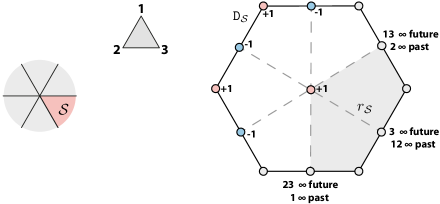
Figure 2. A cell $\mathcal{S}$ over $\{1,2,3\}$ (on the adjoint braid arrangement) and its Dynkin element $\mathtt{D}_{\mathcal{S}}$ (on the tropical geometric realization of $\boldsymbol{\Sigma}$, where the multiplication embeds facets and the comultiplication projects onto facets, see [NO19, Introduction])). In the presence of causal factorization, the time component of the corresponding generalized retarded function $r_{\mathcal{S}}$ is a $\mathbb{C}[[\hbar,\emph{{g}}]]$-valued generalized function on the braid arrangement with support the gray cone. The Dynkin element shown is $\mathtt{D}_{\mathcal{S}}=\mathtt{D}_{3}=\mathtt{R}_{(12;3)}$. Its support consists of those configurations such that the event labeled by $3$ can be causally influenced by the events labeled by $1$ and $2$.

Let

$$[I;\text{2}]:=\big{\{}\text{surjective functions}\ I\to\{1,2\}\big{\}}$$

denote the set of compositions of $I$ with two lumps. Recall that the set of minuscule weights of (the root datum of) $\text{SL}_{I}(\mathbb{C})$ is in natural bijection with $[I;\text{2}]$. We denote the minuscule weight corresponding to $(S,T)$ by $\lambda_{ST}$. See [NO19, Section 3.1] for more details.

A cell [EGS75, Definition 6] over $I$ is (equivalent to) a subset $\mathcal{S}\subseteq[I;\text{2}]$ such that for all $(S,T)\in[I;\text{2}]$, exactly one of

$$(S,T)\in\mathcal{S}\qquad\text{and}\qquad(T,S)\in\mathcal{S}$$

is true, and whose corresponding set of minuscule weights is closed under conical combinations, that is

$$\lambda_{UV}\in\text{coni}\big{\langle}\lambda_{ST}:(S,T)\in\mathcal{S}\big{\rangle}\quad\implies\quad(U,V)\in\mathcal{S}.$$

By dualizing conical spaces generated by minuscule weights, cells are in natural bijection with chambers of the adjoint of the braid arrangement, see [NO19, Section 3.3], [Eps16, Definition 2.5]. Their number is sequence A034997 in the OEIS. We denote the species of formal $\Bbbk$-linear combinations of cells by $\textbf{L}^{\vee}$.

Associated to each composition $F$ of $I$ is the subset $\mathcal{F}_{F}\subseteq[I;\text{2}]$ consisting of those compositions $(S,T)$ which are obtained by merging contiguous lumps of $F$,

$$\mathcal{F}_{F}:=\big{\{}(S,T)\in[I;\text{2}]:(S,T)\leq F\big{\}}.$$

More geometrically, $\mathcal{F}_{F}$ is the subset corresponding to the set of minuscule weights which are contained in the closed braid arrangement face of $F$. Let us write $F\subseteq\mathcal{S}$ to indicate that $\mathcal{F}_{F}\subseteq\mathcal{S}$.

Consider the morphism of species given by

(38) $$\textbf{L}^{\vee}\to\boldsymbol{\Sigma},\qquad\mathcal{S}\mapsto\mathtt{D}_{\mathcal{S}}:=-\sum_{\bar{F}\subseteq\mathcal{S}}(-1)^{l(F)}\mathtt{H}_{F}.$$

The element $\mathtt{D}_{\mathcal{S}}$ is called the Dynkin element associated to the cell $\mathcal{S}$. These special elements were defined by Epstein-Glaser-Stora in [EGS75, Equation 1, p.26], and the name is due to Aguiar-Mahajan [AM17, Equation 14.1] (see 7.1). In fact, $\mathtt{D}_{\mathcal{S}}$ is a primitive element [AM17, Proposition 14.1], and so we actually have a morphism $\textbf{L}^{\vee}\to\textbf{Zie}$.

For $i\in I$, let $\mathcal{S}_{i}$ denote the cell given by

$$\mathcal{S}_{i}:=\big{\{}(S,T)\in[I,\text{2}]:i\in S\big{\}}.$$

This is the cell corresponding to the adjoint braid arrangement chamber which contains the projection of the basis element $e_{i}\in\mathbb{R}I$ onto the sum-zero hyperplane. Let the total retarded Dynkin element $\mathtt{D}_{i}$ associated to $i$ be given by

$$\mathtt{D}_{i}:=\mathtt{D}_{\mathcal{S}_{i}}=-\sum_{\begin{subarray}{c}F\in\Sigma[I]\\ i\in S_{k}\end{subarray}}(-1)^{l(F)}\mathtt{H}_{F}.$$

These Dynkin elements are considered in [AM13, Section 14.5]. For $i\in I$, let

$$\bar{\mathcal{S}}_{i}:=\big{\{}(S,T)\in[I,\text{2}]:i\in T\big{\}}.$$

This is the cell corresponding to the adjoint braid arrangement chamber which is opposite to the chamber of $\mathcal{S}_{i}$. Let the total advanced Dynkin element $\mathtt{D}_{\bar{i}}$ associated to $i$ be given by

$$\mathtt{D}_{\bar{i}}:=\mathtt{D}_{\bar{\mathcal{S}}_{i}}=-\sum_{\begin{subarray}{c}F\in\Sigma[I]\\ i\in S_{1}\end{subarray}}(-1)^{l(F)}\mathtt{H}_{F}.$$

Remark 7.1.

More generally, Dynkin elements are certain Zie elements of generic real hyperplane arrangements, which are indexed by chambers of the corresponding adjoint arrangement. They were introduced by Aguiar-Mahajan in [AM17, Equation 14.1]. Specializing to the braid arrangement, one recovers the type $A$ Dynkin elements $\mathtt{D}_{\mathcal{S}}$.

In [NO19], the following perspective on the Dynkin elements is given. The Hopf algebra $\boldsymbol{\Sigma}^{\ast}$ which is dual to $\boldsymbol{\Sigma}$ is realized as an algebra $\hat{\boldsymbol{\Sigma}}^{\ast}$ of piecewise-constant functions on the braid arrangement. Then its dual, in the sense of polyhedral algebras [BP99, Theorem 2.7], is an algebra $\check{\boldsymbol{\Sigma}}^{\ast}$ of certain functionals of piecewise-constant functions on the adjoint braid arrangement, i.e. those coming from evaluating on permutohedral cones. We have the morphism of species

$$\check{\boldsymbol{\Sigma}}^{\ast}\to\mathcal{H}(\textbf{L}^{\vee},\textbf{E})$$

defined by sending functionals to their restrictions to piecewise-constant functions on the complement of the hyperplanes. Since the multiplication of $\check{\boldsymbol{\Sigma}}^{\ast}$ corresponds to embedding hyperplanes, this morphism is the indecomposable quotient of $\check{\boldsymbol{\Sigma}}^{\ast}$ [NO19, Theorem 4.5]. Then, in [NO19, Proposition 5.1], we see that taking the linear dual of this morphism recovers the Dynkin elements map,

$$\textbf{L}^{\vee}\to\boldsymbol{\Sigma},\qquad\mathcal{S}\mapsto\mathtt{D}_{\mathcal{S}}.$$

(Here we have identified $\boldsymbol{\Sigma}^{\ast}=\check{\boldsymbol{\Sigma}}^{\ast}$.) Therefore we obtain the following.

Theorem 7.1 ([NO19]).

The morphism of species $\textbf{L}^{\vee}\to\textbf{Zie}$ is surjective. Therefore the Dynkin elements $\{\mathtt{D}_{\mathcal{S}}:\mathcal{S}\ \text{is a cell over $I$}\}$ span Zie.

7.6. The Steinmann Relations

The Dynkin elements are not linearly independent. The relations which are satisfied by the Dynkin elements are generated by relations known in physics as the Steinmann relations, introduced in [Ste60a], [Ste60b].

Let a pair of overlapping channels over $I$ be a pair $(S,T),(U,V)\in[I;\text{2}]$ of two-lump compositions of $I$ such that

$$S\cap U\neq\emptyset\qquad\text{and}\qquad T\cap U\neq\emptyset.$$

Let $\mathcal{S}_{1}$, $\mathcal{S}_{2}$, $\mathcal{S}_{3}$, $\mathcal{S}_{4}$ be four cells over $I$ with $(S,T),(U,V)\in\mathcal{S}_{1}$, and such that $\mathcal{S}_{2}$, $\mathcal{S}_{3}$, $\mathcal{S}_{4}$ are obtained from $\mathcal{S}_{1}$ by replacing, respectively,

$$(S,T),(U,V)\mapsto(T,S),(U,V)$$

$$(S,T),(U,V)\mapsto(T,S),(V,U)$$

$$(S,T),(U,V)\mapsto(S,T),(V,U).$$

Then, by inspecting the definition of the Dynkin elements (38), we see that

$$\underbrace{\mathtt{D}_{\mathcal{S}_{1}}-\mathtt{D}_{\mathcal{S}_{2}}+\mathtt{D}_{\mathcal{S}_{3}}-\mathtt{D}_{\mathcal{S}_{4}}=0.}_{\text{Steinmann relation}}$$

In general, a Steinmann relation is any relation between Dynkin elements obtained in this way, i.e. an alternating sum of four Dynkin elements which are obtained from each other by switching overlapping channels only. This definition of the Steinmann relations can be found in [EGS75, Seciton 4.3] (it is given slightly more generally there for paracells).

An alternative characterization of the Steinmann relations in terms of the Lie cobracket of the dual Lie coalgebra $\textbf{Zie}^{\ast}$ is [LNO19, Definition 4.2]. Here, the Steinmann relations appear in the same way one can arrive at generalized permutohedra, i.e. by insisting on type $A$ ‘factorization’ in the sense of species-theoretic coalgebra structure. See [NO19, Theorem 4.2 and Remark 4.2].

So, the Dynkin elements satisfy the Steinmann relations. Moreover, we have the following.

Theorem 7.2.

The relations which are satisfied by the Dynkin elements are generated by the Steinmann relations. That is, if

$$\textbf{Stein}[I]:=\big{\langle}\mathtt{D}_{\mathcal{S}_{1}}-\mathtt{D}_{\mathcal{S}_{2}}+\mathtt{D}_{\mathcal{S}_{3}}-\mathtt{D}_{\mathcal{S}_{4}}:\mathtt{D}_{\mathcal{S}_{1}}-\mathtt{D}_{\mathcal{S}_{2}}+\mathtt{D}_{\mathcal{S}_{3}}-\mathtt{D}_{\mathcal{S}_{4}}=0\text{ is a Steinmann relation}\big{\rangle}$$

then

$$\textbf{Zie}\cong{\raisebox{1.99997pt}{$\textbf{L}^{\vee}$}\left/\raisebox{-1.99997pt}{$\textbf{Stein}$}\right.}.$$

Proof.

This follows by combining [LNO19, Theorem 4.3] with [NO19, Theorems 4.2 and 4.5]. ∎

Example 7.1.

Let us give the basic $4$-point example $I=\{1,2,3,4\}$, which takes place on a square facet of the type $A$ coroot solid [LNO19, Figure 1]. Consider the following four cells over $I$ (we have marked where they differ, the names ‘$s$-channel’ and ‘$u$-channel’ are from physics and refer to Mandelstam variables),

$$\mathcal{S}_{1}=\big{\{}\underbrace{(23,14)}_{u\text{-channel}},(12,34),(1,234),(13,24),(13,24),(134,2),(3,124)\}$$

$$\mathcal{S}_{2}=\big{\{}(23,14),\underbrace{(34,12)}_{s\text{-channel}},(1,234),(13,24),(13,24),(134,2),(3,124)\big{\}}$$

$$\mathcal{S}_{3}=\big{\{}\underbrace{(14,23)}_{u\text{-channel}},(34,12),(1,234),(13,24),(13,24),(134,2),(3,124)\big{\}}$$

$$\mathcal{S}_{4}=\big{\{}(14,23),\underbrace{(12,34)}_{s\text{-channel}},(1,234),(13,24),(13,24),(134,2),(3,124)\big{\}}.$$

The $s$-channel and the $u$-channel overlap, and so we should now have

$$\mathtt{D}_{\mathcal{S}_{1}}-\mathtt{D}_{\mathcal{S}_{2}}+\mathtt{D}_{\mathcal{S}_{3}}-\mathtt{D}_{\mathcal{S}_{4}}=0.$$

To see this, let us assume throughout that $\mathtt{H}_{F}$ appears in the $\mathtt{H}$-basis expansion (38) of $\mathtt{D}_{\mathcal{S}_{1}}$, i.e. $\bar{F}\subseteq\mathcal{S}_{1}$. Then we have

($$\spadesuit \bar{F}\subseteq\mathcal{S}_{1}\setminus\{(12,34),(23,14)\}\quad\implies\quad\bar{F}\subseteq\mathcal{S}_{1},\ \mathcal{S}_{2},\ \mathcal{S}_{3},\ \mathcal{S}_{4}.$$)

If $\bar{F}\nsubseteq\mathcal{S}_{1}\setminus\{(12,34),(23,14)\}$, then either $(12,34)\in\bar{F}$ or $(23,14)\in\bar{F}$ but not both, since the channels overlap. We then have

() $$(12,34)\in\bar{F}\implies\bar{F}\subseteq\mathcal{S}_{1},\ \bar{F}\nsubseteq\mathcal{S}_{2},\ \bar{F}\nsubseteq\mathcal{S}_{3},\ \bar{F}\subseteq\mathcal{S}_{4}.$$

We also have

() $$(23,14)\in\bar{F}\implies\bar{F}\subseteq\mathcal{S}_{1},\ \bar{F}\subseteq\mathcal{S}_{2},\ \bar{F}\nsubseteq\mathcal{S}_{3},\ \bar{F}\nsubseteq\mathcal{S}_{4}.$$

Notice that in all three cases ($\spadesuit$ ‣ 7.1), (() ‣ 7.1), (() ‣ 7.1), the prefactors of $\mathtt{H}_{F}$ sum to zero in the four term alternating sum of the Steinmann relation.

Remark 7.2.

Ocneanu [Ocn18] and Early [Ear19] have studied an affine version of the Steinmann condition, in the context of higher structures and matroid subdivisions. Here, one observes that the (translated) hyperplanes of the adjoint braid arrangement for the Mandelstam variables give three subdivisions of the hypersimplex $\Delta(2,4)$ (octahedron).

See [BC19], [CGUZ19] for the closely related study of generalized Feynman diagrams in generalized biadjoint $\Phi^{3}$-theory.

7.7. The Tits Algebra

The Hopf algebra $\boldsymbol{\Sigma}$ is also a monoid for the Hadamard product, called the Tits algebra (also called the (opposite of the) algebra of proper sequences in [EGS75]), given by

$$\boldsymbol{\Sigma}\otimes\boldsymbol{\Sigma}\to\boldsymbol{\Sigma},\qquad\mathtt{H}_{F}\otimes\mathtt{H}_{G}\mapsto\mathtt{H}_{F}\triangleright\mathtt{H}_{G}:=\mu_{F}\big{(}\Delta_{F}(\mathtt{H}_{G})\big{)}.$$

Explicitly, given compositions $F=(S_{1},\dots,S_{k_{F}})$ and $G=(T_{1},\dots,T_{k_{G}})$ of $I$, we have

$$\mu_{F}\big{(}\Delta_{F}(\mathtt{H}_{G})\big{)}=\mathtt{H}_{(T_{1}\cap S_{1},\dots,T_{k_{G}}\cap S_{1},\dots\dots,T_{1}\cap S_{k_{F}},\dots,T_{k_{G}}\cap S_{k_{F}})_{+}}.$$

The product $\mathtt{H}_{F}\triangleright\mathtt{H}_{G}$ is called the Tits product, going back to Tits [Tit74]. Its unit is $\mathtt{H}_{(I)}$. See [AM13, Section 13] for more on the structure of the Tits product. See also [AB08, Section 1.4.6] for the context of other Coxeter systems and Dynkin types.

Let us recall [AM13, Theorem 82 and Proposition 88], which describe the special role of $\boldsymbol{\Sigma}$. If h is a connected cocommutative Hopf algebra, then we have the (Tits algebra) $\boldsymbol{\Sigma}$-module $\textbf{h}=(\textbf{h},\Psi)$ where the action is taking Hopf powers,

$$\Psi:\boldsymbol{\Sigma}\otimes\textbf{h}\to\textbf{h},\qquad\mathtt{H}_{F}\otimes\mathtt{h}\mapsto\mathtt{H}_{F}\triangleright\mathtt{h}:=\mu_{F}(\Delta_{F}(\mathtt{h})).$$

The curried action

$$\widehat{\Psi}:\boldsymbol{\Sigma}\to\mathcal{E}(\textbf{h})$$

is a homomorphism of monoids for the Hadamard product. It is also a homomorphism of algebras (i.e. monoids for the Cauchy product), where $\mathcal{E}(\textbf{h})$ is equipped with the convolution algebra structure (3). In fact, if h is finite-dimensional, then $\mathcal{E}(\textbf{h})$ is naturally a Hopf algebra, and $\widehat{\Psi}$ is a homomorphism of Hopf algebras.

Proposition 7.3 ([EGS75, Lemma 8]).

Given a cell $\mathcal{S}=\big{\{}(S_{1},T_{1}),\dots,(S_{k},T_{k})\big{\}}$ over $I$, we have

$$\mathtt{D}_{\mathcal{S}}=\underbrace{(\mathtt{H}_{(I)}-\mathtt{H}_{(T_{1},S_{1})})\triangleright\,\cdots\,\triangleright(\mathtt{H}_{(I)}-\mathtt{H}_{(T_{k},S_{k})})}_{\text{these elements commute in the Tits product}}.$$

Proposition 7.4 ([EGS75, Theorem 7]).

Let $\mathcal{S}$ be a cell over $I$. Then for all $(S,T)\in\mathcal{S}$, we have

$$\mathtt{D}_{\mathcal{S}}\triangleright\mathtt{H}_{(T,S)}=0.$$

7.8. Ruelle’s Identity and the GLZ Relation

Since the Dynkin elements span Zie, we can ask what is the description of the Lie bracket of Zie in terms of the Dynkin elements. The answer is known in the physics literature as Ruelle’s identity.

In order to state Ruelle’s identity, we need to notice the following. For $S\sqcup T=I$, if $\mathcal{S}_{1}$ is a cell over $S$ and $\mathcal{S}_{2}$ is a cell over $T$, then $\mathcal{S}_{1}\sqcup\mathcal{S}_{2}$ describes a collection of codimension one faces of the adjoint braid arrangement which are supported by the hyperplane orthogonal to $\lambda_{ST}$ (in [LNO19], such faces were called Steinmann equivalent). A cell $\mathcal{S}^{[S,T]}$ over $I$ which satisfies

$$\mathcal{S}^{[S,T]}\supseteq\mathcal{S}_{1}\sqcup\mathcal{S}_{2}\qquad\text{and}\qquad(S,T)\in\mathcal{S}^{[S,T]}$$

corresponds to a chamber arrived at by moving (by an arbitrarily small amount) from an interior point of a face of $\mathcal{S}_{1}\sqcup\mathcal{S}_{2}$ in the $\lambda_{ST}$ direction. In particular, such cells always exist, but they are not unique (the Steinmann relations exactly quotient out this ambiguity). The chamber obtained by moving in the opposite direction corresponds to the cell obtained by replacing $(S,T)$ with $(T,S)$ in $\mathcal{S}^{[S,T]}$.

Proposition 7.5 (Ruelle’s Identity [Rue61, Equation 6.6]).

For $S\sqcup T=I$, let $\mathcal{S}_{1}$ be a cell over $S$ and let $\mathcal{S}_{2}$ be a cell over $T$. Let $\mathcal{S}^{[S,T]}$ be a cell over $I$ which satisfies

$$\mathcal{S}^{[S,T]}\supseteq\mathcal{S}_{1}\sqcup\mathcal{S}_{2}\qquad\text{and}\qquad(S,T)\in\mathcal{S}^{[S,T]}.$$

Let $\mathcal{S}^{[T,S]}$ denote the cell obtained by replacing $(S,T)$ with $(T,S)$ in $\mathcal{S}^{[S,T]}$. Then the Lie bracket of Zie is given by

(39) $$[\mathtt{D}_{\mathcal{S}_{1}},\mathtt{D}_{\mathcal{S}_{2}}]=\mathtt{D}_{\mathcal{S}^{[S,T]}}-\mathtt{D}_{\mathcal{S}^{[T,S]}}.$$

Proof.

This result is clear from [LNO19, Section 5.2]; the Lie bracket which was given to the adjoint braid arrangement realization of Zie (denoted there by $\boldsymbol{\Gamma}$) coincides with (39). Alternatively, we can just explicitly check, as in [EGS75, Section 4.3]. ∎

If a system of interacting generalized time-ordered products is constructed as in [Ste71], [DF04], [Düt19] via total retarded products, then one includes the GLZ relation [GLZ57, Equation 11], [Düt19, Proposition 1.10.1], which is a consequence of the following relation satisfied by the Dynkin elements $\mathtt{D}_{i}=\mathtt{R}_{(X;i)}$,

$$\mathtt{D}_{i_{1}}-\mathtt{D}_{i_{2}}=\sum_{\begin{subarray}{c}(S,T)\in[\text{2};I]\\[1.0pt] i_{1}\in S,\ i_{2}\in T\end{subarray}}[\mathtt{D}_{i_{1}},\mathtt{D}_{i_{2}}]_{S,T}.$$

8. $\boldsymbol{\Sigma}$ as a Hopf E-Algebra

We now recall the Steinmann arrows, which are (or we interpret as) actions of E on $\boldsymbol{\Sigma}$. We show that they give $\boldsymbol{\Sigma}$ the structure of a Hopf E-algebra (=Hopf monoid internal to E-modules) in two ways, and thus the primitive part $\textbf{Zie}=\mathcal{P}(\boldsymbol{\Sigma})$ the structure of a Lie E-algebra in two ways.

8.1. Derivations and Coderivations of $\boldsymbol{\Sigma}$

Recall the definition of (not necessarily commutative) up (co)derivations from Section 5, or see [AM10, Section 8.12.4]. In particular, an up derivation $u$ of $\boldsymbol{\Sigma}$ is a morphism of species

$$u:\boldsymbol{\Sigma}\to\boldsymbol{\Sigma}^{\prime},\qquad\mathtt{H}_{F}\mapsto u(\mathtt{H}_{F})\qquad\quad\text{such that}\qquad u(\mathtt{H}_{F}\mathtt{H}_{G})=u(\mathtt{H}_{F})\mathtt{H}_{G}+\mathtt{H}_{F}u(\mathtt{H}_{G}).$$

An up derivation of $\boldsymbol{\Sigma}$ is determined by its values on the elements $\mathtt{H}_{(I)}$, $I\in\textsf{S}$, since then

$$u(\mathtt{H}_{F})=u(\mathtt{H}_{(S_{1})})\mathtt{H}_{(S_{2})}\dots\mathtt{H}_{(S_{k})}+\ \,\cdots\ \,+\mathtt{H}_{(S_{1})}\dots\mathtt{H}_{(S_{k-1})}u(\mathtt{H}_{(S_{k})}).$$

An up derivation must have $u(\mathtt{H}_{\emptyset})=0$, since $\mathtt{1}_{\boldsymbol{\Sigma}}=\mathtt{H}_{\emptyset}$. An up coderivation $u$ of $\boldsymbol{\Sigma}$ is a morphism of species

$$u:\boldsymbol{\Sigma}\to\boldsymbol{\Sigma}^{\prime},\qquad\mathtt{H}_{F}\mapsto u(\mathtt{H}_{F})\qquad\quad\text{such that}\qquad\Delta_{\ast S,T}\big{(}u(\mathtt{H}_{F})\big{)}=u(\mathtt{H}_{F|_{S}})\otimes\mathtt{H}_{F|_{T}}.$$

In particular, an up coderivation must have

$$\Delta_{\ast S,T}\big{(}u(\mathtt{H}_{(I)})\big{)}=u(\mathtt{H}_{(S)})\otimes\mathtt{H}_{(T)}.$$

Therefore, a biderivation $u$ of $\boldsymbol{\Sigma}$ must have

$$u(\mathtt{H}_{(i)})=a_{1}\mathtt{H}_{(\ast,i)}+a_{2}\mathtt{H}_{(\ast i)}+a_{3}\mathtt{H}_{(i,\ast)}\qquad\quad\text{where}\qquad a_{1}+a_{2}+a_{3}=0\in\Bbbk.$$

Motivated by this, given $a,b\in\Bbbk$, we define an up derivation $u_{a,b}$ of $\boldsymbol{\Sigma}$ by

(40) $$u_{a,b}:\boldsymbol{\Sigma}\to\boldsymbol{\Sigma}^{\prime},\qquad u_{a,b}(\mathtt{H}_{(I)}):=-a\mathtt{H}_{(\ast,I)}+(a+b)\mathtt{H}_{(\ast I)}-b\mathtt{H}_{(I,\ast)}.$$

Towards an explicit description, consider the following example for $I=\{1,2,3\}$,

$$u_{a,b}(\mathtt{H}_{(12,3)}) =\,u_{a,b}(\mathtt{H}_{(12)})\mathtt{H}_{(3)}+\mathtt{H}_{(12)}u_{a,b}(\mathtt{H}_{(3)})$$

$$=(-a\mathtt{H}_{(\ast,12)}+(a+b)\mathtt{H}_{(\ast 12)}-b\mathtt{H}_{(12,\ast)})\mathtt{H}_{(3)}+\mathtt{H}_{(12)}(-a\mathtt{H}_{(\ast,3)}+(a+b)\mathtt{H}_{(\ast 3)}-b\mathtt{H}_{(3,\ast)})$$

$$=-a\mathtt{H}_{(\ast,12,3)}+(a+b)\mathtt{H}_{(\ast 12,3)}-b\mathtt{H}_{(12,\ast,3)})-a\mathtt{H}_{(12,\ast,3)}+(a+b)\mathtt{H}_{(12,\ast 3)}-b\mathtt{H}_{(12,3,\ast)}.$$

From this, we see that in general

$$u_{a,b}(\mathtt{H}_{F})=\sum_{1\leq m\leq k}-a\mathtt{H}_{(S_{1},\dots,\ast,S_{m},\dots,S_{k})}+(a+b)\mathtt{H}_{(S_{1},\dots,\ast S_{m},\dots,S_{k})}-b\mathtt{H}_{(S_{1},\dots,S_{m},\ast,\dots,S_{k})}.$$

Theorem 8.1.

Given $a,b\in\Bbbk$, the up operator

$$\boldsymbol{\Sigma}\to\boldsymbol{\Sigma}^{\prime},\qquad\mathtt{H}_{F}\mapsto u_{a,b}(\mathtt{H}_{F})$$

is a biderivation of $\boldsymbol{\Sigma}$ (and so gives $\boldsymbol{\Sigma}$ the structure of a Hopf L-algebra).

Proof.

In the following, for $F=(S_{1},\dots,S_{k})$ a composition of $I$ and $S\subseteq I$, we write

$$(U_{1},\dots,U_{k}):=(S_{1}\cap S,\dots,S_{k}\cap S).$$

In general, $(U_{1},\dots,U_{k})$ is a decomposition of $I$.

First, $u_{a,b}$ defines a derivation of $\boldsymbol{\Sigma}$ by construction. To see that $u_{a,b}$ also defines a coderivation, we have

$$\Delta_{\ast S,T}\big{(}u_{a,b}(\mathtt{H}_{F})\big{)}\ =\ \ \ \ \ \Delta_{\ast S,T}\Bigg{(}\sum_{1\leq m\leq k}-a\mathtt{H}_{(S_{1},\dots,\ast,S_{m},\dots,S_{k})}+(a+b)\mathtt{H}_{(S_{1},\dots,\ast S_{m},\dots,S_{k})}-b\mathtt{H}_{(S_{1},\dots,S_{m},\ast,\dots,S_{k})}\Bigg{)}$$

$$=\ \ \ \ \ \Bigg{(}\sum_{1\leq m\leq k}-a\mathtt{H}_{(U_{1},\dots,\ast,U_{m},\dots,U_{k})_{+}}+(a+b)\mathtt{H}_{(U_{1},\dots,\ast U_{m},\dots,U_{k})_{+}}-b\mathtt{H}_{(U_{1},\dots,U_{m},\ast,\dots,U_{k})_{+}}\Bigg{)}\otimes\mathtt{H}_{F|_{T}}$$

$$=\ \ \ \ \ \Bigg{(}\sum_{\begin{subarray}{c}1\leq m\leq k\\[2.0pt] U_{m}\neq\emptyset\end{subarray}}-a\mathtt{H}_{(U_{1},\dots,\ast,U_{m},\dots,U_{k})_{+}}+(a+b)\mathtt{H}_{(U_{1},\dots,\ast U_{m},\dots,U_{k})_{+}}-b\mathtt{H}_{(U_{1},\dots,U_{m},\ast,\dots,U_{k})_{+}}\Bigg{)}\otimes\mathtt{H}_{F|_{T}}$$

$$+\ \underbrace{\Bigg{(}\sum_{\begin{subarray}{c}1\leq m\leq k\\[2.0pt] U_{m}=\emptyset\end{subarray}}\big{(}-a+(a+b)-b\big{)}\,\mathtt{H}_{(U_{1},\dots,U_{m-1},\ast,U_{m+1},\dots,U_{k})_{+}}\Bigg{)}}_{=0}\otimes\,\mathtt{H}_{F|_{T}}$$

$$=\ \ \ \ \ u(\mathtt{H}_{F|_{S}})\otimes\mathtt{H}_{F|_{T}}.$$

Therefore $u_{a,b}$ is a biderivation of $\boldsymbol{\Sigma}$. ∎

8.2. The Steinmann Arrows

We now recall the Steinmann arrows for $\boldsymbol{\Sigma}$, whose precise definition is due to Epstein-Glaser-Stora [EGS75, p.82-83]. The Steinmann arrows were first considered by Steinmann in settings where $\boldsymbol{\Sigma}$ is represented as operator-valued distributions [Ste60b, Section 3].

Let the retarded Steinmann arrow be the up biderivation of $\boldsymbol{\Sigma}$ given by

(41) $$\ast\downarrow(-):\boldsymbol{\Sigma}\to\boldsymbol{\Sigma}^{\prime},\qquad\ast\downarrow\mathtt{H}_{F}:=u_{1,0}(\mathtt{H}_{F})=\sum_{1\leq m\leq k}-\mathtt{H}_{(S_{1},\dots,\ast,S_{m},\dots,S_{k})}+\mathtt{H}_{(S_{1},\dots,\ast S_{m},\dots,S_{k})}.$$

Let the advanced Steinmann arrow be the up biderivation of $\boldsymbol{\Sigma}$ given by

(42) $$\ast\uparrow(-):\boldsymbol{\Sigma}\to\boldsymbol{\Sigma}^{\prime},\qquad\ast\uparrow\mathtt{H}_{F}:=u_{0,1}(\mathtt{H}_{F})=\sum_{1\leq m\leq k}\mathtt{H}_{(S_{1},\dots,\ast S_{m},\dots,S_{k})}-\mathtt{H}_{(S_{1},\dots,S_{m},\ast,\dots,S_{k})}.$$

In particular

$$\ast\downarrow\mathtt{H}_{(I)}=-\mathtt{H}_{(\ast,I)}+\mathtt{H}_{(\ast I)}\qquad\text{and}\qquad\ast\uparrow\mathtt{H}_{(I)}=\mathtt{H}_{(\ast I)}-\mathtt{H}_{(I,\ast)}.$$

We have

$$\ast\uparrow\mathtt{H}_{F}\,-\,\ast\downarrow\mathtt{H}_{F}=u_{-1,1}(\mathtt{H}_{F})=[\mathtt{H}_{(\ast)},\mathtt{H}_{F}].$$

This identity appears often in the physics literature for operator-valued distributions, e.g. [Ste60b, Equation 13], [EG73, Equation 83]. The biderivation $u_{-1,1}$ gives $\boldsymbol{\Sigma}$ the structure of a Hopf L-algebra. This L-action is the restriction of the adjoint representation of $\boldsymbol{\Sigma}$.

Notice that the Steinmann arrows are commutative up operators. Therefore, by 5.4, we can restrict them to obtain commutative up derivations of Zie,

$$\ast\downarrow(-):\textbf{Zie}\to\textbf{Zie}^{\prime},\qquad\mathtt{D}_{\mathcal{S}}\mapsto\ast\downarrow\mathtt{D}_{\mathcal{S}}\qquad\text{and}\qquad\ast\uparrow(-):\textbf{Zie}\to\textbf{Zie}^{\prime},\qquad\mathtt{D}_{\mathcal{S}}\mapsto\ast\uparrow\mathtt{D}_{\mathcal{S}}.$$

By 8.1, the Steinmann arrows equip $\boldsymbol{\Sigma}$ with the structure of a Hopf E-algebra (and Zie with the structure of a Lie E-algebra) in two ways. We denote the corresponding E-modules, as defined in (23), by

$$\textbf{E}\mathchoice{\mathbin{\vbox{\hbox{{$\displaystyle\bullet$}}}}}{\mathbin{\vbox{\hbox{{$\textstyle\bullet$}}}}}{\mathbin{\vbox{\hbox{{$\scriptstyle\bullet$}}}}}{\mathbin{\vbox{\hbox{{$\scriptscriptstyle\bullet$}}}}}\boldsymbol{\Sigma}\to\boldsymbol{\Sigma},\qquad\mathtt{H}_{Y}\otimes\mathtt{a}\mapsto Y\!\downarrow\mathtt{a}=\underbrace{y_{r}\downarrow\circ\cdots\circ y_{1}\downarrow}_{\text{invariant of the order}}(\mathtt{a})$$

and

$$\textbf{E}\mathchoice{\mathbin{\vbox{\hbox{{$\displaystyle\bullet$}}}}}{\mathbin{\vbox{\hbox{{$\textstyle\bullet$}}}}}{\mathbin{\vbox{\hbox{{$\scriptstyle\bullet$}}}}}{\mathbin{\vbox{\hbox{{$\scriptscriptstyle\bullet$}}}}}\boldsymbol{\Sigma}\to\boldsymbol{\Sigma},\qquad\mathtt{H}_{Y}\otimes\mathtt{a}\mapsto Y\!\uparrow\mathtt{a}=\underbrace{y_{r}\uparrow\circ\cdots\circ y_{1}\uparrow}_{\text{invariant of the order}}(\mathtt{a})$$

where $Y=\{y_{1},\dots,y_{r}\}$. For $Y=[r]:=\{\ast_{1},\dots,\ast_{r}\}$, we abbreviate

$$\downarrow(-):=\ast\downarrow(-),\qquad\downarrow\downarrow(-):=\{\ast_{1},\ast_{2}\}\downarrow(-),\qquad\dots$$

and similarly for the advanced arrow.

By inspecting the definitions, we see that

(43) $$Y\!\downarrow\mathtt{H}_{(I)}=\mathtt{R}_{(Y;I)}:=\!\sum_{Y_{1}\sqcup Y_{2}=Y}\overline{\mathtt{H}}_{(Y_{1})}\mathtt{H}_{(Y_{2}\sqcup I)}\qquad\text{and}\qquad Y\!\uparrow\mathtt{H}_{(I)}=\mathtt{A}_{(Y;I)}:=\!\sum_{Y_{1}\sqcup Y_{2}=Y}\mathtt{H}_{(Y_{1}\sqcup I)}\overline{\mathtt{H}}_{(Y_{2})}.$$

It follows that

$$Y\!\downarrow\mathtt{H}_{F}=\sum_{Y_{1}\sqcup\dots\sqcup Y_{k}=Y}\mathtt{R}_{(Y_{1};S_{1})}\dots\mathtt{R}_{(Y_{k};S_{k})}\qquad\text{and}\qquad Y\!\uparrow\mathtt{H}_{F}=\sum_{Y_{1}\sqcup\dots\sqcup Y_{k}=Y}\mathtt{A}_{(Y_{1};S_{1})}\dots\mathtt{A}_{(Y_{k};S_{k})}.$$

The sums are over all decompositions $(Y_{1},\dots,Y_{k})$ of $Y$ of length $l(F)$. We call $\mathtt{R}_{(Y;I)},\mathtt{A}_{(Y;I)}\in\boldsymbol{\Sigma}[Y\sqcup I]$ the retarded and advanced elements respectively. The total retarded and total advanced elements are given by

$$Y\!\downarrow\mathtt{H}_{(i)}=\mathtt{R}_{(Y;i)}=\sum_{Y_{1}\sqcup Y_{2}=Y}\overline{\mathtt{H}}_{(Y_{1})}\,\mathtt{H}_{(Y_{2}i)}\qquad\text{and}\qquad Y\!\uparrow\mathtt{H}_{(i)}=\mathtt{A}_{(Y;i)}=\sum_{Y_{1}\sqcup Y_{2}=Y}\mathtt{H}_{(Y_{2}i)}\,\overline{\mathtt{H}}_{(Y_{1})}$$

respectively.

Remark 8.1.

If we put $I=X\sqcup\{i\}$, then we have

$$\mathtt{R}_{(X;i)}=\sum_{\begin{subarray}{c}S\sqcup T=I\\ i\in T\end{subarray}}\overline{\mathtt{H}}_{(S)}\,\mathtt{H}_{(T)}=-\sum_{\begin{subarray}{c}F\in\Sigma[I]\\ i\in S_{k}\end{subarray}}(-1)^{l(F)}\mathtt{H}_{F}=\mathtt{D}_{i}$$

and

$$\mathtt{A}_{(X;i)}=\sum_{\begin{subarray}{c}S\sqcup T=I\\ i\in T\end{subarray}}\mathtt{H}_{(T)}\,\overline{\mathtt{H}}_{(S)}=-\sum_{\begin{subarray}{c}F\in\Sigma[I]\\ i\in S_{1}\end{subarray}}(-1)^{l(F)}\mathtt{H}_{F}=\mathtt{D}_{\bar{i}}.$$

Theorem 8.2.

We have the following homomorphisms of algebras in species,

$$\boldsymbol{\Sigma}\to\boldsymbol{\Sigma}^{\textbf{E}},\qquad\mathtt{H}_{F}\mapsto\sum_{Y_{1}\sqcup\dots\sqcup Y_{k}=(-)}\mathtt{R}_{(Y_{1};S_{1})}\dots\mathtt{R}_{(Y_{k};S_{k})}=\sum_{r=0}^{\infty}\,\sum_{Y_{1}\sqcup\dots\sqcup Y_{k}=[r]}\mathtt{R}_{(Y_{1};S_{1})}\dots\mathtt{R}_{(Y_{k};S_{k})}$$

and

$$\boldsymbol{\Sigma}\to\boldsymbol{\Sigma}^{\textbf{E}},\qquad\mathtt{H}_{F}\mapsto\sum_{Y_{1}\sqcup\dots\sqcup Y_{k}=(-)}\mathtt{A}_{(Y_{1};S_{1})}\dots\mathtt{A}_{(Y_{k};S_{k})}=\sum_{r=0}^{\infty}\,\sum_{Y_{1}\sqcup\dots\sqcup Y_{k}=[r]}\mathtt{A}_{(Y_{1};S_{1})}\dots\mathtt{A}_{(Y_{k};S_{k})}.$$

Proof.

The Steinmann arrows are commutative up biderivations of $\boldsymbol{\Sigma}$, and so give $\boldsymbol{\Sigma}$ the structure of a Hopf E-algebra. The maps here are the associated $(-)^{\textbf{E}}$-coalgebras obtained by currying the actions of E, which are homomorphisms by 5.1. ∎

The homomorphisms of 8.2 are the unique extensions of the maps

$$\mathtt{H}_{(I)}\mapsto\sum_{r=0}^{\infty}\mathtt{R}_{(r;I)}\qquad\text{and}\qquad\mathtt{H}_{(I)}\mapsto\sum_{r=0}^{\infty}\mathtt{A}_{(r;I)}$$

to homomorphisms.

8.3. The Steinmann Arrows and Dynkin Elements

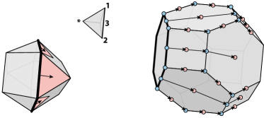
Figure 3. Schematic for the action of the retarded Steinmann arrow $\ast\downarrow$ for $I=\{1,2,3\}$ on the Steinmann sphere (left) and the tropical geometric realization of $\boldsymbol{\Sigma}$ (right, see [NO19, Introduction]).

We now show that the restriction of the Steinmann arrows to Zie, which are derivations for its Lie bracket, have an interesting description in terms of cells, i.e. chambers of the adjoint braid arrangement.

Following [Eps16, Section 2], we define the commutative up operators

$$\ast\downarrow(-):\textbf{L}^{\vee}\to{\textbf{L}^{\vee}}^{\prime},\qquad\ast\downarrow\mathcal{S}:=\big{\{}(\ast S,T),(S,\ast T),(I,\ast):(S,T)\in\mathcal{S}\big{\}}$$

and

$$\ast\uparrow(-):\textbf{L}^{\vee}\to{\textbf{L}^{\vee}}^{\prime},\qquad\ast\uparrow\mathcal{S}:=\big{\{}(\ast S,T),(S,\ast T),(\ast,I):(S,T)\in\mathcal{S}\big{\}}.$$

These are indeed well-defined; $\ast\downarrow\mathcal{S}$ corresponds to the adjoint braid arrangement chamber on the $I$ side of the hyperplane $\lambda_{\ast,I}=0$ which has the face of $\mathcal{S}$ as a facet, and $\ast\uparrow\mathcal{S}$ corresponds to the chamber on the $\ast$ side of the hyperplane $\lambda_{\ast,I}=0$ which has the face of $\mathcal{S}$ as a facet. See around [LNO19, Remark 2.2] for more details. Thus, it follows from 7.5 (Ruelle’s identity) that

$$[\mathtt{H}_{(\ast)},\mathtt{D}_{\mathcal{S}}]=\mathtt{D}_{\ast\uparrow\mathcal{S}}-\mathtt{D}_{\ast\downarrow\mathcal{S}}.$$

We denote the corresponding E-modules by

$$\textbf{E}\mathchoice{\mathbin{\vbox{\hbox{{$\displaystyle\bullet$}}}}}{\mathbin{\vbox{\hbox{{$\textstyle\bullet$}}}}}{\mathbin{\vbox{\hbox{{$\scriptstyle\bullet$}}}}}{\mathbin{\vbox{\hbox{{$\scriptscriptstyle\bullet$}}}}}\textbf{L}^{\vee}\to\textbf{L}^{\vee},\qquad\mathtt{H}_{Y}\otimes\mathcal{S}\mapsto Y\downarrow\mathcal{S}=\big{\{}(Y_{1}\sqcup S,Y_{2}\sqcup T)\in[Y\sqcup I;\text{2}]:(S,T)\in\mathcal{S}\ \text{or}\ S=I\big{\}}$$

and

$$\textbf{E}\mathchoice{\mathbin{\vbox{\hbox{{$\displaystyle\bullet$}}}}}{\mathbin{\vbox{\hbox{{$\textstyle\bullet$}}}}}{\mathbin{\vbox{\hbox{{$\scriptstyle\bullet$}}}}}{\mathbin{\vbox{\hbox{{$\scriptscriptstyle\bullet$}}}}}\textbf{L}^{\vee}\to\textbf{L}^{\vee},\qquad\mathtt{H}_{Y}\otimes\mathcal{S}\mapsto Y\uparrow\mathcal{S}=\big{\{}(Y_{1}\sqcup S,Y_{2}\sqcup T)\in[Y\sqcup I;\text{2}]:(S,T)\in\mathcal{S}\ \text{or}\ T=I\big{\}}.$$

Proposition 8.3.

Given a cell $\mathcal{S}$ over $I$, we have

$$Y\downarrow\mathtt{D}_{\mathcal{S}}=\mathtt{D}_{Y\downarrow\mathcal{S}}\qquad\text{and}\qquad Y\uparrow\mathtt{D}_{\mathcal{S}}=\mathtt{D}_{Y\uparrow\mathcal{S}}.$$

Proof.

We consider the retarded case $Y\downarrow\mathtt{D}_{\mathcal{S}}=\mathtt{D}_{Y\downarrow\mathcal{S}}$ only, since the advanced case then follows similarly. It is sufficient to consider the case $Y=\{\ast\}$. We have

$$\downarrow\mathtt{D}_{\mathcal{S}}=-\sum_{\bar{F}\subseteq\mathcal{S}}(-1)^{l(F)}\downarrow\mathtt{H}_{F}\qquad\text{and}\qquad\mathtt{D}_{\downarrow\mathcal{S}}=-\sum_{\bar{F}\subseteq\,\downarrow\mathcal{S}}(-1)^{l(F)}\,\mathtt{H}_{F}.$$

So, the result follows if we have the following equality

$$\sum_{\bar{F}\subseteq\mathcal{S}}(-1)^{l(F)}\sum_{1\leq m\leq k}-\mathtt{H}_{(S_{1},\dots,\ast,S_{m},\dots,S_{k})}+\mathtt{H}_{(S_{1},\dots,\ast S_{m},\dots,S_{k})}\overset{\mathrm{?}}{=}\sum_{\bar{G}\subseteq\,\downarrow\mathcal{S}}(-1)^{l(G)}\,\mathtt{H}_{G}.$$

Indeed, notice that the $\mathtt{H}$-basis elements $\mathtt{H}_{G}\in\boldsymbol{\Sigma}[\ast I]$ which appear on the LHS are exactly those such that

$$\bar{G}\subseteq\downarrow\mathcal{S}.$$

Notice also that each $\mathtt{H}_{G}$ appears with total sign $(-1)^{l(G)}$, since when $\ast$ is inserted as a singleton lump, thus increasing $l(G)$ by one, it appears also with a negative sign. ∎

Remark 8.2.

This interpretation of the E-module structure of $\boldsymbol{\Sigma}$ restricted to the primitive part $\textbf{Zie}=\mathcal{P}(\boldsymbol{\Sigma})$ in terms of the adjoint braid arrangement suggests obvious generalizations of the Steinmann arrows in the direction of [AM17], [AM20], since the generalization of Hopf monoids there is via hyperplane arrangements.

Corollary 8.3.1.

We have the following homomorphisms of Lie algebras in species,

$$\textbf{Zie}\to\textbf{Zie}^{\textbf{E}},\qquad\mathtt{D}_{\mathcal{S}}\mapsto\mathtt{D}_{(-)\downarrow\mathcal{S}}=\sum_{r=0}^{\infty}\mathtt{D}_{[r]\downarrow\mathcal{S}}=\mathtt{D}_{\mathcal{S}}+\mathtt{D}_{\downarrow\mathcal{S}}+\mathtt{D}_{\downarrow\downarrow\mathcal{S}}+\cdots$$

and

$$\textbf{Zie}\to\textbf{Zie}^{\textbf{E}},\qquad\mathtt{D}_{\mathcal{S}}\mapsto\mathtt{D}_{(-)\uparrow\mathcal{S}}=\sum_{r=0}^{\infty}\mathtt{D}_{[r]\uparrow\mathcal{S}}=\mathtt{D}_{\mathcal{S}}+\mathtt{D}_{\uparrow\mathcal{S}}+\mathtt{D}_{\uparrow\uparrow\mathcal{S}}+\cdots.$$

Proof.

The Steinmann arrows are commutative up biderivations of Zie, and so give Zie the structure of a Lie E-algebra. The maps given here are the associated $(-)^{\textbf{E}}$-coalgebras obtained by currying the actions of E, which are homomorphisms by 5.1. ∎

9. Products and Series

We now recall several basic constructions of casual perturbation theory in the current, clean, abstract setting. We do this without yet imposing causal factorization/causal additivity. We say e.g. ‘T-product’ and ‘R-product’ for now, and then change to ‘time-ordered product’ and ‘retarded product’ in the presence of causal factorization.

9.1. T-Products, Generalized T-Products, and Generalized R-Products

Let $V$ be a vector space over $\Bbbk$, and let $\mathcal{A}$ be a $\Bbbk$-algebra with multiplication denoted by $\star$. Let a system of T-products T be a system of products (as defined in Section 6.2) for the positive exponential species $\textbf{E}^{\ast}_{+}$,

$$\text{T}:\textbf{E}^{\ast}_{+}\otimes\textbf{E}_{V}\to\textbf{U}_{\mathcal{A}},\qquad\mathtt{H}_{(I)}\otimes\emph{{A}}_{I}\mapsto\text{T}_{I}(\mathtt{H}_{(I)}\otimes\emph{{A}}_{I}).$$

We abbreviate

$$\text{T}_{I}(\emph{{A}}_{I}):=\text{T}_{I}(\mathtt{H}_{(I)}\otimes\emph{{A}}_{I}).$$

The currying of T is denoted by

$$\textbf{E}^{\ast}_{+}\to\mathcal{H}(\textbf{E}_{V},\textbf{U}_{\mathcal{A}}),\qquad\mathtt{H}_{(I)}\mapsto\text{T}(I)$$

where the linear maps

$$\text{T}(I):\textbf{E}_{V}[I]\to\mathcal{A},\qquad\emph{{A}}_{I}\mapsto\text{T}_{I}(\emph{{A}}_{I})$$

are called T-products. Notice that T-products are commutative in the sense that

$$\text{T}_{I}\big{(}\textbf{E}_{V}[\sigma](\emph{{A}}_{I})\big{)}=\text{T}_{I}(\emph{{A}}_{I})\qquad\quad\text{for all bijections}\quad\sigma:I\to I.$$

This property holds because the system T is a morphism of species, and bijections act trivially for $\textbf{U}_{\mathcal{A}}$. This commutativity exists despite the fact that the algebra $\mathcal{A}$ is noncommutative in general.

Remark 9.1.

In applications to QFT, we shall also have a causal structure on $V$. Then T is meant to first order the vectors of $\emph{{A}}_{I}$ according to the causal structure, and then multiply in $\mathcal{A}$, giving rise to this commutativity.

Let the system of generalized T-products associated to a system of T-products be the unique extension to an algebraic system of products for $\boldsymbol{\Sigma}=\textbf{L}\boldsymbol{\circ}\textbf{E}_{+}^{\ast}$, thus

$$\text{T}:\boldsymbol{\Sigma}\otimes\textbf{E}_{V}\to\textbf{U}_{\mathcal{A}},\qquad\mathtt{H}_{F}\otimes\emph{{A}}_{I}\mapsto\text{T}_{I}(\mathtt{H}_{F}\otimes\emph{{A}}_{I}):=\text{T}_{S_{1}}(\emph{{A}}_{S_{1}})\star\dots\star\text{T}_{S_{k}}(\emph{{A}}_{S_{k}}).$$

The currying of T is denoted by

$$\boldsymbol{\Sigma}\to\mathcal{H}(\textbf{E}_{V},\textbf{U}_{\mathcal{A}}),\qquad\mathtt{H}_{F}\mapsto\text{T}(S_{1})\dots\text{T}(S_{k}).$$

The linear maps

$$\text{T}(S_{1})\dots\text{T}(S_{k}):\textbf{E}_{V}[I]\to\mathcal{A},\qquad\emph{{A}}_{I}\mapsto\text{T}_{I}(\mathtt{H}_{F}\otimes\emph{{A}}_{I})$$

are called generalized T-products. Let the system of generalized R-products associated to a system of T-products be the restriction to the Lie algebra of primitive elements Zie,

$$\text{R}:\textbf{Zie}\otimes\textbf{E}_{V}\to\textbf{U}_{\mathcal{A}},\qquad\mathtt{D}_{\mathcal{S}}\otimes\emph{{A}}_{I}\mapsto\text{R}_{I}(\mathtt{D}_{\mathcal{S}}\otimes\emph{{A}}_{I}):=\text{T}_{I}(\mathtt{D}_{\mathcal{S}}\otimes\emph{{A}}_{I}).$$

This is a morphism of Lie algebras, where $\textbf{U}_{\mathcal{A}}$ is equipped with the commutator bracket. The currying of R is denoted by

$$\textbf{Zie}\to\mathcal{H}(\textbf{E}_{V},\textbf{U}_{\mathcal{A}}),\qquad\mathtt{D}_{\mathcal{S}}\mapsto\text{R}_{\mathcal{S}}.$$

The linear maps

$$\text{R}_{\mathcal{S}}:\textbf{E}_{V}[I]\to\mathcal{A},\qquad\emph{{A}}_{I}\mapsto\text{R}_{I}(\mathtt{D}_{\mathcal{S}}\otimes\emph{{A}}_{I})$$

are called generalized R-products. From the expansion (38) of Dynkin elements $\mathtt{D}_{\mathcal{S}}$ in terms of the $\mathtt{H}$-basis, we recover [EG73, Equation 79],

$$\text{R}_{\mathcal{S}}=-\sum_{\mathcal{F}_{F}\subseteq\bar{\mathcal{S}}}(-1)^{k}\,\text{T}(S_{1})\dots\text{T}(S_{k}).$$

Consider a system of products of the form

$$\text{Z}:\textbf{E}^{\ast}_{+}\otimes{\textbf{E}_{V}}\to\textbf{U}_{V},\qquad\mathtt{H}_{(I)}\otimes\emph{{A}}_{I}\mapsto\text{Z}_{I}(\emph{{A}}_{I}).$$

Then we obtain a new T-product $\text{T}^{\prime}$, given by

$$\text{T}^{\prime}:\textbf{E}^{\ast}_{+}\otimes\textbf{E}_{V}\to\textbf{U}_{\mathcal{A}},\qquad\text{T}^{\prime}_{I}(\emph{{A}}_{I}):=\sum_{P}\text{T}_{P}\big{(}\text{Z}_{S_{1}}(\emph{{A}}_{S_{1}})\dots\text{Z}_{S_{k}}(\emph{{A}}_{S_{k}})\big{)}.$$

The sum is over all partitions $P=\{S_{1},\dots,S_{k}\}$ of $I$. This construction underlies renormalization in pAQFT [Düt19, Section 3.6.2], which deals with the remaining ambiguity of T-products after imposing causal factorization, and perhaps other renormalization conditions.

Remark 9.2.

We have the presheaf of compositions $\Sigma:\textsf{S}^{\text{op}}\to\textsf{Set}$, and we may pick a monoidal copresheaf $\textbf{E}_{V}:\textsf{S}\to\textsf{Vec}$. Then a system of generalized T-products is equivalently a homomorphism on the weighted colimit $\overline{\mathcal{K}}_{V}(\boldsymbol{\Sigma})=\Sigma\otimes_{\textsf{S}}\textbf{E}_{V}$ into some $\Bbbk$-algebra $\mathcal{A}$. In fact, letting $\textbf{E}_{V}$ be a copresheaf is more natural in the application to QFT.

9.2. Reverse T-Products

The system of reverse generalized T-products $\overline{\text{T}}$ of a system of generalized T-products is given by precomposing T with the antipode (37) of $\boldsymbol{\Sigma}\otimes\textbf{E}_{V}$, thus

$$\overline{\text{T}}:\boldsymbol{\Sigma}\otimes{\textbf{E}}_{V}\to\textbf{U}_{\mathcal{A}^{\operatorname{op}}},\qquad\overline{\text{T}}_{I}(\mathtt{H}_{F}\otimes\emph{{A}}_{I}):={\text{T}}_{I}\big{(}\overline{\mathtt{H}}_{F}\otimes\emph{{A}}_{I}\big{)}.$$

Since the antipode is a homomorphism $\boldsymbol{\Sigma}\otimes\textbf{E}_{V}\to(\boldsymbol{\Sigma}\otimes\textbf{E}_{V})^{\operatorname{op},\text{cop}}$ [AM10, Proposition 1.22 (iii)], this is a system of generalized T-products into the opposite algebra $\textbf{U}_{\mathcal{A}^{\operatorname{op}}}$. The image of $\mathtt{H}_{(I)}$ under the currying of $\overline{\text{T}}$ is called the reverse T-product

$$\overline{\text{T}}(I):\textbf{E}_{V}[I]\to\mathcal{A}^{\text{op}}.$$

From (35), we obtain

$$\overline{\text{T}}(I)=\sum_{F\in\Sigma[I]}(-1)^{k}\,\text{T}(S_{1})\dots\text{T}(S_{k}).$$

Note that reverse T-products in [EG73, Equation 11] are defined to be $(-1)^{n}\,\overline{\text{T}}(I)$. Our definition agrees with [Sch20, Definition 15.35].

9.3. T-Exponentials

The (scaled) universal series $\mathtt{G}(c)\in\mathscr{S}(\boldsymbol{\Sigma})$ is the group-like series of $\boldsymbol{\Sigma}$ given by

$$\mathtt{G}(c):\textbf{E}\to\boldsymbol{\Sigma},\qquad\mathtt{H}_{I}\mapsto\mathtt{G}(c)_{I}:=c^{n}\,\mathtt{H}_{(I)}\qquad\quad\text{for}\quad c\in\Bbbk.$$

The fundamental nature of this series is described in [AM13, Section 13.6]. The series $\text{s}\circ\mathtt{G}(c)$ which is the composition of $\mathtt{G}(c)$ with the antipode s of $\boldsymbol{\Sigma}$ is given by

(44) $$\text{s}\circ\mathtt{G}(c):\textbf{E}\to\boldsymbol{\Sigma},\qquad\mathtt{H}_{I}\mapsto\big{(}\text{s}\circ\mathtt{G}(c)\big{)}_{I}=c^{n}\,\overline{\mathtt{H}}_{(I)}.$$

Given a system of generalized T-products $\text{T}:\boldsymbol{\Sigma}\otimes{\textbf{E}}_{V}\to\textbf{U}_{\mathcal{A}}$, let the T-exponential $\mathcal{S}:=\mathcal{S}_{\mathtt{G}(c)}$ of this system be the $\mathcal{A}[[\emph{{j}}\,]]$-valued function on the vector space $V$ associated to the series $\mathtt{G}(c)$, as constructed in Section 6.3. Thus, we have

(45) $$\mathcal{S}:V\to\mathcal{A}[[\emph{{j}}\,]],\qquad\emph{{A}}\mapsto\mathcal{S}(\emph{{j}}\,\!\emph{{A}})=\sum^{\infty}_{n=0}\dfrac{c^{n}}{n!}\text{T}_{n}\underbrace{\big{(}\emph{{j}}\,\!\emph{{A}}\otimes\cdots\otimes\emph{{j}}\,\!\emph{{A}}\big{)}}_{\text{ $n$ times }}=\sum^{\infty}_{n=0}\dfrac{\emph{{j}}\,^{n}c^{n}}{n!}\text{T}_{n}(\emph{{A}}^{n}).$$

By (34) and (44), the T-exponential for the system of reverse T-products is the inverse of $\mathcal{S}$ as an element of the $\Bbbk$-algebra of functions $\text{Func}(V,\mathcal{A}[[\emph{{j}}\,]])$, given by

$$\mathcal{S}^{-1}:V\to\mathcal{A}[[\emph{{j}}\,]],\qquad\emph{{A}}\mapsto\mathcal{S}^{-1}(\emph{{j}}\,\!\emph{{A}}):=\sum^{\infty}_{n=0}\dfrac{\emph{{j}}\,^{n}c^{n}}{n!}\overline{\text{T}}_{n}(\emph{{A}}^{n})=\sum^{\infty}_{n=0}\dfrac{\emph{{j}}\,^{n}c^{n}}{n!}\text{T}_{n}(\overline{\mathtt{H}}_{(n)}\otimes\emph{{A}}^{n}).$$

Therefore

$$\mathcal{S}(\emph{{j}}\,\!\emph{{A}})\star\mathcal{S}^{-1}(\emph{{j}}\,\!\emph{{A}})=\mathcal{S}^{-1}(\emph{{j}}\,\!\emph{{A}})\star\mathcal{S}(\emph{{j}}\,\!\emph{{A}})=1_{\mathcal{A}}$$

for all $\emph{{A}}\in V$. This appears in e.g. [EG73, Equation 2].

10. Perturbation of T-Products

We now construct three perturbations of T-products by E-actions, as considered in Section 6.4.

10.1. Perturbation of T-Products by Up Coderivation

Suppose we have a system of T-products

$$\text{T}:\textbf{E}^{\ast}_{+}\otimes\textbf{E}_{V}\to\textbf{U}_{\mathcal{A}},\qquad\mathtt{H}_{(I)}\otimes\emph{{A}}_{I}\mapsto\text{T}_{I}(\emph{{A}}_{I}).$$

Following Section 6.4, given a choice of decorations vector $\emph{{S}}\in V$, we can use the up coderivation

$$u:\textbf{E}_{V}\to\textbf{E}^{\prime}_{V},\qquad u(\emph{{A}}_{I})=\emph{{S}}\emph{{A}}_{I}$$

from Section 6.1 to perturb T, giving

$$\textbf{E}_{+}^{\ast}\otimes\textbf{E}_{V}\to\textbf{U}_{\mathcal{A}[[\emph{{g}}]]},\quad\mathtt{H}_{(I)}\otimes\emph{{A}}_{I}\mapsto\sum_{r=0}^{\infty}\dfrac{\emph{{g}}^{\,r\,}}{r!}\text{T}^{r}_{I}(\emph{{S}}^{\,r}\emph{{A}}_{I})=\text{T}_{I}(\emph{{A}}_{I})+\underbrace{\emph{{g}}\,\text{T}^{1}_{I}(\emph{{S}}\emph{{A}}_{I})+\dfrac{\emph{{g}}^{2}}{2!}\text{T}^{2}_{I}(\emph{{S}}\emph{{S}}\emph{{A}}_{I})+\cdots}_{\text{perturbation}}\ .$$

Let $\mathcal{S}_{\emph{{g}}\emph{{S}}}$ denote the T-exponential for this new perturbed system of T-products (as defined in (45)), thus

$$\mathcal{S}_{\emph{{g}}\emph{{S}}}:V\to\mathcal{A}[[\emph{{g}},\!\emph{{j}}\,]],\qquad\emph{{A}}\mapsto\mathcal{S}_{\emph{{g}}\emph{{S}}}(\emph{{j}}\,\!\emph{{A}}):=\sum^{\infty}_{n=0}\sum_{r=0}^{\infty}\dfrac{\emph{{g}}^{r}\emph{{j}}\,^{n}\,c^{r+n}}{r!\,n!}\text{T}^{r}_{n}(\emph{{S}}^{\,r}\emph{{A}}^{n})$$

for $c\in\Bbbk$.

Proposition 10.1.

Given vectors $\emph{{S}},\emph{{A}}\in V$, we have

$$\mathcal{S}_{\emph{{g}}\emph{{S}}}(\emph{{j}}\,\!\emph{{A}})=\mathcal{S}(\emph{{g}}\emph{{S}}+\emph{{j}}\,\!\emph{{A}}).$$

Proof.

We have

$$\mathcal{S}_{\emph{{g}}\emph{{S}}}(\emph{{j}}\,\!\emph{{A}})=\sum^{\infty}_{n=0}\sum^{\infty}_{r=0}\dfrac{\emph{{g}}^{r}\emph{{j}}\,^{n}\,c^{r+n}}{r!\,n!}{\text{T}^{r}_{n}}(\emph{{S}}^{\,r}\emph{{A}}^{n})=\sum^{\infty}_{k=0}\dfrac{c^{k}}{k!}\text{T}_{k}\underbrace{(\emph{{g}}\emph{{S}}+\emph{{j}}\,\!\emph{{A}}\otimes\cdots\otimes\emph{{g}}\emph{{S}}+\emph{{j}}\,\!\emph{{A}})}_{k\text{ times}}.$$

The second equality is obtained by putting $k=n+r$. ∎

10.2. Perturbation of T-Products by Steinmann Arrows

Suppose we have a system of generalized T-products

$$\text{T}:\boldsymbol{\Sigma}\otimes\textbf{E}_{V}\to\textbf{U}_{\mathcal{A}},\qquad\mathtt{H}_{F}\otimes\emph{{A}}_{I}\mapsto\text{T}_{I}(\mathtt{H}_{F}\otimes\emph{{A}}_{I}).$$

Following Section 6.4, given a choice of decorations vector $\emph{{S}}\in V$, we can use the Steinmann arrows (41) and (42) to perturb T, giving

$${\text{T}_{\downarrow,\emph{{S}}}}:\boldsymbol{\Sigma}\otimes\textbf{E}_{V}\to\textbf{U}_{\mathcal{A}[[\emph{{g}}]]},\qquad{\text{T}_{\downarrow,\emph{{S}}}}:=\text{T}^{\textbf{E}}\circ{\widecheck{\rho}_{\downarrow,\emph{{S}}}}$$

for the retarded arrow, and

$${\text{T}_{\uparrow,\emph{{S}}}}:\boldsymbol{\Sigma}\otimes\textbf{E}_{V}\to\textbf{U}_{\mathcal{A}[[\emph{{g}}]]},\qquad{\text{T}_{\uparrow,\emph{{S}}}}:=\text{T}^{\textbf{E}}\circ\widecheck{\rho}_{\uparrow,\emph{{S}}}$$

for the advanced arrow. We sometimes denote $\widetilde{\text{T}}:=\,{\text{T}_{\downarrow,\emph{{S}}}}$. Towards an explicit description of these new perturbed systems of generalized T-products, given

$$\emph{{S}}_{Y}\emph{{A}}_{I}=\emph{{S}}_{y_{1}}\otimes\dots\otimes\emph{{S}}_{y_{r}}\otimes\emph{{A}}_{i_{1}}\otimes\dots\otimes\emph{{A}}_{i_{n}}\in\textbf{E}_{V}^{[Y]}[I],$$

let

(46) $$\text{R}_{Y;I}(\emph{{S}}_{Y};\emph{{A}}_{I}):=\underbrace{\text{T}^{[Y]}_{I}(\mathtt{R}_{(Y;I)}\otimes\emph{{S}}_{Y}\emph{{A}}_{I})=\sum_{Y_{1}\sqcup Y_{2}=Y}\overline{\text{T}}^{[Y_{1}]}_{\emptyset}(\emph{{S}}_{Y_{1}})\star\text{T}^{[Y_{2}]}_{I}(\emph{{S}}_{Y_{2}}\emph{{A}}_{I})}_{\text{by }{\color[rgb]{0,0,1}(\ref{eq:retardadvan}})}$$

and

$$\text{A}_{Y;I}(\emph{{S}}_{Y};\emph{{A}}_{I}):=\underbrace{\text{T}^{[Y]}_{I}(\mathtt{A}_{(Y;I)}\otimes\emph{{S}}_{Y}\emph{{A}}_{I})=\sum_{Y_{1}\sqcup Y_{2}=Y}\text{T}^{[Y_{1}]}_{I}(\emph{{S}}_{Y_{1}}\emph{{A}}_{I})\star\overline{\text{T}}^{[Y_{2}]}_{\emptyset}(\emph{{S}}_{Y_{2}})}_{\text{by }{\color[rgb]{0,0,1}(\ref{eq:retardadvan}})}.$$

Then perturbation by the retarded arrow $\widetilde{\text{T}}=\,{\text{T}_{\downarrow,\emph{{S}}}}$ is given by

$$\widetilde{\text{T}}:\boldsymbol{\Sigma}\otimes\textbf{E}_{V}\to\textbf{U}_{\mathcal{A}[[\emph{{g}}]]},\quad\mathtt{H}_{F}\otimes\emph{{A}}_{I}\mapsto\sum_{r=0}^{\infty}\ \sum_{r_{1}+\,\cdots\,+r_{k}=r}\dfrac{\emph{{g}}^{r}}{r!}\text{R}_{r_{1};S_{1}}(\emph{{S}}^{\,r_{1}};\emph{{A}}_{S_{1}})\star\cdots\star\text{R}_{r_{k};S_{k}}(\emph{{S}}^{\,r_{k}};\emph{{A}}_{S_{k}}).$$

In particular, the restriction to $\textbf{E}_{+}^{\ast}\otimes\textbf{E}_{V}$, i.e. the new T-product, is given by

$$\widetilde{\text{T}}_{I}(\emph{{A}}_{I}) =\sum_{r=0}^{\infty}\dfrac{\emph{{g}}^{r}}{r!}\text{R}_{r;I}(\emph{{S}}^{\,r};\emph{{A}}_{I})$$

$$=\text{T}_{I}(\emph{{A}}_{I})+\underbrace{\emph{{g}}\,\text{T}^{1}_{I}(\downarrow\mathtt{H}_{(I)}\otimes\emph{{S}}\emph{{A}}_{I})+\dfrac{\emph{{g}}^{2}}{2!}\text{T}^{2}_{I}(\downarrow\downarrow\mathtt{H}_{(I)}\otimes\emph{{S}}\emph{{S}}\emph{{A}}_{I})+\cdots}_{\text{perturbation}}\ .$$

Similarly for the advanced Steinmann arrow. Recall that the Steinmann arrows give $\boldsymbol{\Sigma}$ the structure of a Hopf E-algebra in two ways (8.1), and so ${\text{T}_{\downarrow,\emph{{S}}}}$ and ${\text{T}_{\uparrow,\emph{{S}}}}$ are indeed new systems of generalized T-products by 6.4.2, i.e. they are homomorphisms of algebras.

We let $\mathcal{V}_{\!\emph{{g}}\emph{{S}}}$ and $\mathcal{W}_{\!\emph{{g}}\emph{{S}}}$ denote the T-exponentials for these new perturbed systems of generalized T-products (as defined in (45)), thus

$$\mathcal{V}_{\!\emph{{g}}\emph{{S}}}:V\to\mathcal{A}[[\emph{{g}},\!\emph{{j}}\,]],\qquad\mathcal{V}_{\!\emph{{g}}\emph{{S}}}(\emph{{j}}\,\!\emph{{A}}):=\sum_{n=0}^{\infty}\dfrac{\emph{{j}}\,^{n}c^{n}}{n!}\,{{}^{\downarrow,\emph{{S}}}\text{T}}_{n}(\emph{{A}}^{n})=\sum_{n=0}^{\infty}\sum_{r=0}^{\infty}\dfrac{\emph{{g}}^{r}\emph{{j}}\,^{n}c^{r+n}}{r!\,n!}\,\text{R}_{r;n}(\emph{{S}}^{\,r};\emph{{A}}^{n})$$

and

$$\mathcal{W}_{\!\emph{{g}}\emph{{S}}}:V\to\mathcal{A}[[\emph{{g}},\!\emph{{j}}\,]],\qquad\mathcal{W}_{\!\emph{{g}}\emph{{S}}}(\emph{{j}}\,\!\emph{{A}}):=\sum_{n=0}^{\infty}\dfrac{\emph{{j}}\,^{n}c^{n}}{n!}\,{{}^{\uparrow,\emph{{S}}}\text{T}}_{n}(\emph{{A}}^{n})=\sum_{n=0}^{\infty}\sum_{r=0}^{\infty}\dfrac{\emph{{g}}^{r}\emph{{j}}\,^{n}c^{r+n}}{r!\,n!}\,\text{A}_{r;n}(\emph{{S}}^{\,r};\emph{{A}}^{n}).$$

Theorem 10.2.

We have

$$\mathcal{V}_{\emph{{g}}\emph{{S}}}(\emph{{j}}\,\!\emph{{A}})=\mathcal{S}^{-1}(\emph{{g}}\emph{{S}})\star\mathcal{S}(\emph{{g}}\emph{{S}}+\emph{{j}}\,\!\emph{{A}})\qquad\text{and}\qquad\mathcal{W}_{\emph{{g}}\emph{{S}}}(\emph{{j}}\,\!\emph{{A}})=\mathcal{S}(\emph{{g}}\emph{{S}}+\emph{{j}}\,\!\emph{{A}})\star\mathcal{S}^{-1}(\emph{{g}}\emph{{S}}).$$

Proof.

We have

$$\text{R}_{r;I}(\emph{{S}}^{\,r};\emph{{A}}_{I})=\sum_{Y_{1}\sqcup Y_{2}=[r]}\overline{\text{T}}^{[Y_{1}]}_{\emptyset}(\emph{{S}}^{Y_{1}})\star\text{T}^{[Y_{2}]}_{I}(\emph{{S}}^{Y_{2}}\emph{{A}}_{I}).$$

Then

$$\mathcal{V}_{\emph{{g}}\emph{{S}}}(\emph{{j}}\,\!\emph{{A}})= \ \sum_{n=0}^{\infty}\sum_{r=0}^{\infty}\dfrac{\emph{{g}}^{r}\emph{{j}}\,^{n}c^{r+n}}{r!\,n!}\,\text{R}_{r;n}(\emph{{S}}^{\,r};\emph{{A}}^{n})$$

$$= \ \sum_{n=0}^{\infty}\sum_{r=0}^{\infty}\dfrac{\emph{{g}}^{r}\emph{{j}}\,^{n}c^{r+n}}{r!\,n!}\sum_{Y_{1}\sqcup Y_{2}=[r]}\overline{\text{T}}^{[Y_{1}]}_{\emptyset}(\emph{{S}}^{Y_{1}})\star\text{T}^{[Y_{2}]}_{n}(\emph{{S}}^{Y_{2}}\emph{{A}}^{n})$$

$$= \ \sum^{\infty}_{r=0}\dfrac{\emph{{g}}^{r}c^{r}}{r!}\overline{\text{T}}^{r}_{\emptyset}(\emph{{S}}^{\,r})\star\sum_{n=0}^{\infty}\sum_{r=0}^{\infty}\dfrac{c^{n}}{n!}\text{T}^{r}_{n}(\emph{{S}}^{\,r}\emph{{A}}^{n})$$

$$= \ \mathcal{S}^{-1}(\emph{{g}}\emph{{S}})\star\mathcal{S}(\emph{{g}}\emph{{S}}+\emph{{j}}\,\!\emph{{A}})$$

The case for $\mathcal{W}_{\emph{{g}}\emph{{S}}}(\emph{{j}}\,\!\emph{{A}})$ is then similar. ∎

In the following, recall formal differentiation (16).

Corollary 10.2.1 (Bogoliubov’s Formula [BS59, Chapter 4]).

We have

(47) $$\widetilde{\text{T}}_{i}(\emph{{A}})=\dfrac{1}{c}\,\dfrac{d}{d\emph{{j}}\,}\Bigr{|}_{\emph{{j}}\,=0}\mathcal{V}_{\emph{{g}}\emph{{S}}}(\emph{{j}}\,\!\emph{{A}}).$$

Proof.

This is trivial. We have

$$\dfrac{d}{d\emph{{j}}\,}\mathcal{V}_{\emph{{g}}\emph{{S}}}(\emph{{j}}\,\!\emph{{A}})=\dfrac{d}{d\emph{{j}}\,}\sum_{n=0}^{\infty}\dfrac{\emph{{j}}\,^{n}c^{n}}{n!}\,\widetilde{\text{T}}_{n}(\emph{{A}}^{n})=\sum_{n=1}^{\infty}\dfrac{\emph{{j}}\,^{n-1}c^{n}}{(n-1)!}\,\widetilde{\text{T}}_{n}(\emph{{A}}^{n}).$$

Then, putting $\emph{{j}}\,=0$, we obtain

$$\dfrac{d}{d\emph{{j}}\,}\Bigr{|}_{\emph{{j}}\,=0}\mathcal{V}_{\emph{{g}}\emph{{S}}}(\emph{{j}}\,\!\emph{{A}})=c\,\widetilde{\text{T}}_{1}(\emph{{A}}).\qed$$

This formula was originally motivated by the path integral heuristic, see e.g. [Sch20, Remark 15.16].

10.3. R-Products and A-Products

The linear maps $\text{R}(Y;I)$ given by

$$\text{R}(Y;I):\textbf{E}_{V}^{[Y]}[I]\to\mathcal{A},\qquad\emph{{S}}_{Y}\emph{{A}}_{I}\mapsto\text{R}_{Y;I}(\emph{{S}}_{Y}\emph{{A}}_{I})$$

are called R-products. In the case of singletons $I=\{i\}$, the maps $\text{R}(Y;i)$ are called total R-products. By (43), R-products are given in terms of T-products and reverse T-products by

$$\text{R}(Y;I)=\sum_{Y_{1}\sqcup Y_{2}=Y}\overline{\text{T}}(Y_{1})\star\text{T}(Y_{2}\sqcup I).$$

Then

$$\widetilde{\text{T}}(I)=\sum_{r=0}^{\infty}\dfrac{c^{r}}{r!}\text{R}(r;I).$$

In a similar way, we can define the A-products $\text{A}(Y;I)$, so that

$$\text{A}(Y;I)=\sum_{Y_{1}\sqcup Y_{2}=Y}\text{T}(Y_{1}\sqcup I)\star\overline{\text{T}}(Y_{2}).$$

The total R-products are both R-products and generalized R-products, which is due to the double description appearing in 8.1. A related result is [AM13, Proposition 109].

Remark 10.1.

In the literature, the total retarded products in our sense are sometimes called retarded products, and the retarded products in our sense are then called generalized retarded products, e.g. [Pol58], [Düt19, Exercise 3.3.16].

Part III Perturbative Algebraic Quantum Field Theory

We now apply the general theory we have developed to the case of a real scalar quantum field on a Minkowski spacetime, as described by pAQFT (pAQFT deals more generally with perturbative Yang-Mills gauge theory on curved spacetimes). Mathematically, the important extra property is a causal structure on the vector space of decorations $V$, which allows one to impose causal factorization.

Our references for pAQFT are [DF01], [Rej16], [Düt19], [Sch20]. We mainly adopt the notation and presentation of [Sch20]. Key features of pAQFT are its local, i.e. sheaf-theoretic, approach, the (closely related) use of adiabatic switching of interaction terms to avoid IR-divergences, and the interpretation of renormalization as the extension of distributions to the fat diagonal to avoid UV-divergences. It provides a rigorous mathematical framework in which to consider the Wilsonian cutoff.

Note that connections between QFT and species have been previously studied in [Abd04], [Far11], [GK18].

11. Spacetime and Field Configurations

Let $\mathcal{X}\cong\mathbb{R}^{1,p}$ denote a $(p+1)$-dimensional Minkowski spacetime, for $p\in\mathbb{N}$. Thus, $\mathcal{X}$ is a real vector space equipped with a metric tensor which is a symmetric nondegenerate bilinear form $\mathcal{X}\times\mathcal{X}\to\mathbb{R}$ with signature $(1,p)$. The bilinear form gives rise to a volume form on $\mathcal{X}$, which we denote by $\text{dvol}_{\mathcal{X}}\in\Omega^{p+1}(\mathcal{X})$. For regions of spacetime $X_{1},X_{2}\subset\mathcal{X}$, we write

$$X_{1}\!\vee\!\!\wedge X_{2}$$

if one cannot travel from $X_{1}$ to $X_{2}$ on a future-directed timelike or lightlike curve. We have the set species $\mathcal{X}^{(-)}$ given by

$$I\mapsto\mathcal{X}^{I}:=\big{\{}\text{functions}\ I\to\mathcal{X}\big{\}}.$$

Remark 11.1.

If $p=0$, or we just take the time components, then the space of configurations $\lambda:I\to\mathcal{X}$ (we do not require injectivity) modulo translations of $\mathcal{X}$ is the (essentialized) braid arrangement over $I$. This configuration space is a tropical algebraic torus, so we may take the toric compactification with respect to the braid arrangement fan, denoted $\mathbb{T}\Sigma$, giving the tropical version of the Losev-Manin moduli space [LM00]. The boundary at infinity consists of would-be limiting configurations where points are separated by infinite times. Compositions may be identified with limiting configurations as follows, e.g. the composition $(12,3)$ is the configuration where $1$ and $2$ coincide, with an infinite time separating them from $3$. Then a natural Hopf monoidal structure on $\mathbb{T}\Sigma$ induces the structure of $\boldsymbol{\Sigma}$, see [NO19, Introduction].

For simplicity, we restrict ourselves to the Klein-Gordan real scalar field on $\mathcal{X}$. Therefore, let $E\to\mathcal{X}$ be a smooth real vector bundle over $\mathcal{X}$ with one-dimensional fibers. An (off-shell) field configuration $\Phi$ is a smooth section of the bundle $E\to\mathcal{X}$,

$$\Phi:\mathcal{X}\hookrightarrow E,\qquad x\mapsto\Phi(x).$$

The space of all field configurations, denoted $\Gamma(E)$, has the structure of a Fréchet topological (real) vector space. We can always pick an isomorphism $(E\to\mathcal{X})\cong(\mathcal{X}\times\mathbb{R}\to\mathcal{X})$, which induces an isomorphism $\Gamma(E)\cong C^{\infty}(\mathcal{X},\mathbb{R})$, so that field configurations are modeled as smooth functions $\mathcal{X}\to\mathbb{R}$.

Let $E^{\ast}\to\mathcal{X}$ denote the dual vector bundle of $E$, and let the canonical pairing be denoted by

$$\langle-,-\rangle:E^{\ast}\otimes E\to\mathbb{R}.$$

Let a compactly supported distributional section $\alpha$ be a distribution of field configurations $\alpha:\Gamma(E)\to\mathbb{R}$, i.e. an element of the topological dual vector space of $\Gamma(E)$, which is modeled as a sequence $(\alpha_{j})_{j\in\mathbb{N}}$ of smooth compactly supported sections of the dual bundle $E^{\ast}\to\mathcal{X}$,

$$\alpha_{j}:\mathcal{X}\hookrightarrow E^{\ast},\qquad j\in\mathbb{N},$$

where the modeled distribution is recovered as the following limit of integrals,

$$\Gamma(E)\to\mathbb{R},\qquad\Phi\mapsto\int_{x\in\mathcal{X}}\big{\langle}\alpha(x),\Phi(x)\big{\rangle}\text{dvol}_{\mathcal{X}}:=\lim_{j\to\infty}\int_{x\in\mathcal{X}}\langle\alpha_{j}(x),\Phi(x)\rangle\text{dvol}_{\mathcal{X}}.$$

The space of all compactly supported distributional sections is denoted $\Gamma_{\text{cp}}^{\prime}(E^{\ast})$. By e.g. [Bär15, Lemma 2.15], all distributions $\Gamma(E)\to\mathbb{R}$ may be obtained as compactly supported distributional sections.

We can pullback the vector bundle $E^{\ast}$ to $\mathcal{X}^{I}$ along each canonical projection

$$\mathcal{X}^{I}\to\mathcal{X}^{\{i\}}\cong\mathcal{X},\qquad i\in I.$$

The tensor product of these $n$ many pullback bundles is the exterior tensor product bundle $(E^{\ast})^{\boxtimes I}$. This defines a presheaf of smooth vector bundles on S,

$$\textsf{S}^{\operatorname{op}}\to\textsf{Diff}_{/\mathcal{X}},\qquad I\mapsto(E^{\ast})^{\boxtimes I}.$$

By taking compexified compactly supported distributional sections ${{\Gamma^{\prime}}^{\mathbb{C}}}_{\!\!\!\!\!\!\text{cp}}(-):=\Gamma_{\text{cp}}^{\prime}(-)\otimes_{\mathbb{R}}\mathbb{C}$, we obtain the complex vector species ${{\boldsymbol{\Gamma}^{\prime}}^{\mathbb{C}}}_{\!\!\!\!\!\!\text{cp}}(E^{\ast})$, given by

$${{\boldsymbol{\Gamma}^{\prime}}^{\mathbb{C}}}_{\!\!\!\!\!\!\text{cp}}(E^{\ast})[I]:={{\Gamma^{\prime}}^{\mathbb{C}}}_{\!\!\!\!\!\!\text{cp}}\big{(}(E^{\ast})^{\boxtimes I}\big{)}.$$

12. Observables

We now set $\Bbbk=\mathbb{C}$. An off-shell observable O is a smooth functional of field configurations into the complex numbers,

$$\emph{{O}}:\Gamma(E)\to\mathbb{C},\qquad\Phi\mapsto\emph{{O}}(\Phi).$$

The space of all observables is denoted Obs. We can pointwise multiply observables, sometimes called the normal ordered product, so that observables form a commutative $\mathbb{C}$-algebra,

$$\text{Obs}\otimes\text{Obs}\to\text{Obs},\qquad\emph{{O}}_{1}\otimes\emph{{O}}_{2}\mapsto\emph{{O}}_{1}\cdot\emph{{O}}_{2}$$

where

$$\emph{{O}}_{1}\cdot\emph{{O}}_{2}(\Phi):=\!\!\!\underbrace{\emph{{O}}_{1}(\Phi)\emph{{O}}_{2}(\Phi)}_{\text{multiplication in $\mathbb{C}$}}\!\!\!.$$

Thus, we may form the commutative algebra in species $\textbf{U}_{\text{Obs}}$, given by (14). A linear observable O is an observable which is additionally a linear functional, that is

$$\emph{{O}}(\Phi_{1}+\Phi_{2})=\emph{{O}}(\Phi_{1})+\emph{{O}}(\Phi_{2})\qquad\text{and}\qquad\emph{{O}}(c\Phi)=c\emph{{O}}(\Phi)\qquad\text{for}\quad c\in\mathbb{C}.$$

The space of linear observables is denoted LinObs. In particular, for each spacetime event $x\in\mathcal{X}$, we have the field observable $\boldsymbol{\Phi}(x)\in\text{LinObs}$, given by

$$\boldsymbol{\Phi}(x):\Gamma(E)\to\mathbb{C},\qquad\Phi\mapsto\Phi(x).$$

We have the following morphism of species,

$$\textbf{X}\otimes{{\boldsymbol{\Gamma}^{\prime}}^{\mathbb{C}}}_{\!\!\!\!\!\!\text{cp}}(E^{\ast})\to\textbf{U}_{\text{Obs}},\qquad\mathtt{H}_{i}\otimes\alpha\mapsto\bigg{(}\Phi\mapsto\int_{x\in\mathcal{X}}\big{\langle}\alpha(x),\Phi(x)\big{\rangle}\text{dvol}_{\mathcal{X}}\bigg{)}.$$

It follows from [Bär15, Lemma 2.15] that the colimit (as in e.g. [AM10, Remark 15.7]) of the species which is the image of this morphism is all the linear observables LinObs. The currying of this map is given by

$$\textbf{X}\to\mathcal{H}\big{(}{{\boldsymbol{\Gamma}^{\prime}}^{\mathbb{C}}}_{\!\!\!\!\!\!\text{cp}}(E^{\ast}),\textbf{U}_{\text{Obs}}\big{)},\qquad\mathtt{H}_{i}\mapsto\boldsymbol{\Phi}_{i}=\boldsymbol{\Phi}$$

where

$$\boldsymbol{\Phi}(\alpha):=\bigg{(}\Phi\mapsto\int_{x\in\mathcal{X}}\big{\langle}\alpha(x),\Phi(x)\big{\rangle}\text{dvol}_{\mathcal{X}}\bigg{)}.$$

If we restrict to bump functions $b\in\Gamma_{\text{cp}}(E^{\ast})\otimes_{\mathbb{R}}\mathbb{C}$, also called ‘smearing functions’, then one might call the linear map

$$\boldsymbol{\Phi}:\Gamma_{\text{cp}}(E^{\ast})\otimes_{\mathbb{R}}\mathbb{C}\to\text{Obs},\qquad b\mapsto\boldsymbol{\Phi}(b)$$

an observable-valued distribution, and this is sometimes referred to as ‘the (smeared) field’. The field observable $\boldsymbol{\Phi}(x)$ is recovered by evaluating $\boldsymbol{\Phi}$ on the Dirac delta function $\delta_{x}$ localized at $x$. One views $b$ as the “smearing” of a Dirac delta function, hence smearing functions and smeared field. We extend the smeared field by defining the following morphism of species,

$$\textbf{E}\otimes{{\boldsymbol{\Gamma}^{\prime}}^{\mathbb{C}}}_{\!\!\!\!\!\!\text{cp}}(E^{\ast})\to\textbf{U}_{\text{Obs}},\qquad\mathtt{H}_{I}\otimes\alpha_{I}\mapsto\bigg{(}\Phi\mapsto\int_{\mathcal{X}^{I}}\big{\langle}\alpha_{I}(x_{i_{1}},\dots,x_{i_{n}}),\Phi(x_{i_{1}})\dots\Phi(x_{i_{n}})\big{\rangle}\text{dvol}_{\mathcal{X}^{I}}\bigg{)}.$$

The colimit of the species which is the image of this morphism is the vector space of polynomial observables, denoted

$$\text{PolyObs}\subset\text{Obs}.$$

If we restrict the limit $\mathscr{S}({{\boldsymbol{\Gamma}^{\prime}}^{\mathbb{C}}}_{\!\!\!\!\!\!\text{cp}}(E^{\ast}))\to\text{Obs}[[\emph{{j}}\,]]$ to finite series and set $\emph{{j}}\,=1$, then we recover [Düt19, Definition 1.2.1]. The space of microcausal polynomial observables $\mathcal{F}$ is the subspace

$$\mathcal{F}\subset\text{PolyObs}$$

consisting of those polynomial observables which satisfy a certain microlocal-theoretic condition called microcausality, for which we direct the reader to [Düt19, Definition 1.2.1 (ii)]. Following [Düt19, Definition 1.3.4], the space of local observables

$$\mathcal{F}_{\text{loc}}\subset\text{Obs}$$

consists of those observables obtained by integrating a polynomial with real coefficients in the field and its derivatives (‘field polynomials’) against a bump function $b\in\Gamma_{\text{cp}}(E^{\ast})\otimes_{\mathbb{R}}\mathbb{C}$. Importantly, we have a natural inclusion

$$\mathcal{F}_{\text{loc}}\hookrightarrow\mathcal{F},\qquad\emph{{A}}\mapsto\ :\emph{{A}}:.$$

Let $\mathcal{F}_{\text{loc}}[[\hbar]]$ and $\mathcal{F}[[\hbar]]$ denote the spaces of formal power series in $\hbar$ with coefficients in $\mathcal{F}_{\text{loc}}$ and $\mathcal{F}$ respectively, and let $\mathcal{F}((\hbar))$ denote the space of Laurent series in $\hbar$ with coefficients in $\mathcal{F}$.

Applying Moyal deformation quantization with formal Planck’s constant $\hbar$, $\mathcal{F}[[\hbar]]$ is a formal power series $\ast$-algebra, called the (abstract, off-shell) Wick algebra, with multiplication the Moyal star product [Düt19, Definition 2.1.1] defined with respect to the Wightman propagator $\Delta_{\text{H}}$ for the Klein-Gordan field [Düt19, Section 2.2],

$$\mathcal{F}[[\hbar]]\otimes\mathcal{F}[[\hbar]]\to\mathcal{F}[[\hbar]],\qquad\emph{{O}}_{1}\otimes\emph{{O}}_{2}\\ \mapsto\emph{{O}}_{1}\star_{\text{H}}\emph{{O}}_{2}.$$

We may form the algebra in species $\textbf{U}_{\mathcal{F}[[\hbar]]}$, or, after allowing negative powers of $\hbar$, $\textbf{U}_{\mathcal{F}((\hbar))}$.

13. Time-Ordered Products and S-Matrix Schemes

For $\emph{{A}}\in\mathcal{F}_{\text{loc}}[[\hbar]]$, let $\text{supp}(\emph{{A}})$ denote the spacetime support of A. Given a composition $G$ of $I$, we say that $\emph{{A}}_{I}\in\textbf{E}_{\mathcal{F}_{\text{loc}}[[\hbar]]}[I]$ respects $G$ if

$$\text{supp}({\emph{{A}}_{i_{1}}})\vee\!\!\wedge\ \text{supp}(\emph{{A}}_{i_{2}})\qquad\quad\text{for all}\quad(i_{1},i_{2})\quad\text{such that}\quad G|_{\{i_{1},i_{2}\}}=(i_{1},i_{2}).$$

Consider a system of T-products (as defined in Section 9.1) of the form

$$\text{T}:\textbf{E}^{\ast}_{+}\otimes\textbf{E}_{\mathcal{F}_{\text{loc}}[[\hbar]]}\to\textbf{U}_{\mathcal{F}((\hbar))},\qquad\mathtt{H}_{(I)}\otimes\emph{{A}}_{I}\mapsto\text{T}_{I}(\mathtt{H}_{(I)}\otimes\emph{{A}}_{I})=\text{T}_{I}(\emph{{A}}_{I}).$$

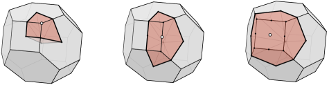
Figure 4. For $p=0$, configurations $\lambda\in\mathcal{X}^{I}/\mathcal{X}=\mathbb{R}^{I}/(1,\dots,1)$ shown in red which respect the composition $G$ shown in white (i.e. $\lambda(i_{1})\vee\!\!\wedge\ \lambda(i_{2})$ for all $(i_{1},i_{2})$ such that $G|_{\{i_{1},i_{2}\}}=(i_{1},i_{2})$), depicted on the tropical toric compactification of the tropical torus $\mathbb{R}^{I}/(1,\dots,1)=(\mathbb{T}^{\times})^{I}/\mathbb{T}^{\times}$ with respect to the braid arrangement fan.

Since $\boldsymbol{\Sigma}$ is the free algebra on $\textbf{E}^{\ast}_{+}$, we have the unique extension to a system of generalized T-products

$$\text{T}:\boldsymbol{\Sigma}\otimes\textbf{E}_{\mathcal{F}_{\text{loc}}[[\hbar]]}\to\textbf{U}_{\mathcal{F}((\hbar))},\qquad\text{T}_{I}(\mathtt{H}_{F}\otimes\emph{{A}}_{I}):=\text{T}_{S_{1}}(\emph{{A}}_{S_{1}})\star_{\text{H}}\dots\star_{\text{H}}\text{T}_{S_{k}}(\emph{{A}}_{S_{k}}).$$

Then:

1. (perturbation) we say that T satisfies perturbation if the singleton components $\text{T}_{i}$ are isomorphic to the inclusion $\mathcal{F}_{\text{loc}}[[\hbar]]\hookrightarrow\mathcal{F}((\hbar))$, that is

   $${\text{T}}_{i}(\emph{{A}})=\,:\!\emph{{A}}\!:$$

2. (causal factorization) we say that T satisfies causal factorization if for all compositions $(S,T)$ of $I$ with two lumps, if $\emph{{A}}_{I}\in\textbf{E}_{\mathcal{F}_{\text{loc}}[[\hbar]]}[I]$ respects $(S,T)$ then

   (48) $$\text{T}_{I}(\mathtt{H}_{(I)}\otimes\emph{{A}}_{I})=\text{T}_{I}(\mathtt{H}_{(S,T)}\otimes\emph{{A}}_{I}).$$

Let a (fully normalized) system of time-ordered products be a system of T-products which satisfies perturbation and causal factorization. The corresponding unique extension of T to $\boldsymbol{\Sigma}$ is called the associated system of generalized time-ordered products. After currying

$$\boldsymbol{\Sigma}\to\mathcal{H}(\textbf{E}_{\mathcal{F}_{\text{loc}}[[\hbar]]},\textbf{U}_{\mathcal{F}((\hbar))}),\qquad\mathtt{H}_{F}\mapsto\text{T}(S_{1})\dots\text{T}(S_{k})$$

the linear maps

$$\text{T}(S_{1})\dots\text{T}(S_{k}):\mathcal{F}_{\text{loc}}[[\hbar]]^{\otimes I}\to\mathcal{F}((\hbar)),\qquad\emph{{A}}_{I}\mapsto\text{T}_{I}(\mathtt{H}_{F}\otimes\emph{{A}}_{I})$$

are called generalized time-ordered products. The linear maps $\text{T}(I)$ are called time-ordered products. After fixing a field polynomial, so that each $\emph{{A}}_{i_{j}}$ of $\emph{{A}}_{I}$ is determined by a bump function $b_{i_{j}}$, they are usually presented in generalized function notation as follows,

$$\text{T}_{I}(\emph{{A}}_{i_{1}}\otimes\cdots\otimes\emph{{A}}_{i_{n}})=\int_{\mathcal{X}^{I}}\text{T}(x_{i_{1}},\dots,x_{i_{n}})b_{i_{1}}(x_{i_{1}})\dots b_{i_{n}}(x_{i_{1}})dx_{i_{1}}\dots dx_{i_{n}}$$

where $(x_{i_{1}},\dots,x_{i_{n}})\mapsto\text{T}(x_{i_{1}},\dots,x_{i_{n}})$ is an “operator-valued” (Wick algebra-valued) generalized function. See e.g. [EG73, Section 1.2]. In the following, recall the Tits product ‘$\,\triangleright$’ from Section 7.7.

Proposition 13.1.

Let

$$\text{T}:\textbf{E}^{\ast}_{+}\otimes\textbf{E}_{\mathcal{F}_{\text{loc}}[[\hbar]]}\to\textbf{U}_{\mathcal{F}((\hbar))}$$

be a system of T-products which satisfies causal factorization. Given a composition $G=(U_{1},\dots,U_{k})$ of $I$, and $\emph{{A}}_{I}\in\textbf{E}_{\mathcal{F}_{\text{loc}}[[\hbar]]}[I]$ which respects $G$, then

$$\text{T}_{I}(\mathtt{a}\otimes\emph{{A}}_{I})=\text{T}_{I}(\mathtt{a}\triangleright\mathtt{H}_{G}\otimes\emph{{A}}_{I})\qquad\text{for all}\quad\mathtt{a}\in\boldsymbol{\Sigma}[I].$$

Proof.

We have

$$\text{T}_{I}(\mathtt{H}_{G}\otimes\emph{{A}}_{I})=\underbrace{\text{T}_{U_{1}}(\emph{{A}}_{U_{1}})\star_{\text{H}}\dots\star_{\text{H}}\text{T}_{U_{k}}(\emph{{A}}_{U_{k}})=\text{T}_{I}(\emph{{A}}_{I})}_{\text{by repeated applications of causal factorization}}.$$

Observe that the action $\mathtt{H}_{F}\mapsto\mathtt{H}_{F}\triangleright\mathtt{H}_{G}$, for $F\in\Sigma[I]$, replaces the lumps of $F$ with their intersections with $G$. But we just saw that $\text{T}_{I}(\emph{{A}}_{I})=\text{T}_{I}(\mathtt{H}_{G}\otimes\emph{{A}}_{I})$, and so it follows that

$$\text{T}_{I}(\mathtt{H}_{F}\otimes\emph{{A}}_{I})=\text{T}_{I}(\mathtt{H}_{F}\triangleright\mathtt{H}_{G}\otimes\emph{{A}}_{I}).$$

Since the claim is true for the $\mathtt{H}$-basis, it is true for all $\mathtt{a}\in\boldsymbol{\Sigma}[I]$. ∎

Corollary 13.1.1.

If $\mathtt{a}\triangleright\mathtt{H}_{G}=0$, then

$$\text{T}_{I}(\mathtt{a}\otimes\emph{{A}}_{I})=0$$

for all $\emph{{A}}_{I}\in\textbf{E}_{\mathcal{F}_{\text{loc}}[[\hbar]]}[I]$ which respect $G$.

The restriction of T to the primitive part Lie algebra is called the associated system of generalized retarded products,

$$\text{R}:\textbf{Zie}\otimes\textbf{E}_{\mathcal{F}_{\text{loc}}[[\hbar]]}\to\mathcal{F}((\hbar)).$$

The image of the Dynkin elements $\mathtt{D}_{\mathcal{S}}$ under the currying of R are the generalized retarded products $\text{R}_{\mathcal{S}}$, see e.g. [EG73, Equation 79]. Combining this with 7.4 and 13.1.1, we see that the generalized retarded products have certain interesting support properties.

Given a system of generalized time-ordered products

$$\text{T}:\boldsymbol{\Sigma}\otimes\textbf{E}_{\mathcal{F}_{\text{loc}}[[\hbar]]}\to\textbf{U}_{\mathcal{F}((\hbar))}$$

the T-exponential $\mathcal{S}=\mathcal{S}_{\mathtt{G}(1/\text{i}\hbar)}$ (defined in (45)) for the group-like series

$$\mathtt{G}(1/\text{i}\hbar):\textbf{E}\to\boldsymbol{\Sigma},\qquad\mathtt{H}_{I}\mapsto\dfrac{1}{\text{i}\hbar}\mathtt{H}_{(I)}$$

is called the associated perturbative S-matrix scheme. Thus, $\mathcal{S}$ is the function

$$\mathcal{S}:\mathcal{F}_{\text{loc}}[[\hbar]]\to\mathcal{F}((\hbar))[[\emph{{j}}\,]],\qquad\emph{{A}}\mapsto\mathcal{S}(\emph{{j}}\,\!\emph{{A}})=\sum^{\infty}_{n=0}\bigg{(}\dfrac{1}{\text{i}\hbar}\bigg{)}^{\!n}\dfrac{\emph{{j}}\,^{n}}{n!}\text{T}_{n}(\emph{{A}}^{n}).$$

Given a choice of vector $\emph{{S}}_{\text{int}}\in\mathcal{F}_{\text{loc}}[[\hbar]]$, now called the adiabatically switched interaction, recall from Section 10.1 that we also have the T-exponential perturbed by the up coderivation of $\textbf{E}^{\ast}$,

$$\mathcal{S}_{\emph{{g}}\emph{{S}}_{\text{int}}}:\mathcal{F}_{\text{loc}}[[\hbar]]\to\mathcal{F}((\hbar))[[\emph{{g}},\!\emph{{j}}\,]],\qquad\emph{{A}}\mapsto\mathcal{S}_{\emph{{g}}\emph{{S}}_{\text{int}}}(\emph{{j}}\,\!\emph{{A}})=\mathcal{S}(\emph{{g}}\emph{{S}}_{\text{int}}+\emph{{j}}\,\!\emph{{A}}).$$

As in [Sch20, Section 15], we may extend $\mathbb{C}[[\hbar,\emph{{g}},\!\emph{{j}}\,]]$-linearly to obtain a map

$$\mathcal{F}_{\text{loc}}[[\hbar,\emph{{g}},\!\emph{{j}}\,]]\langle\emph{{g}},\!\emph{{j}}\,\rangle\to\mathcal{F}((\hbar))[[\emph{{g}},\!\emph{{j}}\,]]$$

where $\mathcal{F}_{\text{loc}}[[\hbar,\emph{{g}},\!\emph{{j}}\,]]\langle\emph{{g}},\!\emph{{j}}\,\rangle$ denotes formal power series which are at least linear in g or j .

14. Interactions

Given a choice of interaction $\emph{{S}}_{\text{int}}\in\mathcal{F}_{\text{loc}}[[\hbar]]$, and a system of fully normalized generalized time-ordered products

$$\text{T}:\boldsymbol{\Sigma}\otimes\textbf{E}_{\mathcal{F}_{\text{loc}}[[\hbar]]}\to\textbf{U}_{\mathcal{F}((\hbar))},$$

we have the new system of interacting generalized time-ordered products which is obtained by applying the construction of Section 6.4 to the retarded Steinmann arrow biderivation $\downarrow(-)$ for $\boldsymbol{\Sigma}$, as considered in Section 10.2,

$$\widetilde{\text{T}}:\boldsymbol{\Sigma}\otimes\textbf{E}_{\mathcal{F}_{\text{loc}}[[\hbar]]}\to\textbf{U}_{\mathcal{F}((\hbar))[[\emph{{g}}]]},\qquad\widetilde{\text{T}}:=\text{T}^{\textbf{E}}\circ\check{\rho}_{\downarrow,\emph{{S}}_{\text{int}}}.$$

The associated generating function scheme $\mathcal{Z}_{\emph{{g}}\emph{{S}}_{\text{int}}}$ for interacting field observables (more generally for time-ordered products of interacting field observables) is the new T-exponential for the group-like series $\mathtt{G}(1/\text{i}\hbar)$, denoted $\mathcal{V}_{\emph{{g}}\emph{{S}}_{\text{int}}}$ in Section 10.2. Thus, $\mathcal{Z}_{\emph{{g}}\emph{{S}}_{\text{int}}}$ is the function

$$\mathcal{Z}_{\emph{{g}}\emph{{S}}_{\text{int}}}:\mathcal{F}_{\text{loc}}[[\hbar]]\to\mathcal{F}((\hbar))[[\emph{{g}},\!\emph{{j}}\,]],\qquad\emph{{A}}\mapsto\mathcal{Z}_{\emph{{g}}\emph{{S}}_{\text{int}}}(\emph{{j}}\,\!\emph{{A}})$$

where

$$\mathcal{Z}_{\emph{{g}}\emph{{S}}_{\text{int}}}(\emph{{j}}\,\!\emph{{A}})\!:=\!\sum_{n=0}^{\infty}\!\bigg{(}\dfrac{1}{\text{i}\hbar}\bigg{)}^{\!\!n}\!\dfrac{\emph{{j}}\,^{n}}{n!}\widetilde{\text{T}}_{n}(\emph{{A}}_{n})=\!\sum_{n=0}^{\infty}\sum_{r=0}^{\infty}\!\bigg{(}\dfrac{1}{\text{i}\hbar}\bigg{)}^{\!\!r+n}\!\dfrac{\emph{{g}}^{r}\emph{{j}}\,^{n}}{r!\,n!}\,\!\text{R}_{r;n}(\emph{{S}}_{\text{int}}^{\,r};\emph{{A}}^{n})=\mathcal{S}^{-1}(\emph{{g}}\emph{{S}}_{\text{int}})\star_{\text{H}}\mathcal{S}(\emph{{g}}\emph{{S}}_{\text{int}}+\emph{{j}}\,\!\emph{{A}}).$$

Then

$$\emph{{A}}_{\text{int}}:=\widetilde{\text{T}}_{i}(\emph{{A}})=\sum_{r=0}^{\infty}\bigg{(}\dfrac{1}{\text{i}\hbar}\bigg{)}^{\!r}\dfrac{\emph{{g}}^{r}}{r!}\text{R}^{r}_{1}(\emph{{S}}^{\,r}_{\text{int}};\emph{{A}})\in\mathcal{F}((\hbar))[[\emph{{g}}]]$$

is the local interacting field observable of A. Bogoliubov’s formula (47) now reads

$$\emph{{A}}_{\text{int}}=\text{i}\hbar\,\dfrac{d}{d\emph{{j}}\,}\Bigr{|}_{\emph{{j}}\,=0}\mathcal{Z}_{\emph{{g}}\emph{{S}}_{\text{int}}}(\emph{{j}}\,\!\emph{{A}}).$$

One views $\emph{{A}}_{\text{int}}$ as the deformation of the local observable A due to the interaction $\emph{{S}}_{\text{int}}$ being turned on. One can show that $\widetilde{\text{T}}$ does indeed land in $\textbf{U}_{\mathcal{F}[[\hbar,\emph{{g}}]]}$ [DF01, Proposition 2 (ii)]. The perturbative interacting quantum field theory then has a classical limit [Col16], [HR20].

15. Scattering Amplitudes

We finish with a translation of a standard result in pAQFT (see [Sch20, Example 15.12]) into our notation, which relates S-matrix schemes as presented in Section 13 to S-matrices used to compute scattering amplitudes, which are predictions of pAQFT that are tested with scattering experiments at particle accelerators.

Following [Düt19, Definition 2.5.2], the Hadamard vacuum state $\langle-\rangle_{0}$ is the linear map given by

$$\langle-\rangle_{0}:\mathcal{F}[[\hbar,\emph{{g}}]]\to\mathbb{C}[[\hbar,\emph{{g}}]],\qquad\emph{{O}}\mapsto\langle\emph{{O}}\,\rangle_{0}:=\emph{{O}}\,(\Phi=0).$$

Let $\emph{{S}}_{\text{int}}\in\mathcal{F}_{\text{loc}}[[\hbar]]$. We say that the Hadamard vacuum state $\langle-\rangle_{0}$ is stable with respect to the interaction $\emph{{S}}_{\text{int}}$ if for all $\emph{{O}}\in\mathcal{F}[[\hbar,\emph{{g}}]]$, we have

(49) $$\big{\langle}\emph{{O}}\star_{\text{H}}\mathcal{S}(\emph{{g}}\emph{{S}}_{\text{int}})\big{\rangle}_{0}=\big{\langle}\emph{{O}}\,\big{\rangle}_{0}\big{\langle}\mathcal{S}(\emph{{g}}\emph{{S}}_{\text{int}})\big{\rangle}_{0}\qquad\text{and}\qquad\big{\langle}\mathcal{S}^{-1}(\emph{{g}}\emph{{S}}_{\text{int}})\star_{\text{H}}\emph{{O}}\,\big{\rangle}_{0}=\dfrac{1}{\big{\langle}\mathcal{S}(\emph{{g}}\emph{{S}}_{\text{int}})\big{\rangle}_{0}}\big{\langle}\emph{{O}}\,\big{\rangle}_{0}.$$

In situations where

$$\emph{{S}}_{\text{int}}\otimes\emph{{A}}_{I}\in\textbf{E}^{\prime}_{\mathcal{F}_{\text{loc}}[[\hbar]]}[I]\qquad\text{respects}\qquad(S,\ast,T)$$

we can interpret free particles/wave packets labeled by $T$ coming in from the far past, interacting in a compact region according to the adiabatically switched interaction $\emph{{S}}_{\text{int}}$, and then emerging into the far future, labeled by $S$. For $\emph{{A}}_{I}\in\textbf{E}_{\mathcal{F}_{\text{loc}}[[\hbar]]}[I]$, let

$$\text{G}_{I}(\emph{{A}}_{I}):=\big{\langle}\widetilde{\text{T}}(\emph{{A}}_{I})\big{\rangle}_{0}.$$

If we fix the field polynomial of local observables to be $\text{P}(\Phi)=\Phi$, then $\emph{{A}}_{I}\mapsto\text{G}_{I}(\emph{{A}}_{I})$ is the time-ordered $n$-point correlation function, or Green’s function. They are usually presented in generalized function notation as follows,

$$\text{G}_{I}(b_{i_{1}}\otimes\cdots\otimes b_{i_{n}})=\int_{\mathcal{X}^{I}}\Big{\langle}\text{T}\big{(}\boldsymbol{\Phi}(x_{i_{1}})\dots\boldsymbol{\Phi}(x_{i_{n}})\big{)}\Big{\rangle}_{0}b_{i_{1}}(x_{i_{1}})\dots b_{i_{n}}(x_{i_{n}})dx_{i_{1}}\dots dx_{i_{n}}.$$

Note that to obtain the true Green’s functions, we still have to take the adiabatic limit.

Proposition 15.1.

If the Hadamard vacuum state $\langle-\rangle_{0}$ is stable with respect to $\emph{{S}}_{\text{int}}\in\mathcal{F}_{\text{loc}}[[\hbar]]$, and if $\emph{{S}}_{\text{int}}\otimes\emph{{A}}_{I}\in\textbf{E}^{\prime}_{\mathcal{F}_{\text{loc}[[\hbar]]}}[I]$ respects the composition $(S,\ast,T)$, then

$$\text{G}_{I}(\emph{{A}}_{I})=\dfrac{1}{\Big{\langle}\mathcal{S}(\emph{{g}}\emph{{S}}_{\text{int}})\Big{\rangle}_{0}}\Big{\langle}\text{T}_{S}(\emph{{A}}_{S})\star_{\text{H}}\mathcal{S}(\emph{{g}}\emph{{S}}_{\text{int}})\star_{\text{H}}\text{T}_{T}(\emph{{A}}_{T})\Big{\rangle}_{0}.$$

Proof.

We have

$$\text{G}_{I}(\emph{{A}}_{I}) =\big{\langle}\widetilde{\text{T}}(\emph{{A}}_{I})\big{\rangle}_{0}$$

$$=\bigg{\langle}\sum_{r=0}^{\infty}\dfrac{\emph{{g}}^{r}}{r!}\text{R}_{r;I}(\emph{{S}}^{\,r}_{\text{int}};\emph{{A}}_{I})\bigg{\rangle}_{0}$$

$$=\bigg{\langle}\sum_{r=0}^{\infty}\sum_{r_{1}+r_{2}=r}\dfrac{\emph{{g}}^{r}}{r_{1}!\,r_{2}!}\overline{\text{T}}^{r_{1}}_{\emptyset}(\emph{{S}}^{\,r_{1}}_{\text{int}})\star_{\text{H}}\text{T}^{r_{2}}_{I}(\emph{{S}}^{\,r_{2}}_{\text{int}}\emph{{A}}_{I})\bigg{\rangle}_{0}.$$

To obtain the final line, we expanded the retarded products according to (46). Then, by causal factorization (48), we have

$$\text{T}^{r_{2}}_{I}(\emph{{S}}^{\,r_{2}}_{\text{int}}\emph{{A}}_{I})=\text{T}_{S}(\emph{{A}}_{S})\star_{\text{H}}\text{T}^{r_{2}}_{\emptyset}(\emph{{S}}^{\,r_{2}}_{\text{int}})\star_{\text{H}}\text{T}_{T}(\emph{{A}}_{T}).$$

Therefore

$$\text{G}_{I}(\emph{{A}}_{I}) =\bigg{\langle}\sum_{r=0}^{\infty}\sum_{r_{1}+r_{2}=r}\dfrac{\emph{{g}}^{r}}{r_{1}!\,r_{2}!}\overline{\text{T}}^{r_{1}}_{\emptyset}(\emph{{S}}^{\,r_{1}}_{\text{int}})\star_{\text{H}}\text{T}_{S}(\emph{{A}}_{S})\star_{\text{H}}\text{T}^{r_{2}}_{\emptyset}(\emph{{S}}^{\,r_{2}}_{\text{int}})\star_{\text{H}}\text{T}_{T}(\emph{{A}}_{T})\bigg{\rangle}_{0}.$$

$$=\bigg{\langle}\sum_{r=0}^{\infty}\dfrac{\emph{{g}}^{r}}{r!}\overline{\text{T}}^{r}_{\emptyset}(\emph{{S}}^{\,r}_{\text{int}})\star_{\text{H}}\text{T}_{S}(\emph{{A}}_{S})\star_{\text{H}}\sum_{r=0}^{\infty}\dfrac{\emph{{g}}^{r}}{r!}\text{T}^{r}_{\emptyset}(\emph{{S}}^{\,r}_{\text{int}})\star_{\text{H}}\text{T}_{T}(\emph{{A}}_{T})\bigg{\rangle}_{0}.$$

$$=\Big{\langle}\mathcal{S}^{-1}(\emph{{g}}\emph{{S}}_{\text{int}})\star_{\text{H}}\text{T}_{S}(\emph{{A}}_{S})\star_{\text{H}}\mathcal{S}(\emph{{g}}\emph{{S}}_{\text{int}})\star_{\text{H}}\text{T}_{T}(\emph{{A}}_{T})\Big{\rangle}_{0}$$

$$=\dfrac{1}{\Big{\langle}\mathcal{S}(\emph{{g}}\emph{{S}}_{\text{int}})\Big{\rangle}_{0}}\Big{\langle}\text{T}_{S}(\emph{{A}}_{S})\star_{\text{H}}\mathcal{S}(\emph{{g}}\emph{{S}}_{\text{int}})\star_{\text{H}}\text{T}_{T}(\emph{{A}}_{T})\Big{\rangle}_{0}.$$

For the final step, we used vacuum stability (49). ∎

References

• [AB08] Peter Abramenko and Kenneth S. Brown. Buildings, volume 248 of Graduate Texts in Mathematics. Springer, New York, 2008. Theory and applications.
• [Abd04] Abdelmalek Abdesselam. Feynman diagrams in algebraic combinatorics. Sém. Lothar. Combin., 49:Art. B49c, 45, 2002/04.
• [AM10] Marcelo Aguiar and Swapneel Mahajan. Monoidal functors, species and Hopf algebras, volume 29 of CRM Monograph Series. American Mathematical Society, Providence, RI, 2010. With forewords by Kenneth Brown, Stephen Chase and André Joyal.
• [AM13] Marcelo Aguiar and Swapneel Mahajan. Hopf monoids in the category of species. In Hopf algebras and tensor categories, volume 585 of Contemp. Math., pages 17–124. Amer. Math. Soc., Providence, RI, 2013.
• [AM17] Marcelo Aguiar and Swapneel Mahajan. Topics in hyperplane arrangements, volume 226 of Mathematical Surveys and Monographs. American Mathematical Society, Providence, RI, 2017.
• [AM20] Marcelo Aguiar and Swapneel Mahajan. Bimonoids for Hyperplane Arrangements, volume 173. Cambridge University Press, 2020.
• [Ara61] Huzihiro Araki. Generalized retarded functions and analytic function in momentum space in quantum field theory. Journal of Mathematical Physics, 2(2):163–177, 1961.
• [Bar78] M. G. Barratt. Twisted Lie algebras. In Geometric applications of homotopy theory (Proc. Conf., Evanston, Ill., 1977), II, volume 658 of Lecture Notes in Math., pages 9–15. Springer, Berlin, 1978.
• [Bär15] Christian Bär. Green-hyperbolic operators on globally hyperbolic spacetimes. Comm. Math. Phys., 333(3):1585–1615, 2015.
• [BC19] Francisco Borges and Freddy Cachazo. Generalized planar Feynman diagrams: collections. arXiv preprint arXiv:1910.10674, 2019.
• [BDF09] R. Brunetti, M. Dütsch, and K. Fredenhagen. Perturbative algebraic quantum field theory and the renormalization groups. Adv. Theor. Math. Phys., 13(5):1541–1599, 2009.
• [BF00] Romeo Brunetti and Klaus Fredenhagen. Microlocal analysis and interacting quantum field theories: renormalization on physical backgrounds. Comm. Math. Phys., 208(3):623–661, 2000.
• [Bjo15] Anders Bjorner. Positive sum systems. In Combinatorial methods in topology and algebra, volume 12 of Springer INdAM Ser., pages 157–171. Springer, Cham, 2015.
• [BK05] Christoph Bergbauer and Dirk Kreimer. The Hopf algebra of rooted trees in Epstein-Glaser renormalization. Ann. Henri Poincaré, 6(2):343–367, 2005.
• [BL75] J. Bros and M. Lassalle. Analyticity properties and many-particle structure in general quantum field theory. II. One-particle irreducible $n$-point functions. Comm. Math. Phys., 43(3):279–309, 1975.
• [BLL98] F. Bergeron, G. Labelle, and P. Leroux. Combinatorial species and tree-like structures, volume 67 of Encyclopedia of Mathematics and its Applications. Cambridge University Press, Cambridge, 1998. Translated from the 1994 French original by Margaret Readdy, with a foreword by Gian-Carlo Rota.
• [BMM+12] L.J. Billera, J. Tatch Moore, C. Dufort Moraites, Y. Wang, and K. Williams. Maximal unbalanced families. arXiv preprint arXiv:1209.2309, 2012.
• [Bor11] Richard E. Borcherds. Renormalization and quantum field theory. Algebra Number Theory, 5(5):627–658, 2011.
• [BP99] Alexander Barvinok and James E. Pommersheim. An algorithmic theory of lattice points in polyhedra. In New perspectives in algebraic combinatorics (Berkeley, CA, 1996–97), volume 38 of Math. Sci. Res. Inst. Publ., pages 91–147. Cambridge Univ. Press, Cambridge, 1999.
• [Bro09] Christian Brouder. Quantum field theory meets Hopf algebra. Math. Nachr., 282(12):1664–1690, 2009.
• [Bro17] Francis Brown. Feynman amplitudes, coaction principle, and cosmic Galois group. Commun. Number Theory Phys., 11(3):453–556, 2017.
• [BS59] N. N. Bogoliubov and D. V. Shirkov. Introduction to the theory of quantized fields. Authorized English edition. Revised and enlarged by the authors. Translated from the Russian by G. M. Volkoff. Interscience Monographs in Physics and Astronomy, Vol. III. Interscience Publishers, Inc., New York; Interscience Publishers Ltd., London, 1959.
• [CGUZ19] Freddy Cachazo, Alfredo Guevara, Bruno Umbert, and Yong Zhang. Planar matrices and arrays of Feynman diagrams. arXiv preprint arXiv:1912.09422, 2019.
• [CHDD+19] Simon Caron-Huot, Lance J Dixon, Falko Dulat, Matt Von Hippel, Andrew J McLeod, and Georgios Papathanasiou. The cosmic Galois group and extended Steinmann relations for planar N=4 SYM amplitudes. Journal of High Energy Physics, 2019(9):61, 2019.
• [CHDD+20] Simon Caron-Huot, Lance J. Dixon, James M. Drummond, Falko Dulat, Jack Foster, Ömer Gürdoğan, Matt von Hippel, Andrew J. McLeod, and Georgios Papathanasiou. The Steinmann Cluster Bootstrap for $N=4$ Super Yang-Mills Amplitudes. PoS, CORFU2019:003, 2020.
• [CJ70] John T. Cannon and Arthur M. Jaffe. Lorentz covariance of the $\lambda(\varphi^{4})_{2}$ quantum field theory. Comm. Math. Phys., 17:261–321, 1970.
• [Col16] Giovanni Collini. Fedosov quantization and perturbative quantum field theory. arXiv preprint arXiv:1603.09626, 2016.
• [DF01] M. Dütsch and K. Fredenhagen. Algebraic quantum field theory, perturbation theory, and the loop expansion. Comm. Math. Phys., 219(1):5–30, 2001.
• [DF04] Michael Dütsch and Klaus Fredenhagen. Causal perturbation theory in terms of retarded products, and a proof of the action Ward identity. Rev. Math. Phys., 16(10):1291–1348, 2004.
• [DFG18] James Drummond, Jack Foster, and Ömer Gürdoğan. Cluster adjacency properties of scattering amplitudes in N=4 supersymmetric Yang-Mills theory. Physical review letters, 120(16):161601, 2018.
• [DFKR14] Michael Dütsch, Klaus Fredenhagen, Kai Johannes Keller, and Katarzyna Rejzner. Dimensional regularization in position space and a forest formula for Epstein-Glaser renormalization. J. Math. Phys., 55(12):122303, 37, 2014.
• [Düt12] Michael Dütsch. Connection between the renormalization groups of Stückelberg-Petermann and Wilson. Confluentes Math., 4(1):1240001, 16, 2012.
• [Düt19] Michael Dütsch. From classical field theory to perturbative quantum field theory, volume 74 of Progress in Mathematical Physics. Birkhäuser/Springer, Cham, 2019. With a foreword by Klaus Fredenhagen.
• [Dys52] F. J. Dyson. Divergence of perturbation theory in quantum electrodynamics. Phys. Rev. (2), 85:631–632, 1952.
• [Ear19] Nick Early. Planar kinematic invariants, matroid subdivisions and generalized Feynman diagrams. arXiv preprint arXiv:1912.13513, 2019.
• [EG73] H. Epstein and V. Glaser. The role of locality in perturbation theory. Ann. Inst. H. Poincaré Sect. A (N.S.), 19:211–295 (1974), 1973.
• [EGS75] H. Epstein, V. Glaser, and R. Stora. General properties of the n-point functions in local quantum field theory. In Institute on Structural Analysis of Multiparticle Collision Amplitudes in Relativistic Quantum Theory Les Houches, France, June 3-28, 1975, pages 5–93, 1975.
• [Eps16] Henri Epstein. Trees. Nuclear Phys. B, 912:151–171, 2016.
• [Far11] William G. Faris. Combinatorial species and Feynman diagrams. Sém. Lothar. Combin., 61A:Art. B61An, 37, 2009/11.
• [Fau01] Bertfried Fauser. On the Hopf algebraic origin of Wick normal ordering. J. Phys. A, 34(1):105–115, 2001.
• [GBL00] Jose M Gracia-Bondia and Serge Lazzarini. Connes-Kreimer-Epstein-Glaser renormalization. arXiv preprint hep-th/0006106v2, 2000.
• [GJ68] James Glimm and Arthur Jaffe. A $\lambda\phi^{4}$ quantum field without cutoffs. I. Phys. Rev. (2), 176:1945–1951, 1968.
• [GJS74] James Glimm, Arthur Jaffe, and Thomas Spencer. The Wightman axioms and particle structure in the ${\mathscr{P}}(\phi)_{2}$ quantum field model. Ann. of Math. (2), 100:585–632, 1974.
• [GK18] John Gough and Joachim Kupsch. Quantum fields and processes, volume 171 of Cambridge Studies in Advanced Mathematics. Cambridge University Press, Cambridge, 2018. A combinatorial approach.
• [GLZ57] V. Glaser, H. Lehmann, and W. Zimmermann. Field operators and retarded functions. Nuovo Cimento (10), 6:1122–1128, 1957.
• [HK64] Rudolf Haag and Daniel Kastler. An algebraic approach to quantum field theory. J. Mathematical Phys., 5:848–861, 1964.
• [Hol08] Stefan Hollands. Renormalized quantum Yang-Mills fields in curved spacetime. Rev. Math. Phys., 20(9):1033–1172, 2008.
• [HR20] Eli Hawkins and Kasia Rejzner. The star product in interacting quantum field theory. Lett. Math. Phys., 110(6):1257–1313, 2020.
• [IS78] V. A. Ilyin and D. A. Slavnov. Algebras of observables in the $S$-matrix approach. Teoret. Mat. Fiz., 36(1):32–41, 1978.
• [Joy81] André Joyal. Une théorie combinatoire des séries formelles. Adv. in Math., 42(1):1–82, 1981.
• [Joy86] André Joyal. Foncteurs analytiques et espèces de structures. In Combinatoire énumérative (Montreal, Que., 1985/Quebec, Que., 1985), volume 1234 of Lecture Notes in Math., pages 126–159. Springer, Berlin, 1986.
• [LM00] A. Losev and Y. Manin. New moduli spaces of pointed curves and pencils of flat connections. volume 48, pages 443–472. 2000. Dedicated to William Fulton on the occasion of his 60th birthday.
• [LNO19] Zhengwei Liu, William Norledge, and Adrian Ocneanu. The adjoint braid arrangement as a combinatorial Lie algebra via the Steinmann relations. arXiv preprint arXiv:1901.03243, 2019.
• [NO19] William Norledge and Adrian Ocneanu. Hopf monoids, permutohedral cones, and generalized retarded functions. to appear in Annals IHP D - Comb., Phys. and their Interactions, 2019.
• [Ocn18] Adrian Ocneanu. Higher Representation Theory. Physics 267, Fall 2017 Harvard Course, and supplementary materials and presentations, 2017-2018. The course is available on YouTube, and supplementary materials are in preparation for publication.
• [Pin00] G. Pinter. The Hopf algebra structure of Connes and Kreimer in Epstein-Glaser renormalization. Lett. Math. Phys., 54(3):227–233, 2000.
• [Pol58] J. C. Polkinghorne. Generalized retarded products. Proc. Roy. Soc. London Ser. A, 247:557–561, 1958.
• [PS16] G. Popineau and R. Stora. A pedagogical remark on the main theorem of perturbative renormalization theory. Nuclear Phys. B, 912:70–78, 2016.
• [Rej16] Kasia Rejzner. Perturbative algebraic quantum field theory. Mathematical Physics Studies. Springer, Cham, 2016. An introduction for mathematicians.
• [Rue61] D. Ruelle. Connection between Wightman functions and Green functions in $p$-space. Nuovo Cimento (10), 19:356–376, 1961.
• [Sch93] William R. Schmitt. Hopf algebras of combinatorial structures. Canad. J. Math., 45(2):412–428, 1993.
• [Sch95] G. Scharf. Finite quantum electrodynamics. Texts and Monographs in Physics. Springer-Verlag, Berlin, second edition, 1995. The causal approach.
• [Sch18] Konrad Schultka. Toric geometry and regularization of Feynman integrals. arXiv preprint arXiv:1806.01086, 2018.
• [Sch20] Urs Schreiber. Geometry of physics - perturbative quantum field theory. https://ncatlab.org/nlab/show/geometry+of+physics+--+perturbative+quantum+field+theory, September 2020. Revision 197.
• [Ste60a] Othmar Steinmann. Über den Zusammenhang zwischen den Wightmanfunktionen und den retardierten Kommutatoren. Helv. Phys. Acta, 33:257–298, 1960.
• [Ste60b] Othmar Steinmann. Wightman-Funktionen und retardierte Kommutatoren. II. Helv. Phys. Acta, 33:347–362, 1960.
• [Ste71] Othmar Steinmann. Perturbation expansions in axiomatic field theory. Springer-Verlag, Berlin-New York, 1971. Lecture Notes in Physics, Vol. 11.
• [Sto93a] R Stora. Differential algebras in Lagrangean field theory. ETH-Zürich Lectures, 1993.
• [Sto93b] Christopher R. Stover. The equivalence of certain categories of twisted Lie and Hopf algebras over a commutative ring. J. Pure Appl. Algebra, 86(3):289–326, 1993.
• [SZ11] Sergey Shadrin and Dimitri Zvonkine. A group action on Losev-Manin cohomological field theories. In Annales de l’Institut Fourier, volume 61, pages 2719–2743, 2011.
• [Tit74] Jacques Tits. Buildings of spherical type and finite BN-pairs. Lecture Notes in Mathematics, Vol. 386. Springer-Verlag, Berlin-New York, 1974.