Deep learning regression for inverse quantum scattering
Abstract
In this work we study the inverse quantum scattering via deep learning regression, which is implemented via a Multilayer Perceptron. A step-by-step method is provided in order to obtain the potential parameters. A circular boundary-wall potential was chosen to exemplify the method. Detailed discussion about the training is provided. A investigation with noisy data is presented and it is observed that the neural network is useful to predict the potential parameters.
I Introduction
Machine Learning is a collection of powerful tools that predicts parameters or classify features based on experimental or synthetic data. A plethora of applications exist, such as the reconstruction of porous media [1], feature selection by mutual information [2], percolation and fracture propagation in disordered solids [3], the behavior of Ising spin-lattice [4], a model for turbulent fluxes that recovers spontaneous zonal flow [5], classification of complex features in diffraction images [6] and much more [7, 8, 9].
Recently, two-dimensional quantum scattering is receiving attention, E. de Prunelé gave a formulation for non-isotropic interactions localized on a circle [10]. Maioli et al found analytic solutions for the wavefunction scattered by circular and elliptic billiards [11, 12] and presented a scattering with two-potential formalism [13]. They used a boundary-wall potential introduced by M. G. E. da Luz et al [14]. Which is useful to find analytic solutions for the matrix, the eigenstates, and the scattering solutions for billiards[15]. Along these lines, the BWM provides a significant way to study quantum scattering and electromagnetic wave propagation for TE or TM modes due to the analogy of both physical phenomena [16]. On the other hand, inverse scattering problems have a significant role in applied physics, such as the reconstruction of medium properties [17]. In this scenario, G. Ariel and H. Diamant [18] showed a method to infer the entropy from the structure factor (which can be obtained by quantum scattering), and T. Tyni numerically investigated the two-dimensional inverse scattering with the aid of Saito’s uniqueness theorem [19]. G. Fotopoulos and M. Harju [20] study how to retrieve the singularities of an unknown potential using the Born approximation.
The purpose is to provide a simple method that obtains the potential parameters based on the scattering data. This type of inverse problem is extensively frequent in scattering physics. It is designated a regression problem in the machine learning vocabulary. The method consists in choosing a potential that models the physical system, then generating synthetic data to train a neural network. Hence, we select a circular boundary wall potential. This geometry is reasonable because we know the analytic solutions for the eigenstates and the scattered states[11].
It is well-known that implementing a neural network to solve a regression problem is considered exceedingly good, and the results improve as one adds more hidden layers. However, it can be computationally exhaustive and hard to converge the network’s parameters due to the vanishing gradient problem. Therefore we show how to avoid the last difficulty. The trained neural network can predict the correct results even with noisy input data, and the training set is noiseless.
This paper is organized as follows. In Section II we present the method, including how the synthetic data was generated (subsection II.2) and the neural network training (subsection II.4). In section III, it is shown that the trained neural network can predict the correct values for the potential parameters. Finally, we conclude the discussions in section IV.
II The method
The main idea is to provide a fast way to find the potential parameters due to the scattering cross length obtained for the two-dimensional quantum scattering. The scattering cross length is the two-dimensional analog of the scattering cross-section, the usual formulation can be found at [21, 22, 23] and a comparison between 2D and 3D formulas [24]. The method embraces a few simple steps, and some hints follow the example selected throughout this work. The steps are:
-
1.
Choose the potential that suits the desired physical system.
-
2.
Generate synthetic data that will be the input of the neural network. One can use the scattering cross length and other physical information, such as the particle’s mass, Plank’s constant, etc. Therefore, the output is the potential parameters.
-
3.
Build a neural network. The size of the input will be the number of physical quantities necessary to perform the regression.
-
4.
Train the neural network with synthetic data.
II.1 First Step: Boundary wall potential
Here we use a circular boundary-wall potential that is defined as a line integral
| (1) |
where is the strength function, which we set to be constant , is a circle of radius , the is the two-dimensional Dirac delta. Writing the potential as a Riemann integral, we have
| (2) |
one can see that the parameters and uniquely define this type of potential, therefore those are the ones which we need to predict.
II.2 Second step: Synthetic data
In this subsection is presented an expression for the scattering cross length . It will be employed to generate the synthetic data. Therefore, it is obtained through the analytic solution of the Lippmann-Schwinger equation outside the circle () [11],
| (3) |
where and are the Bessel and Hankel functions of the first kind of order , respectively, is the angle between the wave vector of the plane wave and the axis, and
| (4) |
where . For the sake of simplicity, we set , then using the relation and one can rewrite the eq. (3)
| (5) |
where the sum of Bessel functions was identified as the exponential. Along these lines, one can use the asymptotic expansion of the Hankel function
| (6) |
then it is easy to find the scattering amplitude using
| (7) |
therefore
| (8) |
For central potentials, it is useful to apply the partial wave analysis,
| (9) |
where
| (10) |
and is the phase shift. One can find an analytic expression for the phase shift after combining eq. (8), (9) and (10)
| (11) |
and a relation for the scattering cross length
| (12) |
where stands for the Real part of . For a chosen and it is computed for several values of . It begins with and ends at with increments , and it is used natural units . The series of eq. (12) was truncated at
| (13) |
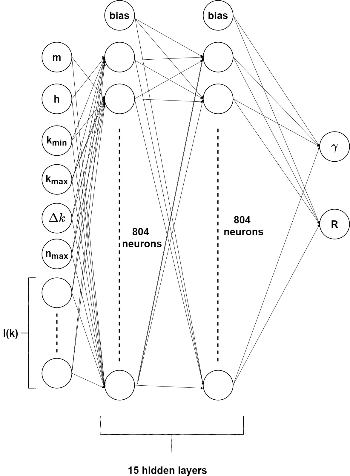
So, one synthetic data is the group of values . Those values are organized as a column vector and are the input of the neural network. Therefore, we generate synthetic data, for different values of and , where spams from to with steps of , and from to with increment .
II.3 Third Step: Build a neural network
Choosing a specific Neural Network to implement a regression problem is decisive due to the antagonism between the computational time to execute the program and the spend personal time desired to obtain the solution. Among several types of Neural Networks (such as Recurrent Neural Networks, Modular Neural Networks, Convolutional Neural Networks, and more), we choose a Multilayer Perceptron because it has a simple setup and provides excellent results. The number of hidden layers in this work () is justified at the subsection II.4. Usually, the more hidden layer in the network better is the results, until it starts to overfit. However, for hidden neurons, one can employ the rules[25]:
-
•
The number of hidden neurons should be between the size of the input layer and the size of the output layer.
-
•
The number of hidden neurons should be 2/3 the size of the input layer, plus the size of the output layer.
-
•
The number of hidden neurons should be less than twice the size of the input layer.
The chosen number in this example was the size of the input plus one-third of it (), and the activation function was the logistic sigmoid.
II.4 Fourth Step: The Training
To train the neural network, the synthetic data were randomly separated among three groups, namely the training set, validation set, and test set. The test set has of the total number of synthetic data. The remaining () was allocated between the training and validation sets. of it for the validation set and to the training set. This separation is important to check the accuracy of the network. The error (loss or cost) function employed is the mean squared difference
| (14) |
where is the network output, is the size of the output and is the desired output, in other words, the and used to produce . The training method is the stochastic gradient descent with a batch size of examples, where is important to apply an adaptive learning rate that is invariant to diagonal rescaling of the gradients [26]. However, one should avoid training the neural network directly, because of the vanishing gradient problem. This leads to a network with high bias.
It is known, that a cascade-correlation learning architecture [27] solves this problem. The procedure consists in training the network several times, first with only one hidden layer. Then, one adds another hidden layer and keeps the weights learned previously. At each training, one must check the convergence of the error over the test set and the validation set. If the error calculated over the validation set increases (over each iteration at one training), then you have overfitting. To solve this problem decrease the number of hidden neurons. Finally, it is imperative to apply the network over the test set at the end of each training, because one can visualize the error decreasing until reaching the desired value. In this work, we stop at hidden layers and obtain an error over the test set of . One can go further (more hidden layers) but this is enough for the purpose of this work.
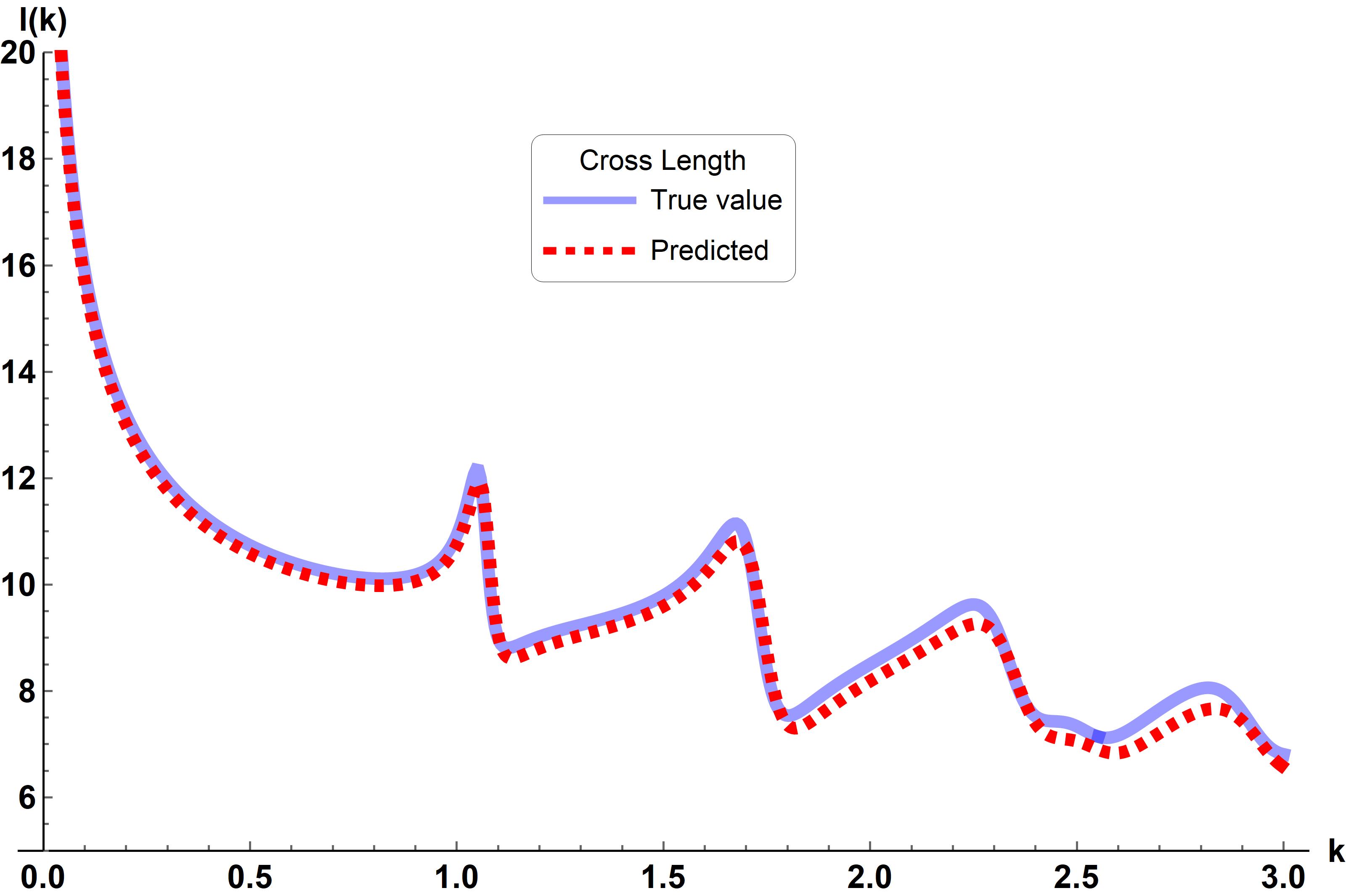
After checking the convergence of the parameters, we repeat the training with all the synthetic data. As an example, in Fig. 2 is plotted the scattering cross length calculated considering and (blue full line). Then, it is provided to the neural network as an input, and it “predicts” the values and . Consequently, is plotted the scattering cross length computed with those values (red dashed line). We calculate the percentage relative difference
| (15) |
where and stands for the “predicted” values obtained by the neural network.
III Prediction with noise
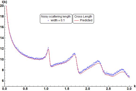
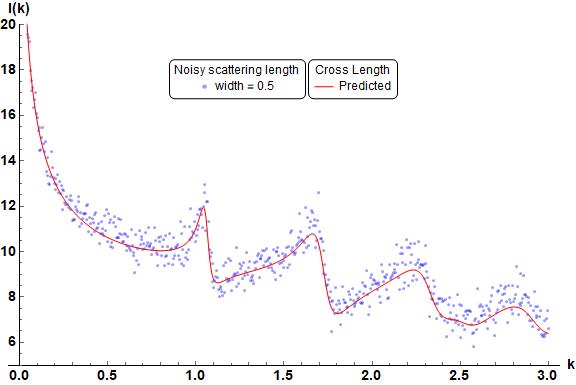
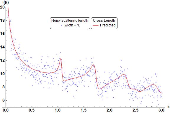
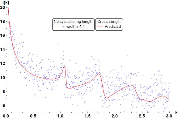
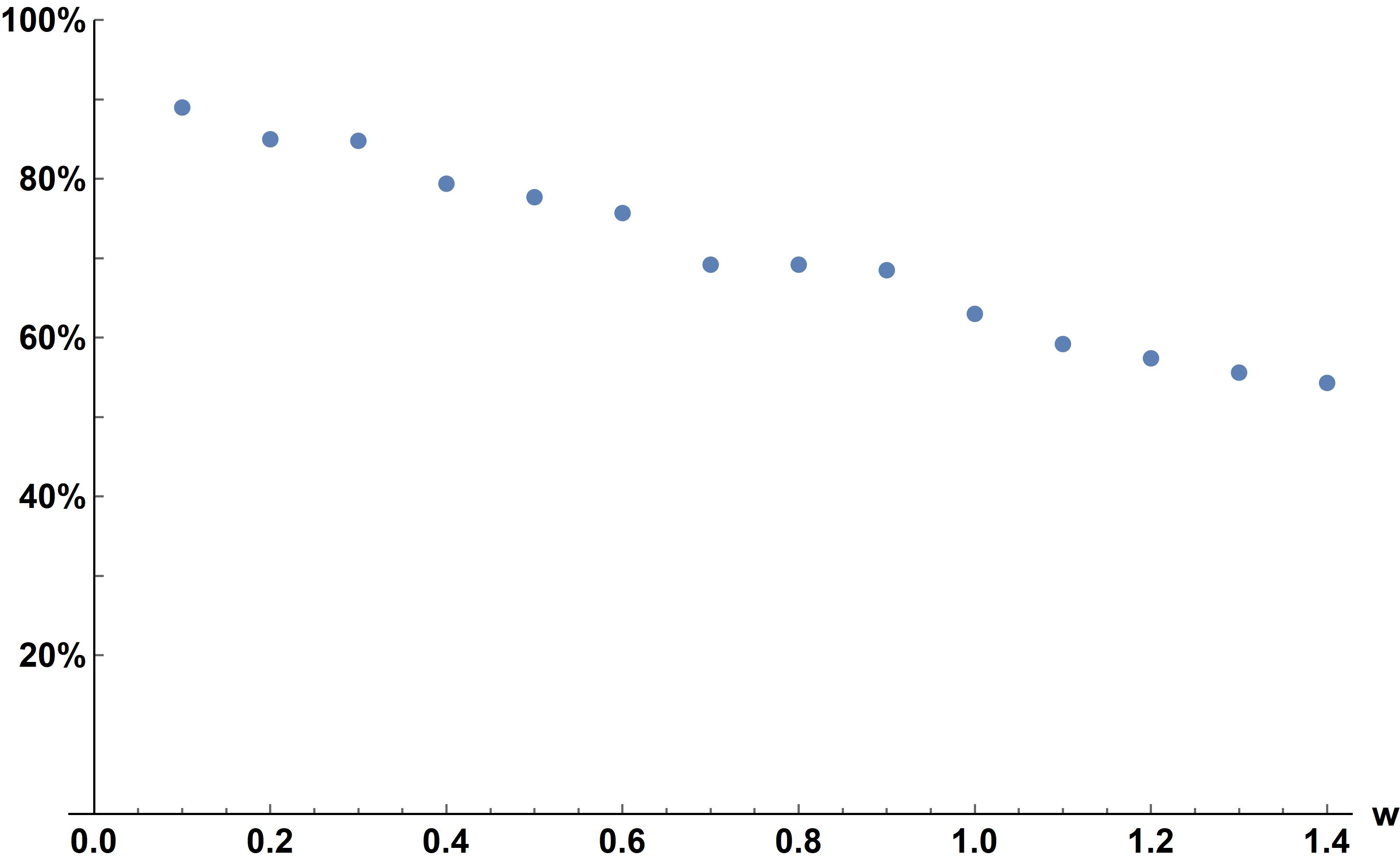
The trained neural network can predict accurate values of parameters when the input data has noise. It generated synthetic data and added Gaussian white noise with different widths. Therefore, it was plotted (Fig. 3) the noisy scattering cross length with its respective prediction to elucidate the procedure. The four plots correspond to the same scattering cross length (same as presented in Fig.2), although their difference is the noise width. Along these lines, each example from Fig. 3 has a correct prediction for the potential parameters. Here we consider a correct prediction as a percentage relative difference less than for all the parameters. Then, it was generated one thousand examples for each width of the noise, where the parameters were randomly selected between the interval and . In Fig. 3 is plotted the percentage of correct predictions for each noise width . It is shown a decrease in accurate predictions as the value of the noise increase.
IV Conclusion
In this work, we have shown how a simple neural network can predict correct values for potential parameters. We choose a circular boundary-wall potential due to the existence of the analytic solution for the wave function and the scattering cross length. However, the vast majority of potential does not have an analytic solution for the wavefunction nor the scattering cross length (or scattering cross section in 3D problems). Consequently one can obtain it via numeric (boundary integral methods) or approximate (Born approximation) methods. The neural network is able to determine the parameters even with noisy input.
References
- Mosser et al. [2017] L. Mosser, O. Dubrule, and M. J. Blunt, Reconstruction of three-dimensional porous media using generative adversarial neural networks, Phys. Rev. E 96, 043309 (2017).
- Kwak and Chong-Ho Choi [2002] N. Kwak and Chong-Ho Choi, Input feature selection by mutual information based on parzen window (2002).
- Kamrava et al. [2020] S. Kamrava, P. Tahmasebi, M. Sahimi, and S. Arbabi, Phase transitions, percolation, fracture of materials, and deep learning, Phys. Rev. E 102, 011001(R) (2020).
- Koch et al. [2020] E. M. Koch, A. M. Koch, N. Kastanos, and L. Cheng, Short-sighted deep learning, Phys. Rev. E 102, 013307 (2020).
- Heinonen and Diamond [2020] R. A. Heinonen and P. H. Diamond, Turbulence model reduction by deep learning, Phys. Rev. E 101, 061201(R) (2020).
- Zimmermann et al. [2019] J. Zimmermann, B. Langbehn, R. Cucini, M. Di Fraia, P. Finetti, A. C. LaForge, T. Nishiyama, Y. Ovcharenko, P. Piseri, O. Plekan, K. C. Prince, F. Stienkemeier, K. Ueda, C. Callegari, T. Möller, and D. Rupp, Deep neural networks for classifying complex features in diffraction images, Phys. Rev. E 99, 063309 (2019).
- Vargas-Hernández et al. [2019] R. A. Vargas-Hernández, Y. Guan, D. H. Zhang, and R. V. Krems, Bayesian optimization for the inverse scattering problem in quantum reaction dynamics, New Journal of Physics 21, 022001 (2019).
- Yao et al. [2019] H. M. Yao, W. E. I. Sha, and L. Jiang, Two-step enhanced deep learning approach for electromagnetic inverse scattering problems, IEEE Antennas and Wireless Propagation Letters 18, 2254 (2019).
- Palffy et al. [2020] A. Palffy, J. Dong, J. F. P. Kooij, and D. M. Gavrila, Cnn based road user detection using the 3d radar cube, IEEE Robotics and Automation Letters 5, 1263 (2020).
- de Prunelé [2018] E. de Prunelé, Two-dimensional quantum scattering by non-isotropic interactions localized on a circle, applications to open billiards, Journal of Mathematical Physics 59, 102102 (2018).
- Maioli and Schmidt [2018] A. C. Maioli and A. G. M. Schmidt, Exact solution to Lippmann-Schwinger equation for a circular billiard, Journal of Mathematical Physics 59, 122102 (2018).
- Maioli and Schmidt [2019a] A. C. Maioli and A. G. Schmidt, Exact solution to the Lippmann-Schwinger equation for an elliptical billiard, Physica E: Low-dimensional Systems and Nanostructures 111, 51 (2019a).
- Maioli and Schmidt [2019b] A. C. Maioli and A. G. M. Schmidt, Two-dimensional scattering by boundary-wall and linear potentials, Physica Scripta 10.1088/1402-4896/ab57e6 (2019b).
- da Luz et al. [1997] M. G. E. da Luz, A. S. Lupu-Sax, and E. J. Heller, Quantum scattering from arbitrary boundaries, Physical Review E 56, 2496 (1997).
- Zanetti et al. [2008] F. M. Zanetti, E. Vicentini, and M. G. da Luz, Eigenstates and scattering solutions for billiard problems: A boundary wall approach, Annals of Physics 323, 1644 (2008).
- Zanetti et al. [2009] F. M. Zanetti, M. L. Lyra, F. a. B. F. de Moura, and M. G. E. da Luz, Resonant scattering states in 2D nanostructured waveguides: a boundary wall approach, Journal of Physics B: Atomic, Molecular and Optical Physics 42, 025402 (2009).
- Rizzuti and Gisolf [2017] G. Rizzuti and A. Gisolf, An iterative method for 2d inverse scattering problems by alternating reconstruction of medium properties and wavefields: theory and application to the inversion of elastic waveforms, Inverse Problems 33, 035003 (2017).
- Ariel and Diamant [2020] G. Ariel and H. Diamant, Inferring entropy from structure, Phys. Rev. E 102, 022110 (2020).
- Tyni [2020] T. Tyni, Numerical results for saito’s uniqueness theorem in inverse scattering theory, Inverse Problems 36, 065002 (2020).
- Fotopoulos and Harju [2017] G. Fotopoulos and M. Harju, Inverse scattering with fixed observation angle data in 2d, Inverse Problems in Science and Engineering 25, 1492 (2017).
- Lapidus [1982] I. R. Lapidus, Quantum‐mechanical scattering in two dimensions, American Journal of Physics 50, 45 (1982).
- Maurone and Lim [1983] P. A. Maurone and T. K. Lim, More on two‐dimensional scattering, American Journal of Physics 51, 856 (1983).
- Adhikari [1986] S. K. Adhikari, Quantum scattering in two dimensions, American Journal of Physics 54, 362 (1986), 1601.02657 .
- De Prunelé [2006] E. De Prunelé, Solvable quantum mechanical model in two-dimensional space, Journal of Physics A: Mathematical and General 39, 12469 (2006).
- Heaton [2015] J. Heaton, Artificial Intelligence for Humans, Volume 3: Deep Learning and Neural Networks, Artificial Intelligence for Humans (Createspace Independent Publishing Platform, 2015).
- Kingma and Ba [2017] D. P. Kingma and J. Ba, Adam: A method for stochastic optimization (2017), arXiv:1412.6980 [cs.LG] .
- Fahlman and Lebiere [1997] S. Fahlman and C. Lebiere, The cascade-correlation learning architecture, Advances in Neural Information Processing Systems 2 (1997).