Cmax++ : Leveraging Experience in Planning and Execution using Inaccurate Models

Abstract

Given access to accurate dynamical models, modern planning approaches are effective in computing feasible and optimal plans for repetitive robotic tasks. However, it is difficult to model the true dynamics of the real world before execution, especially for tasks requiring interactions with objects whose parameters are unknown. A recent planning approach, Cmax, tackles this problem by adapting the planner online during execution to bias the resulting plans away from inaccurately modeled regions. Cmax, while being provably guaranteed to reach the goal, requires strong assumptions on the accuracy of the model used for planning and fails to improve the quality of the solution over repetitions of the same task. In this paper we propose Cmax++, an approach that leverages real-world experience to improve the quality of resulting plans over successive repetitions of a robotic task. Cmax++ achieves this by integrating model-free learning using acquired experience with model-based planning using the potentially inaccurate model. We provide provable guarantees on the completeness and asymptotic convergence of Cmax++ to the optimal path cost as the number of repetitions increases. Cmax++ is also shown to outperform baselines in simulated robotic tasks including 3D mobile robot navigation where the track friction is incorrectly modeled, and a 7D pick-and-place task where the mass of the object is unknown leading to discrepancy between true and modeled dynamics.

1 Introduction

We often require robots to perform tasks that are highly repetitive, such as picking and placing objects in assembly tasks and navigating between locations in a warehouse. For such tasks, robotic planning algorithms have been highly effective in cases where system dynamics is easily specified by an efficient forward model (Berenson, Abbeel, and Goldberg 2012). However, for tasks involving interactions with objects, dynamics are very difficult to model without complete knowledge of the parameters of the objects such as mass and friction (Ji and Xiao 2001). Using inaccurate models for planning can result in plans that are ineffective and fail to complete the task (McConachie et al. 2020). In addition for such repetitive tasks, we expect the robot’s task performance to improve, leading to efficient plans in later repetitions. Thus, we need a planning approach that can use potentially inaccurate models while leveraging experience from past executions to complete the task in each repetition, and improve performance across repetitions.

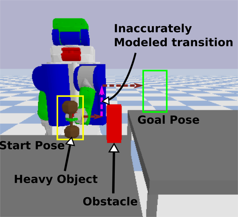
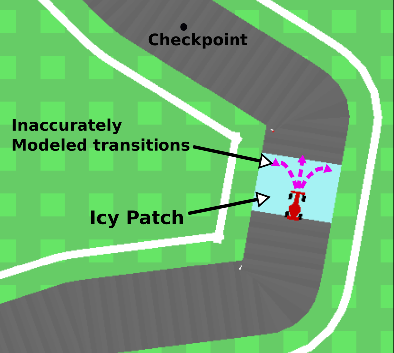
Figure 1: (left) PR2 lifting a heavy dumbbell, that is modeled as light, to a goal location that is higher than the start location resulting in dynamics that are inaccurately modeled (right) Mobile robot navigating around a track with icy patches with unknown friction parameters leading to the robot skidding. In both cases, any path to the goal needs to contain a transition (pink) whose dynamics are not modeled accurately.

A recent planning approach, Cmax, introduced in (Vemula et al. 2020) adapts its planning strategy online to account for any inaccuracies in the forward model without requiring any updates to the dynamics of the model. Cmax achieves this online by inflating the cost of any transition that is found to be incorrectly modeled and replanning, thus biasing the resulting plans away from regions where the model is inaccurate. It does so while maintaining guarantees on completing the task, without any resets, in a finite number of executions. However, Cmax requires that there always exists a path from the current state of the robot to the goal containing only transitions that have not yet been found to be incorrectly modeled. This is a strong assumption on the accuracy of the model and can often be violated, especially in the context of repetitive tasks.

For example, consider the task shown in Figure 1(left) where a robotic arm needs to repeatedly pick a heavy object, that is incorrectly modeled as light, and place it on top of a taller table while avoiding an obstacle. As the object is heavy, transitions that involve lifting the object will have discrepancy between true and modeled dynamics. However, any path from the start pose to the goal pose requires lifting the object and thus, the resulting plan needs to contain a transition that is incorrectly modeled. This violates the aforementioned assumption of Cmax and it ends up inflating the cost of any transition that lifts the object, resulting in plans that avoid lifting the object in future repetitions. Thus, the quality of Cmax solution deteriorates across repetitions and, in some cases, it even fails to complete the task. Figure 1(right) presents another example task where a mobile robot is navigating around a track with icy patches that have unknown friction parameters. Once the robot enters a patch, any action executed results in the robot skidding, thus violating the assumption of Cmax because any path to the goal from current state will have inaccurately modeled transitions. Cmax ends up inflating the cost of all actions executed inside the icy patch, leading to the robot being unable to find a path in future laps and failing to complete the task. Thus, in both examples, we need a planning approach that allows solutions to contain incorrectly modeled transitions while ensuring that the robot reaches the goal.

In this paper we present Cmax++, an approach for interleaving planning and execution that uses inaccurate models and leverages experience from past executions to provably complete the task in each repetition without any resets. Furthermore, it improves the quality of solution across repetitions. In contrast to Cmax, Cmax++ requires weaker conditions to ensure task completeness, and is provably guaranteed to converge to a plan with optimal cost as the number of repetitions increases. The key idea behind Cmax++ is to combine the conservative behavior of Cmax that tries to avoid incorrectly modeled regions with model-free Q-learning that tries to estimate and follow the optimal cost-to-goal value function with no regard for any discrepancies between modeled and true dynamics. This enables Cmax++ to compute plans that utilize inaccurately modeled transitions, unlike Cmax. Based on this idea, we present an algorithm for small state spaces, where we can do exact planning, and a practical algorithm for large state spaces using function approximation techniques. We also propose an adaptive version of Cmax++ that intelligently switches between Cmax and Cmax++ to combine the advantages of both approaches, and exhibits goal-driven behavior in earlier repetitions and optimality in later repetitions. The proposed algorithms are tested on simulated robotic tasks: 3D mobile robot navigation where the track friction is incorrectly modeled (Figure 1 right) and a 7D pick-and-place task where the mass of the object is unknown (Figure 1 left).

2 Related Work

A typical approach to planning in tasks with unknown parameters is to use acquired experience from executions to update the dynamics of the model and replan (Sutton 1991). This works well in practice for tasks where the forward model is flexible and can be updated efficiently. However for real world tasks, the models used for planning cannot be updated efficiently online (Todorov, Erez, and Tassa 2012) and are often precomputed offline using expensive procedures (Hauser et al. 2006). Another line of works (Saveriano et al. 2017; Abbeel, Quigley, and Ng 2006) seek to learn a residual dynamical model to account for the inaccuracies in the initial model. However, it can take a prohibitively large number of executions to learn the true dynamics, especially in domains like deformable manipulation (Essahbi, Bouzgarrou, and Gogu 2012). This precludes these approaches from demonstrating a goal-driven behavior as we show in our experimental analysis.

Recent works such as Cmax (Vemula et al. 2020) and (McConachie et al. 2020) pursue an alternative approach which does not require updating the dynamics of the model or learning a residual component. These approaches exhibit goal-driven behavior by focusing on completing the task and not on modeling the true dynamics accurately. While Cmax achieves this by inflating the cost of any transition whose dynamics are inaccurately modeled, (McConachie et al. 2020) present an approach that learns a binary classifier offline that is used online to predict whether a transition is accurately modeled or not. Although these methods work well in practice for goal-oriented tasks, they do not leverage experience acquired online to improve the quality of solution when used for repetitive tasks.

Our work is closely related to approaches that integrate model-based planning with model-free learning. (Lee et al. 2020) use model-based planning in regions where the dynamics are accurately modeled and switch to a model-free policy in regions with high uncertainty. However, they mostly focus on perception uncertainty and require a coarse estimate of the uncertain region prior to execution, which is often not available for tasks with other modalities of uncertainty like unknown inertial parameters. A very recent work by (Lagrassa, Lee, and Kroemer 2020) uses a model-based planner until a model inaccuracy is detected and switches to a model-free policy to complete the task. Similar to our approach, they deal with general modeling errors but rely on expert demonstrations to learn the model-free policy. In contrast, our approach does not require any expert demonstrations and only uses the experience acquired online to obtain model-free value estimates that are used within planning.

Finally, our approach is also related to the field of real-time heuristic search which tackles the problem of efficient planning in large state spaces with bounded planning time. In this work, we introduce a novel planner that is inspired by LRTA* (Korf 1990) which limits the number of expansions in the search procedure and interleaves execution with planning. Crucially, our planner also interleaves planning and execution but unlike these approaches, employs model-free value estimates obtained from past experience within the search.

3 Problem Setup

Following the notation of (Vemula et al. 2020), we consider the deterministic shortest path problem that can be represented using the tuple $M=(\mathbb{S},\mathbb{A},\mathbb{G},f,c)$ where $\mathbb{S}$ is the state space, $\mathbb{A}$ is the action space, $\mathbb{G}\subseteq\mathbb{S}$ is the non-empty set of goals, $f:\mathbb{S}\times\mathbb{A}\rightarrow\mathbb{S}$ is a deterministic dynamics function, and $c:\mathbb{S}\times\mathbb{A}\rightarrow[0,1]$ is the cost function. Note that we assume that the costs lie between $0$ and $1$ but any bounded cost function can be scaled to satisfy this assumption. Crucially, our approach assumes that the action space $\mathbb{A}$ is discrete, and any goal state $g\in\mathbb{G}$ is a cost-free termination state. The objective of the shortest path problem is to find the least-cost path from a given start state $s_{1}\in\mathbb{S}$ to any goal state $g\in\mathbb{G}$ in $M$. As is typical in shortest path problems, we assume that there exists at least one path from each state $s\in\mathbb{S}$ to one of the goal states, and that the cost of any transition from a non-goal state is positive (Bertsekas 2005). We will use $V(s)$ to denote the state value function (a running estimate of cost-to-goal from state $s$,) and $Q(s,a)$ to denote the state-action value function (a running estimate of the sum of transition cost and cost-to-goal from successor state,) for any state $s$ and action $a$. Similarly, we will use the notation $V^{*}(s)$ and $Q^{*}(s,a)$ to denote the corresponding optimal value functions. A value estimate is called admissible if it underestimates the optimal value function at all states and actions, and is called consistent if it satisfies the triangle inequality, i.e. $V(s)\leq c(s,a)+V(f(s,a))$ and $Q(s,a)\leq c(s,a)+V(f(s,a))$ for all $s,a$, and $V(g)=0$ for all $g\in\mathbb{G}$.

In this work, we focus on repetitive robotic tasks where the true deterministic dynamics $f$ are unknown but we have access to an approximate model described using $\hat{M}=(\mathbb{S},\mathbb{A},\mathbb{G},\hat{f},c)$ where $\hat{f}$ approximates the true dynamics. In each repetition of the task, the robot acts in the environment $M$ to acquire experience over a single trajectory and reach the goal, without access to any resets. This rules out any episodic approach. Since the true dynamics are unknown and can only be discovered through executions, we consider the online real-time planning setting where the robot has to interleave planning and execution. In our motivating navigation example (Figure 1 right,) the approximate model $\hat{M}$ represents a track with no icy patches whereas the environment $M$ contains icy patches. Thus, there is a discrepancy between the modeled dynamics $\hat{f}$ and true dynamics $f$. Following (Vemula et al. 2020), we will refer to state-action pairs that have inaccurately modeled dynamics as “incorrect” transitions, and use the notation $\mathcal{X}\subseteq\mathbb{S}\times\mathbb{A}$ to denote the set of discovered incorrect transitions. The objective in our work is for the robot to reach a goal in each repetition, despite using an inaccurate model for planning while improving performance, measured using the cost of executions, across repetitions.

4 Approach

In this section, we will describe the proposed approach Cmax++. First, we will present a novel planner used in Cmax++ that can exploit incorrect transitions using their model-free $Q$-value estimates. Second, we present Cmax++ and its adaptive version for small state spaces, and establish their guarantees. Finally, we describe a practical instantiation of Cmax++ for large state spaces leveraging function approximation techniques.

4.1 Hybrid Limited-Expansion Search Planner

During online execution, we want the robot to acquire experience and leverage it to compute better plans. This requires a hybrid planner that is able to incorporate value estimates obtained using past experience in addition to model-based planning, and quickly compute the next action to execute. To achieve this, we propose a real-time heuristic search-based planner that performs a bounded number of expansions and is able to utilize $Q$-value estimates for incorrect transitions.

Algorithm 1 Hybrid Limited-Expansion Search

1:procedure $\mathtt{SEARCH}$($s,\hat{M},V,Q,\mathcal{X},K$)

2:   Initialize $g(s)=0$, min-priority open list $O$, and closed list $C$

3:   Add $s$ to open list $O$ with priority $p(s)=g(s)+V(s)$

4:   for $i=1,2,\cdots,K$ do

5:     Pop $s_{i}$ from $O$

6:     if $s_{i}$ is a dummy state or $s_{i}\in\mathbb{G}$ then

7:        Set $s_{\mathsf{best}}\leftarrow s_{i}$ and go to Line 22      

8:     for $a\in\mathbb{A}$ do$\triangleright$ Expanding state $s_{i}$

9:        if $(s_{i},a)\in\mathcal{X}$ then$\triangleright$ Incorrect transition

10:          Add a dummy state $s^{\prime}$ to $O$ with priority $p(s^{\prime})=g(s_{i})+Q(s_{i},a)$

11:          continue         

12:        Get successor $s^{\prime}=\hat{f}(s_{i},a)$

13:        If $s^{\prime}\in C$, continue

14:        if $s^{\prime}\in O$ and $g(s^{\prime})>g(s_{i})+c(s_{i},a)$ then

15:          Set $g(s^{\prime})=g(s_{i})+c(s_{i},a)$ and recompute $p(s^{\prime})$

16:          Reorder open list $O$

17:        else if $s^{\prime}\notin O$ then

18:          Set $g(s^{\prime})=g(s_{i})+c(s_{i},a)$

19:          Add $s^{\prime}$ to $O$ with priority $p(s^{\prime})=g(s^{\prime})+V(s^{\prime})$              

20:     Add $s_{i}$ to closed list $C$    

21:   Pop $s_{\mathsf{best}}$ from open list $O$

22:   for $s^{\prime}\in C$ do

23:     Update $V(s^{\prime})\leftarrow p(s_{\mathsf{best}})-g(s^{\prime})$    

24:   Backtrack from $s_{\mathsf{best}}$ to $s$, and set $a_{\mathsf{best}}$ as the first action on path from $s$ to $s_{\mathsf{best}}$ in the search tree return $a_{\mathsf{best}}$

The planner is presented in Algorithm 1. Given the current state $s$, the planner constructs a lookahead search tree using at most $K$ state expansions. For each expanded state $s_{i}$, if any outgoing transition has been flagged as incorrect based on experience, i.e. $(s_{i},a)\in\mathcal{X}$, then the planner creates a dummy state with priority computed using the model-free $Q$-value estimate of that transition (Line 10). Note that we create a dummy state because the model $\hat{M}$ does not know the true successor of an incorrect transition. For the transitions that are correct, we obtain successor states using the approximate model $\hat{M}$. This ensures that we rely on the inaccurate model only for transitions that are not known to be incorrect. At any stage, if a dummy state is expanded then we need to terminate the search as the model $\hat{M}$ does not know any of its successors, in which case we set the best state $s_{\mathsf{best}}$ as the dummy state (Line 7). Otherwise, we choose $s_{\mathsf{best}}$ as the best state (lowest priority) among the leaves of the search tree after $K$ expansions (Line 21). Finally, the best action to execute at the current state $s$ is computed as the first action along the path from $s$ to $s_{\mathsf{best}}$ in the search tree (Line 24). The planner also updates state value estimates $V$ of all expanded states using the priority of the best state $p(s_{\mathsf{best}})$ to make the estimates more accurate (Lines 22 and 23) similar to RTAA* (Koenig and Likhachev 2006).

The ability of our planner to exploit incorrect transitions using their model-free $Q$-value estimates, obtained from past experience, distinguishes it from real-time search-based planners such as LRTA* (Korf 1990) which cannot utilize model-free value estimates during planning. This enables Cmax++ to result in plans that utilize incorrect transitions if they enable the robot to get to the goal with lower cost.

4.2 Cmax++ in Small State Spaces

Cmax++ in small state spaces is simple and easy-to-implement as it is feasible to maintain value estimates in a table for all states and actions and to explicitly maintain a running set of incorrect transitions with fast lookup without resorting to function approximation techniques.

Algorithm 2 Cmax++ and A-Cmax++ in small state spaces

1:Model $\hat{M}$, start state $s$, initial value estimates $V$, $Q$, number of expansions $K$, $t\leftarrow 1$, incorrect set $\mathcal{X}\leftarrow\{\}$, Number of repetitions $N$, Sequence $\{\alpha_{i}\geq 1\}_{i=1}^{N}$, initial penalized value estimates $\tilde{V}=V$, penalized model $\tilde{M}\leftarrow\hat{M}$

2:for each repetition $i=1,\cdots,N$ do

3:   $t\leftarrow 1$, $s_{1}\leftarrow s$

4:   while $s_{t}\notin\mathbb{G}$ do

5:     Compute $a_{t}=\mathtt{SEARCH}(s_{t},\hat{M},V,Q,\mathcal{X},K)$

6:     Compute $\tilde{a}_{t}=\mathtt{SEARCH}(s_{t},\tilde{M},\tilde{V},Q,\{\},K)$

7:     If $\tilde{V}(s_{t})\leq\alpha_{i}V(s_{t})$, assign $a_{t}=\tilde{a}_{t}$

8:     Execute $a_{t}$ in environment to get $s_{t+1}=f(s_{t},a_{t})$

9:     if $s_{t+1}\neq\hat{f}(s_{t},a_{t})$ then

10:        Add $(s_{t},a_{t})$ to the set: $\mathcal{X}\leftarrow\mathcal{X}\cup\{(s_{t},a_{t})\}$

11:        Update: $Q(s_{t},a_{t})=c(s_{t},a_{t})+V(s_{t+1})$

12:        Update penalized model $\tilde{M}\leftarrow\tilde{M}_{\mathcal{X}}$      

13:     $t\leftarrow t+1$    

The algorithm is presented in Algorithm 2 (only the text in black.) Cmax++ maintains a running estimate of the set of incorrect transitions $\mathcal{X}$, and updates the set whenever it encounters an incorrect state-action pair during execution. Crucially, unlike Cmax, it maintains a $Q$-value estimate for the incorrect transition that is used during planning in Algorithm 1, thereby enabling the planner to compute paths that contain incorrect transitions. It is also important to note that, like Cmax, Cmax++ never updates the dynamics of the model. However, instead of using the penalized model for planning as Cmax does, Cmax++ uses the initial model $\hat{M}$, and utilizes both model-based planning and model-free $Q$-value estimates to replan a path from the current state to a goal.

The downside of Cmax++ is that estimating $Q$-values from online executions can be inefficient as it might take many executions before we obtain an accurate $Q$-value estimate for an incorrect transition. This has been extensively studied in the past and is a major disadvantage of model-free methods (Sun et al. 2019). As a result of this inefficiency, Cmax++ lacks the goal-driven behavior of Cmax in early repetitions of the task, despite achieving optimal behavior in later repetitions. In the next section, we present an adaptive version of Cmax++ (A-Cmax++) that combines the goal-driven behavior of Cmax with the optimality of Cmax++.

4.3 Adaptive Version of Cmax++

Background on Cmax

Before we describe A-Cmax++, we will start by summarizing Cmax. For more details, refer to (Vemula et al. 2020). At each time step $t$ during execution, Cmax maintains a running estimate of the incorrect set $\mathcal{X}$, and constructs a penalized model specified by the tuple $\tilde{M}_{\mathcal{X}}=(\mathbb{S},\mathbb{A},\mathbb{G},\hat{f},\tilde{c}_{\mathcal{X}})$ where the cost function $\tilde{c}_{\mathcal{X}}(s,a)=|\mathbb{S}|$ if $(s,a)\in\mathcal{X}$, else $\tilde{c}_{\mathcal{X}}(s,a)=c(s,a)$. In other words, the cost of any transition found to be incorrect is set high (or inflated) while the cost of other transitions are the same as in $\hat{M}$. Cmax uses the penalized model $\tilde{M}_{\mathcal{X}}$ to plan a path from the current state $s_{t}$ to a goal state. Subsequently, Cmax executes the first action $a_{t}$ along the path and observes if the true dynamics and model dynamics differ on the executed action. If so, the state-action pair $(s_{t},a_{t})$ is appended to the incorrect set $\mathcal{X}$ and the penalized model $\tilde{M}_{\mathcal{X}}$ is updated. Cmax continues to do this at every timestep until the robot reaches a goal state.

Observe that the inflation of cost for any incorrect state-action pair biases the planner to “explore” all other state-action pairs that are not yet known to be incorrect before it plans a path using an incorrect transition. This induces a goal-driven behavior in the computed plan that enables Cmax to quickly find an alternative path and not waste executions learning the true dynamics

A-Cmax++

A-Cmax++ is presented in Algorithm 2 (black and blue text.) A-Cmax++ maintains a running estimate of incorrect set $\mathcal{X}$ and constructs the penalized model $\tilde{M}$ at each time step $t$, similar to Cmax. For any state at time step $t$, we first compute the best action $a_{t}$ based on the approximate model $\hat{M}$ and the model-free $Q$-value estimates (Line 5.) In addition, we also compute the best action $\tilde{a}_{t}$ using the penalized model $\tilde{M}$, similar to Cmax, that inflates the cost of any incorrect transition (Line 6.) The crucial step in A-Cmax++ is Line 7 where we compare the penalized value $\tilde{V}(s_{t})$ (obtained using penalized model $\tilde{M}$) and the non-penalized value $V(s_{t})$ (obtained using approximate model $\hat{M}$ and $Q$-value estimates.) Given a sequence $\{\alpha_{i}\geq 1\}$ for repetitions $i=1,\cdots,N$ of the task, if $\tilde{V}(s_{t})\leq\alpha_{i}V(s_{t})$, then we execute action $\tilde{a}_{t}$, else we execute $a_{t}$. This implies that if the cost incurred by following Cmax actions in the future is within $\alpha_{i}$ times the cost incurred by following Cmax++ actions, then we prefer to execute Cmax.

If the sequence $\{\alpha_{i}\}$ is chosen to be non-increasing such that $\alpha_{1}\geq\alpha_{2}\cdots\geq\alpha_{N}\geq 1$, then we can observe that A-Cmax++ has the desired anytime-like behavior. It remains goal-driven in early repetitions, by choosing Cmax actions, and converges to optimal behavior in later repetitions, by choosing Cmax++ actions. Further, the executions needed to obtain accurate $Q$-value estimates is distributed across repetitions ensuring that A-Cmax++ does not have poor performance in any single repetition. Thus, A-Cmax++ combines the advantages of both Cmax and Cmax++.

4.4 Theoretical Guarantees

We will start with formally stating the assumption needed by Cmax to ensure completeness:

Assumption 4.1 ((Vemula et al. 2020)).

Given a penalized model $\tilde{M}_{\mathcal{X}_{t}}$ and the current state $s_{t}$ at any time step $t$, there always exists at least one path from $s_{t}$ to a goal that does not contain any state-action pairs $(s,a)$ that are known to be incorrect, i.e. $(s,a)\in\mathcal{X}_{t}$.

Observe that the above assumption needs to be valid at every time step $t$ before the robot reaches a goal and thus, can be hard to satisfy. Before we state the theoretical guarantees for Cmax++, we need the following assumption on the approximate model $\hat{M}$ that is used for planning:

Assumption 4.2.

The optimal value function $\hat{V}^{*}$ using the dynamics of approximate model $\hat{M}$ underestimates the optimal value function $V^{*}$ using the true dynamics of $M$ at all states, i.e. $\hat{V}^{*}(s)\leq V^{*}(s)$ for all $s\in\mathbb{S}$.

In other words, if there exists a path from any state $s$ to a goal state in the environment $M$, then there exists a path with the same or lower cost from $s$ to a goal in the approximate model $\hat{M}$. In our motivating example of pick-and-place (Figure 1 left,) this assumption is satisfied if the object is modeled as light in $\hat{M}$, as the object being heavy in reality can only increase the cost. This assumption was also considered in previous works such as (Jiang 2018) and is known as the Optimistic Model Assumption.

We can now state the following guarantees:

Theorem 4.1 (Completeness).

Assume the initial value estimates $V,Q$ are admissible and consistent. Then we have,

1. If Assumption 4.2 holds then using either Cmax++ or A-Cmax++, the robot is guaranteed to reach a goal state in at most $|\mathbb{S}|^{3}$ time steps in each repetition.

2. If Assumption 4.1 holds then (a) using A-Cmax++ with a large enough $\alpha_{i}$ in any repetition $i$ (typically true for early repetitions,) the robot is guaranteed to reach a goal state in at most $|\mathbb{S}|^{2}$ time steps, and (b) using Cmax++, it is guaranteed to reach a goal state in at most $|\mathbb{S}|^{3}$ time steps in each repetition

Proof Sketch. The first part of theorem follows from the analysis of Q-learning for systems with deterministic dynamics (Koenig and Simmons 1993). In the worst case, if the model is incorrect everywhere and if Assumption 4.2 (or Assumption 4.1) holds then, Algorithm 2 reduces to Q-learning, and hence we can borrow its worst case bounds. The second part of the theorem concerning A-Cmax++ follows from the completeness proof of Cmax. $\square$

Theorem 4.2 (Asymptotic Convergence).

Assume Assumption 4.2 holds, and that the initial value estimates $V,Q$ are admissible and consistent. For sufficiently large number of repetitions $N$, there exists an integer $j\leq N$ such that the robot follows a path with the optimal cost to the goal using Cmax++ in Algorithm 2 in repetitions $i\geq j$.

Proof Sketch. The guarantee follows from the asymptotic convergence of Q-learning (Koenig and Simmons 1993). $\square$

It is important to note that the conditions required for Theorem 4.1 are weaker than the conditions required for completeness of Cmax. Firstly, if either Assumption 4.1 or Assumption 4.2 holds then Cmax++ can be shown to be complete, but Cmax is guaranteed to be complete only under Assumption 4.1. Furthermore, Assumption 4.2 only needs to hold for the approximate model $\hat{M}$ we start with, whereas Assumption 4.1 needs to be satisfied for every penalized model $\tilde{M}$ constructed at any time step $t$ during execution.

4.5 Large State Spaces

Algorithm 3 Cmax++ in large state spaces

1:Model $\hat{M}$, start state $s$, value function approximators $V_{\theta}$, $Q_{\zeta}$, number of expansions $K$, $t\leftarrow 1$, Discrepancy threshold $\xi$, Radius of hypersphere $\delta$, Set of hyperspheres $\mathcal{X}^{\xi}\leftarrow\{\}$, Number of repetitions $N$, Batch size $B$, State buffer $\mathcal{D}_{S}$, Transition buffer $\mathcal{D}_{SA}$, Learning rate $\eta$, Number of updates $U$

2:for each repetition $i=1,\cdots,N$ do

3:   $t\leftarrow 1$, $s_{1}\leftarrow s$

4:   while $s_{t}\notin\mathbb{G}$ do

5:     Compute $a_{t}=\mathtt{SEARCH}(s_{t},\hat{M},V_{\theta},Q_{\zeta},\mathcal{X}^{\xi},K)$

6:     Execute $a_{t}$ in environment to get $s_{t+1}=f(s_{t},a_{t})$

7:     if $d(s_{t+1},\hat{f}(s_{t},a_{t}))>\xi$ then

8:        Add hypersphere: $\mathcal{X}^{\xi}\leftarrow\mathcal{X}^{\xi}\cup\{\mathsf{sphere}(s_{t},a_{t},\delta)\}$      

9:     Add $s_{t}$ to $\mathcal{D}_{S}$, and $(s_{t},a_{t},s_{t+1})$ to $\mathcal{D}_{SA}$

10:     for $u=1,\cdots,U$ do$\triangleright$ Approximator updates

11:        $\mathtt{Q\_UPDATE}(Q_{\zeta},V_{\theta},\mathcal{D}_{SA})$

12:        $\mathtt{V\_UPDATE}(V_{\theta},Q_{\zeta},\mathcal{D}_{S},\mathcal{X}^{\xi})$      

13:     $t\leftarrow t+1$    

14:procedure $\mathtt{Q\_UPDATE}$($Q_{\zeta},V_{\theta},\mathcal{D}_{SA}$)

15:   Sample $B$ transitions from $\mathcal{D}_{SA}$ with replacement

16:   Construct training set $\mathbb{X}_{Q}=\{((s_{i},a_{i}),Q(s_{i},a_{i}))\}$ for each sampled transition $(s_{i},a_{i},s_{i}^{\prime})$ and compute $Q(s_{i},a_{i})=c(s_{i},a_{i})+V_{\theta}(s_{i}^{\prime})$

17:   Update: $\zeta\leftarrow\zeta-\eta\nabla_{\zeta}\mathcal{L}_{Q}(Q_{\zeta},\mathbb{X}_{Q})$

18:procedure $\mathtt{V\_UPDATE}$($V_{\theta},Q_{\zeta},\mathcal{D}_{S},\mathcal{X}^{\xi}$)

19:   Sample $B$ states from $\mathcal{D}_{S}$ with replacement

20:   Call $\mathtt{SEARCH}(s_{i},\hat{M},V_{\theta},Q_{\zeta},\mathcal{X}^{\xi},K)$ for each sampled $s_{i}$ to get all states on closed list $s_{i}^{\prime}$ and their corresponding value updates $V(s_{i}^{\prime})$ to construct training set $\mathbb{X}_{V}=\{(s_{i}^{\prime},V(s_{i}^{\prime})\}$

21:   Update: $\theta\leftarrow\theta-\eta\nabla_{\theta}\mathcal{L}_{V}(V_{\theta},\mathbb{X}_{V})$

In this section, we present a practical instantiation of Cmax++ for large state spaces where it is infeasible to maintain tabular value estimates and the incorrect set $\mathcal{X}$ explicitly. Thus, we leverage function approximation techniques to maintain these estimates. Assume that there exists a metric $d$ under which $\mathbb{S}$ is bounded. We relax the definition of incorrect set using this metric to define $\mathcal{X}^{\xi}$ as the set of all $(s,a)$ pairs such that $d(f(s,a),\hat{f}(s,a))>\xi$ where $\xi\geq 0$. Typically, we chose $\xi$ to allow for small modeling discrepancies that can be compensated by a low-level path following controller.

Cmax++ in large state spaces is presented in Algorithm 3. The algorithm closely follows Cmax for large state spaces presented in (Vemula et al. 2020). The incorrect set $\mathcal{X}^{\xi}$ is maintained using sets of hyperspheres with each set corresponding to a discrete action. Whenever the agent executes an incorrect state-action $(s,a)$, Cmax++ adds a hypersphere centered at $s$ with radius $\delta$, as measured using metric $d$, to the incorrect set corresponding to action $a$. In future planning, any state-action pair $(s^{\prime},a^{\prime})$ is declared incorrect if $s^{\prime}$ lies inside any of the hyperspheres in the incorrect set corresponding to action $a^{\prime}$. After each execution, Cmax++ proceeds to update the value function approximators (Line 10) by sampling previously executed transitions and visited states from buffers and performing gradient descent steps (Procedures 14 and 18) using mean squared loss functions given by $\mathcal{L}_{Q}(Q_{\zeta},\mathbb{X}_{Q})=\frac{1}{2|\mathbb{X}_{Q}|}\sum_{(s_{i},a_{i})\in\mathbb{X}_{Q}}(Q(s_{i},a_{i})-Q_{\zeta}(s_{i},a_{i}))^{2}$ and $\mathcal{L}_{V}(V_{\theta},\mathbb{X}_{V})=\frac{1}{2|\mathbb{X}_{V}|}\sum_{s_{i}\in\mathbb{X}_{V}}(V(s_{i})-V_{\theta}(s_{i}))^{2}$.

By using hyperspheres, Cmax++ “covers” the set of incorrect transitions, and enables fast lookup using KD-Trees in the state space. Like Algorithm 2, we never update the approximate model $\hat{M}$ used for planning. However, unlike Algorithm 2, we update the value estimates for sampled previous transitions and states (Lines 15 and 19). This ensures that the global function approximations used to maintain value estimates $V_{\theta},Q_{\zeta}$ have good generalization beyond the current state and action. Algorithm 3 can also be extended in a similar fashion as Algorithm 2 to include A-Cmax++ by maintaining a penalized value function approximation and updating it using gradient descent.

5 Experiments

We test the efficiency of Cmax++ and A-Cmax++ on simulated robotic tasks emphasizing their performance in each repetition of the task, and improvement across repetitions. In each task, we start the next repetition only if the robot reached a goal in previous repetition.

5.1 3D Mobile Robot Navigation with Icy Patches

In this experiment, the task is for a mobile robot with Reed-Shepp dynamics (Reeds and Shepp 1990) to navigate around a track $M$ with icy patches (Figure 1 right.) This can be represented as a planning problem in 3D discrete state space $\mathbb{S}$ with any state represented using the tuple $(x,y,\theta)$ where $(x,y)$ is the 2D position of the robot and $\theta$ describes its heading. The XY-space is discretized into $100\times 100$ grid and the $\theta$ dimension is discretized into $16$ cells. We construct a lattice graph (Pivtoraiko, Knepper, and Kelly 2009) using $66$ motion primitives that are pre-computed offline respecting the differential constraints on the motion of the robot. The model $\hat{M}$ used for planning contains the same track as $M$ but without any icy patches, thus the robot discovers transitions affected by icy patches only through executions.

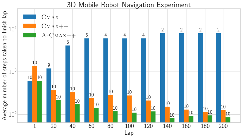
Figure 2: Number of steps taken to finish a lap averaged across 10 instances each with $5$ icy patches placed randomly around the track. The number above each bar reports the number of instances in which the robot was successful in finishing the respective lap within $10000$ time steps.

Since the state space is small, we use Algorithm 2 for Cmax++ and A-Cmax++. For A-Cmax++, we use a non-increasing sequence with $\alpha_{i}=1+\beta_{i}$ where $\beta_{1}=100$ and $\beta_{i}$ is decreased by 2.5 after every $5$ repetitions (See Appendix for more details on choosing the sequence.) We compare both algorithms with Cmax. For all the approaches, we perform $K=100$ expansions. Since the motion primitives are computed offline using an expensive procedure, it is not feasible to update the dynamics of model $\hat{M}$ online and hence, we do not compare with any model learning baselines. We also conducted several experiments with model-free Q-learning, and found that it performed poorly requiring a very large number of executions and finishing only 10 laps in the best case. Hence, we do not include it in our results shown in Figure 2.

Cmax performs well in the early laps computing paths with lower costs compared to Cmax++. However, after a few laps the robot using Cmax gets stuck within an icy patch and does not make any more progress. Observe that when the robot is inside the icy patch, Assumption 4.1 is violated and Cmax ends up inflating all transitions that take the robot out of the patch leading to the robot finishing $200$ laps in $2$ out of $10$ instances. Cmax++, on the other hand, is suboptimal in the initial laps, but converges to paths with lower costs in later laps. More importantly, the robot using Cmax++ manages to finish $200$ laps in all $10$ instances. A-Cmax++ also successfully finishes $200$ laps in all $10$ instances. However, it outperforms both Cmax and Cmax++ in all laps by intelligently switching between them achieving goal-driven behavior in early laps and optimal behavior in later laps. Thus, A-Cmax++ combines the advantages of Cmax and Cmax++.

5.2 7D Pick-and-Place with a Heavy Object

Repetition$\rightarrow$	${1}$		${5}$		${10}$		${15}$		${20}$
	Steps	Success	Steps	Success	Steps	Success	Steps	Success	Steps	Success
Cmax	$\mathbf{17.8\pm 3.4}$	$100\%$	$13.6\pm 0.5$	$60\%$	$18\pm 0$	$20\%$	$15\pm 0$	$20\%$	$15\pm 0$	$20\%$
Cmax++	$\mathbf{17\pm 4.9}$	$100\%$	$14.2\pm 3.3$	$100\%$	$\mathbf{10.6\pm 0.3}$	$100\%$	$\mathbf{11\pm 0}$	$100\%$	$\mathbf{10.8\pm 0.1}$	$100\%$
A-Cmax++	$\mathbf{17.8\pm 3.4}$	$100\%$	$\mathbf{11.6\pm 0.7}$	$100\%$	$17\pm 6$	$100\%$	$\mathbf{10.4\pm 0.3}$	$100\%$	$\mathbf{10.6\pm 0.4}$	$100\%$
Model KNN	$40.6\pm 7.3$	$100\%$	$12.8\pm 1.3$	$100\%$	$29.6\pm 16.1$	$100\%$	$15.8\pm 2.9$	$100\%$	$12.4\pm 1.4$	$100\%$
Model NN	$56\pm 16.2$	$100\%$	$208.2\pm 92.1$	$80\%$	$124.5\pm 81.6$	$40\%$	$28\pm 7.7$	$40\%$	$37.5\pm 20.1$	$40\%$
Q-learning	$172.4\pm 75$	$100\%$	$23.2\pm 10.3$	$80\%$	$26.5\pm 6.7$	$80\%$	$18\pm 2.8$	$80\%$	$10.2\pm 0.6$	$80\%$

Table 1: Number of steps taken to reach the goal in $7$D pick-and-place experiment for $5$ instances, each with random start and obstacle locations. We report mean and standard error only among successful instances in which the robot reached the goal within $500$ timesteps. The success subcolumn indicates percentage of successful instances.

The task in this experiment is to pick and place a heavy object from a shorter table, using a $7$ degree-of-freedom (DOF) robotic arm (Figure 1 left) to a goal pose on a taller table, while avoiding an obstacle. As the object is heavy, the arm cannot generate the required force in certain configurations and can only lift the object to small heights. The problem is represented as planning in $7$D discrete statespace where the first $6$ dimensions describe the $6$ DOF pose of the arm end-effector, and the last dimension corresponds to the redundant DOF in the arm. The action space $\mathbb{A}$ is a discrete set of $14$ actions corresponding to moving in each dimension by a fixed offset in the positive or negative direction. The model $\hat{M}$ used for planning models the object as light, and hence does not capture the dynamics of the arm correctly when it tries to lift the heavy object. The state space is discretized into $10$ cells in each dimension resulting in a total of $10^{7}$ states. Thus, we need to use Algorithm 3 for Cmax++ and A-Cmax++. The goal is to pick and place the object for $20$ repetitions where at the start of each repetition the object is in the start pose and needs to reach the goal pose by the end of repetition.

We compare with Cmax for large state spaces, model-free Q-learning (van Hasselt, Guez, and Silver 2016), and residual model learning baselines (Saveriano et al. 2017). We chose two kinds of function approximators for the learned residual dynamics: global function approximators such as Neural Networks (NN) and local memory-based function approximators such as K-Nearest Neighbors regression (KNN.) Q-learning baseline uses $Q$-values that are cleverly initialized using the model $\hat{M}$ making it a strong model-free baseline. We use the same neural network function approximators for maintaining value estimates for all approaches and perform $K=5$ expansions. We chose the metric $d$ as the manhattan metric and use $\xi=0$ for this experiment. We use a radius of $\delta=3$ for the hyperspheres introduced in the $7$D discrete state space, and to ensure fair comparison use the same radius for KNN regression. These values are chosen to reflect the discrepancies observed when the arm tries to lift the object. All approaches use the same initial value estimates obtained through planning in $\hat{M}$. A-Cmax++ uses a non-increasing sequence $\alpha_{i}=1+\beta_{i}$ where $\beta_{1}=4$ and $\beta_{i+1}=0.5\beta_{i}$.

The results are presented in Table 1. Model-free Q-learning takes a large number of executions in the initial repetitions to estimate accurate $Q$-value estimates but in later repetitions computes paths with lower costs managing to finish all repetitions in $4$ out of $5$ instances. Among the residual model learning baselines, the KNN approximator is successful in all instances but takes a large number of executions to learn the true dynamics, while the NN approximator finishes all repetitions in only $2$ instances. Cmax performs well in the initial repetitions but quickly gets stuck due to inflated costs and manages to complete the task for $20$ repetitions in only $1$ instance. Cmax++ is successful in finishing the task in all instances and repetitions, while improving performance across repetitions. Finally as expected, A-Cmax++ also finishes all repetitions, sometimes even having better performance than Cmax and Cmax++.

6 Discussion and Future Work

A major advantage of Cmax++ is that, unlike previous approaches that deal with inaccurate models, it can exploit inaccurately modeled transitions without wasting online executions to learn the true dynamics. It estimates the $Q$-value of incorrect transitions leveraging past experience and enables the planner to compute solutions containing such transitions. Thus, Cmax++ is especially useful in robotic domains with repetitive tasks where the true dynamics are intractable to model, such as deformable manipulation, or vary over time due to reasons such as wear and tear. Furthermore, the optimistic model assumption is easier to satisfy, when compared to assumptions used by previous approaches like Cmax, and performance of Cmax++ degrades gracefully with the accuracy of the model reducing to Q-learning in the case where the model is inaccurate everywhere. Limitations of Cmax++ and A-Cmax++ include hyperparameters such as the radius $\delta$ and the sequence $\{\alpha_{i}\}$, which might need to be tuned for the task. However, from our sensitivity experiments (see Appendix) we observe that A-Cmax++ performance is robust to the choice of sequence $\{\alpha_{i}\}$ as long as it is non-increasing. Note that Assumption 4.2 can be restrictive for tasks where designing an initial optimistic model requires extensive domain knowledge. However, it is infeasible to relax this assumption further without resorting to global undirected exploration techniques (Thrun 1992), which are highly sample inefficient, to ensure completeness.

An interesting future direction is to interleave model identification with Cmax++ to combine the best of approaches that learn the true dynamics and Cmax++. For instance, given a set of plausible forward models we seek to quickly identify the best model while ensuring efficient performance in each repetition.

Appendix A Sensitivity Experiments

In this section, we present the results of our sensitivity experiments examining the performance of A-Cmax++ with the choice of the sequence $\{\alpha_{i}\}$. We compare the performance of different choices of the sequence $\{\alpha_{i}\}$ on the $3$D mobile robot navigation task. For each run, we average the results across $5$ instances with randomly placed ice patches and present the mean and standard errors. To keep the figures concise, we plot the cumulative number of steps taken to reach the goal from the start of the first lap to the current lap across all laps. In all our runs, A-Cmax++ successfully completes all $200$ laps and hence, we do not report the number of successful instances in our results.

We choose $4$ schedules for the sequence $\{\alpha_{i}\}$:

1. Exponential Schedule: In this schedule, we vary $\beta_{i+1}=\rho\beta_{i}$ where $\rho<1$ is a constant that is tuned and $\alpha_{i}=1+\beta_{i}$. Observe that as $i\rightarrow\infty$, $\alpha_{i}\rightarrow 1$ and that the sequence $\{\alpha_{i}\}$ is a decreasing sequence.

   We vary both the initial $\beta_{1}$ chosen and the constant $\rho$ in our experiments. For $\beta_{1}$ we choose among values $[10,100,1000]$ and $\rho$ is chosen among $[0.5,0.7,0.9]$. The results are shown in Figure 3.

   

   Figure 3: Sensitivity experiments with an exponential schedule

   All choices have almost the same performance with $\beta_{1}=1000$ and $\rho=0.9$ having the best performance initially but has slightly worse performance in the last several laps. The choice of $\beta_{1}=100$ and $\rho=0.9$ seems to be a good choice with great performance in both initial and final laps.

2. Linear Schedule: In this schedule, we vary $\beta_{i+1}=\beta_{i}-\eta$ where $\alpha_{i}=1+\beta_{i}$ and $\eta>0$ is a constant that is determined so that $\beta_{200}=0$, i.e. $\alpha_{200}=1$. Hence, we have $\eta=\frac{\beta_{1}}{200}$.

   We vary the initial $\beta_{1}$ and choose among values $[10,100,200]$. The results are shown in Figure 4.

   

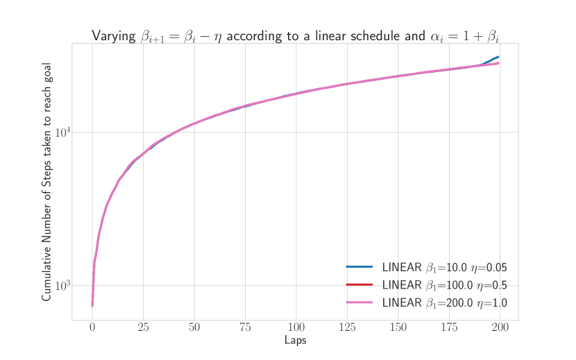
   Figure 4: Sensitivity experiments with a linear schedule

   All three choices have the same performance except in the last few laps where $\beta_{1}=10$ degrades while the other two choices perform well.

3. Time Decay Schedule: In this schedule, we vary $\beta_{i+1}=\frac{\beta_{1}}{i+1}$ where $\alpha_{i}=1+\beta_{i}$. In other words, we decay $\beta$ at the rate of $\frac{1}{i}$ where $i$ is the lap number. Again, observe that as $i\rightarrow\infty$, we have $\alpha_{i}\rightarrow 1$.

   We vary the initial $\beta_{1}$ and choose among values $[10,100,1000]$. The results are shown in Figure 5.

   

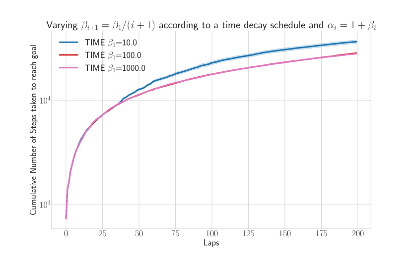
   Figure 5: Sensitivity experiments with a time decay schedule

   The choices of $\beta_{1}=100$ and $\beta_{1}=1000$ have the best (and similar) performance while $\beta_{1}=10$ has a poor performance as it quickly switches to Cmax++ in the early laps and wastes executions learning accurate $Q$-values.

4. Step Schedule: In this schedule, we vary $\beta$ as a step function with $\beta_{i+1}=\beta_{i}-\delta$ if $i$ is a multiple of $\xi$ where $\xi$ is the step frequency, $\alpha_{i}=1+\beta_{i}$ and $\delta$ is a constant that is determined so that $\beta_{200}=0$, i.e. $\alpha_{200}=1$. Hence, we have $\delta=\frac{\beta_{1}\xi}{200}$.

   We vary both the initial $\beta_{1}$ and the step frequency $\xi$. For $\beta_{1}$ we choose among values $[10,100,200]$ and for $\xi$ we choose among $[5,10,20]$. The results are shown in Figure 6.

   

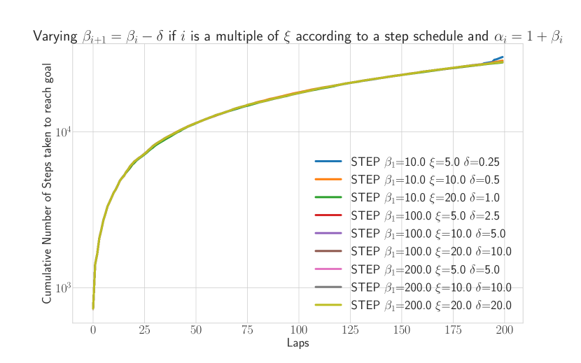
   Figure 6: Sensitivity experiments with a step schedule

   All choices have the same performance and A-Cmax++ seems to be robust to the choice of step size frequency.

For our final comparison, we will pick the best performing choice among all the schedules and compare performance among these selected choices. The results are shown in Figure 7.

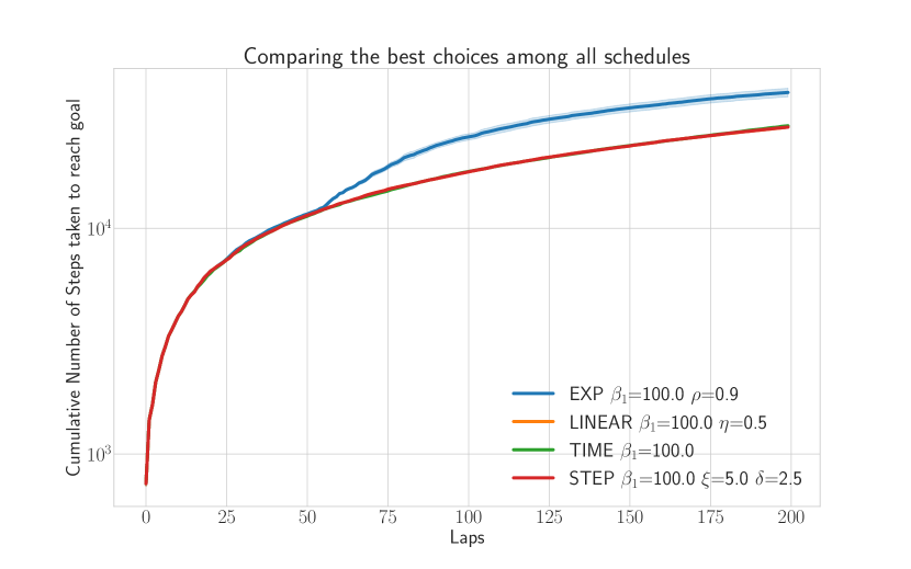
Figure 7: Sensitivity experiments with best choices among all schedules

We can observe that all schedules have the same performance except the exponential schedule which has worse performance. This can be attributed to the rapid decrease in the value of $\beta$ compared to other schedules and thus, around lap $50$ A-Cmax++ switches to Cmax++ resulting in a large number of executions wasted to learn accurate $Q$-value estimates. This does not happen for other schedules as they decrease $\beta$ gradually and thus, spreading out the executions used to learn accurate $Q$-value estimates across several laps and not performing poorly in any single lap.

Appendix B Proofs

In this section, we present the assumptions and proofs that result in the theoretical guarantees of Cmax++ and A-Cmax++.

B.1 Significance of Optimistic Model Assumption

To understand the significance of the optimistic model assumption, it is important to note that completeness guarantees usually require the use of admissible and consistent value estimates, i.e. estimates that always underestimate the true cost-to-goal values. This requirement needs to hold every time we plan (or replan) to ensure that we never discard a path as being expensive in terms of cost, when it is cheap in reality.

All our guarantees assume that the initial value estimates are consistent and admissible, but to ensure that they always remain consistent and admissible throughout execution, we need the optimistic model assumption. This assumption ensures that updating value estimates by planning in the model $\hat{M}$ always results in estimates that are admissible and consistent. In other words, the optimal value function (which we obtain by doing full state space planning in $\hat{M}$) of the model $\hat{M}$ always underestimates the optimal value function of the environment $M$ at all states $s\in\mathbb{S}$.

A very intuitive way to understand the assumption is to imagine a navigation task where the robot is navigating from a start to goal in the presence of obstacles. In this example, the optimistic model assumption requires that the model should never place an obstacle in a location when there isn’t an obstacle in the environment at the same location. However, if there truly is an obstacle at some location, then the model can either have an obstacle or not have one at the same location. Put simply, an agent that is planning using the model should never be “pleasantly surprised” by what it sees in the environment. Several other intuitive examples are presented in (Jiang 2018) and we recommend the reader to look at them for more intuition.

B.2 Completeness Proof

To prove completeness, first we need to note that the $Q$-update in Cmax++ always ensures that the $Q$-value estimates remain consistent and admissible as long as the state value estimates remain consistent and admissible. We have already seen why the optimistic model assumption ensures that the state value estimates always remain consistent and admissible. Thus, we can use Theorem 3 from RTAA* (Koenig and Likhachev 2006) in conjunction with the optimistic model assumption to ensure completeness. Note that if the model is inaccurate everywhere, then our planner reduces to doing $K=1$ expansions at every time step and acts similar to $Q$-learning, which is also guaranteed to be complete with admissible and consistent estimates (Koenig and Simmons 1993). The worst case bound of $|\mathbb{S}|^{3}$ steps is taken directly from the upper bound on $Q$-learning from (Koenig and Simmons 1993). The above arguments are true for both Cmax++ and A-Cmax++. Note that for A-Cmax++ if all paths to the goal contains an incorrect transition then the penalized value estimate $\tilde{V}(s)>\alpha V(s)$ for any finite $\alpha$ and thus, will fall back on Cmax++.

For the second part of the theorem, the assumption of Cmax (we will refer this as optimistic penalized model assumption) in conjunction with RTAA* guarantee again ensures completeness for Cmax++ and A-Cmax++. To see this, observe that the optimistic penalized model assumption ensures that the value estimates are always admissible and consistent w.r.t the true penalized model ($\tilde{M}_{\mathcal{X}}$ where $\mathcal{X}$ contains all the incorrect transitions) and from the assumption, we know that there exists a path to the goal in the true penalized model. Hence, Cmax++ and A-Cmax++ are bound to find this path.

Cmax++ again utilizes the worst case bounds of $Q$-learning under the optimistic penalized assumption as well and attains an upper bound of $|\mathbb{S}|^{3}$ steps. However, A-Cmax++ with a sufficiently large $\alpha_{i}$ for any repetition $i$ acts similar to Cmax, and thereby can utilize the worst case bounds of LRTA* (which is simply RTAA* with $K=1$ expansions) from (Koenig and Simmons 1993) giving an upper bound of $|\mathbb{S}|^{2}$ time steps. This shows the advantage of A-Cmax++ over Cmax++, especially in earlier repetitions when the incorrect set $\mathcal{X}$ is small (thus, making the optimistic penalized model assumption hold,) and $\alpha_{i}$ is large.

B.3 Asymptotic Convergence Proof

The asymptotic convergence proof completely relies on the asymptotic convergence of $Q$-learning (Koenig and Simmons 1993) and asymptotic convergence of LRTA* (Korf 1990) to optimal value estimates. The proof again crucially relies on the fact that the value estimates always remain admissible and consistent, which is ensured by the optimistic model assumption. Note that the optimistic penalized model assumption is not enough to guarantee asymptotic convergence to the optimal cost in $M$ as we penalize incorrect transitions. However, it is possible to show that under the optimistic penalized model assumption both Cmax++ and A-Cmax++ converge to the optimal cost in the true penalized model $\tilde{M}_{\mathcal{X}}$ where $\mathcal{X}$ contains all incorrect transitions.

Appendix C Experiment Details

All experiments were implemented using Python 3.6 and run on a $3.1$GHz Intel Core i$5$ machine. We use PyTorch (Paszke et al. 2019) to train neural network function approximators in our $7$D experiments, and use Box2D (Catto 2007) for our 3D mobile robot simulation (similar to OpenAI Gym (Brockman et al. 2016) car_racing environment) and use PyBullet (Coumans et al. 2013) for our $7$D PR2 experiments.

C.1 3D Mobile Robot Navigation with Icy Patches

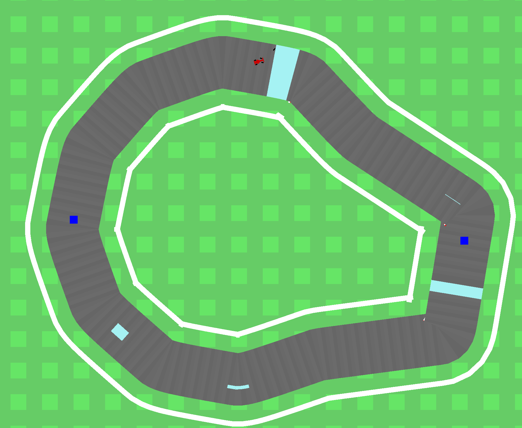
Figure 8: $3$D Mobile Robot experiment example track

An example track used in the $3$D experiment is shown in Figure 8. We generate $66$ motion primitives offline using the following procedure: (a) We first define the primitive action set for the robot by discretizing the steering angle into 3 cells, one corresponding to zero and the other two corresponding to $+0.6$ and $-0.6$ radians. We also discretize the speed of the robot to 2 cells corresponding to $+2$m/s and $-2$m/s, (b) We then discretize the state space into a $100\times 100$ grid in $XY$ space and $16$ cells in $\theta$ dimension. Thus, we have a $100\times 100\times 16$ grid in $XY\theta$ space., (c) We then initialize the robot at $(0,0)$ $xy$ location with different headings chosen among $[0,\cdots,15]$ and roll out all possible sequences of primitive actions for all possible motion primitive lengths from $1$ to $15$ time steps, (d) We filter out all motion primitives whose end point is very close to a cell center in the $XY\theta$ grid. During execution, we use a pure pursuit controller to track the motion primitive so that the robot always starts and ends on a cell center. During planning, we simply use the discrete offsets stored in the motion primitive to compute the next state (and thus, the model dynamics are pre-computed offline during motion primitive generation.)

The cost function used is as follows: for any motion primitive $a$ and state $s$, the cost of executing $a$ from $s$ is given by $c(s,a)=\sum_{s^{\prime}}c^{\prime}(s^{\prime})$ where $c^{\prime}$ is a pre-defined cost map over the $100\times 100\times 16$ grid and $s^{\prime}$ is all the intermediate states (including the final state) that the robot goes through while executing the motion primitive $a$ from $s$. The pre-defined cost map is defined as follows: $c^{\prime}(s)=1$ if state $s$ lies on the track (i.e. $xy$ location corresponding to $s$ lies on the track) and $c^{\prime}(s)=100$ otherwise (i.e. all $xy$ locations corresponding to grass or wall has a cost of $100$). This encourages the planner to come up with a path that lies completely on the track.

We define two checkpoints on the opposite ends of the track (shown as blue squares in Figure 8.) The goal of the robot is to reach the next checkpoint incurring least cost while staying on the track. Note that this requires the robot to complete laps around the track as quickly as possible. Since the state space is small, we maintain value estimates $V,Q,\tilde{V}$ using tables and update the appropriate table entry for each value update. The tables are initialized with value estimates obtained by planning in the model $\hat{M}$ using a planner with $K=100$ expansions until the robot can efficiently complete the laps using the optimal paths. However, this does not mean that the initial value estimates are the optimal values for $\hat{M}$ dynamics since the planner looks ahead and can achieve optimal paths with underestimated value functions. Nevertheless, these estimates are highly informative.

C.2 7D Pick-and-Place with a Heavy Object

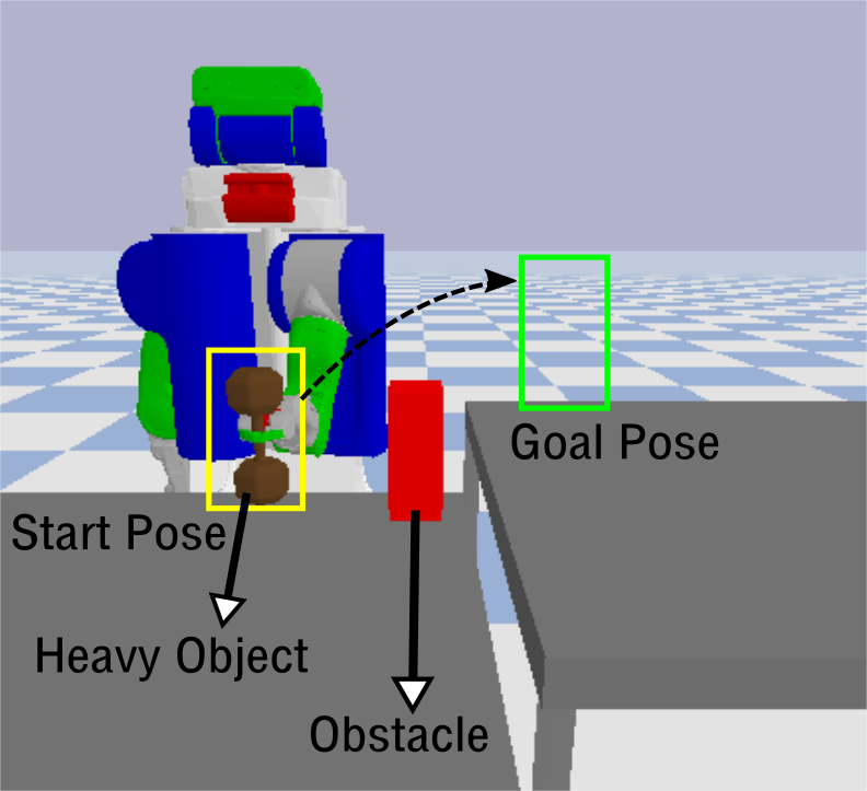
Figure 9: $7$D Pick-and-Place Experiment

For our $7$D experiments, we make use of Bullet Physics Engine through the pyBullet interface. For motion planning and other simulation capabilities we make use of ss-pybullet library (Garrett 2018). The task is shown in Figure 9. The goal is for the robot to pick the heavy object from its start pose and place it at its goal pose while avoiding the obstacle, without any resets. Since the object is heavy, the robot fails to lift the object in certain configurations where it cannot generate the required torque to lift the object. Thus, the robot while lifting the object might fail to reach the goal waypoint and onky reach an intermediate waypoint resulting in discrepancies between modeled and true dynamics.

This is represented as a planning problem in $7$D statespace. The first $6$ dimensions correspond to the $6$DOF pose of the object (or gripper,) and the last dimension corresponds to the redundant DOF in the arm (in our case, it is the upper arm roll joint.) Given a $7$D configuration, we use IKFast library (Diankov 2010) to compute the corresponding $7$D joint angle configuration. The action space consists of $14$ motion primitives that move the arm by a fixed offset in each of the $7$ dimensions in positive and negative directions. The discrepancies in this experiment are only in the $Z$ dimension corresponding to lifting the object. For planning, we simply use a kinematic model of the arm and assume that the object being lifted is extremely light. Thus, we do not need to explicitly consider dynamics during planning. However, during execution we take the dynamics into account by executing the motion primitives in the simulator. The cost of any transition is $1$ if the object is not at goal pose, $0$ if the object is at goal pose. We start the next repetition only if the robot reached the goal pose in the previous repetition.

The $7$D state space is discretized into $10$ cells in each dimension resulting in $10^{7}$ states. Since the state space is large we use neural network function approximators to maintain the value functions $V,Q,\tilde{V}$. For the state value functions $V,\tilde{V}$ we use the following neural network approximator: a feedforward network with $3$ hidden layers consisting of $64$ units each, we use ReLU activations after each layer except the last layer, the network takes as input a $34$D feature representation of the $7$D state computed as follows:

• For any discrete state $s$, we compute a continuous $10$D representation $r(s)$ that is used to construct the features

  • The discrete state is represented as $(xd,yd,zd,rd,pd,yd,rjointd)$ where $(xd,yd,zd)$ represents the $3$D discrete location of the object (or gripper,) $(rd,pd,yd)$ represents the discrete roll, pitch, yaw of the object (or gripper,) and $rjointd$ represents the discrete redundant joint angle

  • We convert $(xd,yd,zd)$ to a continuous representation by simply dividing by the grid size in those dimensions, i.e. $(xc,yc,zc)=(xd/10,yd/10,zd/10)$

  • We do a similar construction for $rjointc$, i.e. $rjointc=rjointd/10$

  • However, note that $rd,pd,yd$ are angular dimensions and simply dividing by grid size would not encode the wrap around nature that is inherent in angular dimensions (we did not have this problem for $rjointd$ as the redundant joint angle has lower and upper limits, and is always recorded as a value between those limits.) To account for this, we use a sine-cosine representation defined as $(rc1,rc2,pc1,pc2.yc1,yc2)=(sin(rc),cos(rc),sin(pc),cos(pc),sin(yc),cos(yc))$ where $rc,pc,yc$ are the roll, pitch, yaw angles corresponding to the cell centers of the grid cells $rd,pd,yd$.

  • Thus, the final $10$D representation of state $s$ is given by $r(s)=(xc,yc,zc,rc1,rc2,pc1,pc2,yc1,yc2,rjointc)$

  • We also define a truncated $9$D representation $r^{\prime}(s)=(xc,yc,zc,rc1,rc2,pc1,pc2,yc1,yc2)$ and a $3$D representation $r^{\prime\prime}(s)=(xc,yc,zc)$

• The first feature is the $9$D relative position of the $6$D goal pose w.r.t the object $f1=r^{\prime}(g)-r^{\prime}(s)$

• The second feature is the $10$D relative position of the object w.r.t the gripper home state $h$, $f2=r(s)-r(h)$

• The third feature is the $9$D relative position of the goal w.r.t the gripper home state $h$, $f3=r^{\prime}(g)-r^{\prime}(h)$

• The fourth feature is the $3$D relative position of the obstacle left top corner $o1$ w.r.t the object, $f4=r^{\prime\prime}(o1)-r^{\prime\prime}(s)$

• The fifth and final feature is the $3$D relative position of the object right bottom corner $o2$ w.r.t. the object, $f5=r^{\prime\prime}(o2)-r^{\prime\prime}(s)$

• Thus, the final $34$D feature representation is given by $f(s)=(f1,f2,f3,f4,f5)$.

The output of the network is a single scalar value representing the cost-to-goal of the input state. Instead of learning the cost-to-goal/value from scratch, we start with an initial value estimate that is hardcoded (manhattan distance to goal in the $7$D discrete grid) and the neural network approximator is used to learn a residual on top of it. A similar trick was used in Cmax (Vemula et al. 2020). The residual state value function approximator was initialized to output $0$ for all $s\in\mathbb{S}$. We use a similar architecture for the residual $Q$-value function approximator but it takes as input the $34$D state feature representation and outputs a vector in $\mathbb{R}^{|\mathbb{A}|}$ (in our case, $\mathbb{R}^{14}$) to represent the cost-to-goal estimate for each action $a\in\mathbb{A}$. We also use the same hardcoded value estimates as before in addition to the residual approximator to construct the $Q$-values. All baselines and proposed approaches use the same function approximator and same initial hardcoded value estimates to ensure fair comparison. The value function approximators are trained using mean squared loss.

The residual model learning baseline with neural network (NN) function approximator uses the following architecture: $2$ hidden layers each with $64$ units and all layers are followed by ReLU activations except the last layer. The input of the network is the $34$D feature representation of the state and a one-hot encoding of the action in $\mathbb{R}^{1}4$. The output of the network is the $7$D continuous state which is added to the state predicted by the model $\hat{M}$. The loss function used to train the network is a simple mean squared loss. The residual model learning baseline with K-Nearest Neighbor regression approximator (KNN) uses a manhattan radius of $3$ in the discrete $7$D state space. We compute the prediction by averaging the next state residual vector observed in the past for any state that lies within the radius of the current state. The averaged residual is added to the next state predicted by model $\hat{M}$ to obtain the learned next state.

We use Adam optimizer (Kingma and Ba 2015) with a learning rate of $0.001$ and a weight decay (L$2$ regularization coefficient) of $0.001$ to train all the neural network function approximators in all approaches. We use a batch size of $32$ for the state value function approximators and a batch size of $128$ for the $Q$-value function approximators. We perform $U=3$ updates for state value function and $U=5$ updates for state-action value function for each time step. We update the parameters of all neural network approximators using a polyak averaging coefficient of $0.5$.

Finally, we use hindsight experience replay trick (Andrychowicz et al. 2017) in training all the value function approximators with the probability of sampling any future state in past trajectories as the goal set to $0.7$. This is crucial as our cost function used is extremely sparse.

References

- Abbeel, Quigley, and Ng (2006) Abbeel, P.; Quigley, M.; and Ng, A. Y. 2006. Using inaccurate models in reinforcement learning. In Cohen, W. W.; and Moore, A. W., eds., Machine Learning, Proceedings of the Twenty-Third International Conference (ICML 2006), Pittsburgh, Pennsylvania, USA, June 25-29, 2006, volume 148 of ACM International Conference Proceeding Series, 1–8. ACM. doi:10.1145/1143844.1143845. URL https://doi.org/10.1145/1143844.1143845.
- Andrychowicz et al. (2017) Andrychowicz, M.; Crow, D.; Ray, A.; Schneider, J.; Fong, R.; Welinder, P.; McGrew, B.; Tobin, J.; Abbeel, P.; and Zaremba, W. 2017. Hindsight Experience Replay. In Guyon, I.; von Luxburg, U.; Bengio, S.; Wallach, H. M.; Fergus, R.; Vishwanathan, S. V. N.; and Garnett, R., eds., Advances in Neural Information Processing Systems 30: Annual Conference on Neural Information Processing Systems 2017, 4-9 December 2017, Long Beach, CA, USA, 5048–5058. URL http://papers.nips.cc/paper/7090-hindsight-experience-replay.
- Berenson, Abbeel, and Goldberg (2012) Berenson, D.; Abbeel, P.; and Goldberg, K. 2012. A robot path planning framework that learns from experience. In IEEE International Conference on Robotics and Automation, ICRA 2012, 14-18 May, 2012, St. Paul, Minnesota, USA, 3671–3678. IEEE. doi:10.1109/ICRA.2012.6224742. URL https://doi.org/10.1109/ICRA.2012.6224742.
- Bertsekas (2005) Bertsekas, D. P. 2005. Dynamic programming and optimal control, 3rd Edition. Athena Scientific. ISBN 1886529264. URL https://www.worldcat.org/oclc/314894080.
- Brockman et al. (2016) Brockman, G.; Cheung, V.; Pettersson, L.; Schneider, J.; Schulman, J.; Tang, J.; and Zaremba, W. 2016. OpenAI Gym.
- Catto (2007) Catto, E. 2007. Box2d physics engine.
- Coumans et al. (2013) Coumans, E.; et al. 2013. Bullet physics library. Open source: bulletphysics. org 15(49): 5.
- Diankov (2010) Diankov, R. 2010. Automated Construction of Robotic Manipulation Programs. Ph.D. thesis, Carnegie Mellon University, Robotics Institute. URL http://www.programmingvision.com/rosen˙diankov˙thesis.pdf.
- Essahbi, Bouzgarrou, and Gogu (2012) Essahbi, N.; Bouzgarrou, B. C.; and Gogu, G. 2012. Soft Material Modeling for Robotic Manipulation. In Mechanisms, Mechanical Transmissions and Robotics, volume 162 of Applied Mechanics and Materials, 184–193. Trans Tech Publications Ltd. doi:10.4028/www.scientific.net/AMM.162.184.
- Garrett (2018) Garrett, C. R. 2018. ss-pybullet library. URL https://github.com/caelan/ss-pybullet.
- Hauser et al. (2006) Hauser, K. K.; Bretl, T.; Harada, K.; and Latombe, J. 2006. Using Motion Primitives in Probabilistic Sample-Based Planning for Humanoid Robots. In Akella, S.; Amato, N. M.; Huang, W. H.; and Mishra, B., eds., Algorithmic Foundation of Robotics VII, Selected Contributions of the Seventh International Workshop on the Algorithmic Foundations of Robotics, WAFR 2006, July 16-18, 2006, New York, NY, USA, volume 47 of Springer Tracts in Advanced Robotics, 507–522. Springer. doi:10.1007/978-3-540-68405-3“˙32. URL https://doi.org/10.1007/978-3-540-68405-3“˙32.
- Ji and Xiao (2001) Ji, X.; and Xiao, J. 2001. Planning Motions Compliant to Complex Contact States. IJ Robotics Res. 20(6): 446–465. doi:10.1177/02783640122067480. URL https://doi.org/10.1177/02783640122067480.
- Jiang (2018) Jiang, N. 2018. PAC Reinforcement Learning With an Imperfect Model. In McIlraith, S. A.; and Weinberger, K. Q., eds., Proceedings of the Thirty-Second AAAI Conference on Artificial Intelligence, (AAAI-18), the 30th innovative Applications of Artificial Intelligence (IAAI-18), and the 8th AAAI Symposium on Educational Advances in Artificial Intelligence (EAAI-18), New Orleans, Louisiana, USA, February 2-7, 2018, 3334–3341. AAAI Press. URL https://www.aaai.org/ocs/index.php/AAAI/AAAI18/paper/view/16052.
- Kingma and Ba (2015) Kingma, D. P.; and Ba, J. 2015. Adam: A Method for Stochastic Optimization. In Bengio, Y.; and LeCun, Y., eds., 3rd International Conference on Learning Representations, ICLR 2015, San Diego, CA, USA, May 7-9, 2015, Conference Track Proceedings. URL http://arxiv.org/abs/1412.6980.
- Koenig and Likhachev (2006) Koenig, S.; and Likhachev, M. 2006. Real-time adaptive A*. In Nakashima, H.; Wellman, M. P.; Weiss, G.; and Stone, P., eds., 5th International Joint Conference on Autonomous Agents and Multiagent Systems (AAMAS 2006), Hakodate, Japan, May 8-12, 2006, 281–288. ACM. doi:10.1145/1160633.1160682. URL https://doi.org/10.1145/1160633.1160682.
- Koenig and Simmons (1993) Koenig, S.; and Simmons, R. G. 1993. Complexity Analysis of Real-Time Reinforcement Learning. In Fikes, R.; and Lehnert, W. G., eds., Proceedings of the 11th National Conference on Artificial Intelligence. Washington, DC, USA, July 11-15, 1993, 99–107. AAAI Press / The MIT Press. URL http://www.aaai.org/Library/AAAI/1993/aaai93-016.php.
- Korf (1990) Korf, R. E. 1990. Real-Time Heuristic Search. Artif. Intell. 42(2-3): 189–211. doi:10.1016/0004-3702(90)90054-4. URL https://doi.org/10.1016/0004-3702(90)90054-4.
- Lagrassa, Lee, and Kroemer (2020) Lagrassa, A.; Lee, S.; and Kroemer, O. 2020. Learning skills to patch plans based on inaccurate models. In 2020 IEEE International Conference on Intelligent Robots and Systems (IROS).
- Lee et al. (2020) Lee, M. A.; Florensa, C.; Tremblay, J.; Ratliff, N. D.; Garg, A.; Ramos, F.; and Fox, D. 2020. Guided Uncertainty-Aware Policy Optimization: Combining Learning and Model-Based Strategies for Sample-Efficient Policy Learning. CoRR abs/2005.10872. URL https://arxiv.org/abs/2005.10872.
- McConachie et al. (2020) McConachie, D.; Power, T.; Mitrano, P.; and Berenson, D. 2020. Learning When to Trust a Dynamics Model for Planning in Reduced State Spaces. IEEE Robotics Autom. Lett. 5(2): 3540–3547. doi:10.1109/LRA.2020.2972858. URL https://doi.org/10.1109/LRA.2020.2972858.
- Paszke et al. (2019) Paszke, A.; Gross, S.; Massa, F.; Lerer, A.; Bradbury, J.; Chanan, G.; Killeen, T.; Lin, Z.; Gimelshein, N.; Antiga, L.; Desmaison, A.; Kopf, A.; Yang, E.; DeVito, Z.; Raison, M.; Tejani, A.; Chilamkurthy, S.; Steiner, B.; Fang, L.; Bai, J.; and Chintala, S. 2019. PyTorch: An Imperative Style, High-Performance Deep Learning Library. In Advances in Neural Information Processing Systems 32, 8024–8035. Curran Associates, Inc. URL http://papers.neurips.cc/paper/9015-pytorch-an-imperative-style-high-performance-deep-learning-library.pdf.
- Pivtoraiko, Knepper, and Kelly (2009) Pivtoraiko, M.; Knepper, R. A.; and Kelly, A. 2009. Differentially constrained mobile robot motion planning in state lattices. J. Field Robotics 26(3): 308–333. doi:10.1002/rob.20285. URL https://doi.org/10.1002/rob.20285.
- Reeds and Shepp (1990) Reeds, J. A.; and Shepp, L. A. 1990. Optimal paths for a car that goes both forwards and backwards. Pacific J. Math. 145(2): 367–393. URL https://projecteuclid.org:443/euclid.pjm/1102645450.
- Saveriano et al. (2017) Saveriano, M.; Yin, Y.; Falco, P.; and Lee, D. 2017. Data-efficient control policy search using residual dynamics learning. In 2017 IEEE/RSJ International Conference on Intelligent Robots and Systems, IROS 2017, Vancouver, BC, Canada, September 24-28, 2017, 4709–4715. IEEE. doi:10.1109/IROS.2017.8206343. URL https://doi.org/10.1109/IROS.2017.8206343.
- Sun et al. (2019) Sun, W.; Jiang, N.; Krishnamurthy, A.; Agarwal, A.; and Langford, J. 2019. Model-based RL in Contextual Decision Processes: PAC bounds and Exponential Improvements over Model-free Approaches. In Beygelzimer, A.; and Hsu, D., eds., Conference on Learning Theory, COLT 2019, 25-28 June 2019, Phoenix, AZ, USA, volume 99 of Proceedings of Machine Learning Research, 2898–2933. PMLR. URL http://proceedings.mlr.press/v99/sun19a.html.
- Sutton (1991) Sutton, R. S. 1991. Dyna, an Integrated Architecture for Learning, Planning, and Reacting. SIGART Bull. 2(4): 160–163. doi:10.1145/122344.122377. URL https://doi.org/10.1145/122344.122377.
- Thrun (1992) Thrun, S. 1992. Efficient Exploration In Reinforcement Learning. Technical Report CMU-CS-92-102, Carnegie Mellon University, Pittsburgh, PA.
- Todorov, Erez, and Tassa (2012) Todorov, E.; Erez, T.; and Tassa, Y. 2012. MuJoCo: A physics engine for model-based control. In 2012 IEEE/RSJ International Conference on Intelligent Robots and Systems, IROS 2012, Vilamoura, Algarve, Portugal, October 7-12, 2012, 5026–5033. IEEE. doi:10.1109/IROS.2012.6386109. URL https://doi.org/10.1109/IROS.2012.6386109.
- van Hasselt, Guez, and Silver (2016) van Hasselt, H.; Guez, A.; and Silver, D. 2016. Deep Reinforcement Learning with Double Q-Learning. In Schuurmans, D.; and Wellman, M. P., eds., Proceedings of the Thirtieth AAAI Conference on Artificial Intelligence, February 12-17, 2016, Phoenix, Arizona, USA, 2094–2100. AAAI Press. URL http://www.aaai.org/ocs/index.php/AAAI/AAAI16/paper/view/12389.
- Vemula et al. (2020) Vemula, A.; Oza, Y.; Bagnell, J.; and Likhachev, M. 2020. Planning and Execution using Inaccurate Models with Provable Guarantees. In Proceedings of Robotics: Science and Systems. Corvalis, Oregon, USA. doi:10.15607/RSS.2020.XVI.001.