AOBTM: Adaptive Online Biterm Topic Modeling for Version Sensitive Short-texts Analysis

Abstract

Analysis of mobile app reviews has shown its important role in requirement engineering, software maintenance and evolution of mobile apps. Mobile app developers check their users’ reviews frequently to clarify the issues experienced by users or capture the new issues that are introduced due to a recent app update. App reviews have a dynamic nature and their discussed topics change over time. The changes in the topics among collected reviews for different versions of an app can reveal important issues about the app update. A main technique in this analysis is using topic modeling algorithms. However, app reviews are short texts and it is challenging to unveil their latent topics over time. Conventional topic models such as Latent Dirichlet Allocation (LDA) and Probabilistic Latent Semantic Analysis (PLSA) suffer from the sparsity of word co-occurrence patterns while inferring topics for short texts. Furthermore, these algorithms cannot capture topics over numerous consecutive time-slices (or versions). Online topic modeling algorithms such as Online LDA (OLDA) and Online Biterm Topic Model (OBTM) speed up the inference of topic models for the texts collected in the latest time-slice by saving a fraction of data from the previous time-slice. But these algorithms do not analyze the statistical-data (such as topic distributions) of all the previous time-slices, which can confer contributions to the topic distribution of the current time-slice.

In this paper, we propose Adaptive Online Biterm Topic Model (AOBTM) to model topics in short texts adaptively. AOBTM alleviates the sparsity problem in short-texts and considers the statistical-data for an optimal number of previous time-slices. We also propose parallel algorithms to automatically determine the optimal number of topics and the best number of previous versions that should be considered in topic inference phase. Automatic evaluation on collections of app reviews and real-world short text datasets confirm that AOBTM can find more coherent topics and outperforms the state-of-the-art baselines. For reproducibility of the results, we open source all scripts.

I Introduction

Mobile app reviews form a main feedback channel for the app developers [1] to evaluate their products and improve application maintenance and evolution tasks [2]. The app developers require to analyze app reviews in order to gain insights about the current state of their apps from users’ perspectives. Mobile app reviews form a feedback channel for the developers [1] to evaluate their products and improve application maintenance and evolution tasks [2]. The app developers must analyze app reviews in order to gain insights about the current state of their apps from users’ perspectives. Several studies have been proposed to analyze the app reviews, including extracting informative text [3], summarizing user reviews [4], identifying the bugs or feature requests [5, 6, 7], prioritizing feature inclusions [8], and extracting insights about the apps [1]. Although the (popular) apps are updated frequently [9], the app review analysis studies mostly consider the app reviews static [10, 11]. However, app reviews have a dynamic nature and their discussed topics change over time. If the update-centric analysis is neglected, it misses the point that feedback are written on a certain update [11]. The change in the topics extracted from reviews for different app versions can reveal important issues about the app [10, 11].

A recent example of the importance of discussed topics over time is the Zoom Cloud Meeting, a popular app for video conferencing. Zoom received massive one-star ratings (the lowest rating) in Google Play Store during the COVID-19 outbreak in March 2020. Most of the issues were related to users’ concerns about data-privacy and security-malpractices. These issues were so severe that in a letter to Zoom, the New York attorney general’s office expressed concerns and addressed security flaws [12]. These issues were extensively discussed in the user reviews and could have been flushed out months ago through proper inspection of the user reviews and topic changes from user feedbacks on Google Play Store.

App reviews are short texts that are time/version sensitive as these texts are generated constantly and are collected regularly for consecutive app versions [10, 9]. The underlying latent topics derived from app reviews can benefit the developers extensively [13]. However, extracting relevant topics from app reviews is challenging due to their dynamic nature and lack of rich context in short texts.

The most popular topic modeling methods for discovering the underlying topics from text-corpus are LDA [14] and PLSA [15]. But these topic models do not perform well with text-corpus containing short-texts as documents [16]. These algorithms consider individual short texts as separate documents and model each of these documents as a mixture of topics, where each topic is considered as a probability distribution over words. The models then utilize various statistical techniques to determine the topic components and mixture coefficients of each document by implicitly capturing the document-level word co-occurrence patterns [17, 18]. While dealing with the typical lengthy documents, the mentioned algorithms could rely on larger word counts to know how the words are related. However, the natural sparseness of the word co-occurrence patterns in each short document makes these models suffer from the data-sparsity problem [19]. Moreover, short texts lack the richness of context, making it more difficult for these topic models to identify the senses of ambiguous words in short documents. Biterm Topic Model (BTM) alleviates these problems by learning topics over short texts and explicitly modeling the generation of biterms in the whole corpus to enhance topic learning [16].

As mentioned, app reviews are usually collected in batches of consecutive time-slices [10]. Each time a new batch of text-data arrives, these topic models (e.g. LDA, BTM) require retraining to discover latent topic distributions from the new dataset, which is prohibitively time and memory consuming. The popular way to alleviate the scalability problem is to develop online algorithms such as Online LDA (OLDA) [20] and Online BTM (OBTM) [16]. These online algorithms store a small fraction of data on the fly in order to accommodate the dataset of the upcoming time-slice. When a new batch of text-data arrives, online algorithms model the topics of texts either by using the statistics of samples collected in the immediately previous version/time-slice [21] or by naively aggregating statistics of all the previous time-slices [16]. However, these online algorithms do not take different versions’ varying contributions into account. Statistics of the textual data collected over different time periods or different versions may have a non-negligible difference in similarity with that of the latest time-slice; and thus, can contribute differently to the latest version[18, 10]. Adaptive versions of online algorithms, such as Adaptively Online LDA (AOLDA), can be used to address the problem of the varying contribution of different versions [10]. But, the underlying model in AOLDA is LDA, which again makes it suffer from the mentioned data-sparsity problem while working with short-texts.

In this paper, we propose a new adaptive online topic model for short texts which takes previous versions’ varying contribution into account. We refer to this novel model as the Adaptive Online Biterm Topic Model (AOBTM). AOBTM inherits the characteristics of BTM to deal with the data sparsity issue. It is an online algorithm that can scale for the increasing volume of the dataset that is generated frequently. AOBTM also endows the statistics of the previous versions with different contributions to the topic distributions of the current version of the dataset. Also, we have employed a preprocessing technique that is useful for yielding better top contributing key-terms to help the manual investigation of the inferred topics. Our contributions are enlisted below:

1. We propose a novel method called AOBTM for version sensitive content analysis for short texts. This method adaptively combines the topic distributions of a selected number prior versions to generate topic distributions of the current version.

2. We propose two parallel algorithms; the first algorithm can identify an optimal number of topics to be derived in the latest version, and the second algorithm can identify the optimal number of previous versions to be taken into consideration for adaptive aggregation of statistical data.

3. To encourage replicability, of the research results, we make all scripts, codes, and graphs available to the community.

We have conducted experiments on app review datasets and Twitter dataset with large number of records to evaluate performance of AOBTM compared to five baseline algorithms. Also, we integrated AOBTM into the state of the art online app-review analysis framework called IDEA for comparison [10]. Our results show that topics captured by AOBTM are more coherent compared to the topics extracted by baseline methods.

The rest of the paper is organized as follows: Section II and III describe the background and our Topic Model Design. Sections IV and V are dedicated to the proposed parallel algorithms and experiments and results, followed by the related works in Section VI. We add threats to validity in section VII and conclude the paper in Section VIII.

II Background and Motivation

II-A Topic Modeling for conventional text-documents

Topic modeling algorithms such as PLSA and LDA are widely embraced for identifying latent semantic structures from text corpus without requiring any prior annotations of the documents [22]. These algorithms observe each document as a mixture of topics while a distribution over the vocabulary terms characterizes each topic. Statistical techniques such as Variational methods and Gibbs sampling are then applied to infer the latent topic distributions of given documents and the word distributions of inferred topics [23]. Although these algorithms and their variants contributed largely in modeling text collections such as blogs, research papers, and news articles [20, 24, 25], these topic models endure considerable performance deterioration while handling short texts [26, 16]. Directly applying these models on short texts suffer from severe data sparsity problem [19] as the frequency of words in the short texts play less discriminative role, which makes it hard to infer words correlation from short documents [19]. The limited contexts in the short text also make it challenging to identify the sense of ambiguous words.

II-B Topic Modeling for short text-documents

Researchers have proposed the numerous topic modeling algorithms for short texts by trying to solve one or two of the following inherent characteristics of the short texts: i) lack of enough word co-occurrence information, probability of most individual short texts being generated by singular topic, ii) inability to fully capture semantically co-related but rarely co-occurring words (due to lack of statistical information of words among texts), and iii) the probability that a single-topic assumption is too strong for some short texts [22]. In [22], Qiang et al. divided the short text topic modeling algorithms into three major categories: Dirichlet multinomial mixture (DMM) based methods, Global word co-occurrences based methods, and Self-aggregation based methods. Brief introductions to the related works can be found in section VI.

II-C Online Topic Modeling for short texts

A particular issue with the traditional topic modeling algorithms is that they can not scale with the expanding dataset. Whenever a new batch of data arrives, these topic models (i.e., LDA, PLSA) need to train from scratch. Moreover, these conventional topic models can not guarantee consistency in the sequence of topics if independent training is performed on different batches of the same corpus [14, 16]. This inconsistency occurs because, before each of the independent training, we set the prior topic distribution to a default value, a Dirichlet parameter; so, the fixed number of topics (assume, $K$) can be generated in any sequence. [16]. For example, when we train a corpus, using BTM or LDA, with $K$ number of topics, each independent training of BTM generates $K$ number of topic distributions, where we can not ascertain that each time we train the corpus, a topic no. $K=k$ (here, $k=[1,...,K]$) will always correspond to a specific topic (i.e., ”UI_component”).

Researchers proposed online models (i.e., OBTM, OLDA) to circumvent the problems with streaming datasets. Here, we can assume that the documents would be generated in streams and can be collected from, divided different time-slices or versions, where the documents are exchangeable in a time-slice. For example, Online BTM (OBTM) accommodates and deals with batches of short-text documents divided into different time-slices or versions. Let’s assume that OBTM has already got the topic distribution for $(t-1)$-th time-slice. When a new batch ($t$-th time-slice) arrives, OBTM utilizes the topic distribution of $(t-1)$-th time-slice to set the prior topic distribution of $t$-th time-slice. It, in turn, ensures that after the training of the $t$-th time-slice, the $k$-th topic in the $t$-th time-slice is closely related to the $k$-th topic generated in the $(t-1)$-th time-slice. If we introduce a completely new topic in the latest batch of documents ($t$-th time-slice), the new topic will merge into one (or more) existing topic(s) generated in the $(t-1)$-th time-slice that has (/have) strong correlation(s) with the introduced topic. [16]

II-D Adaptively Online Topic Modeling for short texts

The problem with online topic modeling algorithms is that they do not consider or compare the varying consequential correlation among all the preceding time slices or versions of the short texts while inferring topics for the latest time-slice. For example, in OBTM, this limitation transpires as the topic model generates the topic distribution of a time-slice by making it directly dependent on the topic distribution of preceding time-slices. If new topics are being introduced in each time-slice, the $k$-th topic in the latest time slice would be significantly different than that of the first time-slice. We can not reliably compare the distribution of the $K=k$-th topic between two non-consecutive time-slices as OBTM does not impose or investigate the varying correlation between them.

In our proposed method, we aim to alleviate the mentioned problem by adaptively integrating the topic distributions of all the previous time-slices with their respective weights as contributions, for generating the prior distribution of the latest, $t$-th time-slice. This way, we can warrant both coherence of specific topics and consistency in the topics’ sequence in all the available versions. The adaptiveness enables us to compare topic distributions of any two different time-slices reliably.

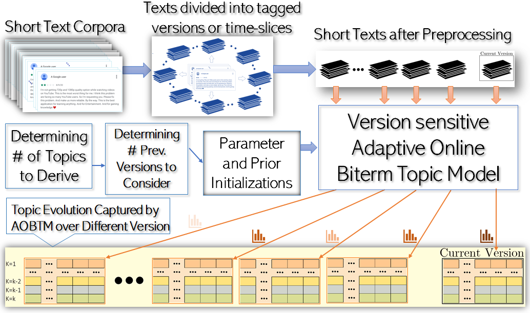
Figure 1: Overview of the Framework

In Figure 1, we show an overview of the framework. Here, version tagged short-texts are processed and fed into the AOBTM algorithm to find better topic distribution for the latest version by leveraging previous versions’ statistical data. The details of each part are discussed in Sections III, IV.

III Adaptive Online Biterm Topic Model

In this section, we discuss the details of the Adaptive Online Biterm Topic Model (AOBTM). This method introduces Adaptiveness to give the online algorithm, OBTM, a version or time-slice sensitivity so that the prior topic distribution of the latest time-slice takes varying contributions (topic distribution-wise) of the previous time-slices into account. After setting the prior, we train the model to find out the final topic distribution. The details of the proposed method are described below.

III-A Applied Biterm Extraction technique

We have adopted the definition of Biterm from [16], where it denotes an unordered term-pair co-occurring in a small, fixed-size window over a term sequence. The fixed-sized window is referred to as short-context. The optimal size of short-context varies from dataset to dataset and can be considered as an important parameter setting. In a given short-context, an unordered pair of any two distinct terms can form a biterm. For example, a short context with size=3, generates the following biterms: $(w_{1},w_{2},w_{3})\Rightarrow\{(w_{1},w_{2}),(w_{2},w_{3}),(w_{1},w_{3})\}$

In previous works of topic labeling (i.e., [27, 28]), inferred topics have been labeled with the term(s), which has(/have) a more significant contribution to the respective topics. Here, term denotes any non-redundant word in the document, which cannot be found in Natural Language Toolkit’s (NLTK) stop-word list. But Gao et al. [9], showed that the most contributing singular term or their combination could not adequately represent the respective topic. So, instead of using singular terms, we use meaningful phrases to label the topics, where a Phrase refers to two frequently co-occurring words. To ensure the comprehensibility of the extracted phrases, we use a Pointwise Mutual Information (PMI)- based phrase extraction method [29], where the higher frequency of two words’ co-occurrence warrants the generation of a more meaningful phrase. For our model, we have empirically set our frequency threshold to 24. After identifying the phrases, we convert them into single terms using ‘_’ (i.e., $w_{1}\_w_{2}$), to train them along with other terms using our algorithm. During biterms extraction, words constructing the phrases are also considered as term when they appear outside identified phrases. We train the phrases to capture their underlying semantics, which, in turn, would help us to label the topics with the most relevant phrases. We will further demonstrate this modification’s impact in the experiment section.

III-B Model Description

To alleviate the data-sparsity problem faced by AOLDA and to capture more coherent, comprehensible, and discriminative topics, we propose an adaptive online topic modeling method, AOBTM, which improves OBTM by adaptively combining the topic distributions in previous versions. The details of the proposed AOBTM method are described in figure 2.

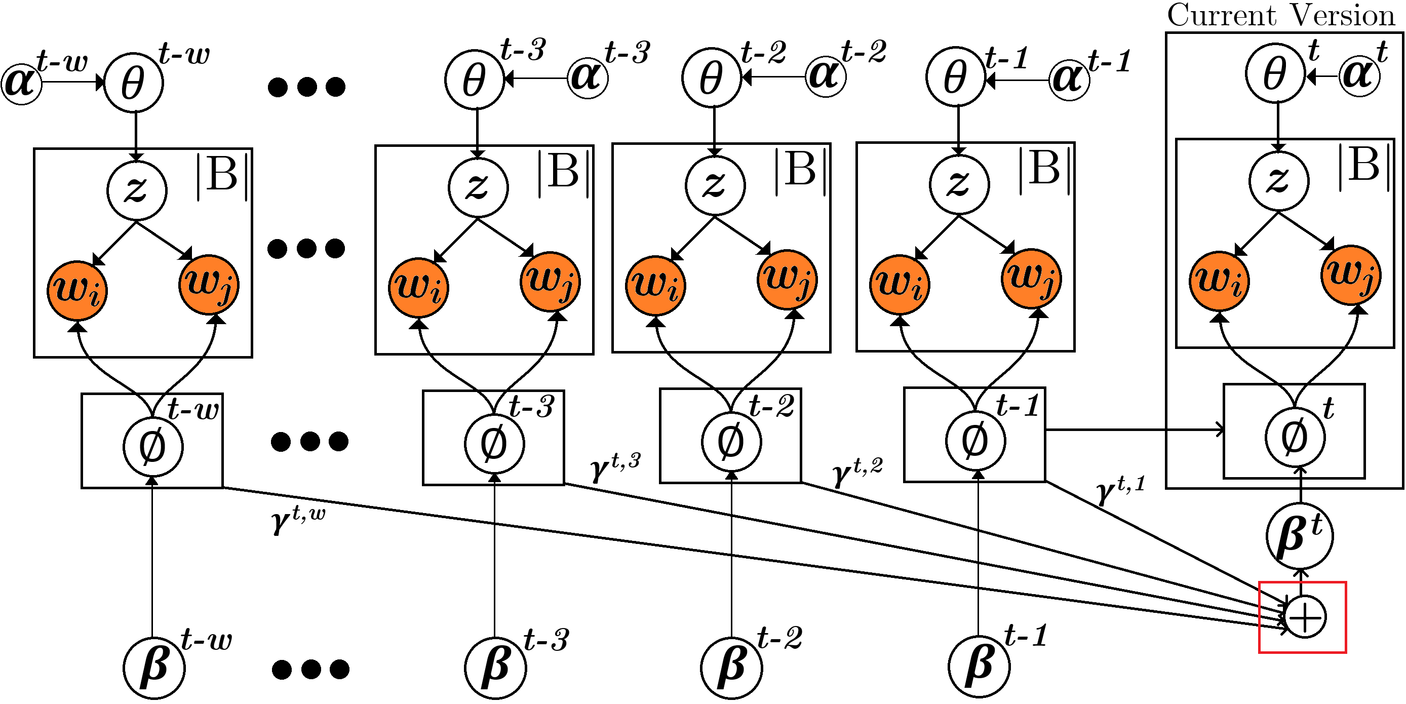
Figure 2: Overview of AOBTM. The red rectangle highlights the adaptive integration of the topics of the w previous versions for generating the prior $\Phi$ in the t-th version

After the preprocessing, the short texts are separated into different time-slices or versions, and input into AOBTM sequentially. AOBTM treats the short texts-set from each time-slice as a separate corpus. We denote the whole corpus as $R$ = $R^{1}$, $R^{2}$, …, $R^{t}$, where t indicates the t-th time-slice. Following the literature, we denote the prior distributions over corpus-topic as $\alpha$ and the prior distributions over topic-words as $\beta$; both $\alpha$ and $\beta$ are defined initially. The topic-word distributions determine the topic’s distribution over all the non-redundant terms (including the phrases) that appear in the corpus. The number of the topics is specified as K. For the k-th topic, $\Phi_{k}^{t}$ is the probability distribution vector over all the input terms in the $t$-th time slice. We introduce a new parameter- $win$ (window size), which defines the number of previous versions to be considered for inferring the topic distributions of the current version. The overview of the AOBTM model is depicted in Figure 2. Different from OBTM (and similar to AOLDA), as Figure 2 shown, we adaptively integrate the topic distributions of the previous $win$ versions, denoted as $\Phi^{t-1},\Phi^{t-2},...,\Phi^{t-i},...,\Phi^{t-win}$, for generating the prior, $\beta^{t}$ for the t-th version. The adaptive integration sums up the topic distributions of different versions with different weights, $\gamma^{t,i}$:

Here, $i$ denotes the $i$-th previous version ($1\leq i\leq w$). $n_{w|k}^{t}$ denotes the number of times word, w is assigned to topic k in time-slice t. The weight $\gamma_{k}^{t,i}$ is determined by considering the similarity of the k-th topic between the (t-i)th version and the (t-1)th version, which is calculated by the following softmax function:

Input : $K,win,\alpha,\beta,\mathbf{B^{(1)},....,\mathbf{B^{(T)}}}$

Output : {$\Phi^{(t)},\theta^{(t)}\}_{t=1}^{T}$

1 Set $\alpha^{(1)}=(\alpha,....,\alpha)$ and $\{\beta_{k}^{(1)}=(\beta,....,\beta)\}_{k=1}^{K}$

2 for $t\leftarrow 1$ to $T$ do

3      Randomly assign topics to biterms in $B^{(t)}$;

4       for $iter\leftarrow 1$ to $N_{iter}$ do

5            foreach biterm $b_{i}=(w_{i,1},w_{i,2})\in B^{(t)}$ do

6                  Draw topic k from Eq. 3;

7                   Update $n_{k}^{(t)},{n_{w_{i,1}}}_{|k}^{(t)}$, and ${n_{w_{i,2}}}_{|k}^{(t)}$;

8                  

9             end foreach

10            Set $\alpha^{(t+1)}$ by Eq.4;

11             Set $\{\beta_{k}^{(t+1)}\}_{k=1}^{K}$ by Eq.1;

12            

13       end for

14      Compute $\Phi^{(t)}$ by $\phi_{k,w}=\frac{n_{w|k}+\beta,}{n_{\cdot|k}+\boldsymbol{W}\beta}$; (refer to [16])

15       Compute $\theta^{(t)}$ by $\theta_{k}=\frac{n_{k}+\alpha,}{N_{B}+\boldsymbol{K}\alpha}$; (refer to [16])

16 end for

Algorithm 1 Adaptive Online BTM

In Equation 2, [$\Phi_{k}^{t-i}\cdot\beta_{k}^{t-1}$] represents Einstein Summation and computes the similarity between the topic distribution, $\Phi_{k}^{t-i}$ and the prior of the (t-1)th version, $\beta_{k}^{t-i}$. This adaptive aggregation allows the topics of the previous versions to endow different contributions to the topic distributions of the current version. The steps are shown in Algorithm 1. In Algorithm 1, $\mathbf{B}$ denotes the biterms collection. Here, $N_{B}$ is the number of biterms and $b_{i}$ denotes a biterm with two terms: $w_{i,1}$ and $w_{i,2}$ in $i$-th biterm. We use $\mathbf{W}$ as the total number of words in the vocabulary, and $\mathrm{\mathbf{\theta}^{(t)}}$ as a K-dimensional multinomial distribution which denotes the corpus-topic distribution for a time-slice. Here, $n_{k}$, $n_{k|d}$, and $n_{w|k}$ denote number of words in topic k, number of words in document d assigned to topic k, and number of times word w is assigned to topic k, respectively.

In Algorithm 1, the topics are drawn from Eq. 3 and prior distribution, $\alpha$ for the latest time-slice is calculated using Eq.4:

$$P \big{(}z_{i}=k|z_{-i}^{(t)},B^{(t)},\alpha^{(t)},\{\beta_{k}^{(t)}\}_{k=1}^{K}\big{)}$$

$$\propto(n_{-i,k}^{(t)}+\alpha_{k}^{(t)})\frac{(n_{-i,w_{i}|k}+\beta_{k,w_{i}}^{(t)})(n_{-i,w_{j}|k}+\beta_{k,w_{j}}^{(t)})}{[\sum_{w=1}^{W}(n_{-i,w|k}+\beta_{k,w}^{(t)})]^{2}}$$ (3)

where, $z\in[1,K]$ refers to the topic indicator variable and P(z) refers to the prevalence of topics in the corpus. We use symmetric Dirichlet distributions as the initial priors by setting $\alpha^{1}=(\alpha,...,\alpha)$ and $\beta_{k}^{1}=(\beta,...,\beta)$. Given $\alpha^{t}$ and $[{\beta_{k}^{t}}]_{k=1}^{K}$, we iteratively draw topic assignments for each biterm $b_{i}\in\mathbf{B}^{t}$, according to the conditional distribution stated in Eq. 3. Once iterations are completed, we obtain the counts $n_{k}^{t}$ and $n_{w|k}^{t}$. We adjust the hyperparameters $\alpha^{t}$ and $[{\beta_{k}^{t}}]_{k=1}^{K}$ for time slice $(t+1)$ by setting $\alpha_{k}^{(t+1)}$ and $\beta_{k}^{t+1}$ using Eq. 4 and Eq. 1, respectively. The derivation of Eq. 3 and Eq. 4 can be found in [16].

III-C AOBTM Complexity and Comparison with Baselines

In this section, we discuss the details of the running time and memory requirement for AOBTM and compare it with different batch, online, and adaptive online algorithms. We have listed the time-complexity and the number of in-memory variables for different topic models in Table I.

In the following discussion, $\bar{l}$ refers to the average document length, and $N_{D}$ refers to the number of documents in the corpus, respectively. We can assume that all the documents in the short-text corpus have almost the same length [16, 21]. It is reasonable to infer $N_{B}$ (number of biterms in the corpus) using this assumption as we are applying $N_{B}$ only for the topic models, which are devised for short texts (i.e., BTM, OBTM, and AOBTM). According to our assumption, each document with length $\bar{l}$, would produce $\bar{l}(\bar{l}-1)/2$ biterms; so, we have the equivalence of $N_{B}$ as: $\approx N_{D}\cdot\bar{l}\cdot(\bar{l}-1)/2$

Furthermore, in Table I, $win$ denotes the user-defined window-size (the number of previous versions to consider) in the adaptive inline algorithms, $W$ denotes the total number of terms, and $v$ refers to the number of available time-slices.

TABLE I: Time Complexities and the Number of In-Memory Variables in Different Topic Models

Methods	Time Complexities	# of Variables in Memory
LDA	$O(N_{iter}KN_{D}\bar{l})$	$N_{D}K+WK+N_{D}\bar{l}$
BTM	$O(N_{iter}KN_{B})$	$K+WK+N_{B}$
OLDA	$O(N_{iter}K|N_{D}^{(t)}\bar{l}^{(t)}|)$	$N_{D}K+WK+|N_{D}^{(t)}\bar{l}^{(t)}|$
OBTM	$O(N_{iter}K|N_{B}^{(t)}|)$	$K+WK+|N_{B}^{(t)}|$
AOLDA	$O(N_{iter}K|N_{D}^{(t)}\bar{l}^{(t)}|+vKW)$	$N_{D}K+vWK+|N_{D}^{(t)}\bar{l}^{(t)}|$
AOBTM	$O(N_{iter}K|N_{B}^{(t)}|+vKW)$	$K+vWK+|N_{B}^{(t)}|$

Time Complexity. The most time-consuming part in these topic models is the component calculating the conditional probability of topic assignments, which requires $O(K)$ time. While LDA draws a topic for each word occurrence, BTM draws a topic for each biterm. So, the overall time-complexity for LDA and BTM turn out as $O(N_{iter}KN_{D}\bar{l})$ and $O(N_{iter}KN_{B})$, respectively [14, 16]. From our previous assumption-based calculation of $N_{B}$, we can further expand the time-complexity for BTM: $O(N_{iter}KN_{D}\bar{l}(\bar{l}-1)/2)$, which is approximately $(\bar{l}-1)/2$ times the time-complexity of LDA. As BTM works with short texts where value of $\bar{l}$ is considerably small, the run-time of BTM can still be compared to that of LDA [21].

The online algorithms, such as OLDA and OBTM, deal with documents and short texts, respectively, present in the latest time-slice. In Table I, we have used superscript $t$ to denote the latest time-slice or version. But, the adaptively online algorithms (i.e., AOLDA, AOBTM) compare and determine contributions of the previous $v$ number of topic-word distributions for different time-slices, which require an additional $O(vKW)$ time.

Number of Variables Stored in Memory. LDA maintains the following counts as the cached memory: the number of words in a document $d$ assigned to topic $k$, $n_{k|d}$ (=$N_{D}K$), and the number of times word $w$ assigned to topic $k$, $n_{w|k}$ (=$WK$). LDA also stores the topic assignment for each word occurrence (=$N_{D}\bar{l}$) [30]. On the other hand, BTM stores the following variables: the number of topics, $n_{k}$ (=$K$), the number of times word $w$ assigned to topic $k$, $n_{w|k}$ (=$WK$), and the topic assignment for each biterm (=$N_{B}$) [16].

Unlike the batch algorithms, online topic models do not require running over all documents (in case of OLDA), or all biterms (in case of OBTM) observed up to the latest time slice. Instead, OLDA only iteratively runs over the words present in the current time-slice documents, whereas OBTM only iterates over the biterm set in the latest time-slice. These online algorithms require almost constant memory cost to update the models, since the number of documents, their average length, and the number of biterms are often stable [21, 20].

In the adaptively online algorithms, topic-word assignments for different versions are compared, weighted, and combined to set the prior topic-word distribution of the latest time-slice. Therefore, the counts, $n_{w|k}$ (=$WK$) for all the previous time-slices, need to be stored as cache-memory. As $win\in[1,...,v]$, we consider $vWK$ as the counts stored in memory.

From table I, we can see that AOBTM’s time complexity is higher, but it is comparable to other algorithms while dealing with a fewer number of short texts. In practice, the number of texts is bound to decline as they are separated into different versions or time-slices. On the other hand, AOBTM has to store some additional variables to accommodate adaptiveness, yet incur less memory cost than the other Adaptive Online algorithm, AOLDA.

IV Algorithms to Find Optimal Number of Topics to Infer and Previous Versions to consider

Two parameters in the adaptive online topic modeling method, play key-roles in the quality of the topics discovered: (i) the number of topics to derive, (ii) and the number of previous versions to consider for adaptive integration. In previous studies, the values of these crucial parameters were set via informed guess established from the manual examinations performed over the dataset [10]. We propose algorithms to determine the values of these parameters automatically. Before developing algorithms to find optimal values for these parameters, we need to determine suitable evaluation metric for measuring the quality of discovered topics.

Perplexity (or, marginal likelihood) evaluated on a held-out test set have been utilized in many studies to assess the effectiveness and efficiency of a generated topic model [14, 31, 32]. But, the minimized perplexity as a metric is not suitable for our approach for the following reasons. First, the mentioned studies focused on LDA-based topic models where the likelihood of word occurrences in documents is optimized, whereas, in our approach, the likelihood of biterm occurrences in the latest time-slice is optimized. Second, it was argued in [33], that topic models with better held-out likelihood might infer less semantically meaningful topics, which deviates our underlying expectations of topic models (e.g., better interpretability and coherence of the derived topics).

For our purpose, we can use Coherence Score or PMI-Score. Coherence Score is a metric used for measuring the quality of the discovered topics automatically [34]. It depicts that a topic is more coherent if the most probable words in that topic co-occur more frequently in the corpus. On the other hand, PMI-Score measures the coherence of a topic based on point-wise mutual information using large scale text datasets from external sources, such as Wikipedia [29]. This idea resonates with the underlying assumption of our approach, which maintains that words co-occurring more frequently in an external dataset, should be more likely to belong to the same topic. Since the external dataset is model-independent, the generated PMI-Score would fluctuate consistently for distinct topic models with different parameter values [16]. Therefore, we exploit PMI-Score to evaluate the discovered topic quality, which measures the pairwise association among $T$ most contributing words in a discovered topic, $k$:

Here, $P(w_{i})$, $P(w_{j})$, and $P(w_{i},w_{j})$ are the probabilities of word $w_{i}$, $w_{j}$, and co-occurring word-pair $(w_{i},w_{j})$, respectively. The probabilities are estimated empirically from a fixed external dataset. Following the literature [16, 21], we computed the PMI-Scores using 5.4 million English Wikipedia articles as external dataset. We have used an open source web-scraper API to scrape the articles with average length of 362.7 words. To determine the overall PMI-Score for the topic model, we take the average of all PMI-Scores produced by distinct topics: PMI-Score(terminal) $=\frac{1}{K}\sum_{k}\mbox{PMI-Score}(k)$.

IV-A Algorithm to Determine Appropriate Topic Number

An inadequate number of topics could render our topic model too coarse to identify distinct and particular topics. Conversely, an inordinate number of topics could deliver a model that is too involved, making subjective validation and interpretation difficult.

Input : $InputArr,iter,span,dataset$

Output : $optTopicNum$

1 Set $maxPMI\leftarrow 0.0$, $optVal\leftarrow InputArr[0];$

2 #pragma omp parallel for reduction(max:maxPMI)

3 for $i\leftarrow 0$ to $InputArr.size()-1$ do

4      //Each thread works on 1 element of $InputArr$

5       PMI_sum $\leftarrow$ 0.0;

6       for $j\leftarrow 0$ to $iter-1$ do

7             Set $threadId\leftarrow omp\_get\_thread\_num();$

8             Set $topicNum\leftarrow InputArr[threadId];$

9             Set $K$ in Algorithm 1 with $topicNum;$

10             {$\Phi^{(t)},\theta^{(t)}\}_{t=1}^{T}\leftarrow$ Run AOBTM (Algorithm 1);

11             PMI[$K$] $\leftarrow$ new array of double;

12             for $t\leftarrow 0$ to $K-1$ do

13                  PMI[$t$] $\leftarrow$ by Eq. 5;

14                  

15             end for

16            PMI_score $\leftarrow\frac{1}{K}\sum_{k}\mbox{PMI-Score}[k]$;

17             PMI_sum $+=$ PMI_score;

18            

19       end for

20      PMI_final $\leftarrow$ PMI_sum / $iter$;

21       if (PMI_final $>maxPMI$) then

22             optVal $\leftarrow$ topicNum; maxPMI $\leftarrow$ PMI_final;

23            

24      

25 end for

26#pragma omp parallel for reduction(max:topicNum)

27 for $i\leftarrow optVal-\left\lceil{span/2}\right\rceil$ to $optVal+\left\lceil{span/2}\right\rceil$ do

28       Set $threadId\leftarrow omp\_get\_thread\_num();$

29       Set $tmp\leftarrow threadId+optVal-\left\lceil{span/2}\right\rceil;$

30       if ($tmp==optVal$) then

31             break;

32            

33       else

34             repeat lines 4 to 6;

35             Set $topicNum\leftarrow tmp;$

36             repeat lines 7 to 21;

37            

38      

39 end for

40$optTopicNum\leftarrow topicNum;$

Algorithm 2 Optimal Number of Topics

To estimate the most appropriate number of topics for our topic modeling approach, we propose a 2-step parallel algorithm. For the parallelization, we have employed OpenMP, a set of compiler directives and an API for our program (written in C++) that provides support for multi-platform, multiprocessing programming in shared-memory environments. OpenMP enabled us to write the algorithm so that the multithreading directives are skipped (or replaced with regular arguments) in the machines that do not have OpenMP installed. The designed algorithm to determine the optimal number for topics inference is provided in Algorithm 2.

The first step of our parallel algorithm takes an array of integers, $InputArr$. This array stores candidate number of topics, such as [$n_{1}$,$n_{2}$,…,$n_{t}$], where $n$ is an integer and $t$ is the array-size. If $core$ refers to the number of CPU-cores available, it is advisable to limit $t$ within $[2,(\mbox{cores}-1)]$. This limit warrants that only one core would be assigned for each element in the array. Each core, in turn, builds $iter$ number of AOBTM models and calculates respective PMI-Scores. If we independently train AOBTM multiple times, on the same dataset with the same number of topics, we end up with slightly different PMI-Scores with each independent training. So, we designed our algorithm in such a way so that, for one candidate number of topics, each core builds $iter$ number of models and generates separate PMI-Scores. We stabilize the metric for corresponding candidate number by taking an average of the distinct PMI-Scores. We find the optimal candidate number ($optVal$) through reduction (OpenMP operator) after all the threads finish their execution.

In the second step of our algorithm, we finetune near the optimal candidate number ($optVal$) to determine the final value of the optimal topic number, $optTopicNum$. The user may specify $span$ with an integer, which defines the breadth of grid-search around $optVal$, observed in the algorithm’s first step. Without any user specification, $span$ is automatically set as $core-1$. For each integer in the range of $span$ around $optVal$, we repeat the procedure of the first step to determine the optimal value and set it as the appropriate number of topics.

Fig. 3 illustrate the first and second phase of Algorithm 2, respectively. In essence, the first phase determines the appropriate number for topics inference ($optVal$) by evaluating the elements of the $InputArr$; the second phase determines the optimal topic number by evaluating integers around the $optVal$. The algorithm ensures that in each phase, one core evaluates only one integer topic number.

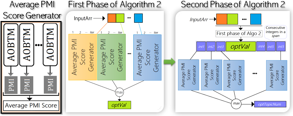
Figure 3: Two Phases of Algorithm 2, , determining the optimal topic number. Each element of the InputArr is handled by one CPU-core. Circle-max represent the reduction operator.

IV-B Algorithm Determining Number of Versions to Consider

Earlier, we have discussed how previous versions or time slices incur different contributions to the topic distributions of the latest time-slice. In AOBTM, we form the prior topic distributions for $t$-th time-slice by taking weighted contributions of the previous $win$ number of time slices into account. Users can define the parameter $win\in[1,v-1]$ in Algorithm 1, where $v$ denotes the available time slices. To make an educated decision about the parameter $win$, we can analyze the change in PMI Scores for different values of $win$. We build ($v-1$) number of AOBTM models for the latest time-slice with different values of $win$ and calculate the PMI-Scores. In the parallel block, we use OpenMp reduction clause to find the maximized PMI-score. If OpenMp is not enabled in a machine, we store the scores in an array, where the score’s index corresponds to the number of considered versions. Then, with one scan of the array, we determine the cutoff point where the PMI-score dropped and did not rise again.

We propose Algorithm 3 to determine the appropriate number of previous versions to consider automatically.

Input : $dataset,v,iter$

Output : $optVerNum$

1 Set $maxPMI\leftarrow 0.0$, $optVerNum\leftarrow 1;$

2 #pragma omp parallel for reduction(max:maxPMI)

3 for $i\leftarrow 1$ to $v-1$ do

4      Set $threadId\leftarrow omp\_get\_thread\_num();$

5       Set $win\leftarrow threadId+1;$

6       /* Each thread runs AOBTM $iter$ time by taking $win$ number of previous versions into account, calculate the PMI-Scores and saves them in PMI_final; (repeating lines 5 to 18 of Algo. 2);*/

7       if (PMI_final $>maxPMI$) then

8             optVerNum $\leftarrow w$; maxPMI $\leftarrow$ PMI_final;

9            

10      

11 end for

Algorithm 3 Optimal Number of Versions

V Experiments and Results

In this section, we evaluate the performance of AOBTM in identifying consistent and distinctive latent topics from corpora comprising of short text documents. We explain the datasets and compare the results of different topic modeling algorithms. Our focus is to answer the following research questions:

• RQ1: Can AOBTM achieve better performance compared to other topic modeling methods?

• RQ2: How do different parameter settings, document-lengths, and pre-processing approaches impact the performance of AOBTM?

• RQ3: Using the parameters set by our parallel algorithms, how discriminative and coherent are the topics discovered by different topic modeling methods?

V-A Setups

V-A1 Datasets

To show the effectiveness of our approach, in addition to using app reviews, we use a large dataset of Twitter microblogs. Tweets are considered as short text and evaluation on this dataset can show the applicability of AOBTM on short text analysis. The details of the datasets are as follows:

App Reviews from Apple Store and Google Play. We use the dataset provided by Gao et al. [10], which is previously studied to evaluate AOLDA for extracting topics from app reviews. The dataset includes reviews that are related to a number of versions of the collected apps. The subject apps are distributed in different categories and platforms; this choice ensures the generalization of our approach. We enriched the provided datasets by adding the user-reviews collected from the latest versions of the subject apps. However, one of the apps in this dataset, ”Clean Master,” was discontinued, and we could not acquire app-changelogs. Another app in the provided dataset, namely ”eBay,” had pulled enormous app-reviews from the app-stores. As the changelogs are critical to our evaluation metrics, we have decided to discard these two apps from the evaluation. We double-checked the provided app-reviews and changelogs in the dataset from the play stores and discarded the ones that could not be found. Table II summarizes the specifications of the app reviews datasets.

Tweets2020 is a collection of approximately 200,000 tweets scraped from Twitter between January 1st and May 20th, 2020, where each month is considered as a time-slice. For the collection of the tweets, we have used an open-sourced twitter-scraper . We used 300 top trending topics over the region of North America to collect the tweets with timestamp. Besides the content, each tweet includes user id, timestamp, number of retweets, and likes.

The user reviews and tweets collections contain many noisy words, such as repetitive words, casual words, misspelled words, and non-informative words (e.g., ”normally”). We have performed common text preprocessing techniques including removing meaningless words, lowercasing, lemmatization, digit and name replacement following [35]. We apply the preprocessing technique in for lemmatization and replace all digits with ”<digit>.” We also removed duplicate records and documents with a single word.

TABLE II: Subject apps from different app-stores

2.5 App Name	Category	Platform	#Reviews	#Versions
2.5 NOAA Radar	Weather	App Store	10,112	16
Youtube	Multimedia	App Store	44,531	35
Viber	Communication	Google Play	19,327	9
Swiftkey	Productivity	Google Play	23,121	17
2.5

V-A2 Baselines

We select LDA [14], BTM [16], OLDA [20], OBTM [21], and AOLDA [10] as our baseline methods to evaluate the performance of AOBTM. The details of the baseline algorithms are explained in Section II. All the experiments were carried on a Linux machine with Intel 2.21 GHz CPU and 16G memory. Following the literature [10], we have used all algorithms implemented by Gibbs sampling in C++ .

V-A3 Evaluation Metrics

Good topic models deliver coherent [28] and discriminative topics, which cover unique and comprehensive aspects of the corpus [10]. So, We utilized PMI-Score as a measure of coherence [16] and Discreteness Score (Dis_Score) to measure the discriminative property of the derived topics, which is inspired from the semantic similarity mapping in[10]. Higher values of PMI_Score and Dis_Score suggest the discovery of more coherent and discriminative topics. We also presented time-cost (seconds) per iteration (Time_Cost in Table V-B) as the third performance metric. We picked the top 10 terms from each generated topic to calculate the PMI-Scores, as explained in section IV. For calculating Dis_Score, we use Jensen Shannon (JS) Divergence $D_{JS}$ [36], to estimate the difference between two topic distributions ($\Phi$). The equations are provided below:

Eq. 7 elaborates $D_{JS}$ of Eq. 6. Eq. 8 defines the $D_{KL}$ (Kullback-Leibler Divergence) and $M$ from Eq. 7. In Eq. 6, the innter term, $\sum_{j=1,j\neq k}^{K}D_{JS}(\Phi_{k}^{t}||\Phi_{j}^{t})/K$ measures the difference of a single topic distribution’s average with the rest of the topic distributions. In Eq. 8, $P(i)$ (or $Q(i)$) is the $i$-th item in $P$ (or $Q$).

To provide a better comparison, we adopted three more performance metrics used in [10] to evaluate the performance of AOLDA. These metrics are $\mathrm{Precision_{E}}$, $\mathrm{Recall_{L}}$, and $\mathrm{F_{hybrid}}$. Further details about these metrics are discussed in [10]. For app-reviews and twitter data, we have taken app-changelogs and popular hashtags, respectively as our ground-truths. Here, $\mathrm{Precision_{E}}$ measures the accuracy in detecting emerging topics in the latest time slice, t [10]. $\mathrm{Recall_{L}}$ evaluates whether our prioritized topics (including both emerging and non-emerging) reflect the changes mentioned in the change-logs or hashtags. Higher $\mathrm{F_{hybrid}}$ suggests that the change-logs and hashtags are more explicitly covered by detected topics. The higher score in $\mathrm{F_{hybrid}}$ also signifies that the prioritized issues reflect more of the change-logs and hashtags contents [10].

V-B Result of RQ1: Comparison Results with Different Methods

Table V-B presents the evaluation results, where, $P_{E},R_{L},F_{h}$ refer to $\mathrm{Precision_{E}}$, $\mathrm{Recall_{L}}$, and $\mathrm{F_{hybrid}}$, respectively.

TABLE III: Comparison result of different methods

2.5 App-Name (#Avg. Texts)	Methods	PMI_Scores	Dis_ Scores	Time_ Cost	$P_{E}$	$R_{L}$	$F_{h}$
2.5 Tweets2020 (~39,803)	LDA	2.03 $\pm$ 0.04	0.68	43.27	NA	NA	NA
	BTM	2.04 $\pm$ 0.02	0.61	46.8	NA	NA	NA
	OLDA	1.90 $\pm$ 0.03	0.79	17.11	0.581	0.612	0.592
	OBTM	1.92 $\pm$ 0.03	0.79	21.91	0.574	0.605	0.588
	AOLDA	2.09 $\pm$ 0.03	0.89	56.7	0.603	0.677	0.657
	AOBTM	2.13 $\pm$ 0.04	0.82	63.87	0.608	0.684	0.662
2.5 NOAA Radar (~632)	LDA	1.34 $\pm$ 0.03	0.57	18.8	NA	NA	NA
	BTM	1.36 $\pm$ 0.03	0.63	22.31	NA	NA	NA
	OLDA	1.38 $\pm$ 0.03	0.68	8.25	0.461	0.519	0.47
	OBTM	1.41 $\pm$ 0.03	0.71	14.6	0.576	0.495	0.548
	AOLDA	1.45 $\pm$ 0.04	0.75	23.44	0.568	0.492	0.533
	AOBTM	1.48 $\pm$ 0.04	0.78	20.54	0.578	0.508	0.556
2.5 Youtube (~1,272)	LDA	1.56 $\pm$ 0.04	0.64	20.74	NA	NA	NA
	BTM	1.62 $\pm$ 0.04	0.73	25.36	NA	NA	NA
	OLDA	1.53 $\pm$ 0.03	0.76	11.51	0.439	0.455	0.448
	OBTM	1.55 $\pm$ 0.04	0.74	15.33	0.483	0.464	0.463
	AOLDA	1.61 $\pm$ 0.03	0.8	30.92	0.598	0.474	0.529
	AOBTM	1.66 $\pm$ 0.03	0.82	31.08	0.615	0.482	0.538
2.5 Viber (~2,147)	LDA	1.65 $\pm$ 0.03	0.68	29.06	NA	NA	NA
	BTM	1.72 $\pm$ 0.02	0.75	33.4	NA	NA	NA
	OLDA	1.58 $\pm$ 0.03	0.8	14.47	0.458	0.395	0.419
	OBTM	1.62 $\pm$ 0.02	0.82	20.32	0.417	0.308	0.365
	AOLDA	1.76 $\pm$ 0.04	0.81	34.64	0.465	0.409	0.428
	AOBTM	1.89 $\pm$ 0.03	0.85	37.55	0.572	0.411	0.508
2.5 Swiftkey (~1,360)	LDA	1.53 $\pm$ 0.02	0.67	23.18	NA	NA	NA
	BTM	1.61 $\pm$ 0.02	0.68	28.85	NA	NA	NA
	OLDA	1.42 $\pm$ 0.04	0.74	16.06	0.209	0.551	0.291
	OBTM	1.49 $\pm$ 0.04	0.73	21.55	0.313	0.52	0.392
	AOLDA	1.67 $\pm$ 0.03	0.76	29.48	0.526	0.631	0.584
	AOBTM	1.71 $\pm$ 0.02	0.83	31.26	0.542	0.658	0.591
2.5

During evaluation for RQ1, we set the parameters as $w=3$ and $K=10$ for the adaptive online algorithms for the sake of uniformity. We have initialized $\alpha=0.05$ and $\beta=0.01$ for LDA based methods as they have achieved the best performance with these values for short texts in [16]. We have set $\alpha=50/K$ and $\beta=0.01$ for BTM based algorithms [16].

From Table V-B, we observe that AOBTM delivers the highest PMI-Scores with every dataset by alleviating the data sparsity problem and considering the varying contributions of different time-slices or versions. So, the topics discovered by AOBTM are more coherent and comprehensible. For discriminative topic learning, AOBTM performs better than other methods, except for the Tweets2020 dataset. A large amount of short texts per time-slice in the Tweets2020 dataset helps AOLDA to learn better document level word correlations and infer more discriminative topics; still, AOLDA did not generate higher PMI-Score than AOBTM for Tweets2020. From the result, it is apparent that AOBTM exceeds the benchmark methods including its online version, OBTM, as well as AOLDA. Although AOBTM marginally improved the performance of AOLDA, the performance improvement of AOLDA over OLDA is approximately the same as that of AOBTM over OBTM. AOBTM also generated the highest scores for every dataset for $\mathrm{Precision_{E}}$, $\mathrm{Recall_{L}}$, and $\mathrm{F_{hybrid}}$, which indicates that our topic model can select emerging topics more precisely.

We acknowledge that AOBTM is more time-expensive than all the other baselines, but the runtime is comparable to adaptive online methods when the dataset is small. From Table V-B, we observe that the difference of runtime between AOLDA and AOBTM is trivial; AOBTM even outperforms AOLDA in runtime for NOAA Radar dataset, which has the lowest number of average short texts per version.

V-C Result of RQ2: Effect of Different Parameter Settings, Document Lengths and Preprocessing Approaches

Effect of Different Parameter Settings. In Fig. 4 and Fig. 5, we have compared our method with AOLDA, as the number of previous versions to consider is unique to adaptive online algorithms. In Fig. 4, we consider distinct uniform topic-number for each dataset and calculate PMI-Scores for the different number of previous versions. The topic numbers for the dataset is calculated by Algorithm 2. In Fig. 5, we consider fixed window-size (number of versions) to calculate the PMI-Scores for varying number of topics.

We can observe that AOBTM in general generates the highest PMI-Scores, and the trendlines of both methods are analogous. In Fig. 4, the declines in the performance of AOBTM (i.e., win=25 in YouTube dataset) can transpire for the following reasons: the emergence of an unrelated novel topic in the recently considered versions (i.e., from 20th to 25th versions in YouTube dataset), content drifting, and higher occurrence of meaningless texts in the newly included versions [21]. In Fig. 5, in all cases, the methods produced an increasing number of PMI-Scores until the tipping point generates the highest score. Once the methods reach their peak, a further increase in the number of topics generates incoherent coinciding topics inducing the reduction in PMI-Scores.

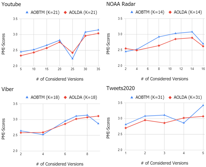
Figure 4: PMI-Scores for varying number of considered versions or time-slices.

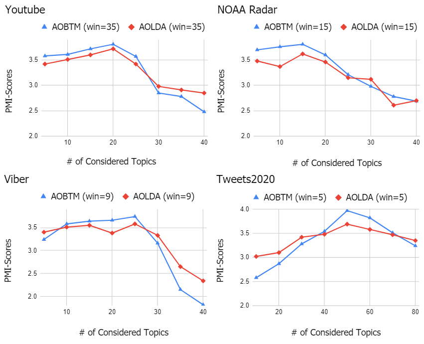
Figure 5: PMI-Scores for varying number of topics.

Effect of Document Length. In Fig. 6, we have presented AOBTM’s performance using PMI-Scores with respect to varying document lengths. We have considered average document length for each dataset to evaluate the considered methods. Tweets2020, NOAA Radar, Youtube, Viber, and Swiftkey have average document length of 68.3, 8.5, 13.6, 9.4, and 6.2, respectively. AOBTM performs better than other methods for all datasets. It is worth noting that, as expected, LDA based methods performed well with large document length and bigger corpus, mostly because of the dataset’s content richness and abundance of document level word co-occurrences.

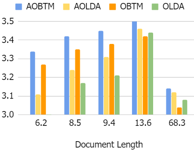
Figure 6: PMI-Scores for varying document lengths.

Effect of Preprocessing. In section III, we have mentioned a preprocessing technique with Phrase Extraction that can deliver more comprehensible top contributing terms in each discovered topic. We implement AOBTM+ with the phrase extraction preprocessing technique. In Table IV, we explicate how this technique in AOBTM+ generates better topic words than AOBTM with no phrase extraction. We selected a topic discovered from the Twitter dataset, which is related to Racism. We can see that extracting phrases during preprocessing and training them with the rest of the terms help distinguishing key terms for topic representation, which is captured only by AOBTM+.

TABLE IV: Five most contributing terms from a topic from Tweets2020

Methods	Key-Terms
AOLDA	hate, race, black, white, stop
AOBTM	black, hate, white, race, crime
AOBTM+	stop_racism, black, stop_hate, police_brutality, white_supremacy

V-D Result of RQ3: Quality of Discovered Topics Using Parameters Determined by Proposed Algorithms

In [37, 38, 39, 40], researchers have explored different ways to finetune the topic models’ parameters. Their basic approach is to train various topic models (with different parameter settings) over several iterations to select one with the best performance. All the proposed procedures are computationally expensive, especially when executed sequentially. Moreover, all the existing libraries and packages that implement the mentioned procedures use LDA based models [41]. So, we proposed two parallel algorithms as described in Section IV to determine 2 important parameters in our approach automatically: i) the number of topics to discover ($K$) and ii) the number of previous versions/time-slices to consider ($win$). In Table V, time-complexities are provided for both algorithms. It is worth noting that the proposed algorithms run sequentially if the environment is not set up to perform parallelism.

TABLE V: Time Complexities for Proposed Parallel Algorithms

	Time-Complexity
2.5 Algorithm 2	$O\big{(}[iter+span][N_{iter}K|N_{B}^{(t)}|+vKW]\big{)}$
Algorithm 3	$O\big{(}[iter][N_{iter}K|N_{B}^{(t)}|+vKW]\big{)}$

We have employed the proposed algorithms to determine the best values for the parameters $K$ and $win$ for each dataset. For Tweets2020, Youtube, Viber, NOAA, and Swiftkey, Algorithm 2 determined the corresponding numbers of topics to be derived as 31, 22, 18, 13, and 11, respectively, whereas Algorithm 3 determined the best $win$ value to be considered as 5, 34, 9, 16, and 11, respectively. After setting the best detected parameters for the online and adaptively online algorithms, we have calculated the PMI-Scores for each dataset and present the results in Fig. 7. The plot shows that AOBTM outperforms all the other online algorithms for all datasets. Compared to OBTM, AOLDA and OLDA perform better for datasets that contain longer documents. Furthermore, OBTM outperforms both of the LDA based methods when it comes to the limited datasets containing short texts.

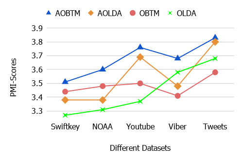
Figure 7: PMI-Scores generated by setting the parameters determined by Algorithms 2 and 3

V-E Real-World Application

Prompt detection of emerging topics from user reviews is crucial for app developers as these topics reveal users’ requirements, preferences, and complaints [10]. Developers can proactively identify user-complaints and take quick actions to improve user experience through efficient analysis of the app-reviews. Timely and precisely identifying emerging issues helps developers to fix bugs, refine existing features, and add essential functions in the subsequent update of the application. For this purpose, Gao et al. developed a framework named IDEA to detect emerging issues from the app-reviews of popular applications [10]. IDEA collects user reviews after the publication of different versions of the app and implement AOLDA to get the topic-word distributions for the app reviews collected after the publication of the latest version. We have modified the open-source framework IDEA and incorporated AOBTM instead of AOLDA to generate the topic-word distribution. The rest of the framework’s components, such as preprocessing, emerging topic identification, and topic interpretation, remain the same. The modified version is denoted as OPRA (Online App Review Analysis).

TABLE VI: Five most contributing terms from two sample topics

Topics	IDEA	OPRA
Topic 1	password	zoombomb
	meeting	password
	abuse	security
	attack	policy
	policy	disturb
Topic 2	message	group chat
	status	message
	channel	notification
	chat	transfer
	link	link

Inspired by the zoom case study as explained in Section I, we have collected around 15,000 app reviews for Zoom Cloud Meetings from Google Play. The average review length for this dataset is 7.8. These reviews were generated after the publication of the latest 5 versions of the app. For emerging topic detection, we set the parameters as $win=3$ and $K=10$ for fair evaluation. We also changed the initial values of $\alpha$ and $\beta$ to 0.1 and 0.01, respectively, as these values yielded best performance for IDEA (implementing AOLDA) in [10].

In Table VI, we have reported top 5 most contributing words from two topics generated by IDEA and OPRA: first topic is closely related to app-security, and second topic is closely related to messaging feature of the app. In Table VII, we have reported the corresponding PMI-Scores and Time-Cost for both frameworks. We can see that applying AOBTM in the framework slightly increases the time-cost, but generates more comprehensive and coherent topics.

TABLE VII: PMI-Scores & Time Cost evaluation for Zoom app-reviews

Frameworks	PMI Score	Time Cost	$\mathrm{Precision_{E}}$	$\mathrm{Recall_{L}}$	$\mathrm{F_{hybrid}}$
IDEA	2.08	12.52	0.572	0.608	0.586
OPRA	2.35	16.8	0.593	0.619	0.608

VI Related Work

For the topic modeling for short texts, PLSA, LDA, and their variants suffer from the lack of enough word co-occurrences. To boost the performance of topic models, researchers had utilized external knowledge to produce supplementary essential word co-occurrences across short texts [42, 43, 44]. The problem rests in that auxiliary information can be too scarce or too expensive (or both) for deployment.

In the short text topic modeling regime, Yin at al. introduced the DMM based topic modeling method in [45], where it is presumed that each short-text is sampled from only one latent topic. But this proved to be too simple and too strong of an assumption for any reasonable short text topic model [46]. In self-aggregation based methods, short texts are merged into long pseudo-documents before topic inference to help develop rich word co-occurrence information. Researchers have used this type of method in [47, 48], where they have presumed that each short text is sampled from a long concatenated pseudo-document (unobserved in current text collection). This presumption enables inferring latent topics from long pseudo-documents. But the concatenation yielded suboptimal results in [49, 50] as merging short texts into long pseudo-documents using word embeddings cannot alleviate the loss of auxiliary information or metadata. Global word co-occurrences based methods (i.e., [16, 51]) try to use the rich global word co-occurrence patterns for inferring latent topics, where the adequacy of these co-occurrences alleviates the sparsity problem of short texts. [16] posits that the two words in a biterm share the same topic drawn from a mixture of topics over the whole corpus. This topic modeling algorithm is comparatively more robust and suitable for all the mentioned characteristics of short texts [52].

To solve the problems with streaming short texts and unordered topic generation, researchers proposed online models such as OLDA [20] and Online BTM [16]. In essence, online algorithms fit conventional topic models (i.e., BTM, LDA, respectively) over the data in a time-slice $t$ and use the inferred statistical data to adjust Dirichlet hyperparameters for the next time slice.

Gao et al. [10] introduced the Adaptively Online LDA (AOLDA) by factoring in all the previous time-slices’ contribution, instead of just the preceding one. Here, they have shown that the comparison among the topic distributions for more than two consecutive time-slices/versions can lead to more coherent and distinguishable topic learning. But this specific method uses LDA as their underlying topic model, which suffers from several discussed issues when it comes to short texts [16].

VII Threats to validity

Human Evaluation. In our experiments, we have only used deterministic scores to evaluate our results against the benchmarks. The authors of this paper have manually reviewed the outcomes of the considered topic models. We have consulted with fellow researchers about the model outcome and have considered the opinions of industry developers which confirmed that AOBTM generates more coherent key-words for extracted topics. But we did not perform any formal human evaluation to assess how well our model performs in practice compared to others.

Datasets. Our proposed topic models with text corpus distributed over different versions or time-slices. Evaluating our models using only version-tagged app-reviews from mobile applications that have multiple published versions in the app-store would not give us a precise idea about how this algorithm works with time slices. We have handled the problem by We have evaluated our approach using a few mobile applications, which might affect the generality of our model. To migrate the problem, we have incorporated a new dataset with around 200,000 timeline-tagged tweets scraped by considering 300 top trending topics from Canada and the USA. Furthermore, we carefully selected apps so that we could demonstrate out topic model’s performance for apps that have small or large number of reviews per version (~623-2,147)

Ground Truth. To measure the extensibility of our topic model, we wanted to know how it scales to other online algorithms for prioritizing topics and detecting emerging ones. For selecting ground-truth, we have used key-terms from app-changelogs for app-reviews, as Gao et al. did in [10]. In order to calculate precision, recall, and F-score, app-changelogs are used as ground truth, similar to [10]. However, we did not have any changelogs or tweet-summary to take as ground-truth for Tweets2020. We have manually selected top-trending hashtags over different time-slices to mine the key-terms. Other approaches for evaluation should be studied.

Memory and Time Cost. We acknowledge that our model cannot compare to the benchmarks when it comes to memory and time-cost. Still, we are currently endeavoring to incorporate word-cooccurrence pattern algorithm to make our topic model faster while using significantly less resources.

VIII Conclusion and Future Work

In this paper, we proposed a novel adaptive topic modeling algorithm, AOBTM, which is able to discover coherent and discriminative topics from short texts. AOBTM addresses the problems with conventional topic models by adopting a version sensitive strategy. Along with AOBTM, we use a preprocessing technique that enables capturing distinguishable terms in an extracted topic. Moreover, we implemented two parallel algorithms to determine the value of the two most important parameters of our model automatically. The results of several experiments on app reviews and Twitter datasets confirm the performance of AOBTM compared to the state of the art algorithms.

We plan to improve the underlying BTM method using short text expansion and concept drifting detection and integrate it with a topic visualization tool specifically designed for app reviews. For the parallel algorithms, we plan to use GPU-cores and shared memory cache to make the program run faster. We are currently endeavoring to incorporate word-cooccurrence pattern algorithm to make our topic model faster while using significantly less resources.

References

- [1] C. Gao, J. Zeng, D. Lo, C.-Y. Lin, M. R. Lyu, and I. King, “Infar: Insight extraction from app reviews,” in Proceedings of the 2018 26th ACM Joint Meeting on European Software Engineering Conference and Symposium on the Foundations of Software Engineering, 2018, pp. 904–907.
- [2] X. Gu and S. Kim, ““what parts of your apps are loved by users?”,” in Proceedings of the 30th IEEE/ACM International Conference on Automated Software Engineering, ser. ASE ’15. IEEE Press, 2015, p. 760–770. [Online]. Available: https://doi.org/10.1109/ASE.2015.57
- [3] N. Chen, J. Lin, S. C. Hoi, X. Xiao, and B. Zhang, “Ar-miner: mining informative reviews for developers from mobile app marketplace,” in Proceedings of the 36th international conference on software engineering, 2014, pp. 767–778.
- [4] W. Martin, F. Sarro, Y. Jia, Y. Zhang, and M. Harman, “A survey of app store analysis for software engineering,” IEEE transactions on software engineering, vol. 43, no. 9, pp. 817–847, 2016.
- [5] F. Palomba, M. Linares-Vasquez, G. Bavota, R. Oliveto, M. Di Penta, D. Poshyvanyk, and A. De Lucia, “User reviews matter! tracking crowdsourced reviews to support evolution of successful apps,” in 2015 IEEE international conference on software maintenance and evolution (ICSME). IEEE, 2015, pp. 291–300.
- [6] D. Pagano and W. Maalej, “User feedback in the appstore: An empirical study,” in 2013 21st IEEE international requirements engineering conference (RE). IEEE, 2013, pp. 125–134.
- [7] W. Maalej and H. Nabil, “Bug report, feature request, or simply praise? on automatically classifying app reviews,” in 2015 IEEE 23rd international requirements engineering conference (RE). IEEE, 2015, pp. 116–125.
- [8] L. Carreño and K. Winbladh, “Analysis of user comments: An approach for software requirements evolution,” in International Conference on Software Engineering, 05 2013, pp. 582–591.
- [9] C. Gao, W. Zheng, Y. Deng, D. Lo, J. Zeng, M. R. Lyu, and I. King, “Emerging app issue identification from user feedback: Experience on wechat,” in Proceedings of the 41st International Conference on Software Engineering: Software Engineering in Practice, ser. ICSE-SEIP ’19. IEEE Press, 2019, p. 279–288. [Online]. Available: https://doi.org/10.1109/ICSE-SEIP.2019.00040
- [10] C. Gao, J. Zeng, M. R. Lyu, and I. King, “Online app review analysis for identifying emerging issues,” in Proceedings of the 40th International Conference on Software Engineering, ser. ICSE ’18. New York, NY, USA: Association for Computing Machinery, 2018, p. 48–58. [Online]. Available: https://doi.org/10.1145/3180155.3180218
- [11] S. Hassan, C.-P. Bezemer, and A. E. Hassan, “Studying bad updates of top free-to-download apps in the google play store,” IEEE Transactions on Software Engineering, 2018.
- [12] D. Hakim and N. Singer. (2020, March) New york attorney general looks into zoom’s privacy practices. [Online]. Available: https://www.nytimes.com/2020/03/30/technology/new-york-attorney-general-zoom-privacy.html
- [13] E. Noei, F. Zhang, and Y. Zou, “Too many user-reviews, what should app developers look at first?” IEEE Transactions on Software Engineering, 2019.
- [14] D. M. Blei, A. Y. Ng, and M. I. Jordan, “Latent dirichlet allocation,” J. Mach. Learn. Res., vol. 3, no. null, p. 993–1022, Mar. 2003.
- [15] T. Hofmann, “Probabilistic latent semantic indexing,” SIGIR Forum, vol. 51, no. 2, p. 211–218, Aug. 2017. [Online]. Available: https://doi.org/10.1145/3130348.3130370
- [16] X. Cheng, X. Yan, Y. Lan, and J. Guo, “Btm: Topic modeling over short texts,” IEEE Transactions on Knowledge and Data Engineering, vol. 26, no. 12, pp. 2928–2941, 2014.
- [17] J. Boyd-Graber and D. Blei, “Syntactic topic models,” in Proceedings of the 21st International Conference on Neural Information Processing Systems, ser. NIPS’08. Red Hook, NY, USA: Curran Associates Inc., 2008, p. 185–192.
- [18] X. Wang and A. McCallum, “Topics over time: A non-markov continuous-time model of topical trends,” in Proceedings of the 12th ACM SIGKDD International Conference on Knowledge Discovery and Data Mining, ser. KDD ’06. New York, NY, USA: Association for Computing Machinery, 2006, p. 424–433. [Online]. Available: https://doi.org/10.1145/1150402.1150450
- [19] L. Hong and B. D. Davison, “Empirical study of topic modeling in twitter,” in Proceedings of the First Workshop on Social Media Analytics, ser. SOMA ’10. New York, NY, USA: Association for Computing Machinery, 2010, p. 80–88. [Online]. Available: https://doi.org/10.1145/1964858.1964870
- [20] M. D. Hoffman, D. M. Blei, and F. Bach, “Online learning for latent dirichlet allocation,” in Proceedings of the 23rd International Conference on Neural Information Processing Systems - Volume 1, ser. NIPS’10. Red Hook, NY, USA: Curran Associates Inc., 2010, p. 856–864.
- [21] X. Hu, H. Wang, and P. Li, “Online biterm topic model based short text stream classification using short text expansion and concept drifting detection,” Pattern Recognition Letters, vol. 116, 10 2018.
- [22] Q. Jipeng, Q. Zhenyu, L. Yun, Y. Yunhao, and W. Xindong, “Short text topic modeling techniques, applications, and performance: A survey,” 2019.
- [23] D. M. Blei, “Probabilistic topic models,” Commun. ACM, vol. 55, no. 4, p. 77–84, Apr. 2012. [Online]. Available: https://doi.org/10.1145/2133806.2133826
- [24] P. Xie and E. P. Xing, “Integrating document clustering and topic modeling,” in Proceedings of the Twenty-Ninth Conference on Uncertainty in Artificial Intelligence, ser. UAI’13. Arlington, Virginia, USA: AUAI Press, 2013, p. 694–703.
- [25] P. Xie, D. Yang, and E. Xing, “Incorporating word correlation knowledge into topic modeling,” in Proceedings of the 2015 Conference of the North American Chapter of the Association for Computational Linguistics: Human Language Technologies. Denver, Colorado: Association for Computational Linguistics, May–Jun. 2015, pp. 725–734. [Online]. Available: https://www.aclweb.org/anthology/N15-1074
- [26] T. Lin, W. Tian, Q. Mei, and H. Cheng, “The dual-sparse topic model: Mining focused topics and focused terms in short text,” in Proceedings of the 23rd International Conference on World Wide Web, ser. WWW ’14. New York, NY, USA: Association for Computing Machinery, 2014, p. 539–550. [Online]. Available: https://doi.org/10.1145/2566486.2567980
- [27] J. H. Lau, D. Newman, S. Karimi, and T. Baldwin, “Best topic word selection for topic labelling,” in Proceedings of the 23rd International Conference on Computational Linguistics: Posters, ser. COLING ’10. USA: Association for Computational Linguistics, 2010, p. 605–613.
- [28] Q. Mei, X. Shen, and C. Zhai, “Automatic labeling of multinomial topic models,” in Proceedings of the 13th ACM SIGKDD International Conference on Knowledge Discovery and Data Mining, ser. KDD ’07. New York, NY, USA: Association for Computing Machinery, 2007, p. 490–499. [Online]. Available: https://doi.org/10.1145/1281192.1281246
- [29] D. Newman, J. H. Lau, K. Grieser, and T. Baldwin, “Automatic evaluation of topic coherence,” in Human Language Technologies: The 2010 Annual Conference of the North American Chapter of the Association for Computational Linguistics, ser. HLT ’10. USA: Association for Computational Linguistics, 2010, p. 100–108.
- [30] G. Heinrich, “Parameter estimation for text analysis,” Technical report, Tech. Rep., 2005.
- [31] A. Gruber, Y. Weiss, and M. Rosen-Zvi, “Hidden topic markov models,” in Artificial intelligence and statistics, 2007, pp. 163–170.
- [32] T. L. Griffiths, M. Steyvers, D. M. Blei, and J. B. Tenenbaum, “Integrating topics and syntax,” in Advances in neural information processing systems, 2005, pp. 537–544.
- [33] J. Chang, J. Boyd-Graber, S. Gerrish, C. Wang, and D. M. Blei, “Reading tea leaves: How humans interpret topic models,” in Proceedings of the 22nd International Conference on Neural Information Processing Systems, ser. NIPS’09. Red Hook, NY, USA: Curran Associates Inc., 2009, p. 288–296.
- [34] D. Mimno, H. M. Wallach, E. Talley, M. Leenders, and A. McCallum, “Optimizing semantic coherence in topic models,” in Proceedings of the Conference on Empirical Methods in Natural Language Processing, ser. EMNLP ’11. USA: Association for Computational Linguistics, 2011, p. 262–272.
- [35] Y. Man, C. Gao, M. R. Lyu, and J. Jiang, “Experience report: Understanding cross-platform app issues from user reviews,” in 2016 IEEE 27th International Symposium on Software Reliability Engineering (ISSRE), 2016, pp. 138–149.
- [36] “Jensen–shannon divergence,” April 2020. [Online]. Available: https://en.wikipedia.org/wiki/Jensen-Shannon_divergence
- [37] R. Arun, V. Suresh, C. E. Veni Madhavan, and M. N. Narasimha Murthy, “On finding the natural number of topics with latent dirichlet allocation: Some observations,” in Proceedings of the 14th Pacific-Asia Conference on Advances in Knowledge Discovery and Data Mining - Volume Part I, ser. PAKDD’10. Berlin, Heidelberg: Springer-Verlag, 2010, p. 391–402. [Online]. Available: https://doi.org/10.1007/978-3-642-13657-3_43
- [38] J. Cao, T. Xia, J. Li, Y. Zhang, and S. Tang, “A density-based method for adaptive lda model selection,” Neurocomput., vol. 72, no. 7–9, p. 1775–1781, Mar. 2009. [Online]. Available: https://doi.org/10.1016/j.neucom.2008.06.011
- [39] R. Deveaud, E. SanJuan, and P. Bellot, “Accurate and effective latent concept modeling for ad hoc information retrieval,” Document numérique, vol. 17, no. 1, pp. 61–84, 2014.
- [40] T. L. Griffiths and M. Steyvers, “Finding scientific topics,” Proceedings of the National academy of Sciences, vol. 101, no. suppl 1, pp. 5228–5235, 2004.
- [41] M. Ponweiser, “Latent dirichlet allocation in r,” WU Vienna University Journal, 2012.
- [42] O. Jin, N. N. Liu, K. Zhao, Y. Yu, and Q. Yang, “Transferring topical knowledge from auxiliary long texts for short text clustering,” in Proceedings of the 20th ACM International Conference on Information and Knowledge Management, ser. CIKM ’11. New York, NY, USA: Association for Computing Machinery, 2011, p. 775–784. [Online]. Available: https://doi.org/10.1145/2063576.2063689
- [43] X.-H. Phan, L.-M. Nguyen, and S. Horiguchi, “Learning to classify short and sparse text & web with hidden topics from large-scale data collections,” in Proceedings of the 17th International Conference on World Wide Web, ser. WWW ’08. New York, NY, USA: Association for Computing Machinery, 2008, p. 91–100. [Online]. Available: https://doi.org/10.1145/1367497.1367510
- [44] R. Mehrotra, S. Sanner, W. Buntine, and L. Xie, “Improving lda topic models for microblogs via tweet pooling and automatic labeling,” in Proceedings of the 36th International ACM SIGIR Conference on Research and Development in Information Retrieval, ser. SIGIR ’13. New York, NY, USA: Association for Computing Machinery, 2013, p. 889–892. [Online]. Available: https://doi.org/10.1145/2484028.2484166
- [45] J. Yin and J. Wang, “A dirichlet multinomial mixture model-based approach for short text clustering,” in Proceedings of the 20th ACM SIGKDD International Conference on Knowledge Discovery and Data Mining, ser. KDD ’14. New York, NY, USA: Association for Computing Machinery, 2014, p. 233–242. [Online]. Available: https://doi.org/10.1145/2623330.2623715
- [46] W. X. Zhao, J. Jiang, J. Weng, J. He, E.-P. Lim, H. Yan, and X. Li, “Comparing twitter and traditional media using topic models,” in Proceedings of the 33rd European Conference on Advances in Information Retrieval, ser. ECIR’11. Berlin, Heidelberg: Springer-Verlag, 2011, p. 338–349.
- [47] X. Quan, C. Kit, Y. Ge, and S. J. Pan, “Short and sparse text topic modeling via self-aggregation,” in Proceedings of the 24th International Conference on Artificial Intelligence, ser. IJCAI’15. AAAI Press, 2015, p. 2270–2276.
- [48] Y. Zuo, J. Wu, H. Zhang, H. Lin, F. Wang, K. Xu, and H. Xiong, “Topic modeling of short texts: A pseudo-document view,” in Proceedings of the 22nd ACM SIGKDD International Conference on Knowledge Discovery and Data Mining, ser. KDD ’16. New York, NY, USA: Association for Computing Machinery, 2016, p. 2105–2114. [Online]. Available: https://doi.org/10.1145/2939672.2939880
- [49] C. Li, H. Wang, Z. Zhang, A. Sun, and Z. Ma, “Topic modeling for short texts with auxiliary word embeddings,” in Proceedings of the 39th International ACM SIGIR Conference on Research and Development in Information Retrieval, ser. SIGIR ’16. New York, NY, USA: Association for Computing Machinery, 2016, p. 165–174. [Online]. Available: https://doi.org/10.1145/2911451.2911499
- [50] P. Bicalho, M. Pita, G. Pedrosa, A. Lacerda, and G. L. Pappa, “A general framework to expand short text for topic modeling,” Inf. Sci., vol. 393, no. C, p. 66–81, jul 2017.
- [51] Y. Zuo, J. Zhao, and K. Xu, “Word network topic model: A simple but general solution for short and imbalanced texts,” Knowl. Inf. Syst., vol. 48, no. 2, p. 379–398, Aug. 2016. [Online]. Available: https://doi.org/10.1007/s10115-015-0882-z
- [52] C. Li, Y. Duan, H. Wang, Z. Zhang, A. Sun, and Z. Ma, “Enhancing topic modeling for short texts with auxiliary word embeddings,” ACM Trans. Inf. Syst., vol. 36, no. 2, Aug. 2017. [Online]. Available: https://doi.org/10.1145/3091108