Time imaging reconstruction for the PANDA Barrel DIRC

Abstract

The innovative Barrel DIRC (Detection of Internally Reflected Cherenkov light) counter will provide hadronic particle identification (PID) in the central region of the PANDA experiment at the new Facility for Antiproton and Ion Research (FAIR), Darmstadt, Germany. This detector is designed to separate charged pions and kaons with at least 3 standard deviations for momenta up to 3.5 GeV/c, covering the polar angle range of $22^{\circ}-140^{\circ}$. An array of microchannel plate photomultiplier tubes is used to detect the location and arrival time of the Cherenkov photons with a position resolution of 2 mm and time precision of about 100 ps. The time imaging reconstruction has been developed to make optimum use of the observables and to determine the performance of the detector. This reconstruction algorithm performs particle identification by directly calculating the maximum likelihoods using probability density functions based on detected photon propagation time in each pixel, determined directly from the data, or analytically, or from detailed simulations.

1 Introduction

The PANDA Barrel DIRC [1, 2] is a key component of the particle identification (PID) system for the PANDA detector [3], which will be installed at the Facility for Antiproton and Ion Research (FAIR) in Germany. The PID goal for the Barrel DIRC is to reach 3 standard deviations (s.d.) $\pi/K$ separation for momenta up to 3.5 GeV/c, covering the polar angle range of $22^{\circ}-140^{\circ}$.

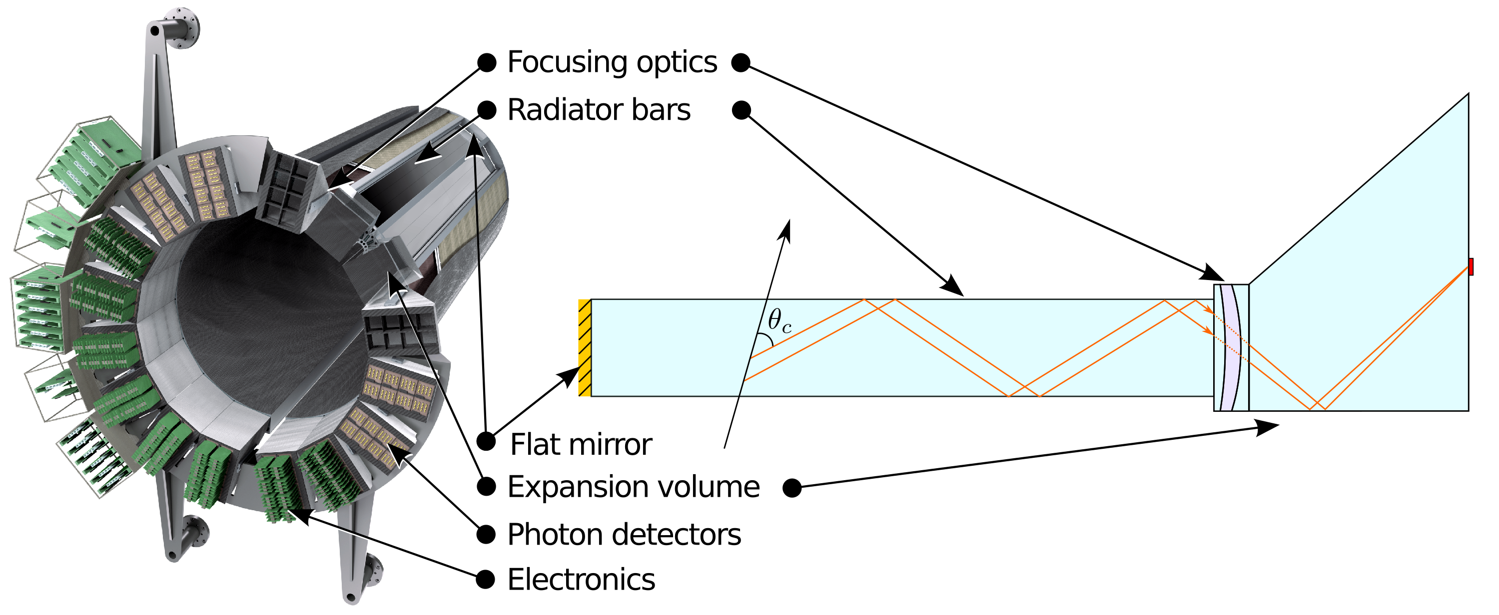
Figure 1: Rendered CAD drawing of the PANDA Barrel DIRC (left) and the simplified cross section of one Barrel DIRC sector (right, not to scale).

The Barrel DIRC is constructed in the shape of a barrel using 16 optically isolated sectors, each comprising a radiator box and a compact, prism-shaped expansion volume (EV) (see figure 1). The radiator box contains three synthetic fused silica bars of 17 $\times$ 53 $\times$ 2400 mm³ size, positioned side-by-side with a small air gap between them. A flat mirror at the forward end of each bar is used to reflect Cherenkov photons to the read-out end, where a 3-layer spherical lens images them on an array of 8 Microchannel Plate Photomultiplier Tubes (MCP-PMTs). The MCP-PMT has 64 pixels of 6.5 $\times$ 6.5 mm² size and, in combination with the FPGA-based readout electronics, will be able to detect single photons with a precision of about $100$ ps.

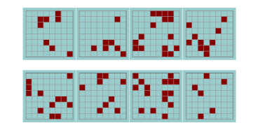
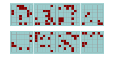
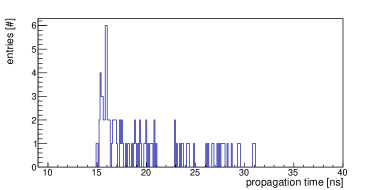
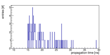
Figure 2: Hit patterns (top) and time spectra (bottom) for a single pion (left) and kaon (right) at $22^{\circ}$ polar angle and 3.5 GeV/c momentum.

Depending on the polar angle and momentum of the charged particle, the system detects 20-100 photons. Figure 2 shows a typical hit pattern and time spectra for a single pion (left) and kaon (right) at $22^{\circ}$ polar angle and 3.5 GeV/c momentum. Using this information in combination with knowledge of the charged particle momentum and direction, the reconstruction algorithms perform particle identification (PID). Two algorithms have been developed to make optimum use of the observables and to determine the performance of the detector. The "geometrical reconstruction" [4], initially developed for the BaBar DIRC [5], performs PID by reconstructing the value of the Cherenkov angle and using it in a track-by-track maximum likelihood fit, relying mostly on the position of the detected photons in the reconstruction, using the time information primarily to suppress backgrounds. The "time imaging" utilizes both, position and time information, and directly performs the maximum likelihood fit.

2 Time Imaging Reconstruction

The time imaging method is based on the approach used by the Belle II time-of-propagation (TOP) counter [7]. The basic concept is that the measured arrival time of Cherenkov photons in each single event is compared to the expected photon arrival time for every pixel and for every particle hypothesis, yielding the PID likelihoods. Figure 3 shows an example of the accumulated hit pattern and the propagation time spectra for 30k simulated pions and kaons for one specific pixel. The arrival time of the Cherenkov photons produced by $e$, $\mu$, $\pi$, K, and p is normalized for every pixel to produce probability density functions (PDFs). The total PID likelihood is then calculated as:

$$\log\mathcal{L}_{h}=\displaystyle\sum^{N}_{i=1}\log\big{(}S_{h}(p_{i},t_{i})+B(p_{i})\big{)}+\log P_{h}(N),$$ (2.1)

where $N$ is the number of detected photons in a given event, $S_{h}(p_{i},t_{i})$ is the PDF for a pixel $p_{i}$ and particle type $h$, and $B(p_{i})$ is the expected background contribution, which includes MCP-PMT dark noise and accelerator background.

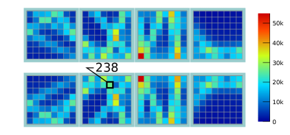
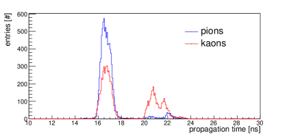
Figure 3: Accumulated hit pattern (left) and the propagation time spectra for one example pixel, number 238 (right), for 30k pions and kaons simulated at $22^{\circ}$ polar angle and 3.5 GeV/c momentum.

The second term in Eq. 2.1 is the Poisson distribution, which accounts for a difference in photon yields of different particle types. This contribution can be quite significant at low momenta but is negligible at higher momenta, where the photon yield is almost independent of the particle type.

3 Probability Density Functions

The PDFs are created from the photon arrival time, which can be obtained in several ways. The best PID performance is expected from the PDFs created using propagation times from the experimental data. In this case, the propagation time is a direct measurement which already includes all detector imperfections and, therefore, provides the most realistic PDFs. In this method a large amount of data for the whole angular and momentum acceptance is required. If the amount of experimental data is not sufficient, a full detector simulation can be used to pre-generate a large number of tracks. Both methods require a large amount of memory to store all possible PDFs and, therefore, are not practical for application in PANDA. The full simulation can also be performed during reconstruction for each event with a given track direction but excessive simulation time makes it, again, impractical to use.

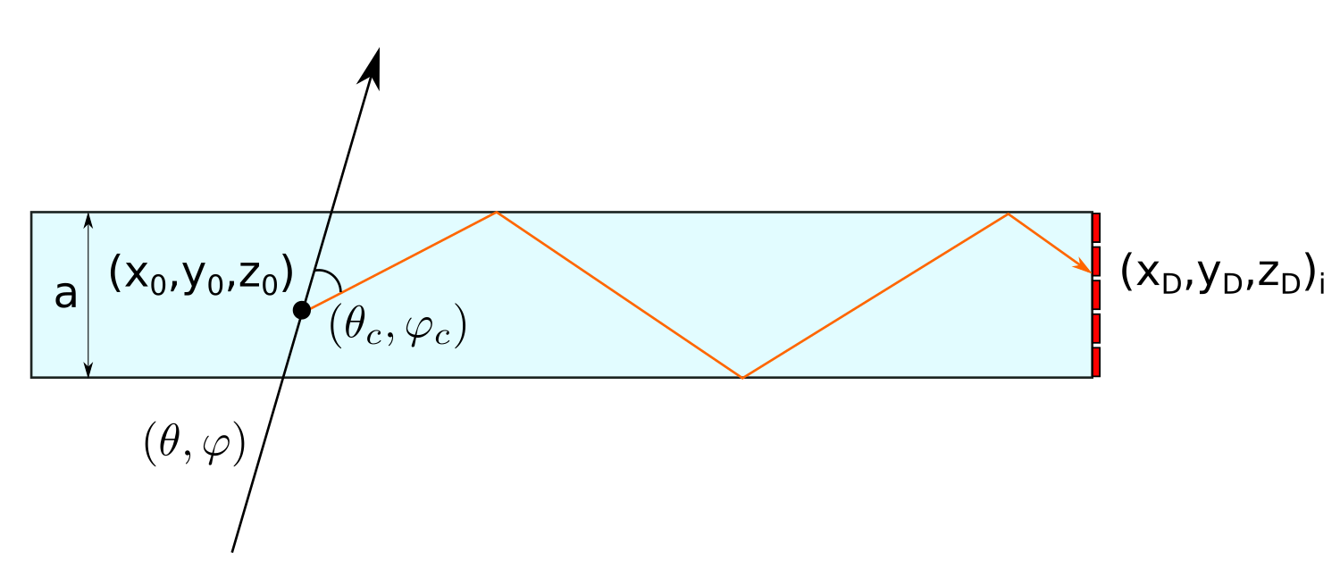
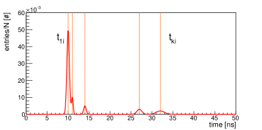
Figure 4: Simplified detector configuration without expansion volume and focusing system (left). Example of a PDF as a superposition of Gaussians with mean values $t_{ki}$ (right).

Finally, the PDFs can be calculated analytically, as shown by the Belle II TOP group [7]. In this case, the PDF $S_{h}$ is represented as a sum of $m_{i}$ weighted Gaussians:

$$S_{h}(p_{i},t_{i})=\sum^{m_{i}}_{k=0}n_{ki}g(t_{ki},\sigma_{ki}),$$ (3.1)

where $n_{ki}$ is the number of photons in the $k$-th peak of the pixel $i$, $t_{ki}$ and $\sigma_{ki}$ are position and width of the peak, respectively.

Considering a simplified configuration without expansion volume and without focusing system (see figure 4, left), the positions of the Gaussian peaks can be expressed through the direction of the charged track ($\theta,\varphi$), the Cherenkov angle $\theta_{c}$ of the assumed particle hypothesis, and the positions of the emission ($x_{0},y_{0},z_{0}$) and detection ($x_{d},y_{d},z_{d}$) of the Cherenkov photons:

$$\begin{split}&t_{ki}=\frac{z_{d}-z_{0}}{\big{(}\cos\theta\cos\theta_{c}-\sin\theta\sin\theta_{c}\cos\phi^{ki}_{c}\big{)}}\frac{n_{g}}{c_{0}},\end{split}$$ (3.2)

where $n_{g}$ is the group refractive index of the radiator, $c_{0}$ is the speed of light in vacuum, and $\phi^{ki}_{c}$ is the azimuthal angle of the Cherenkov photon in the charged particle’s coordinate system, which is defined as:

$$\begin{split}&\cos\phi^{ki}_{c}=\frac{a_{ki}b_{ki}\pm d\sqrt{d^{2}+b^{2}_{ki}-a^{2}_{ki}}}{b^{2}_{ki}+d^{2}},\end{split}$$ (3.3)

where

$$\begin{split}&a_{ki}=\frac{x^{ki}_{d}-x_{0}}{z_{d}-z_{0}}\cos\theta\cos\theta_{c}-\cos\varphi\sin\theta\cos\theta_{c},\\ &b_{ki}=\frac{x^{ki}_{d}-x_{0}}{z_{d}-z_{0}}\sin\theta\sin\theta_{c}+\cos\varphi\cos\theta\sin\theta_{c},\\ &d=\sin\varphi\sin\theta_{c}.\end{split}$$ (3.4)

Here the value of $x^{ki}_{d}$ represents the exit position of the Cherenkov photon in the unfolded radiator plane at $z_{d}$:

$$x^{ki}_{d}=\begin{cases}ka+x^{i}_{d},&k=0,\pm 2,\pm 4,...\\ ka-x^{i}_{d},&k=\pm 1,\pm 3,...,\end{cases}$$ (3.5)

where $k$ is the number of reflections inside the radiator and is a running parameter.

The width $\sigma_{ki}$ includes contributions from the photon emission spread $\Delta\lambda$, multiple scattering $\Delta\theta$, chromatic error $\Delta\sigma_{e}$, pixel size $\Delta x^{i}_{d}$ and the propagation time measurement error $\sigma_{\mathrm{m}}$:

$$\sigma_{ki}=\sqrt{\left(\frac{\partial t_{ki}}{\partial\lambda}\right)^{2}\Delta\lambda^{2}+\left(\frac{\partial t_{ki}}{\partial\theta}\right)^{2}\Delta\theta^{2}+\left(\frac{\partial t_{ki}}{\partial\sigma_{e}}\right)^{2}\Delta\sigma^{2}_{e}+\left(\frac{\partial t_{ki}}{\partial x^{i}_{d}}\right)^{2}\Delta x^{i2}_{d}+\sigma^{2}_{\mathrm{m}}}.$$ (3.6)

Finally, the number of photons in each peak is defined as:

$$n_{ki}=N_{0}l\sin^{2}\theta_{c}\frac{\Delta\phi^{ki}_{c}}{2\pi},$$ (3.7)

where $N_{0}$ is the Cherenkov photon production constant, $l$ is the length of the charged particle trajectory in the radiator, and $\Delta\phi^{ki}_{c}$ is the range of the Cherenkov azhimuthal angle coverage of the $i$-th pixel.

By adding the expansion volume and focusing system, the positions of the photons exiting the radiator $(x_{d},y_{d},z_{d})_{i}$ become ambiguous. An additional running parameter can be used to mitigate this but it will significantly slow down the reconstruction speed. Instead, a look up table (LUT) is used to determine the exit direction of the Cherenkov photon from the radiator. The LUT is constructed using Geant4 [8] simulations and comprises all possible directions from the end of radiator which can lead to a hit in a given pixel. The Gaussian mean $t_{ki}$ then can be determined as (see also figure 5, left):

$$t_{ki}=\frac{z}{\cos\beta_{ki}}\frac{n_{g}}{c_{0}}+t^{L}_{ki},$$ (3.8)

where $z$ is the distance from the photon emission point to the readout end of the radiator and $t^{L}_{ki}$ is the propagation time of the photon inside the expansion volume, which is also stored in the LUT.

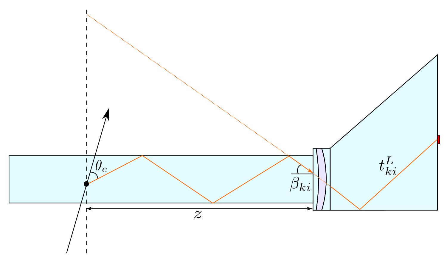
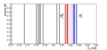
Figure 5: Detector configuration with an expansion volume and focusing (left). Example of the LUT solutions with a selection based on the reconstructed Cherenkov angle (right). Vertical black lines show the values of the reconstructed Cherenkov angle for one detected photon. Shaded red and blue areas show the selection around the expected Cherenkov angle for kaons and pions, respectively.

The tagging of the determined Gaussian peaks $g(t_{ki},\sigma_{ki})$ with a particle hypothesis is done by reconstructing the Cherenkov angle $\theta^{\mathrm{LUT}}_{c}$ using the geometrical method [4] and comparing it to the expected value of the given particle hypothesis $\theta^{h}_{c}$ (see also figure 5, right):

$$\left|\theta^{h}_{c}-\theta^{\mathrm{LUT}}_{c}\right|<w\sigma_{\mathrm{SPR}},$$ (3.9)

where $\sigma_{\mathrm{SPR}}$ is the single photon resolution of the DIRC counter, and $w$ is the selection constant, which varies in a range of 0.3-1 depending on the polar angle of the charged particle.

The construction of the PDF $S_{h}$ for a given particle hypothesis is done using Eq. 3.1 with $t_{ki}$ from Eq. 3.8 which survives the Cherenkov angle selection Eq. 3.9.

4 Performance

The performance of the algorithm was evaluated with Geant4 simulation of the prototype configuration which was tested with a $\pi/p$ beam at CERN PS in 2018 [9] (see figure 6). The Barrel DIRC prototype contained all relevant parts of one PANDA Barrel DIRC sector. A narrow fused silica bar (17.1 $\times$ 35.9 $\times$ 1200.0 mm³) was used as radiator. It coupled on one end to a flat mirror, on the other end to a 3-layer spherical focusing lens with a fused silica prism as EV. An array of 2$\times$4 MCP-PMTs attached to the back side of the EV was used to detect Cherenkov photons.

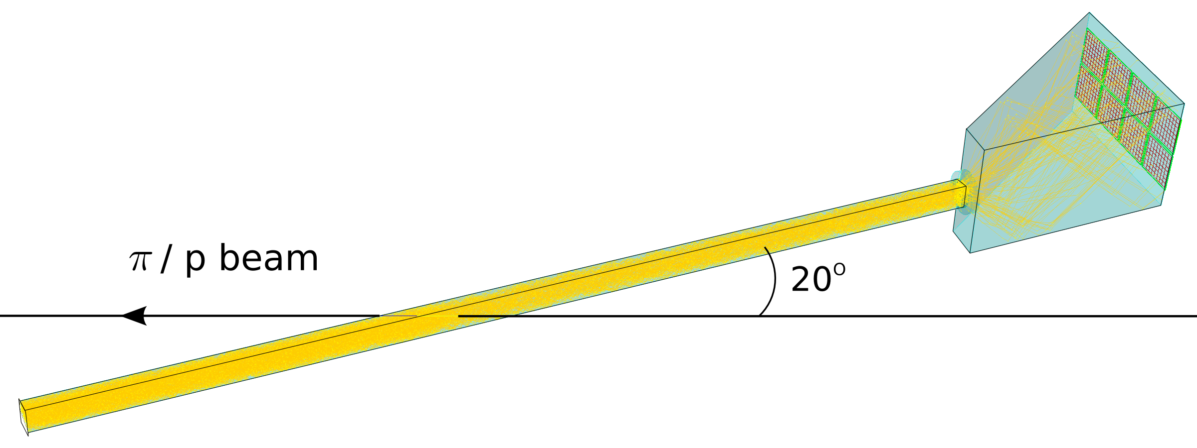
Figure 6: Geant4 simulation of the DIRC prototype configuration at $20^{\circ}$ polar angle. Yellow lines show the path of Cherenkov photons inside the bar and the prism.

The momentum of the mixed hadron beam was set to 7 GeV/c since $\pi/p$ PID challenge at this momenta is equivalent to $\pi/K$’s at 3.5 GeV/c, due to similar Cherenkov angle difference. A time-of-flight system was used to cleanly tag pions and protons.

Figure 7 shows an example of analytical PDFs (solid lines) compared to simulated distributions (shaded histograms) for 30k pions (blue) and protons (red) at $20^{\circ}$ polar angle. The analytical PDFs were obtained with selection constant $w$=0.5 and are in a reasonable agreement with simulation. A slight disagreement in the heights and the positions of the peaks is the result of using idealized geometry for creation of the analytical PDF.

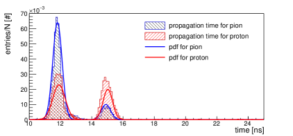
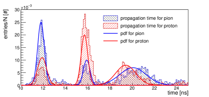
Figure 7: Examples of PDFs for two pixels, number 245 (left) and 285 (right) for pions (blue) and protons (red) at $20^{\circ}$ polar angle and 7 GeV/c momentum. Shaded histograms correspond to the Geant4 simulations for 30k pions and protons while the solid colored lines show analytically determined PDFs.

The resulting likelihood difference distributions of 2k protons and pions are shown in figure 8 for the reconstruction with analytical (left) and simulated (right) PDFs. The time imaging reconstruction with analytical PDFs delivers $4.4\pm 0.1$ s.d. separation which is close to the $4.8\pm 0.1$ s.d. obtained with simulated PDFs. In both cases, the time imaging surpasses the geometrical reconstruction which delivers $4.1\pm 0.1$ s.d.

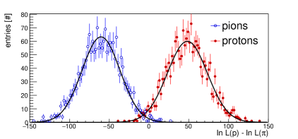
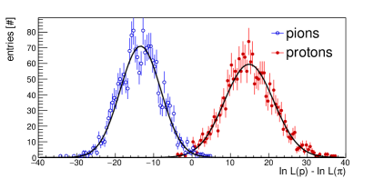
Figure 8: The performance of the time imaging reconstruction for the PANDA Barrel DIRC prototype simulation. The $\pi/p$ log-likelihood difference distributions for pions (blue) and protons (red). The $\pi/p$ separation power from the Gaussian fits is $4.4\pm 0.1$ s.d and $4.8\pm 0.1$ s.d for reconstruction with analytical (left) and simulated (right) PDFs, respectively.

5 Conclusion

The time imaging reconstruction uses both position and time of the detected Cherenkov photons. The photon propagation time distributions are used to construct probability density functions for likelihood calculations. The fastest and most efficient way to create those PDFs is to use analytical calculations. The initial implementation by the Belle II TOP group was extended with look-up-tables to account for the specific focusing system of the PANDA Barrel DIRC. The performance comparison showed that the analytical approach provides a performance close to the best possible one, obtained with simulated PDFs.

References

- [1] PANDA Collaboration, B. Singh et al., Technical Design Report for the PANDA BarrelDIRC Detector, J. Phys. G: Nucl. Part. Phys., 46 045001.
- [2] J. Schwiening et al., The PANDA Barrel DIRC, JINST 13 (2018) C03004.
- [3] PANDA Collaboration, Technical Progress Report, FAIR-ESAC/Pbar (2005).
- [4] R. Dzhygadlo et al., Simulation and reconstruction of the PANDA BarrelDIRC, Nucl. Instr. and Meth. Res. Sect A766 (2014) 263.
- [5] I. Adam et al., The DIRC particle identification system for the BaBar experiment, Nucl. Instr. and Meth. Res. Sect A538 (2005) 281.
- [6] M. Starič et al., Likelihood analysis of patterns in a time-of-propagation (TOP) counter, Nucl. Instr. and Meth. Res. Sect A595 (2008) 252.
- [7] M. Starič, Pattern recognition for the time-of-propagation counter, Nucl. Instr. and Meth. Res. Sect. A639 (2011) 252.
- [8] S. Agostinelli et al., Geant4 - a simulation toolkit, Nucl. Instr. and Meth. Res. Sect. A506 (2003) 250.
- [9] C. Schwarz et al., Status of the PANDA Barrel DIRC, these proceedings.