Coherent States of Systems with
Pure Continuous Energy Spectra

Abstract.

While dealing with a Hamiltonian with continuous spectrum we use a tridiagonal method involving orthogonal polynomials to construct a set of coherent states obeying a Glauber-type condition. We perform a Bayesian decomposition of the weight function of the orthogonality measure to show that the obtained coherent states can be recast in the Gazeau-Klauder approach. The Hamiltonian of the $\ell$-wave free particle is treated as an example to illustrate the method.

1. Introduction

Coherent states (CS) have been introduced by Schrödinger as states which behave in many respects like classical states [1]. They got this name after that Glauber [2] realized that they were particularly convenient to describe optical coherence. In particular, the electromagnetic radiation generated by a classical current is a multimode coherent state, and so is the light produced by a laser in certain regimes [3]. Therefore, CS are cornerstones of modern quantum optics [4] and more recently, CS found applications in quantum information experiments [5].

CS also are mathematical tools which provide a close connection between classical and quantum formalisms so they play a central role in the semiclassical analysis [6, 7].  In general, CS are a specific overcomplete family of vectors in a Hilbert space associated with a quantum mechanical system and can be constructed for that space having either a discrete or continuous basis in different ways [8] : “à la Glauber” as eigenfunctions of an annihilation operator; as states minimizing some uncertainty principle or they can be obtained as orbits of a unitary operator acting on a specific or fiducial state. For the latter one, Weyl defined them for nilpotent groups [9] and this has been extended to Lie groups [10, 11] and further to the continuous spectrum corresponding to the infinite-dimensional unitary representations of noncompact groups [12, 13].

Unlike the case of systems with pure discrete spectrum, constructing CS for a pure continuous spectrum is a challenging problem which may be addressed in different manners but, generally most can be recast in the Gazeau-Klauder CS [14] which were constructed in terms of the energy eigenstates of a given non-degenerate system without referring to any group structure. In [15] a modification allowing to deal with degenerate systems and to treat discrete states and continuous states in a unified way was proposed. The problem of building CS from non-normalizable fiducial states was considered in [16].  In [17] the authors obtained the CS for the continuous spectrum by starting from the hypergeometric CS for the discrete spectrum, and applying a discrete-continuous limit.  In [18], the notion of ladder operators was introduced for systems with continuous spectra together with two kinds of annihilation operators allowing the definition of CS as modified eigenvectors of these operators.

Here, our purpose is to construct, under a Glauber-type condition, a set of CS for a Hamiltonian with continuous spectrum by using the tridiagonal method. We show that this procedure also tells us how to connect the constructed CS with their Gazeau-Klauder version for the Hamiltonian under consideration. This connection is achieved by making appeal to the Bayesian decomposition of the weight function associated with the orthogonal polynomials arising in this method. Indeed, we use the above connection together with the energy eigenstates of the non-degenerate system under consideration to show that we recover the Gazeau-Klauder CS. We illustrate our method for the Hamiltonian of the $l$-wave free particle.

The paper is organized as follows. In section 2, we introduce a set of Glauber-type CS by using a tridiagonal method. In Section 3, we recover the Gazeau-Klauder CS using a Bayesian approach. In Section 4, we illustrate our method for the Hamiltonian of the $\ell$-wave free particle and we discuss some of its properties. Section 5 is devoted to some concluding remarks.

2. Glauber-type CS using the tridiagonal approach

2.1. The tridiagonal approach

Here, we first summarize some needed facts on the tridiagonal method. For this, we assume that the matrix representation of the given Hamiltonian $H$ in a complete orthonormal basis $\mid\phi_{n}>,n=0,1,2,...$ , is tridiagonal. That is,

(2.1) $$\left\langle\phi_{n}\left|H\right|\phi_{m}\right\rangle=b_{n-1}\delta_{n,m+1}+a_{n}\delta_{n,m}+b_{n}\delta_{n,m-1}\text{.}$$

We now define the forward-shift operator $A$ by its action on the basis $\left|\phi_{n}\right\rangle$ as follows

(2.2) $$A\left|\phi_{n}\right\rangle=c_{n}\left|\phi_{n}\right\rangle+d_{n}\left|\phi_{n-1}\right\rangle,\text{ }n=1,2,...\text{ .}$$

For $n=0$, we state that $d_{0}=0.$ Furthermore, we require from the adjoint operator $A^{\dagger}$ to act on the ket vectors $\mid\phi_{n}>$ in the following way:

(2.3) $$A^{\dagger}\left|\phi_{n}\right\rangle=c_{n}\left|\phi_{n}\right\rangle+d_{n+1}\left|\phi_{n+1}\right\rangle\text{, \ \ \ \ \ \ \ \ \ }n=0,1,2,3,...\text{ .}$$

The operator $A^{\dagger}A$ now admits the tridiagonal representation

(2.4) $$\langle\phi_{n}\left|A^{\dagger}A\right|\phi_{m}\rangle=c_{m}d_{m+1}\delta_{n,m+1}+\left(c_{m}c_{m}+d_{m}d_{m}\right)\delta_{n,m}+d_{m}c_{m-1}\delta_{n,m-1}$$

in terms of the coefficients $\left(c_{n},d_{n+1}\right),n=0,1,2,...$ . We have proved [19] that the coefficients in (2.1) are connected to those in $\left(2.2\right)$ by the relations $a_{n}=c_{n}c_{n}+d_{n}d_{n}$ and $b_{n}=c_{n}d_{n+1}$, $n=0,1,2,...$ . The tridiagonal matrix representation of $H$ with respect to the basis $\left|\phi_{n}\right\rangle$ also means that it acts on the elements of this basis as

(2.5) $$H\left|\phi_{n}\right\rangle=b_{n-1}\left|\phi_{n-1}\right\rangle+a_{n}\left|\phi_{n}\right\rangle+b_{n}\left|\phi_{n+1}\right\rangle,\text{ \ }n=0,1,2,...\text{ .}$$

We may then considered the solutions of the eigenvalue problem $H\left|E\right\rangle=E\left|E\right\rangle$ by expanding the eigenvector $\left|E\right\rangle$ in the basis $\left|\phi_{n}\right\rangle$ as

(2.6) $$\left|E\right\rangle=\sum\limits_{n=0}^{+\infty}\mathcal{C}_{n}\left(E\right)\left|\phi_{n}\right\rangle.$$

Then, making use of $\left(2.5\right)$, one readily obtains the following recurrence representation of the expansion coefficients

(2.7) $$E\mathcal{C}_{0}\left(E\right)=a_{0}\mathcal{C}_{0}\left(E\right)+b_{0}\mathcal{C}_{1}\left(E\right),$$

(2.8) $$E\mathcal{C}_{n}\left(E\right)=b_{n-1}\mathcal{C}_{n-1}\left(E\right)+a_{n}\mathcal{C}_{n}\left(E\right)+b_{n}\mathcal{C}_{n+1}\left(E\right),\text{ \ \ \ \ \ }n=1,2,...,$$

and the orthogonality relations

(2.9) $$\delta_{n,m}=\int\limits_{\Omega_{c}}\mathcal{C}_{n}\left(E\right)\mathcal{C}_{m}\left(E\right)dE,\>n,m=1,2,...\text{ .}$$

These relations correspond to the case when the spectrum of the operator $H$ is composed only by a continuous part $\Omega_{c}$. Define

(2.10) $$P_{n}\left(E\right):=\frac{\mathcal{C}_{n}\left(E\right)}{\mathcal{C}_{0}\left(E\right)},\text{ \ }n=0,1,2,...\text{ .}$$

Then $\left\{P_{n}\left(E\right)\right\}$ is a set of polynomials that satisfy the three-term recursion relation for $n\geq 1$

(2.11) $$EP_{n}\left(E\right)=b_{n-1}P_{n-1}\left(E\right)+a_{n}P_{n}\left(E\right)+b_{n}P_{n+1}\left(E\right)$$

with initial conditions $P_{0}\left(E\right)=1$ and $P_{1}\left(E\right)=\left(E-a_{0}\right)b_{0}^{-1}.$ If we now define the density $\omega\left(E\right):=\left(\mathcal{C}_{0}\left(E\right)\right)^{2}$ and assume only existence of continuous spectrum then the relation $\left(2.9\right)$ reads

(2.12) $$\delta_{n,m}=\int\limits_{\Omega_{c}}P_{n}\left(E\right)P_{m}\left(E\right)\omega\left(E\right)dE.$$

Finally, with the help of the above notations, the coefficients $\left(c_{n},d_{n}\right)$ can also be expressed in terms of coefficients $b_{n}$ and the values at zero of consecutive polynomials $\left(P_{n}\right)$ for $n\geq 0$ as 

(2.13) $$\left(d_{n+1}\right)^{2}=-b_{n}\frac{P_{n}\left(0\right)}{P_{n+1}\left(0\right)}\text{ \ \ \ \ \ \ \ \ \ }$$

and

(2.14) $$\left(c_{n}\right)^{2}=-b_{n}\frac{P_{n+1}\left(0\right)}{P_{n}\left(0\right)}\text{.}$$

2.2. Coherent states

As in our previous paper [19] we here adopt the definition of the Glauber-type CS as the eigenstate of the operator $A$ when the Hamiltonian is written as $H=A^{\dagger}A.$  Note that $A$ is here playing the role of annihilation operator. Therefore, we first look to the solution of the eigenproblem

(2.15) $$A\left|\varphi_{z}\right\rangle=z\left|\varphi_{z}\right\rangle$$

with $z$ real. It is not hard to show that the state satisfying $\left(2.15\right)$ has the following representation in the chosen basis $\left|\phi_{n}\right\rangle$ :

(2.16) $$\left|\varphi_{z}\right\rangle=\left(\mathcal{N}\left(z\right)\right)^{-\frac{1}{2}}\sum\limits_{n=0}^{+\infty}Q_{n}\left(z\right)\left|\phi_{n}\right\rangle$$

where

(2.17) $$Q_{n}\left(z\right):=\prod\limits_{j=0}^{n-1}\left(\frac{z-c_{j}}{d_{j+1}}\right),\text{ \ \ }Q_{0}\left(z\right)=1$$

and assuming that

(2.18) $$\mathcal{N}\left(z\right)=\sum\limits_{n=0}^{+\infty}\left|Q_{n}\left(z\right)\right|^{2}<+\infty.$$

For $\left(z,\gamma\right)\in\mathbb{R}^{2}$, the generalized CS associated to $H$ are defined as the orbit of the evolution semigroup $e^{-i\gamma H}$ while acting on the fiducial state $\left|\varphi_{z}\right\rangle.$ That is,

(2.19) $$\left|z,\gamma\right\rangle=e^{-i\gamma H}\left|\varphi_{z}\right\rangle.$$

Note that $\gamma$ can be interpreted as a time parameter.  One observes from $\left(2.17\right)$ that when $z=c_{k}$ then the series $\left(2.16\right)$ terminates and the coherent states reduce to

(2.20) $$\left|c_{k},\gamma\right\rangle=\left(\mathcal{N}\left(c_{k}\right)\right)^{-\frac{1}{2}}\sum\limits_{n=0}^{k}Q_{n}\left(c_{k}\right)e^{-i\gamma H}\left|\phi_{n}\right\rangle.$$

We may also write the $\left|\phi_{n}\right\rangle$ as

(2.21) $$\left|\phi_{n}\right\rangle=\int\limits_{0}^{+\infty}\left|E\right\rangle\sqrt{\omega\left(E\right)}P_{n}\left(E\right)dE$$

which leads to

(2.22) $$e^{-i\gamma H}\left|\phi_{n}\right\rangle=\int\limits_{0}^{+\infty}e^{-i\gamma H}\left|E\right\rangle\sqrt{\omega\left(E\right)}P_{n}\left(E\right)dE.$$

We use the fact that

(2.23) $$e^{-i\gamma H}\left|E\right\rangle=e^{-i\gamma E}\left|E\right\rangle$$

gives

(2.24) $$e^{-i\gamma H}\left|\phi_{n}\right\rangle=\int\limits_{0}^{+\infty}\left|E\right\rangle\sqrt{\omega\left(E\right)}P_{n}\left(E\right)e^{-i\gamma E}dE.$$

Recall that

(2.25) $$\langle r\left|E\right\rangle=\sqrt{\omega\left(E\right)}\sum\limits_{j=0}^{+\infty}P_{j}\left(E\right)\phi_{j}\left(r\right).$$

Therefore,

(2.26) $$\langle r\left|e^{-i\gamma H}\right|\phi_{n}\rangle=\int\limits_{0}^{+\infty}e^{-i\gamma E}\left[\sum\limits_{j=0}^{+\infty}\phi_{j}\left(r\right)P_{j}\left(E\right)\right]\omega\left(E\right)P_{n}\left(E\right)dE$$

(2.27) $$=\int\limits_{0}^{+\infty}\mathcal{K}\left(r,y\right)P_{n}\left(y\right)\omega\left(y\right)e^{-i\gamma y}dy$$

where

(2.28) $$\mathcal{K}\left(x,y\right):=\sum\limits_{j=0}^{+\infty}\phi_{j}\left(x\right)P_{j}\left(y\right).$$

Finally, summarizing the above calculations, the wave function in Eq.$\left(2.20\right)$ may also be presented in an integral form as

(2.29) $$\langle r\left|c_{k},\gamma\right\rangle=\left(\mathcal{N}\left(c_{k}\right)\right)^{-\frac{1}{2}}\int\limits_{0}^{+\infty}\mathcal{K}\left(r,y\right)\mathcal{S}\left(c_{k},y\right)\omega\left(y\right)e^{-i\gamma y}dy$$

where

(2.30) $$\mathcal{S}\left(u,y\right):=\sum_{n=0}^{k}Q_{n}\left(u\right)P_{n}\left(y\right).$$

3. Deducing Gazeau-Klauder CS using a Bayesian analysis

3.1. Bayesian analysis

Here, our goal is the deduce the Gazeau-Klauder CS [14] from the above constructed ones $\left(2.29\right)$. For that, we assume that the weight function $\omega_{\lambda}\left(E\right)$ associated with orthogonal polynomials $\left\{P_{n}\left(E\right)\right\}$ depends on a parameter $\lambda$ and that it’s a density function for a probability distribution. Now, the question is to determine two functions: $E\mapsto q\left(E\right)$ and the other $\lambda\mapsto\tau\left(\lambda\right)$ that may enter in the following decomposition

(3.1) $$\frac{\left(\tau\left(\lambda\right)\right)^{2E}q\left(E\right)}{\int\left(\tau\left(\lambda\right)\right)^{2y}q\left(y\right)dy}=\omega_{\lambda}\left(E\right).$$

For that we may look at this problem from a Bayesian viewpoint by saying that $\left(3.1\right)$ also means that the weight function

(3.2) $$\omega_{\lambda}\left(E\right)\equiv\pi\left(E\rfloor\lambda\right)$$

can be considered as a posterior distribution (or inverse) for an unknown distribution denoted here by $\pi\left(\eta\rfloor E\right)$ where $E$ may play the role of a parameter and $\eta$ denotes the variable or the observed data. We say that $\pi\left(\eta\rfloor E\right)$ is the statistical model. Also from $\left(3.1\right)$, the unknown quantity $\left(\tau\left(\lambda\right)\right)^{2E}$  may play the role of a prior distribution on the parameter $E$ which itself is modeled as a random variable. That is,

(3.3) $$\left(\tau\left(\lambda\right)\right)^{2E}\equiv\pi_{\lambda}\left(E\right)$$

called the prior. According to the general basic definition ([20], pp.8-10) we also say that $\pi\left(E\rfloor\lambda\right)$ the posterior are conjugate under $\pi\left(\eta\rfloor E\right)$ the model. Doing so, our problem in $\left(3.1\right)$, can be formulated as follows : given $\omega_{\lambda}\left(E\right)\equiv\pi\left(E\rfloor\lambda\right)$ as posterior, we may ask under which model $\pi\left(\eta\rfloor E\right)\equiv q\left(E\right)$ the probability law defined by $\omega_{\lambda}\left(E\right)$ could be conjugate to some prior $\pi_{\lambda}\left(E\right)$ to be determined ?.

Finally, in concrete situations one will be dealing with the weight function $\omega_{\lambda}\left(E\right)$ will be given explicitly therefore we can find the two quantities $q\left(E\right)$ and $\tau\left(\lambda\right)$. The latter ones, can be used to prove that the constructed CS we have introduced via the tridiagonal method procedure agree with the Gazeau-Klauder CS for the continuous spectrum. Indeed, as we will see below this analysis will provide us with the factorial function $f\left(E\right)$ and the re-parametrization formula $s=\tau\left(\lambda\right)$ that serve as a bridge linking the two approaches.

3.2. Gazeau-Klauder CS

Let  $H>0$ be a Hamiltonian operator with non-degenerate continuous spectrum and let $\left\{\left|E\right\rangle\right\}$ stands for a basis of eigenstates in some Hilbert space $\mathcal{H}$, for which

(3.4) $$H\left|E\right\rangle=E\left|E\right\rangle,\text{ \ \ \ }0<E<\overline{E}$$

so that the energy support is $\left[0,\overline{E}\right).$ Here $\overline{E}=+\infty$ could be considered. We also can choose a normalized basis of eigenvectors of $\mathcal{H}$ :

(3.5) $$\langle E\left|E^{\prime}\right\rangle=\delta\left(E-E^{\prime}\right)$$

and

(3.6) $$\int\limits_{0}^{\overline{E}}\left|E\right\rangle\left\langle E\right|dE=\mathbf{1}_{\mathcal{H}}.$$

For $s\geq 0$ and $\gamma\in\mathbb{R}$, the Gazeau-Klauder CS [14] are defined by

(3.7) $$\left|s,\gamma\right\rangle=\left(\mathcal{N}\left(s\right)\right)^{-\frac{1}{2}}\int\limits_{0}^{\overline{E}}\frac{s^{E}}{\sqrt{f\left(E\right)}}e^{-i\gamma E}\left|E\right\rangle dE.$$

These states are normalized

(3.8) $$\langle s,\gamma\left|s,\gamma\right\rangle=1$$

and

(3.9) $$\mathcal{N}\left(s\right)=\int_{0}^{\overline{E}}\frac{s^{2E}}{f\left(E\right)}dE$$

is a normalization factor. The function $E\mapsto f(E)$ is determined by a suitable non-negative weight function $\sigma(s)\geq 0$ as

(3.10) $$f(E)=\int\limits_{0}^{\overline{E}}s^{2E}\sigma(s)ds.$$

With the measure

(3.11) $$d\mu(s,\gamma)=\frac{1}{2\pi}\mathcal{N}(s)\sigma(s)dsd\gamma,$$

the resolution of the identity reads

(3.12) $$\int\left|s,\gamma\right\rangle\left\langle s,\gamma\right|d\mu\left(s,\gamma\right)=\mathbf{1}_{\mathcal{H}}.$$

Finally, from the above Bayesian decomposition of $\omega_{\lambda}\left(E\right),$ we choose $f(E)$ to be the inverse of $q\left(E\right)$, i.e.,

(3.13) $$f\left(E\right)\equiv\frac{1}{q\left(E\right)}$$

and we take

(3.14) $$s\equiv\tau\left(\lambda\right)$$

as a new parametrization.

4. Coherent states associated with the $\ell$-wave free particle 

We start with separating the angular part of the wavefunction of the free particle in terms of the spherical harmonics that are eigenfunctions of the angular momentum which is conserved for this kind of potentials. That leaves for the radial part of the wavefunction the Schrödinger operator

(4.1) $$H_{\ell}:=-\frac{1}{2}\frac{d^{2}}{dr^{2}}+\frac{1}{2}\frac{\ell\left(\ell+1\right)}{r^{2}}$$

which acts on the Hilbert space $\mathcal{H}:=L^{2}\left(\mathbb{R}_{+},dr\right)$ and admits a continuous spectrum $E\in\left[0,+\infty\right)$. Hence it is positive semi-definite. Here, the oscillator space $\mathcal{H}$ is endowed with the orthonormal basis whose elements are given by

(4.2) $$\phi_{n}^{(\ell,\lambda)}\left(r\right):=\sqrt{\frac{2\lambda n!}{\Gamma\left(n+\ell+\frac{3}{2}\right)}}\left(\lambda r\right)^{\ell+1}\exp\left(-\frac{\lambda^{2}}{2}r^{2}\right)L_{n}^{\left(\ell+\frac{1}{2}\right)}\left(\lambda^{2}r^{2}\right),\text{ \ }n=0,1,2,...,$$

$r\in\mathbb{R}_{+}$ where $\lambda$ denotes a real free parameter, $\ell$ is the angular momentum number and $L_{n}^{\left(\sigma\right)}\left(.\right)$ is the Laguerre polynomial ([21], p.1000). Using differential recurrence relations for these polynomials, one finds by direct calculations that the matrix elements defined by

(4.1) $$\langle\phi_{n}^{(\ell,\lambda)}\left|H_{\ell}\right|\phi_{m}^{(\ell,\lambda)}\rangle=\int\limits_{0}^{+\infty}\phi_{n}^{(\ell,\lambda)}\left(r\right)H\left[\phi_{m}^{(\ell,\lambda)}\right]\left(r\right)dr$$

have the following expression

(4.3) $$\langle\phi_{n}^{(\ell,\lambda)}\left|H_{\ell}\right|\phi_{m}^{(\ell,\lambda)}\rangle=\frac{\lambda^{2}}{2}\left(2n+\ell+\frac{3}{2}\right)\delta_{n,m}+\frac{\lambda^{2}}{2}\sqrt{n\left(n+\ell+\frac{3}{2}\right)}\delta_{n,m+1}$$

$$+\frac{\lambda^{2}}{2}\sqrt{\left(n+1\right)\left(n+\ell+\frac{3}{2}\right)}\delta_{n,m-1}.$$

Therefore, we can identify the coefficients $\left(a_{n}\right)$ and $\left(b_{n}\right)$ in $\left(2.1\right)$ as follows

(4.4a) $$a_{n}=\frac{\lambda^{2}}{2}\left(2n+\ell+\frac{3}{2}\right),$$

(4.4b) $$b_{n}=\frac{\lambda^{2}}{2}\sqrt{\left(n+1\right)\left(n+\ell+\frac{3}{2}\right)}.$$

According to equation $\left(4.3\right)$, the recursion relation is solved,

(4.5) $$P_{n}\left(E\right)=\left(-1\right)^{n}\sqrt{\frac{n!\Gamma\left(\ell+\frac{3}{2}\right)}{\Gamma\left(n+\ell+\frac{3}{2}\right)}}L_{n}^{\left(\ell+\frac{1}{2}\right)}\left(\frac{2}{\lambda^{2}}E\right).$$

These polynomials satisfy the orthogonality relations

(4.6) $$\int\limits_{0}^{+\infty}P_{j}\left(E\right)P_{k}\left(E\right)\omega_{\ell,\lambda}\left(E\right)dE=\delta_{j,k}$$

with respect to the weight function

(4.7) $$\omega_{\ell,\lambda}\left(E\right)=\frac{2}{\lambda^{2}\Gamma\left(\ell+\frac{3}{2}\right)}\left(\frac{2}{\lambda^{2}}E\right)^{\ell+\frac{1}{2}}\exp\left(-\frac{2}{\lambda^{2}}E\right).$$

Note that $\omega_{\ell,\lambda}\left(E\right)$ is the continuous density function of the Gamma probability distribution $G\left(\alpha,\beta\right)$ with the shape parameter $\alpha=\ell+\frac{3}{2}$ and the scale parameter $\beta=2\lambda^{-2}.$ Finally, with

(4.8) $$P_{n}\left(0\right)=\left(-1\right)^{n}\sqrt{\frac{\Gamma\left(n+\ell+\frac{3}{2}\right)}{n!\Gamma\left(\ell+\frac{3}{2}\right)}}$$

equations $\left(2.13\right),\left(2.14\right)$ together with $\left(3.20\right)$ yield

(4.9) $$d_{n+1}=\frac{\lambda}{\sqrt{2}}\sqrt{n+1},\text{ \ }c_{n}=\frac{\lambda}{\sqrt{2}}\sqrt{n+\ell+\frac{3}{2}}.$$

The kernel function $\mathcal{K}$ in $\left(2.28\right)$ has the form

(4.10) $$\mathcal{K}\left(r,E\right)=\sum\limits_{j=0}^{+\infty}\phi_{j}^{(\ell,\lambda)}\left(r\right)P_{j}\left(E\right)$$

(4.2) $$=\left(\lambda r\right)^{\ell+1}e^{-\frac{1}{2}\left(\lambda r\right)^{2}}\sqrt{2\lambda\Gamma\left(\ell+\frac{1}{2}\right)}\sum\limits_{j=0}^{+\infty}\frac{j!\left(-1\right)^{j}}{\Gamma\left(j+\ell+\frac{3}{2}\right)}L_{j}^{\left(\ell+\frac{1}{2}\right)}\left(\left(\lambda r\right)^{2}\right)L_{j}^{\left(\ell+\frac{1}{2}\right)}\left(\frac{2E}{\lambda^{2}}\right).$$

We now make use of the formula

(4.11) $$\sum\limits_{j=0}^{+\infty}\frac{j!\left(-h\right)^{j}}{\Gamma\left(j+\nu+1\right)}\left(-h\right)^{j}L_{j}^{\left(\nu\right)}\left(x\right)L_{j}^{\left(\nu\right)}\left(y\right)=\frac{e^{\left(x+y\right)\frac{h}{1+h}}}{1+h}\left(xyh\right)^{-\frac{\nu}{2}}J_{\nu}\left(2\sqrt{xy}\frac{h^{\frac{1}{2}}}{1+h}\right)$$

(see [23], p.139, (12a) and p.140 for $h\rightarrow 1)$ for $\nu=\ell+\frac{1}{2}$, $x=\lambda^{2}r^{2}$ and $y=2\lambda^{-2}E,$ we get that

(4.12) $$\mathcal{K}\left(r,E\right)=\frac{1}{2}\lambda^{\ell+1}r^{\frac{1}{2}}\sqrt{2\lambda\Gamma\left(\ell+\frac{1}{2}\right)}e^{\lambda^{-2}E}\left(2E\right)^{-\frac{1}{2}\left(\ell+\frac{1}{2}\right)}J_{\ell+\frac{1}{2}}\left(\sqrt{2r^{2}E}\right).$$

We also need to specify the kernel function $\mathcal{S}$ defined in $\left(2.30\right):$

(4.13) $$\mathcal{S}\left(c_{k},y\right):=\sum_{n=0}^{k}Q_{n}\left(c_{k}\right)P_{n}\left(y\right)=\sum_{n=0}^{k}\prod\limits_{j=0}^{n-1}\left(\frac{c_{k}-c_{j}}{d_{j+1}}\right)P_{n}\left(y\right).$$

Therefore,

(4.14) $$\langle r\left|c_{k},\gamma\right\rangle=\left(\mathcal{N}\left(c_{k}\right)\right)^{-\frac{1}{2}}\sum_{n=0}^{k}\prod\limits_{j=0}^{n-1}\left(\frac{c_{k}-c_{j}}{d_{j+1}}\right)\int\limits_{0}^{+\infty}\mathcal{K}\left(r,y\right)P_{n}\left(y\right)\omega_{\lambda,\ell}\left(y\right)e^{-i\gamma y}dy.$$

The integral in $\left(4.14\right)$ reads

$$\int\limits_{0}^{+\infty}\mathcal{K}\left(r,y\right)P_{n}\left(y\right)\varrho\left(y\right)e^{-i\gamma y}dy=\frac{\left(-1\right)^{n}\lambda^{-\ell-\frac{3}{2}}}{\left(\ell+\frac{1}{2}\right)}\sqrt{\frac{2n!}{\Gamma\left(n+\ell+\frac{3}{2}\right)}}r^{\frac{1}{2}}2^{\frac{1}{2}\left(\ell+\frac{1}{2}\right)}$$

(4.15) $$\times\int\limits_{0}^{+\infty}e^{-\frac{1}{\lambda^{2}}y}y^{\frac{1}{2}\left(\ell+\frac{1}{2}\right)}J_{\ell+\frac{1}{2}}\left(\sqrt{2r^{2}y}\right)L_{n}^{\left(\ell+\frac{1}{2}\right)}\left(\frac{2}{\lambda^{2}}y\right)e^{-i\gamma y}dy.$$

For $k=0$ formula $\left(4.14\right)$ reduces to

(4.16) $$\langle r\left|c_{0},\gamma\right\rangle=\left(\mathcal{N}\left(c_{0}\right)\right)^{-\frac{1}{2}}\int\limits_{0}^{+\infty}\mathcal{K}\left(r,y\right)\omega_{\lambda,\ell}\left(y\right)e^{-i\gamma y}dy$$

$$=\left(\mathcal{N}\left(c_{0}\right)\right)^{-\frac{1}{2}}\frac{1}{2}\lambda^{\ell+1}r^{\frac{1}{2}}\sqrt{2\lambda\Gamma\left(\ell+\frac{1}{2}\right)}\frac{2}{\lambda^{2}}\frac{1}{\Gamma\left(\ell+\frac{3}{2}\right)}2^{-\frac{1}{2}\left(\ell+\frac{1}{2}\right)}\left(\frac{2}{\lambda^{2}}\right)^{\frac{1}{2}+\ell}$$

(4.17) $$\times\int\limits_{0}^{+\infty}y^{\frac{1}{2}\left(\ell+\frac{1}{2}\right)}J_{\ell+\frac{1}{2}}\left(\sqrt{2r^{2}y}\right)e^{-\frac{1}{\lambda^{2}}y}e^{-i\gamma y}dy.$$

By the variable change $y=x^{2},$ the last integral becomes

(4.18) $$2\int\limits_{0}^{+\infty}x^{\left(\ell+\frac{1}{2}\right)+1}J_{\ell+\frac{1}{2}}\left(\sqrt{2r^{2}}x\right)e^{-(\frac{1}{\lambda^{2}}+i\gamma)x^{2}}dx.$$

Next, by using the identity ([21], p.706)

(4.19) $$\int\limits_{0}^{+\infty}x^{\nu+1}e^{-\alpha x^{2}}J_{\nu}\left(\beta x\right)dx=\frac{\beta^{\nu}}{\left(2\alpha\right)^{\nu+1}}\exp\left(-\frac{\beta^{2}}{4\alpha}\right),\text{ \ \ }\mathop{\mathrm{R}e}\alpha>0,\mathop{\mathrm{R}e}\nu>-1,$$

for $\beta=\sqrt{2r^{2}},\nu=\left(\ell+\frac{1}{2}\right)$ and $\alpha=(\frac{1}{\lambda^{2}}+i\gamma)$, we arrive at the expression

(4.20) $$\langle r\left|\lambda,\gamma\right\rangle=\sqrt{2}\left(\Gamma\left(\ell+\frac{3}{2}\right)\right)^{-\frac{1}{2}}\left(\frac{1}{\lambda}\right)^{\left(\ell+\frac{3}{2}\right)}\frac{r^{\ell+1}}{\left(\frac{1}{\lambda^{2}}+i\gamma\right)^{\ell+\frac{3}{2}}}\exp\left(-\frac{r^{2}}{2(\frac{1}{\lambda^{2}}+i\gamma)}\right).$$

Note that with respect to the basis $\left(4.2\right)$ one can observe that the coefficient $c_{0}$ in $\left(4.16\right)$ coincides with the labeling parameter $z$ according to calculations that start by the formula $\left(2.16\right).$ So the above equation $\left(4.20\right)$ represents in fact the wave function in $r-$coordinate of a coherent state with the given $z$ provided we choose the value $\lambda=\frac{2}{\sqrt{2l+3}}z.$

Now, for a Bayesian decomposition of the weight function purpose, we first observe that $\omega_{\lambda,\ell}\left(E\right)$ as given by $\left(4.7\right)$ is a Gamma distribution $\mathcal{G}\left(\ell+\frac{3}{2},\frac{2}{\lambda^{2}}\right).$ It is also well known that for the Poisson model $X\sim\mathcal{P}\left(\kappa\right)$ with $\kappa>0$ given by the probability distribution

(4.21) $$\Pr\left(X=j\right)=\frac{\kappa^{j}}{j!}e^{-\kappa},\text{ }j=0,1,2,...,$$

if the prior distribution on the parameter $\kappa$ is a Gamma distribution $\mathcal{G}\left(\alpha,\beta\right)$ then the posterior distribution is also a Gamma distribution $\mathcal{G}\left(\alpha+j,\beta+1\right).$ Thus, in terms of our notations,

(4.22) $$\Pr\left(X=\ell\right)=\frac{E^{\ell}}{\ell!}e^{-E}\equiv p_{E}\left(l\right),\text{ }l=0,1,2,...,\text{ }E>0\text{\ }$$

where $X\sim\mathcal{P}\left(E\right),$ is a convenient statistical model. This also indicates that the angular momentum integer number $l$ may in fact play the role of an observed data of a discrete random variable  $X\sim\mathcal{P}\left(E\right)$ with the energy $E>0$ as its parameter. Therefore, we now fixe $l$ and proceed to reverse $X$ by fixing ”à priori” a law $\pi_{\lambda}\left(E\right)$ that $E$ is supposed to follow. The prior law on the prameter can be obtained just by writting our weight function $\omega_{\lambda,\ell}\left(E\right)\equiv\mathcal{G}\left(\ell+\frac{3}{2},\frac{2}{\lambda^{2}}\right)$ as a gamma distribution $\mathcal{G}\left(\alpha+\ell,\beta+1\right).$This gives us

(4.23) $$\pi_{\lambda}\left(E\right):=\mathcal{G}\left(\frac{3}{2},\frac{2}{\lambda^{2}}-1\right)$$

and therefor we can rewrite the weight function as a posterior distribution as

(4.24) $$\frac{\left[\pi_{\lambda}\left(E\right)\right]\left[p_{E}\left(\ell\right)\right]}{\int\left[\pi_{\lambda}\left(y\right)\right]\left[p_{y}\left(\ell\right)\right]dy}=\omega_{\lambda,l}\left(E\right),$$

which, after simplification, reduces to

(4.25) $$\frac{\left[e^{-\frac{2}{\lambda^{2}}E}\right]\left[E^{\frac{1}{2}+\ell}\right]}{\int\limits_{0}^{+\infty}y^{\frac{1}{2}+\ell}e^{-\frac{2}{\lambda^{2}}y}dy}=\omega_{\lambda,\ell}\left(E\right).$$

In other words,

(4.26) $$\omega_{\lambda,l}\left(E\right)\propto\left(\tau\left(\lambda\right)\right)^{2E}q\left(E\right)$$

where

(4.27) $$\tau\left(\lambda\right)=e^{-\frac{1}{\lambda^{2}}}$$

and

(4.27) $$q\left(E\right)=E^{\frac{1}{2}+l}.$$

Now, in order to recover the constructed CS in $\left(4.20\right)$ by the Gazeau-Klauder formalism let us recall that the operator $H_{\ell}$ acts on the Hilbert space $L^{2}\left(\mathbb{R}_{+},dr\right)$ and admits a continous spectrum $E\in\left[0,+\infty\right)$. The Schrödinger equation $H_{\ell}\varphi=E\varphi$ has a regular solution given by

(4.28) $$\hat{\jmath}_{\ell}\left(kr\right)=\sqrt{kr}J_{\ell+\frac{1}{2}}\left(kr\right),\text{ \ }$$

where $J_{\nu}$ denotes the Bessel function of the first kind and of order $\nu$ ([21], p.910) and $k=\sqrt{2E}$. The function $\hat{\jmath}_{\ell}$ is regular for $r\rightarrow 0$ for $\ell>0.$ Therefore, eigenstates are those given by

(4.29) $$\langle r\left|E\right\rangle=\sqrt{kr}J_{\ell+\frac{1}{2}}\left(kr\right).$$

From the above Bayesian decomposition of the weight function $\omega_{\ell,\lambda}\left(E\right)$ we choose the factorial function to be defined by

(4.30) $$f_{\ell}\left(E\right):=\frac{1}{q\left(E\right)}=\left(2E\right)^{-\left(\frac{1}{2}+\ell\right)}.$$

Therefore, the corresponding Steiljes moment problem

(4.31) $$f_{l}(E)=\int\limits_{0}^{+\infty}s^{2E}\sigma(s)ds$$

can be solved by the weight function

(4.32) $$\sigma_{\ell}\left(s\right)=\frac{1}{\Gamma\left(\frac{1}{2}+\ell\right)}\frac{1}{s}\left(Log\frac{1}{s}\right)^{-\frac{1}{2}+\ell},\text{ }s<1$$

and $\sigma_{\ell}\left(s\right)=0$ for $s\geq 1,$ by making appeal to the Mellin transform ([22], p.343) :

(4.33) $$\int\limits_{0}^{+\infty}\phi_{\alpha,\nu}\left(x\right)x^{p-1}dx=\Gamma\left(\nu\right)\left(p+1\right)^{-\nu},\mathop{\mathrm{R}e}\nu>0,\mathop{\mathrm{R}e}p>-\mathop{\mathrm{R}e}\alpha,$$

where $\phi_{\alpha,\nu}\left(x\right)=x^{\alpha}\left(-Logx\right)^{\nu-1}$, $0<x<1$ and $\phi_{\alpha,\nu}\left(x\right)=0$, $x\in\left[1,+\infty\right),$ for $p=2E+1,\nu=\frac{1}{2}+\ell$ and $\alpha=-1$. Therefore, the normalization factor $\left(2.3\right)$, here,

(4.34) $$\mathcal{N}_{\ell}\left(s\right)=\frac{1}{2}\Gamma\left(\frac{3}{2}+\ell\right)\left(Log\frac{1}{s}\right)^{-\left(\frac{3}{2}+\ell\right)}.$$

With these ingredients, the CS $\left(3.7\right)$ take the form

(4.35) $$\left|s,\gamma\right\rangle=\left(\mathcal{N}_{\ell}\left(s\right)\right)^{-\frac{1}{2}}\int\limits_{0}^{+\infty}dE\frac{s^{E}e^{-i\gamma E}}{\sqrt{\left(2E\right)^{-\left(\frac{1}{2}+\ell\right)}}}\left|E\right\rangle.$$

Now, from the above Bayesian decomposition of $\omega_{\ell,\lambda}\left(E\right)$ we choose the following reparametrization for the labeling parameter $s$ according to $\left(4.27\right)$ as

(4.36) $$s=\tau\left(\lambda\right)=\exp\left(-\frac{1}{\lambda^{2}}\right),\text{ \ }0\leq s<1,\text{ \ }\lambda\in\mathbb{R},$$

then $\left(4.18\right)$ takes the form

(4.37) $$\left|\lambda,\gamma\right\rangle=\left(\mathcal{N}_{l}\left(s\right)\right)^{-\frac{1}{2}}\int\limits_{0}^{+\infty}\frac{e^{-(\frac{1}{\lambda^{2}}+i\gamma)E}}{\sqrt{\left(2E\right)^{-\left(\frac{1}{2}+\ell\right)}}}\left|E\right\rangle dE.$$

Next, making use of $\left(4.29\right)$, we obtain successively

(4.38) $$\langle r\left|\lambda,\gamma\right\rangle=\left(\mathcal{N}_{l}\left(s\right)\right)^{-\frac{1}{2}}\int\limits_{0}^{+\infty}\left(2E\right)^{\frac{1}{2}\left(\frac{1}{2}+l\right)}e^{-(\frac{1}{\lambda^{2}}+i\gamma)E}\left[\sqrt{r}J_{l+\frac{1}{2}}\left(kr\right)\right]dE$$

(4.39) $$=\sqrt{r}\left(\mathcal{N}_{l}\left(s\right)\right)^{-\frac{1}{2}}\int\limits_{0}^{+\infty}\sqrt{2E}^{\left(\frac{1}{2}+l\right)}e^{-\frac{1}{2}(\frac{1}{\lambda^{2}}+i\gamma)\left(\sqrt{2E}\right)^{2}}J_{l+\frac{1}{2}}\left(\sqrt{2E}r\right)dE$$

(4.40) $$=\sqrt{r}\left(\mathcal{N}_{l}\left(s\right)\right)^{-\frac{1}{2}}\int\limits_{0}^{+\infty}x^{(\frac{1}{2}+l)+1}e^{-\frac{1}{2}(\frac{1}{\lambda^{2}}+i\gamma)x^{2}}J_{l+\frac{1}{2}}\left(xr\right)dx.$$

By applying the formula ([21], p.706):

(4.41) $$\int\limits_{0}^{+\infty}x^{\nu+1}e^{-\alpha x^{2}}J_{\nu}\left(\beta x\right)dx=\frac{\beta^{\nu}}{\left(2\alpha\right)^{\nu+1}}\exp\left(-\frac{\beta^{2}}{4\alpha}\right),\text{ \ \ }\mathop{\mathrm{R}e}\alpha>0,\mathop{\mathrm{R}e}\nu>-1,$$

for parameters $\nu=l+\frac{1}{2},$ $\alpha=\frac{1}{2}(\frac{1}{\lambda^{2}}+i\gamma)$ and $\beta=r$, Eq. $\left(4.40\right)$ reads

(4.42) $$\langle r\left|\lambda,\gamma\right\rangle=\left(\mathcal{N}_{l}\left(s\right)\right)^{-\frac{1}{2}}\frac{r^{l+1}}{\left(\frac{1}{\lambda^{2}}+i\gamma\right)^{l+\frac{1}{2}+1}}\exp\left(-\frac{r^{2}}{2(\frac{1}{\lambda^{2}}+i\gamma)}\right).$$

Finally, we replace $\mathcal{N}_{l}\left(s\right)$ by is expression $\left(4.34\right)$ to arrive at the expression

(4.43) $$\langle r\left|\lambda,\gamma\right\rangle=\sqrt{2}\left(\Gamma\left(l+\frac{3}{2}\right)\right)^{-\frac{1}{2}}\left(\frac{1}{\lambda}\right)^{\left(l+\frac{3}{2}\right)}\frac{r^{l+1}}{\left(\frac{1}{\lambda^{2}}+i\gamma\right)^{l+\frac{3}{2}}}\exp\left(-\frac{r^{2}}{2(\frac{1}{\lambda^{2}}+i\gamma)}\right).$$

The above expression of coherent states $\left(4.42\right)$ is a major result. It has the following properties. For $\gamma=0,$ the corresponding expression of CS reduces to

(4.44) $$\langle r\left|\lambda,0\right\rangle=\sqrt{\frac{2\lambda}{\Gamma\left(\ell+\frac{3}{2}\right)}}(\lambda r)^{l+1}\exp\left(-\frac{\lambda^{2}}{2}r^{2}\right).$$

Recall that for the basis vectors $\phi_{n}^{(\ell,\lambda)}\left(r\right)$ in $\left(4.2\right)$ we have for $n=0$

(4.45) $$\phi_{0}^{(\ell,\lambda)}\left(r\right):=\sqrt{\frac{2\lambda}{\Gamma\left(\ell+\frac{3}{2}\right)}}\left(\lambda r\right)^{\ell+1}\exp\left(-\frac{\lambda^{2}}{2}r^{2}\right).$$

So we may rewrite $\left(4.44\right)$ as $\langle r\left|\lambda,0\right\rangle=\phi_{0}^{(\ell,\lambda)}\left(r\right)$ as expected. The combined energy exponential in the integral in $\left(4.37\right)$ is now

(4.46) $$e^{-\frac{1}{\beta^{2}}E},\text{ \ \ \ }\frac{1}{\beta^{2}}=\frac{1}{\lambda^{2}}+i\gamma.$$

We therefore have the result

(4.47) $$\langle r\left|\lambda,\gamma\right\rangle=\left(\frac{\beta}{\lambda}\right)^{\ell+\frac{3}{2}}\phi_{0}^{(\ell,\beta)}\left(r\right).$$

Explicitly, we have the density function

(4.48) $$\rho\left(r;\lambda,\gamma\right):=\left|\langle r\left|\lambda,\gamma\right\rangle\right|^{2}=\frac{2\lambda^{2l+3}}{\Gamma\left(l+\frac{3}{2}\right)(1+\gamma^{2}\lambda^{4})^{l+3/2}}\;r^{2l+2}e^{\frac{-r^{2}\lambda^{2}}{1+\lambda^{4}\gamma^{2}}}.$$

In figure 1, we show the behavior of the function $r\mapsto\rho\left(r;\lambda,\gamma\right)$ for several discrete values of $\gamma.$

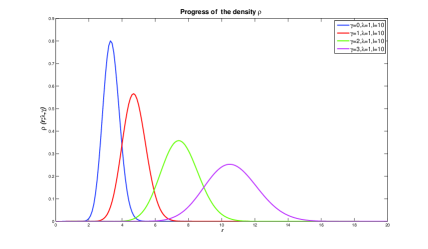
Figure 1. $r\mapsto\rho\left(r;\lambda,\gamma\right)$ for several discrete values of $\gamma.$

We now can calculate the average position

(4.49) $$\overline{r}\left(\gamma\right):=\int\limits_{0}^{+\infty}r\rho\left(r;\lambda,\gamma\right)dr=\frac{2\lambda^{2l+3}}{\Gamma\left(l+\frac{3}{2}\right)(1+\gamma^{2}\lambda^{4})^{l+3/2}}\int\limits_{0}^{+\infty}e^{\frac{r^{2}}{\lambda^{2}\gamma^{2}-\lambda^{-2}}}r^{2l+3}dr.$$

Applying the integral ([21], p.337):

(4.50) $$\int\limits_{0}^{+\infty}x^{m}e^{-\beta x^{n}}dx=\frac{1}{n\beta^{\frac{m+1}{n}}}\Gamma(\frac{m+1}{n}),\text{ \ }\mathop{\mathrm{R}e}m>0,\,\mathop{\mathrm{R}e}\,n>0,\,\mathop{\mathrm{R}e}\beta>0$$

for $m=2l+3$, $n=2$ and $\beta=\frac{\lambda^{2}}{1+\lambda^{4}\gamma^{2}}$, Eq.$\left(4.49\right)$ takes the form

(4.51) $$\overline{r}\left(\gamma\right)=C\frac{(l+1)!}{\Gamma\left(l+3/2\right)}\left(\frac{1}{\lambda^{2}}+\lambda^{2}\gamma^{2}\right)^{1/2}.$$

Note that when $l=0$, the average position reduces to $\frac{2}{\sqrt{\pi}}\left(\frac{1}{\lambda^{2}}+\lambda^{2}\gamma^{2}\right)^{1/2}$. On other hand the velocity (with respect to $\gamma)$ is

$$\upsilon\left(\gamma\right):=\partial_{\gamma}\left(\overline{r}\left(\gamma\right)\right)=\frac{(l+1)!}{\Gamma\left(l+3/2\right)}\frac{\lambda^{2}\gamma}{\sqrt{\frac{1}{\lambda^{2}}+\lambda^{2}\gamma^{2}}}.$$

Figure 2 shows how quickly this velocity reaches its asymptotic value as $\gamma$ goes to infinity:

$$\lim_{\gamma\rightarrow+\infty}\upsilon\left(\gamma\right)=\lambda\frac{\Gamma(l+2)}{\Gamma\left(l+3/2\right)}.$$

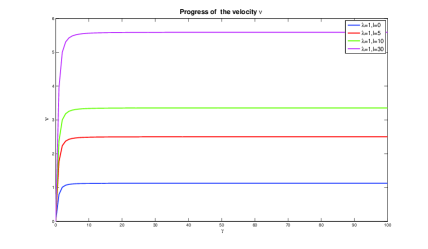
Figure 2.

5. Concluding remarks

We have constructed a set of CS obeying a Glauber-type condition for a Hamiltonian with continuous spectrum by using a tridiagonal method involving orthogonal polynomials. The basic quantities in our procedure are the parameters $\left(c_{n},d_{n}\right)$ which are related to the matrix elements $\left(a_{n},b_{n}\right)$ of the tridiagonal Hamiltonian by $\left(2.13\right)$ and $\left(2.14\right).$ More specifically, these CS are labeled by the sequence $z=c_{n}.$ But the general form $\left(2.16\right)$ is still to be exploited. Connecting these states with the Gazeau-Klauder CS was not straightforward and bridge the gap between the two approaches requires the idea of a Bayesian decomposition for the weight function in the orthogonality measure of polynomials arising from the tridiagonal method. As an example, we have the $\ell$-wave free particle for which the statistical model given by the Poisson probability distribution $\Pr\left(X=l\right)=e^{-E}E^{l}/l!,$ $l=0,1,2,...,$  $X\sim\mathcal{P}\left(E\right)$, has played a central role in writing down the convenient Bayesian decomposition for the corresponding weight function. Therefore, there should be an explanation for the appearance of the Poisson distribution having the energy $E>0$ as a parameter and the set of all angular momentum numbers $l$ as its observed data in the physics of this system.

References

- [1] E. Schrödinger, Die Naturwissenschaften, 14 (1926), 664.
- [2] R. J. Glauber, The Quantum Theory of Optical Coherence, Phys. Rev. 130 (1963), 2529-2539.
- [3] M. Schlosshauer: Decoherence and the Quantum-to-Classical Transition, The Frontiers Collection, Springer Verlag 2007.
- [4] J. R. Klauder, B. S. Skagerstam, Coherent States Applications in Physics and Mathematics. Singapore: World Scientific. 1985.
- [5] F. Grosshans, G. Van Assche, J. Wenger, R. Brouri, N. J. Cerg, Ph. Grangier: “Quantum key distribution using gaussian-modulated coherent states”, Letters to Nature, Nature 421 (2003), 238-241.
- [6] S. T. Ali, J. P. Antoine, J.P. Gazeau, Coherent States, Wavelets, and Their Generalizations. Springer, New York, 2014.
- [7] J.P. Gazeau, Coherent states in quantum physics, WILEY-VCH Verlag GMBH & Co. KGaA Weinheim 2009.
- [8] V. V. Dodonov, ”Nonclassical” states in quantum optics: a ”squeezed” review of the first 75 years. J. Opt. B Quantum Semiclass. Opt. 4(2002), R1-R33.
- [9] H. Weyl. Gruppentheorie und Quantenmechanik. (German) Reprint of the second edition. Wissenschaftliche Buchgesellschaft, Darmstadt, 1977. xi+366 pp.
- [10] A. M. Perelomov, Coherent states for arbitrary Lie group. Comm. Math. Phys. 26(1972), 222-236.
- [11] E. Onofri, A note on coherent state representations of Lie groups. J. Mathematical Phys. 16 (1975), 1087-1089.
- [12] M, Hongoh, Coherent states associated with the continuous spectrum of noncompact groups. J. Mathematical Phys. 18(1977), 2081-2084.
- [13] A. Perelomov, Generalized coherent states and their applications. Springer-Verlag, Berlin. 1986.
- [14] J. P. Gazeau and J. R. Klauder, Coherent states for systems with discrete and continuous spectrum, J. Phys. A. 32 (1999), 123.
- [15] A. Inomata, M. Sadiq, Modification of Klauder’s coherent states. 8th International Conference on Path Integrals: From Quantum Information to Cosmology, PI 2005.
- [16] J. Ben Geloun, J. Hnybida, J. R. Klauder, Coherent states for continuous spectrum operators with non-normalizable fiducial states. J. Phys. A. 45 (2012), 085301, 14 pp.
- [17] D. Popov, M. Popov, Coherent states for continuous spectrum as limiting case of hypergeometric coherent states, Romanian Reports in Physics. 68(2016), 1335-1348.
- [18] J. J. Ben Geloun, J. R. Klauder, Ladder operators and coherent states for continuous spectra. J. Phys. A. 42(2009), 375209, 9 pp.
- [19] H. A. Yamani, Z. Mouayn, Properties of shape-invariant tridiagonal Hamiltonians, Theor. Math. Phys. 203 (2020), 761.
- [20] C. P. Robert, The Bayesian Choice, Second Edition, Springer Science+Business Media, LLC, 2007.
- [21] I. S. Gradshteyn, I. M. Ryzhik. Table of integrals, series, and products. Elsevier/Academic Press, Amsterdam, seventh edition, 2007.
- [22] H. Bateman, Tables of Integral Transforms, Vol I, McGraw-Hill Book Compagny, Inc., 1954.
- [23] H. Buchholz, The Confluente Hypergeometric Function, Springer-Verlag Berlin Heidelberg GmbH 1969.