Active Contrastive Learning of
Audio-Visual Video Representations

Abstract

Contrastive learning has been shown to produce generalizable representations of audio and visual data by maximizing the lower bound on the mutual information (MI) between different views of an instance. However, obtaining a tight lower bound requires a sample size exponential in MI and thus a large set of negative samples. We can incorporate more samples by building a large queue-based dictionary, but there are theoretical limits to performance improvements even with a large number of negative samples. We hypothesize that random negative sampling leads to a highly redundant dictionary that results in suboptimal representations for downstream tasks. In this paper, we propose an active contrastive learning approach that builds an actively sampled dictionary with diverse and informative items, which improves the quality of negative samples and improves performances on tasks where there is high mutual information in the data, e.g., video classification. Our model achieves state-of-the-art performance on challenging audio and visual downstream benchmarks including UCF101, HMDB51 and ESC50.

1 Introduction

Contrastive learning of audio and visual representations has delivered impressive results on various downstream scenarios (Oord et al., 2018; Hénaff et al., 2019; Schneider et al., 2019; Chen et al., 2020). This self-supervised training process can be understood as building a dynamic dictionary per mini-batch, where “keys” are typically randomly sampled from the data. The encoders are trained to perform dictionary look-up: an encoded “query” should be similar to the value of its matching key and dissimilar to others. This training objective maximizes a lower bound of mutual information (MI) between representations and the data (Hjelm et al., 2018; Arora et al., 2019). However, such lower bounds are tight only for sample sizes exponential in the MI (McAllester & Stratos, 2020), suggesting the importance of building a large and consistent dictionary across mini-batches.

Recently, He et al. (2020) designed Momentum Contrast (MoCo) that builds a queue-based dictionary with momentum updates. It achieves a large and consistent dictionary by decoupling the dictionary size from the GPU/TPU memory capacity. However, Arora et al. (2019) showed that simply increasing the dictionary size beyond a threshold does not improve (and sometimes can even harm) the performance on downstream tasks. Furthermore, we find that MoCo can suffer when there is high redundancy in the data, because only relevant – and thus limited – parts of the dictionary are updated in each iteration, ultimately leading to a dictionary of redundant items (we show this empirically in Fig. 3). We argue that random negative sampling is much responsible for this: a randomly constructed dictionary will contain more “biased keys” (similar keys that belong to the same class) and “ineffective keys” (keys that can be easily discriminated by the current model) than a carefully constructed one. Furthermore, this issue can get aggravated when the dictionary size is large.

In this paper, we focus on learning audio-visual representations of video data by leveraging the natural correspondence between the two modalities, which serves as a useful self-supervisory signal (Owens & Efros, 2018; Owens et al., 2016; Alwassel et al., 2019). Our starting point is contrastive learning (Gutmann & Hyvärinen, 2010; Oord et al., 2018) with momentum updates (He et al., 2020). However, as we discussed above, there are both practical challenges and theoretical limits to the dictionary size. This issue is common to all natural data but is especially severe in video; successive frames contain highly redundant information, and from the information-theoretic perspective, audio-visual channels of video data contain higher MI than images because the higher dimensionality – i.e., temporal and multimodal – reduces the uncertainty between successive video clips. Therefore, a dictionary of randomly sampled video clips would contain highly redundant information, causing the contrastive learning to be ineffective. Therefore, we propose an actively sampled dictionary to sample informative and diverse set of negative instances. Our approach is inspired by active learning (Settles, 2009) that aims to identify and label only the maximally informative samples, so that one can train a high-performing classifier with minimal labeling effort. We adapt this idea to construct a non-redundant dictionary with informative negative samples.

Our approach, Cross-Modal Active Contrastive Coding (CM-ACC), learns discriminative audio-visual representations and achieves substantially better results on video data with a high amount of redundancy (and thus high MI). We show that our actively sampled dictionary contains negative samples from a wider variety of semantic categories than a randomly sampled dictionary. As a result, our approach can benefit from large dictionaries even when randomly sampled dictionaries of the same size start to have a deleterious effect on model performance. When pretrained on AudioSet (Gemmeke et al., 2017), our approach achieves new state-of-the-art classification performance on UCF101 (Soomro et al., 2012), HMDB51 (Kuehne et al., 2011), and ESC50 (Piczak, 2015b).

2 Background

Contrastive learning optimizes an objective that encourages similar samples to have similar representations than with dissimilar ones (called negative samples) (Oord et al., 2018):

$$\min_{\theta_{f},\theta_{h}}\mathbb{E}_{x\backsim p_{\mathcal{X}}}\left[-log\left(\frac{e^{f(x;\theta_{f})^{\intercal}h(x^{+};\theta_{h})}}{e^{f(x;\theta_{f})^{\intercal}h(x^{+};\theta_{h})}+e^{f(x;\theta_{f})^{\intercal}h(x^{-};\theta_{h})}}\right)\right]$$ (1)

The samples $x^{+}$ and $x^{-}$ are drawn from the same distribution as $x\in\mathcal{X}$, and are assumed to be similar and dissimilar to $x$, respectively. The objective encourages $f(\cdot)$ and $h(\cdot)$ to learn representations of $x$ such that $(x,x^{+})$ have a higher similarity than all the other pairs of $(x,x^{-})$.

We can interpret it as a dynamic dictionary look-up process: Given a “query” $x$, it finds the correct “key” $x^{+}$ among the other irrelevant keys $x^{-}$ in a dictionary. Denoting the query by $q=f(x)$, the correct key by $k^{+}=h(x^{+})$, and the dictionary of $K$ negative samples by $\{k_{i}=h(x_{i})\},i\in[1,K]$, we can express equation 1 in a softmax form, $\min_{\theta_{q},\theta_{k}}\mathbb{E}_{x\backsim p_{\mathcal{X}}}\left[-log\frac{e^{q\cdot k^{+}/\tau}}{\sum^{K}_{i=0}e^{q\cdot k_{i}/\tau}}\right]$, where $\theta_{q}$ and $\theta_{k}$ are parameters of the query and key encoders, respectively, and $\tau$ is a temperature term that controls the shape of the probability distribution computed by the softmax function.

Momentum Contrast (MoCo) decouples the dictionary size from the mini-batch size by implementing a queue-based dictionary, i.e., current mini-batch samples are enqueued while the oldest are dequeued (He et al., 2020). It then applies momentum updates to parameters of a key encoder $\theta_{k}$ with respect to parameters of a query encoder, $\theta_{k}\leftarrow m\theta_{k}+(1-m)\theta_{q}$, where $m\in[0,1)$ is a momentum coefficient. Only the parameters $\theta_{q}$ are updated by back-propagation, while the parameters $\theta_{k}$ are defined as a moving average of $\theta_{q}$ with exponential smoothing. These two modifications allow MoCo to build a large and slowly-changing (and thus consistent) dictionary.

Theoretical Limitations of Contrastive Learning. Recent work provides theoretical analysis of the shortcomings of contrastive learning. McAllester & Stratos (2020) show that lower bounds to the MI are only tight for sample size exponential in the MI, suggesting that a large amount of data are required to achieve a tighter lower bound on MI. He et al. (2020) empirically showed that increasing negative samples has shown to improve the learned presentations. However, Arora et al. (2019) showed that such a phenomenon does not always hold: Excessive negative samples can sometimes hurt performance. Also, when the number of negative samples is large, the chance of sampling redundant instances increases, limiting the effectiveness of contrastive learning. One of our main contributions is to address this issue with active sampling of negative instances, which reduces redundancy and improves diversity, leading to improved performance on various downstream tasks.

3 Approach

3.1 Cross-Modal Contrastive Representation Learning

Our learning objective encourages the representations of audio and visual clips to be similar if they come from the same temporal block of a video. Let $A=\{a_{0},\cdots,a_{N-1}\}$ and $V=\{v_{0},\cdots,v_{N-1}\}$ be collections of audio and visual clips, where each pair $(a_{i},v_{i})$ is from the same block of a video. We define query encoders $f_{a}$ and $f_{v}$ and key encoders $h_{a}$ and $h_{v}$ for audio and visual clips, respectively, with learnable parameters $\{\theta_{q}^{a},\theta_{q}^{v}\}$ for the query encoders and $\{\theta_{k}^{a},\theta_{k}^{v}\}$ for the key encoders. These encoders compute representations of audio and visual clips as queries and keys,

$$q^{v}=f_{v}(v^{query}),\>\>\>\>k^{v}=h_{v}(v^{key}),\>\>\>\>q^{a}=f_{a}(a^{query}),\>\>\>\>k^{a}=h_{a}(a^{key})$$ (2)

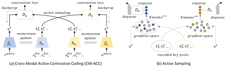
Figure 1: (a) We extend contrastive learning to the cross-modal scenario and adapt momentum contrast (MoCo) (He et al., 2020) to the dictionary update. Different from all existing work, we propose an active learning idea to the negative sampling. (b) To sample negatives, we use the gradient space of our key encoders to estimate the uncertainty of each candidate in audio/visual pools, and take a diverse set of negatives in that space using the $k$-MEANS${}^{++}_{\texttt{INIT}}$ algorithm.

We train our encoders to perform cross-modal dictionary look-up, e.g., given a query video clip $v^{query}$, we find the corresponding audio clip $a^{key}$ from a dictionary $D_{a}$. Adapting MoCo (He et al., 2020) to our cross-modal setup, we implement a queue-based dictionary $D_{a}$ that stores keys of audio clips $\{k^{a}_{i}\}_{i=1}^{K}$, where $K$ is the dictionary size. We compute the contrastive loss and backpropagate the gradients only to the visual query encoder $f_{v}$ and update the parameters $\theta_{q}^{v}$. For the audio encoder $h_{a}$, we apply the momentum update (He et al., 2020),

$$\theta_{k}^{a}\leftarrow m\theta_{k}^{a}+(1-m)\theta_{q}^{a}$$ (3)

The parameter $\theta_{q}^{a}$ is not updated in this contrastive coding step; we update it during the audio-to-visual step (similar as above with the opposite modalities). Here we explain the visual-to-audio step only; we perform bi-directional contrastive coding and train the whole model end-to-end.

3.2 Active Sampling of Negative Instances: Uncertainty and Diversity

The quality of negative samples is crucial in contrastive learning. Existing work typically adopts random negative sampling. However, we want a diverse set of negative samples so that comparisons between positive and negative pairs are the most informative they can be. Motivated by active learning (Settles, 2009), we propose a gradient-based active sampling approach to improve the quality of negative samples. In active learning, the learner chooses samples that seem maximally informative and queries an oracle for labels to obtain an optimal solution with a minimal labeling budget. Adapting this to our setting, we can empower the learner to choose the maximally informative negative samples to construct a dictionary; the main question is how to measure the informativeness of samples without labels.

One way to measure informativeness is through the lens of uncertainty: If a model is highly uncertain about its prediction of a sample, we can ensure the maximum update to the model by including the sample in a mini-batch (conversely, if the uncertainly is low for all samples in a mini-batch, the model update will be small). Ash et al. (2020) showed that gradients of a loss function with respect to the model’s most confident predictions can approximate the uncertainty of samples, demonstrating its effectiveness in active learning. They provide a theoretical justification by showing that gradient norms of the last layer of a neural network with respect to pseudo-labels provides a lower bound on gradient norms induced by any other labels. In this work, we use gradients of the last layer to measure the uncertainty and encourage our model to include samples that have the highest gradient magnitudes to constitute a dictionary.

While the uncertainty of each individual samples is important, the diversity of samples is also a critical measure of informativeness. Intuitively, it is possible that a model is highly uncertain about samples from particular semantic categories, but constructing a mini-batch of samples from just those categories can severely bias gradients and ultimately lead to a bad local minima. There are several principled approaches to ensure diversity, e.g., submodular optimization (Fujishige, 2005) and Determinantal Point Processes (DPP) (Macchi, 1975; Kulesza & Taskar, 2011). Unfortunately, those methods are typically inefficient because of the combinatorial search space (Nemhauser et al., 1978; Gilks et al., 1995). In this work, instead of using the expensive solutions, we opt to the fast solution of Ash et al. (2020) and use the initialization scheme of the $k$-MEANS$++$ seeding algorithm (Arthur & Vassilvitskii, 2007) to sample a diverse set of negative samples.

3.3 Cross-Modal Active Contrastive Coding

Algorithm 1 describes our proposed cross-modal active contrastive coding (we provide a simplified version here; we include a more detailed version and another version without active sampling in Appendix). At a high-level, we initialize the dictionaries $D_{v}$ and $D_{a}$ with $K$ randomly drawn samples from $V$ and $A$, respectively (lines 3-4). For each epoch, we construct “negative candidate pools” $U_{v}$ and $U_{a}$ with $N$ random samples from $V$ and $A$, respectively (lines 6-7). For each iteration within an epoch, we actively select the most informative negative samples $S_{v}$ and $S_{a}$ from the pools $U_{v}$ and $U_{a}$, respectively, and enqueue them into the dictionaries $D_{v}$ and $D_{a}$, respectively (lines 9-21). We then perform cross-modal contrastive coding, update the parameters of query encoders $\theta^{v}_{q}$ and $\theta^{a}_{q}$ via backpropagation, and apply momentum updates to the parameters of key encoders $\theta^{v}_{k}$ and $\theta^{a}_{k}$ (lines 22-27).

Algorithm 1 Cross-Modal Active Contrastive Coding

1:  Require: Audio-visual clips $A,V$; encoders $f_{v}$, $f_{a}$, $h_{v}$, $h_{a}$; dictionary size $K$; pool size $N$; batch size $M$

2:  Initialize parameters, $\theta_{q}^{v},\theta_{k}^{v},\theta_{q}^{a},\theta_{k}^{a}\backsim Uniform(0,1)$

3:  Draw random dictionary, $D_{v}\leftarrow\{v_{1},\cdots,v_{K}\}\backsim V$, $D_{a}\leftarrow\{a_{1},\cdots,a_{K}\}\backsim A$

4:  Encode dictionary samples, $k^{v}_{i}\leftarrow h_{v}(v_{i}),\forall v_{i}\in D_{v}$, $k^{a}_{i}\leftarrow h_{a}(a_{i}),\forall a_{i}\in D_{a}$

5:  for $epoch=1$ to #epochs: do

6:     Draw random pool, $U_{v}\leftarrow\{v_{1},\cdots,v_{N}\}\backsim V$, $U_{a}\leftarrow\{a_{1},\cdots,a_{N}\}\backsim A$

7:     Encode pool samples, $k^{v}_{n}\leftarrow h_{v}(v_{n}),\forall v_{n}\in U_{v}$, $k^{a}_{n}\leftarrow h_{a}(a_{n}),\forall a_{n}\in U_{a}$

8:     for $t=1$ to #mini-batches: do

9:        Draw mini-batch, $B_{v}\leftarrow\{v_{1},\cdots,v_{M}\}\backsim V$, $B_{a}\leftarrow\{a_{1},\cdots,a_{M}\}\backsim A$

10:        $\triangleright$ Active sampling of negative video keys for $D_{v}$

11:        Encode mini-batch samples, $q^{a}_{i}\leftarrow f_{a}(a_{i}),\forall a_{i}\in B_{a}$

12:        Compute pseudo-labels, $\tilde{y}^{v}_{n}\leftarrow\arg\max p({\hat{y}^{v}_{n}}|v_{n},B_{a})$, $\forall v_{n}\in U_{v}$\$D_{v}$

13:        Compute gradients $g_{v_{n}}$ using the pseudo-labels $\tilde{y}^{v}_{n}$, $\forall n\in[1,N]$

14:        Obtain $S_{v}\leftarrow k\mbox{-{MEANS}}^{++}_{\texttt{INIT}}\left(\{g_{v_{n}}:v_{n}\in U_{v}\backslash D_{v}\},\#\mbox{seeds}=M\right)$

15:        Update $D_{v}\leftarrow\mbox{{ENQUEUE}}(\mbox{{DEQUEUE}}(D_{v}),S_{v})$

16:        $\triangleright$ Active sampling of negative audio keys for $D_{a}$

17:        Encode mini-batch samples, $q^{v}_{i}\leftarrow f_{v}(v_{i}),\forall v_{i}\in B_{v}$

18:        Compute pseudo-label, $\tilde{y}^{a}_{n}\leftarrow\arg\max p({\hat{y}^{a}_{n}}|a_{n},B_{v})$, $\forall a_{n}\in U_{a}$\$D_{a}$

19:        Compute gradients $g_{a_{n}}$ using the pseudo-labels $\tilde{y}^{a}_{n}$, $\forall n\in[1,N]$

20:        Obtain $S_{a}\leftarrow k\mbox{-{MEANS}}^{++}_{\texttt{INIT}}\left(\{g_{a_{n}}:a_{n}\in U_{a}\backslash D_{a}\},\#\mbox{seeds}=M\right)$

21:        Update $D_{a}\leftarrow\mbox{{ENQUEUE}}(\mbox{{DEQUEUE}}(D_{a}),S_{a})$

22:        $\triangleright$ Cross-modal contrastive predictive coding

23:        Encode mini-batch samples, $k^{v}_{i}\leftarrow h_{v}(v_{i}),\forall v_{i}\in B_{v}$, $k^{a}_{i}\leftarrow h_{a}(a_{i}),\forall a_{i}\in B_{a}$

24:        Compute $p(y^{v}_{i}|v_{i},a_{i},D_{a})$ and $p(y^{a}_{i}|a_{i},v_{i},D_{v})$, $\forall i\in[1,M]$

25:        $\triangleright$ Update model parameters

26:        Update parameters of query encoders $\theta_{q}^{v}$ and $\theta_{q}^{a}$ with backpropagation

27:        Momentum update parameters of key encoders $\theta_{k}^{v}$ and $\theta_{k}^{a}$

28:     end for

29:  end for

30:  return  Optimal solution $\theta_{q}^{v},\theta_{k}^{v},\theta_{q}^{a},\theta_{k}^{a}$

Active sampling. To measure uncertainty, we define a pseudo-label space induced by the queries from the other modality, and take the gradient of the last layer of a query encoder with respect to the most confident prediction, which we call the pseudo-label $\tilde{y}$. For instance, in the case of sampling negative video keys from the pool $U_{v}$ (lines 10-15), we compute the pseudo-posterior of a video key $v_{n}\in U_{v}\backslash D_{a}$,

$$p({\hat{y}^{v}_{n}}|v_{n},B_{a})=\frac{\exp(k_{n}^{v}\cdot q_{j}^{a})}{\sum_{i=1}^{M}\exp(k_{n}^{v}\cdot q_{i}^{a})},\forall j\in[1,M]$$ (4)

where $B_{a}$ is the current mini-batch of audio queries and defines the pseudo-label space. Note that we consider only the samples in $U_{v}\backslash D_{v}$ to rule out samples already in $D_{v}$. Intuitively, this computes the posterior by the dot-product similarity between $v_{n}$ and all $q^{a}_{i}\in B_{a}$, producing an $M$-dimensional probability distribution. We then take the most confident class category as the pseudo-label $\tilde{y}^{v}_{n}$ (line 12) and compute the gradient according to the cross-entropy loss

$$g_{v_{n}}=\frac{\partial}{\partial\theta_{last}}\mathcal{L}_{CE}\left(p(\hat{y}^{v}_{n}|v_{n},B_{a}),\tilde{y}^{v}_{n}\right)|_{\theta=\theta_{q}^{a}}$$ (5)

where $\theta_{last}$ is the parameters of the last layer of $\theta$ (in this case, $\theta^{a}_{q}$ of the audio query encoder $h_{a}$). Intuitively, the gradient $g_{v_{n}}$ measures the amount of change – and thus, the uncertainty – $v_{n}$ will bring to the audio query encoder $h_{a}$.

One can interpret this as a form of online hard negative mining: The gradient is measured with respect to the most probable pseudo-label $\tilde{y}_{n}^{v}$ induced by the corresponding audio query $q_{j}^{a}$. When we compute the contrastive loss, the same audio query will be maximally confused by $v_{n}$ with its positive key $v^{+}$ per dot-product similarity, and $v_{n}$ in this case can serve as a hard negative sample.

Next, we obtain the most diverse and highly uncertain subset $S_{v}\subseteq U_{v}\backslash D_{v}$ using the initialization scheme of $k\mbox{-{MEANS}}^{++}$ (Arthur & Vassilvitskii, 2007) over the gradient embeddings $g_{v}$ (line 14). The $k\mbox{-{MEANS}}^{++}$ initialization scheme finds the seed cluster centroids by iteratively sampling points with a probability in proportion to their squared distances from the nearest centroid that has already been chosen (we provide the exact algorithm in the Appendix). Intuitively, this returns a diverse set of instances sampled in a greedy manner, each of which has a high degree of uncertainty measured as its squared distances from other instances that have already been chosen. Finally, we enqueue $S_{v}$ into $D_{v}$ and dequeue the oldest batch from $D_{v}$ (line 15). We repeat this process to sample negative audio keys (lines 16-21); this concludes the active sampling process for $D_{v}$ and $D_{a}$.

Cross-modal contrastive coding. Given the updated $D_{v}$ and $D_{a}$, we perform cross-modal contrastive coding. For visual-to-audio coding, we compute the posteriors of all video samples $v_{i}\in B_{v}$ with respect to the negative samples in the audio dictionary $D_{a}$,

$$p(y^{v}_{i}|v_{i},a_{i},D_{a})=\frac{\exp(q^{v}_{i}\cdot k^{a}_{i}/\tau)}{\sum_{j=0}^{K}\exp(q^{v}_{i}\cdot k^{a}_{j}/\tau)},\forall i\in[1,M]$$ (6)

where the posterior is defined over a cross-modal space with one positive and $K$ negative pairs (line 24). Next, we backpropagate gradients only to the query encoders $f_{v}$ and $f_{a}$ (line 26),

$$\theta_{q}^{v}\leftarrow\theta_{q}^{v}-\gamma\nabla_{\theta}\mathcal{L}_{CE}(p(y^{v}|\>\cdot\>),y^{v}_{gt})|_{\theta=\theta_{q}^{v}},\>\>\theta_{q}^{a}\leftarrow\theta_{q}^{a}-\gamma\nabla_{\theta}\mathcal{L}_{CE}(p(y^{a}|\>\cdot\>),y^{a}_{gt})|_{\theta=\theta_{q}^{a}}$$ (7)

while applying momentum update to the parameters of the key encoders $h_{v}$ and $h_{a}$ (line 27),

$$\theta_{k}^{v}\leftarrow m\theta_{k}^{v}+(1-m)\theta_{q}^{v},\>\>\theta_{k}^{a}\leftarrow m\theta_{k}^{a}+(1-m)\theta_{q}^{a}$$ (8)

The momentum update allows the dictionaries to change their states slowly, thus making them consistent across iterations. However, our cross-modal formulation can cause inconsistency in dictionary states because the gradient used to update query encoders are not directly used to update the corresponding key encoders. To improve stability, we let the gradients flow in a cross-modal fashion, updating part of $f_{v}$ and $h_{a}$ using the same gradient signal from the contrastive loss. We do this by adding one FC layer on top of all encoders and applying momentum update to their parameters. For example, we apply momentum update to the parameters of the FC layer on top of $h_{a}$ using the parameters of the FC layer from $f_{v}$. We omit this in Alg. 1 for clarity but show its importance in our ablation experiments (XMoCo (w/o fcl) in Table 1).

4 Related Work

Self-supervised learning has been studied in vision, language, and audio domains. In the image domain, one popular idea is learning representations by maximizing the MI between different views of the same image (Belghazi et al., 2018; Hjelm et al., 2018; Tian et al., 2019; He et al., 2020). In the video domain, several approaches have exploited the spatio-temporal structure of video data to design efficient pretext tasks, e.g. by adopting ordering (Sermanet et al., 2017; Wang et al., 2019b), temporal consistency (Dwibedi et al., 2019), and spatio-temporal statistics (Xu et al., 2019; Wang et al., 2019a; Han et al., 2019). In the language domain, the transformer-based approaches trained with the masked language model (MLM) objective has been the most successful (Devlin et al., 2019; Liu et al., 2019; Yang et al., 2019). Riding on the success of BERT (Devlin et al., 2019), several concurrent approaches generalize it to learn visual-linguistic representations (Lu et al., 2019; Li et al., 2020; Su et al., 2019; Tan & Bansal, 2019; Li et al., 2019). CBT (Sun et al., 2019a) and VideoBERT (Sun et al., 2019b) made efforts on adapting BERT-style pretraining for video.

Besides vision and language signals, several approaches learn audio-visual representations in a self-supervised manner (Owens et al., 2016; Arandjelovic & Zisserman, 2017; Owens & Efros, 2018; Owens et al., 2016). Recently, audio-visual learning has been applied to enable interesting applications beyond recognition tasks, such as sound source localization/separation (Zhao et al., 2018; Arandjelovic & Zisserman, 2018; Gao et al., 2018; Gao & Grauman, 2019a; b; Ephrat et al., 2018; Gan et al., 2020; Zhao et al., 2019; Yang et al., 2020) and visual-to-sound generation (Hao et al., 2018; Zhou et al., 2018). The work of Owens & Efros (2018), Korbar et al. (2018), and Alwassel et al. (2019) are similar in spirit to our own, but our technical approach differs substantially in the use of active sampling and contrastive learning.

Hard negative mining is used in a variety of tasks, such as detection (Li et al., 2020), tracking (Nam & Han, 2016), and retrieval (Faghri et al., 2017; Pang et al., 2019), to improve the quality of prediction models by incorporating negative examples that are more difficult than randomly chosen ones. Several recent work have focused on finding informative negative samples for contrastive learning. Wu et al. (2020) show that the choice of negative samples is critical in contrastive learning and propose variational extension to InfoNCE with modified strategies for negative sampling. Iscen et al. (2018) propose hard examples mining for effective finetuning of pretrained networks. Cao et al. (2020) utilize negative sampling to reduce the computational cost. In the context of audio-visual self-supervised learning, Korbar et al. (2018) sample negatives under the assumption that the smaller the time gap is between audio and visual clips of the same video, the harder it is to differentiate them (and thus they are considered hard negatives). Our proposed approach does not make such an assumption and estimates the hardness of negatives by directly analyzing the magnitude of the gradients with respect to the contrastive learning objective.

$\#$	Approach	Pretrain Obj.	UCF101	HMDB51	ESC50	Gains
①	Scratch	-	63.3	29.7	54.3
②	Supervised	Supervised	86.9	53.1	78.3
③	SMoCo	Uni. rand.	70.7	35.2	69.0
④	XMoCo (w/o fcl)	Cross rand.	72.9 ($\uparrow$2.2)	37.5 ($\uparrow$2.3)	70.9 ($\uparrow$1.9)	$\Delta(④-③)$
⑤	XMoCo	Cross rand.	74.1 ($\uparrow$1.2)	38.7 ($\uparrow$1.2)	73.0 ($\uparrow$2.1)	$\Delta(⑤-④)$
⑥	CM-ACC (w/o fcl)	Cross active	75.8 ($\downarrow$1.4)	39.1 ($\downarrow$1.5)	77.3 ($\downarrow$1.9)	$\Delta(⑥-⑦)$
⑦	CM-ACC	Cross active	77.2 ($\uparrow$3.1)	40.6 ($\uparrow$1.9)	79.2 ($\uparrow$6.2)	$\Delta(⑦-⑤)$

Table 1: Top-1 accuracy of unimodal vs. cross-modal pretraining on downstream tasks.

5 Experiments

Experimental Setting. We use 3D-ResNet18 (Hara et al., 2018) as our visual encoders ($f_{v}$ and $h_{v}$) in most of the experiments. We also use R(2+1)D-18 (Tran et al., 2018) to enable a fair comparison with previous work (see Table 4). For audio encoders ($f_{a}$ and $h_{a}$), we adapt ResNet-18 (He et al., 2016) to audio signals by replacing 2D convolution kernels with 1D kernels. We employ Batch Normalization (BN) (Ioffe & Szegedy, 2015) with the shuffling BN (He et al., 2020) in all our encoders. All models are trained end-to-end with the ADAM optimizer (Kingma & Ba, 2014) with an initial learning rate $\gamma=10^{-3}$ after a warm-up period of 500 iterations. We use the mini-batch size $M=128$, dictionary size $K=30\times 128$, pool size $N=300\times 128$, momentum $m=0.999$, and temperature $\tau=0.7$. We used 40 NVIDIA Tesla P100 GPUs for our experiments.

We pretrain our model on Kinetics-700 (Carreira et al., 2019) and AudioSet (Gemmeke et al., 2017) when comparing with state-of-the-art approaches. For Kinetics-700, we use 240K randomly selected videos that contain the audio channel. On AudioSet, we use both a subset of 240K randomly selected videos and the 1.8M full set. For our ablation study, we use Kinetics-Sound (Arandjelovic & Zisserman, 2017) that contains 22K videos from 34 classes that are potentially manifested both visually and audibly, and thus provides a relatively clean testbed for ablation purposes. As for downstream tasks, we evaluate our models on action recognition using UCF101 (Soomro et al., 2012) and HMDB51 (Kuehne et al., 2011), and on sound classification using ESC50 (Piczak, 2015b).

Unimodal vs. cross-modal pretraining. To validate the benefits of cross-modal pretraining, we compare it to its unimodal counterparts. We pretrain our model on Kinetics-Sound with a randomly sampled dictionary (similar to MoCo (He et al., 2020)); we call this XMoCo. For the unimodal case, we pretrain two models on visual clips and audio clips, respectively; we call these SMoCo. We also compare ours with a model trained from scratch (Scratch), and a model pretrained on Kinetics-Sound in a fully-supervised manner (Supervised). Lastly, we include XMoCo (w/o fcl) that is identical to XMoCo except that we do not include the additional FC layers on top of the encoders. All these models are finetuned end-to-end on each downstream task using the same protocol.

Table 1 shows the top-1 accuracy of each downstream task. We observe that all the self-supervised models outperform Scratch on all downstream tasks, suggesting the effectiveness of pretraining with contrastive learning. We also see that our cross-modal objective outperforms the unimodal objective ($\Delta$(④-③)). The comparisons between XMoCo vs. XMoCo (w/o fcl) and CM-ACC vs. CM-ACC (w/o fcl) show the effectiveness of the additional FC layer on top of the encoders ($\Delta$(⑤-④), $\Delta$(⑥-⑦)). When adding the FC layer, the performance further improves on all three benchmarks. This shows the importance of letting the gradients flow in a cross-modal fashion. Finally, the performance gap with the full-supervised case shows there is still room for improvement in the self-supervised approaches.

Next, we compare the number of unique categories the sampled instances originally belong to, using the ground-truth labels provided in the dataset. Our logic is that the more categories the samples come from, the more diverse and less redundant the samples are. We train these on UCF-101 over 300 iterations with different mini-batch sizes, $M\in\{32,64,128\}$. Fig. 2 shows that active sampling selects more categories than random sampling across all three mini-batch sizes. At $M=128$, active sampling (with gradient embedding) covers 60-70$\%$ of categories on UCF101, which is substantially more diverse than random sampling (30-40$\%$). (A plot showing the probability of sampling unique negatives (instances from different categories) is shown in Appendix Figure 4.) While both sampling schemes perform similarly in early iterations, active sampling starts choosing more diverse instances as the training progresses; this is because the gradient embedding becomes more discriminative with respect to the uncertainty.

Random vs. active sampling.

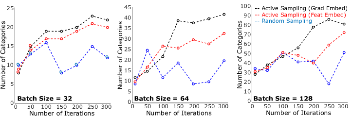
Figure 2: Effects of random sampling and active sampling on the number of categories.

To validate the benefit of active sampling over random sampling, we compare models pretrained with different sampling approaches on downstream tasks. As shown in Table 1, our CM-ACC outperforms the XMoCo, which uses random sampling, by large margins, i.e. 3.1$\%$, 1.9$\%$, and 6.2$\%$ on UCF101, HMDB51, and ESC50, respectively ($\Delta$(⑦-⑤)).

Pretrain Objective	Embedding Space	UCF101	HMDB51	ESC50
Cross-modal active	Feature Embedding	74.5	38.2	75.1
Cross-modal active	Gradient Embedding	77.2 ($\uparrow$2.7)	40.6 ($\uparrow$2.4)	79.2 ($\uparrow$4.1)

Table 2: Top-1 accuracy on downstream tasks: feature- vs. gradient-based embedding.

	UCF101			HMDB51
	$M$=32	$M$=64	$M$=128	$M$=32	$M$=64	$M$=128
Random	61.9	63.1	66.9	33.1	33.8	35.8
OHEM	50.2 (-11.7)	60.8 (-2.3)	65.7 (-1.2)	26.8 (-6.3)	30.1 (-3.7)	33.2 (-2.6)
Active	78.0 (+16.1)	78.9 (+15.8)	79.2 (+12.3)	41.2 (+8.1)	42.3 (+8.5)	42.6 (+6.8)

Table 3: Online hard example mining (OHEM) (Shrivastava et al., 2016) vs. our active sampling

Feature vs. gradient embedding. We compare two ways to do active sampling: using gradient embeddings (Eqn. 5) and feature embeddings (the outputs from $h_{a}$ and $h_{v}$) when selecting the seed centroids with $k\mbox{-{MEANS}}^{++}$. Fig. 2 shows that gradient embeddings produce a more diverse set of negative samples than feature embeddings; this is consistent across all three batch sizes. Table 2 shows that this diversity helps achieve better downstream performances across all three benchmarks. Fig. 5 (in Appendix) provides further insights, showing that the samples with high gradient magnitudes tend to be more informative negative samples.

From a theoretical aspect, the gradient norm induced by each candidate with computed pseudo labels estimates the candidates influence on the current model. The gradient embeddings convey information both about the model’s uncertainty and potential update direction upon receiving a candidate. However, such messages are missing from the feature embeddings. This shows the importance of considering both uncertainty and diversity when selecting random samples: the $k\mbox{-{MEANS}}^{++}$ ensures the diversity in the sample set, but without the uncertainty measure we lose important discriminative information from the candidates.

Method	Architecture	Pretrained on (size)	UCF101	HMDB51
Scratch	3D-ResNet18	-	46.5	17.1
Supervised (Patrick et al., 2020)	R(2+1)D-18	Kinetics400 (N/A)	95.0	70.4
ShufflAL (Misra et al., 2016)	CaffeNet	UCF/HMDB	50.2	18.1
DRL (Buchler et al., 2018)	CaffeNet	UCF/HMDB	58.6	25.0
OPN (Lee et al., 2017)	VGG	UCF/HMDB	59.8	23.8
DPC (Han et al., 2019)	3D-ResNet18	UCF101	60.6	-
MotionPred (Wang et al., 2019a)	C3D	Kinetics400 (N/A)	61.2	33.4
RotNet3D (Jing & Tian, 2018)	3D-ResNet18	Kinetics400 (N/A)	62.9	33.7
ST-Puzzle (Kim et al., 2019)	3D-ResNet18	Kinetics400 (N/A)	65.8	33.7
ClipOrder (Xu et al., 2019)	R(2+1)D-18	Kinetics400 (N/A)	72.4	30.9
CBT (Sun et al., 2019a)	S3D $\&$ BERT	Kinetics600 (500K)	79.5	44.6
DPC (Han et al., 2019)	3D-ResNet34	Kinetics400 (306K)	75.7	35.7
SeLaVi (Asano et al., 2020)	R(2+1)D-18	Kinetics400 (240K)	83.1	47.1
AVTS (Korbar et al., 2018)	MC3	Kinetics400 (240K)	85.8	56.9
XDC (Alwassel et al., 2019)	R(2+1)D-18	Kinetics400 (240K)	84.2	47.1
AVID (Morgado et al., 2020)	R(2+1)D-18	Kinetics400 (240K)	87.5	60.8
GDT (Patrick et al., 2020)	R(2+1)D-18	Kinetics400 (N/A)	89.3	60.0
AVTS (Korbar et al., 2018)	MC3	AudioSet (240K)	86.4	–
AVTS (Korbar et al., 2018)	MC3	AudioSet (1.8M)	89.0	61.6
XDC (Alwassel et al., 2019)	R(2+1)D-18	AudioSet (1.8M)	91.2	61.0
AVID (Morgado et al., 2020)	R(2+1)D-18	AudioSet (1.8M)	91.5	64.7
GDT (Patrick et al., 2020)	R(2+1)D-18	AudioSet (1.8M)	92.5	66.1
Ours	3D-ResNet18	UCF101	69.1 (+8.5)	33.3 (+8.3)
	3D-ResNet18	Kine.-Sound (14K)	77.2 (+16.6)	40.6 (+15.6)
	3D-ResNet18	Kinetics700 (240K)	90.2 (+0.9)	61.8 (+1.0)
	3D-ResNet18	AudioSet (240K)	90.7 (+1.4)	62.3 (+1.5)
	3D-ResNet18	AudioSet (1.8M)	94.1 (+1.6)	66.8 (+0.7)
	R(2+1)D-18	AudioSet (1.8M)	93.5 (+1.0)	67.2 (+1.1)

Table 4: Comparison of SOTA approaches on action recognition. We specify pretraining dataset and the number of samples used if they are reported in the original papers (N/A: not available).

Online hard example mining vs. active sampling. We compare our approach to online hard example mining (OHEM) (Shrivastava et al., 2016), which constructs negative samples by explicitly choosing the ones that incur high loss values. Specifically, we compute the pseudo-labels for all keys (negative sample candidates) with a given mini-batch of queries. We then compute the classification loss based on these pseudo labels and select the top $M$ keys with the highest loss values. We pretrain the models on Kinetics-700 (Kay et al., 2017) and report the top-1 accuracy on UCF101 (Soomro et al., 2012) and HMDB51 (Kuehne et al., 2011). We use the same architecture and hyper-parameters; the only difference is the sampling approach.

Table 3 shows OHEM is generally less effective than both random sampling and our active sampling. Intuitively, OHEM promotes the dictionary to contain the most challenging keys for a given mini-batch of queries. Unfortunately, this causes OHEM to produce a redundant and biased dictionary, e.g., negative samples coming from a particular semantic category. Our results show that, when $M$ (mini-batch size) is small, the performance of OHEM is even worse than random sampling, although the gap between OHEM and random sampling decreases as $M$ increases. We believe this is because OHEM has a higher chance of selecting similar negative instances. When $M$ is large, this issue can be mitigated to some extent, but the performance still falls behind ours by a large margin. This suggests the importance of having a diverse set of negative samples, which is unique in our approach.

Method	Architecture	Pretrained on (size)	ESC50
Random Forest (Piczak, 2015b)	MLP	ESC50	44.3
Piczak ConvNet (Piczak, 2015a)	ConvNet-4	ESC50	64.5
ConvRBM (Sailor et al., 2017)	ConvNet-4	ESC50	86.5
SoundNet (Aytar et al., 2016)	ConvNet-8	SoundNet (2M+)	74.2
$L^{3}$-Net (Arandjelovic & Zisserman, 2017)	ConvNet-8	SoundNet (500K)	79.3
AVTS (Korbar et al., 2018)	VGG-8	Kinetics (240K)	76.7
XDC (Alwassel et al., 2019)	ResNet-18	Kinetics (240K)	78.0
AVID (Morgado et al., 2020)	ConvNet-9	Kinetics (240K)	79.1
AVTS (Korbar et al., 2018)	VGG-8	AudioSet (1.8M)	80.6
XDC (Alwassel et al., 2019)	ResNet-18	AudioSet (1.8M)	84.8
AVID (Morgado et al., 2020)	ConvNet-9	AudioSet (1.8M)	89.2
GDT (Patrick et al., 2020)	ResNet-9	AudioSet (1.8M)	88.5
Ours	ResNet-18	Kinetics700 (240K)	80.2 (+1.1)
		AudioSet (240K)	80.9 (+1.8)
		AudioSet (1.8M)	90.8 (+1.6)

Table 5: Comparision of SOTA approaches on audio event classification.

Comparisons with SOTA. Table 4 shows our approach outperforms various self-supervised approaches on action recognition. For fair comparisons, we group the SOTA approaches by different pretraining dataset sizes, i.e. small-scale (UCF/HMDB), medium-scale (Kinetics), and large-scale (AudioSet). Our gains are calculated according to this grouping. As we can see, our approach outperforms SOTA approaches across all groups. Compared with GDT (Patrick et al., 2020), the current top performing model on cross-modal self-supervised learning, our model outperforms it by 1.6 $\%$ on UCF101 and 1.1 $\%$ on HMDB51. Table 5 shows audio classification transfer results. For Kinetics and AudioSet (240K), our model outperforms the current state-of-the-art, AVID (79.1$\%$) by 0.1$\%$ and 1.8$\%$ on Kinetics and AudioSet 240K, respectively. Our approach also outperforms AVID (89.2$\%$) pretrained on AudioSet (1.8M) by 1.6$\%$.

6 Conclusion

We have shown that random sampling could be detrimental to contrastive learning due to the redundancy in negative samples, especially when the sample size is large, and have proposed an active sampling approach that yields diverse and informative negative samples. We demonstrated this on learning audio-visual representations from unlabeled videos. When pretrained on AudioSet, our approach outperforms previous state-of-the-art self-supervised approaches on various audio and visual downstream benchmarks. We also show that our active sampling approach significantly improves the performance of contrastive learning over random and online hard negative sampling approaches.

Appendix A Details on Data Processing

We preprocess video frames by sampling at 10 FPS and applying random cropping, horizontal flipping, gray-scaling, and temporal jittering. We resize video frames to 3-channel images of $224\times 224$; we set the clip length to 16 frames during pretraining, and 32 frames during finetuning on downstream tasks. For audio channel, we extract mel-spectrograms from the raw waveform using the LibROSA library and get a $80\times T$ matrix with 80 frequency bands; T is proportionate to the length of an audio clip. We then segment the mel-spectrogram according to the corresponding video clips to ensure temporal synchrony. We treat the mel-spectrograms as an 80-channel 1D signal.

As for downstream tasks, we evaluate our models on action recognition using UCF101 (Soomro et al., 2012) and HMDB51 (Kuehne et al., 2011), and on sound classification using ESC50 (Piczak, 2015b). UCF101 contains 13K video clips from 101 action categories, HMDB51 contains 7K video clips from 51 categories, and ESC50 has 2K audio clips from 50 categories. UCF101 and HMDB51 have 3 official train/test splits, while ESC50 has 5 splits. We conduct our ablation study using split-1 of each dataset. We report our average performance over all splits when we compare with prior work.

Appendix B Additional Experiments

Effect of mutual information. We investigate the impact of the amount of MI on contrastive learning using the Spatial-MultiOmniglot dataset (Ozair et al., 2019). It contains paired images $(x,y)$ of Omniglot characters (Lake et al., 2015) with each image arranged in an $m\times n$ grid (each grid cell is $32\times 32$ pixels). Let $l_{i}$ be the alphabet size for the $i^{th}$ character in each image, then the MI $I(x,y)=\sum_{i=1}^{mn}logl_{i}$. This way, we can easily control the MI by adding or removing characters. We follow the experimental protocol of Ozair et al. (Ozair et al., 2019), keeping the training dataset size fixed at 50K and using the same alphabet sets: Tifinagh (55 characters), Hiragana (52), Gujarati (48), Katakana (47), Bengali (46), Grantha (43), Sanskrit (42), Armenian (41), and Mkhedruli (41).

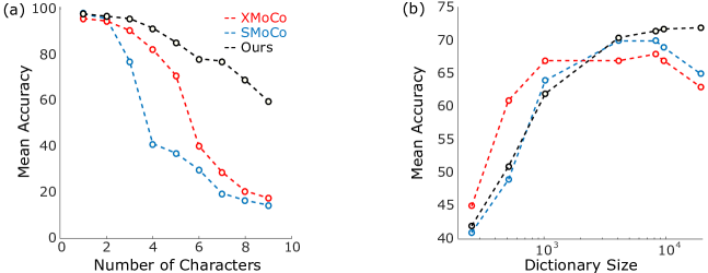
Figure 3: The effect of a) mutual information (Spatial-MultiOmniglot) and b) dictionary size on the accuracy of classification (UCF101).

Fig. 3(a) shows the results as the number of characters (and thus the MI) increases. We see that all approaches achieve nearly 99$\%$ accuracy with less than 3 characters; this is the case when the exponent of the MI is smaller than the dataset size (50K), i.e., $e^{I(x,y)}=55$ with one character, $e^{I(x,y)}=2,860$ with 2 characters. However, starting from 3 characters, the performance of the regular MoCo (SMoCo) drops significantly; this is because the exponent of the MI (=137,280 (55$\times$52$\times$48)) is much larger than the dataset size. Although our model also drops performance when the MI is increased, it outperforms the other approaches by a large margin. We also observe that XMoCo outperforms SMoCo in mild conditions (1-5 characters) but performs nearly the same as SMoCo with severe conditions (6-9 characters). This suggests that, while cross-modal prediction helps to learn good representations, it also suffers with the same issue when the MI is large, thus adopting active sampling is beneficial.

Effect of dictionary size. Fig. 3 (b) shows how the dictionary size affects downstream task performance. Here we pretrain our model on Kinetics-700 and finetune it on UCF-101. Overall, all three approaches benefit from large dictionaries up to a threshold (at about $10^{3}$), which is consistent with previous empirical findings (He et al., 2020). However, both XMoCo and SMoCo starts deteriorating performance after about $10^{4}$ (which is consistent with previous theoretical claims of Arora et. al (Arora et al., 2019)), whereas ours do not suffer even after $10^{4}$. This suggests that there are performance limits by simply increasing the size of a randomly-sampled dictionary, and also shows the benefit of our active sampling approach.

Effect of pretraining dataset sizes. We investigate the effects of the size of pretraining datasets, using Kinetics-Sound (22k), Kinetics (240K), and AudioSet (1.8M). We vary pretraining conditions while using the same protocol to finetune the models end-to-end on downstream tasks.

Table 6 shows that our model benefits from pretraining on video data, and that the performance improves as we use a large pretraining video dataset (Kinetics and AudioSet) than the relatively smaller dataset (Kinetics-Sound). Notably, our approach even outperforms the fully-supervised pretraining approaches by pretraining on a larger video dataset (1.0$\%$, 3.6$\%$, and 8.5$\%$ improvement on UCF101, HMDB51, and ESC50, respectively.)

Approach	Dataset	UCF101	HMDB51	ESC50
Supervised	ImageNet (1.2M)	82.8†	46.7†	–
	Kinetics-Sound (22K)	86.9∗	53.1∗	$78.3^{*}$
	Kinetics400 (240K)	93.1†	63.6†	$82.3^{*}$
CM-ACC	Kinetics-Sound (22K)	77.2	40.6	77.3
	Kinetics700 (240K)	90.2 (-2.9)	61.8 (-1.8)	79.2 (-3.1)
	AudioSet (1.8M)	94.1 (+1.0)	67.2 (+3.6)	90.8 (+8.5)

Table 6: Top-1 accuracy of CM-ACC pretrained on different datasets vs. fully-supervised counterparts (Supervised). ^†: the results are excerpted from Patrick et al. (2020), ^∗: our results.

Diversity of random vs. active sampling. To compare the diversity of the chosen negatives by random vs. active sampling, we plot the probability of them on sampling of unique negatives (instances from different categories). The more categories the samples come from, we get more diverse and less redundant samples. We train these on UCF-101 over 300 iterations with different mini-batch sizes, $M\in\{32,64,128\}$. As shown in Figure 4, the active sampling selects more categories than random sampling across all three mini-batch sizes. At $M=128$, active sampling (with gradient embedding) covers 60-70% of categories on UCF101, which is substantially more diverse than random sampling (30-40%).

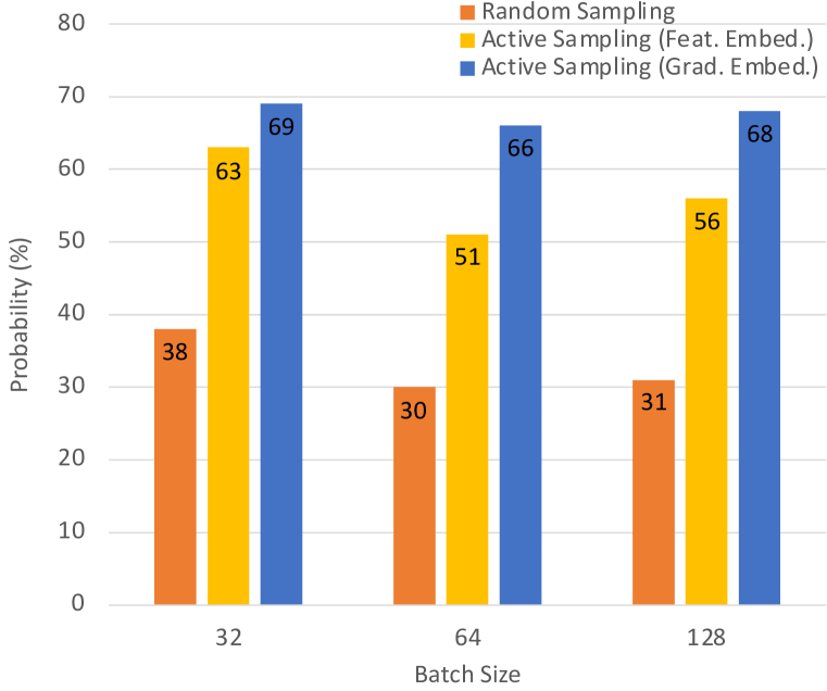
Figure 4: Probability of sampling unique negatives (instances from different categories) in the random vs. active sampling conditions. We compute the probabilities by averaging the number of unique categories across iterations and dividing them by their batch size.

Appendix C Visualization of negative instances

Figure 5 shows negative instances selected by active sampling and random sampling when we use audio clips as the query. We visualize the center frames of the selected video clips. We can see that our approach selects more challenging examples than the random sampling approach. For instance, given a query opening bottle, our approach selected video clips from the same or similar semantic categories, e.g. drinking shot and opening bottle. Given snowboarding, our approach selected more video clips related to categories containing the snow scene, e.g. ice fishing, snow kiting, and tobogganing.

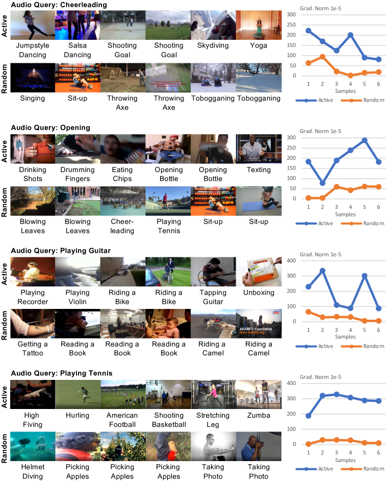
Figure 5: Center frames of video clips and their gradient norms selected by active sampling and random sampling.

Furthermore, we also find that our approach selects more diverse negative samples. For example, given a query snowboarding, active sampling selected video clips from 4 different categories related to the snow scene: (ice fishing, playing ice hockey, snow kiting, and tobogganing). In comparison, the random sampling approach yields fewer semantic categories in general. This suggests that our active sampling approach produces more ‘challenging’ and ‘diverse’ negative instances than the random sampling approach.

To clearly investigate the relationship between negative samples and their gradient magnitudes, we show the gradient norm of each visualized sample in Figure 5. We can see that hard negatives tend to have larger gradient norms than easy negatives. Given a query Playing guitar, video clips containing the concept of “playing instruments” yield the higher gradient norms, i.e. playing violin (333.87) and tapping guitar (301.35), while concepts that are easy to discriminate, e.g., riding a camel yield a significantly smaller gradient norm (5.92). This provides evidence showing the gradient magnitude is effective in measuring the uncertainty of the current model, i.e., highly-uncertain samples (hard negatives) tend to yield gradients with larger magnitudes, while highly-confident samples (easy negatives) tend to have smaller gradient magnitudes.

Appendix D When would cross-modal contrastive learning fail?

In general, cross-modal video representation learning is based on an assumption that the natural correspondence between audio and visual channels could serve as a useful source of supervision. While intuitive, this assumption may not hold for certain videos in-the-wild, which may cause the model to learn suboptimal representations. To investigate when our approach succeeds and fails, we conduct a post-hoc analysis by using thehttps://www.overleaf.com/project/5ded2abe1c17bc00011e5da8 ground-truth semantic category labels provided in Kinetics-700 (Carreira et al., 2019) (which is not used during pretraining). Specifically, we use our pretrained model to solve the audio-visual contrastive pretext task (Eqn.(7) in the main paper) and keep track of the prediction results (correct/incorrect). We then average the pretext task accuracy over 100 randomly chosen samples for each action category.

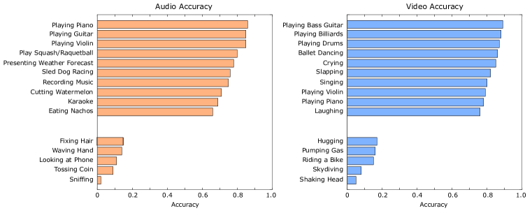
Figure 6: Distribution of Kinetics-700 (Carreira et al., 2019) categories sorted by the prediction accuracy.

Figure 6 shows the top-10 and bottom-5 classes by using both audio (left) and video (right) as the query. We observe that, the top ranked classes for both audio and video are the activities that have highly correlated visual-audio signals. For instance, playing bass guitar, play piano, and play violin are all activities related to music. The correlation of audio-visual signals for these activities are obvious; such highly correlated signals are easier to be learned in a cross-modal manner. On the contrary, the bottom ranked classes are those that have subtle audio-visual correlation, e.g. tossing coin, shaking hand, looking at phone, and hugging. We also investigate the distribution of hard-easy classes with that reported in Kinetics-700 (Carreira et al., 2019) learned by the I3D-RGB model (Carreira & Zisserman, 2017). Interestingly, we find that some hard classes (e.g. karaoke and recording music) are listed in our top ranked classes. We suspect that, when only learned within visual modality, some classes with cluttered or complected spatial information will bring difficulties for classification. While, as our cross-modal approach can leverage information from both auditory and visual information, so our model does not limited by such problems.

Algorithm 2 Cross-Modal Active Contrastive Coding (Detailed version of Algorithm 1)

1:  Require: Audio-visual clips $A,V$; encoders $f_{v}$, $f_{a}$, $h_{v}$, $h_{a}$; dictionary size $K$; pool size $N$; batch size $M$

2:  Initialize parameters, $\theta_{q}^{v},\theta_{k}^{v},\theta_{q}^{a},\theta_{k}^{a}\backsim Uniform(0,1)$

3:  Draw random dictionary, $D_{v}\leftarrow\{v_{1},\cdots,v_{K}\}\backsim Random(V)$, $D_{a}\leftarrow\{a_{1},\cdots,a_{K}\}\backsim Random(A)$

4:  Encode dictionary samples, $k^{v}_{i}\leftarrow h_{v}(v_{i}),\forall v_{i}\in D_{v}$, $k^{a}_{i}\leftarrow h_{a}(a_{i}),\forall a_{i}\in D_{a}$

5:  for $epoch=1$ to #epochs: do

6:     Draw random pool, $U_{v}\leftarrow\{v_{1},\cdots,v_{N}\}\backsim Random(V)$, $U_{a}\leftarrow\{a_{1},\cdots,a_{N}\}\backsim Random(A)$

7:     Encode pool samples, $k^{v}_{n}\leftarrow h_{v}(v_{n}),\forall v_{n}\in U_{v}$, $k^{a}_{n}\leftarrow h_{a}(a_{n}),\forall a_{n}\in U_{a}$

8:     for $t=1$ to #mini-batches: do

9:        Draw mini-batch, $B_{v}\leftarrow\{v_{1},\cdots,v_{M}\}\backsim V$, $B_{a}\leftarrow\{a_{1},\cdots,a_{M}\}\backsim A$

10:        $\triangleright$ Active sampling of negative video keys for $D_{v}$

11:        Encode mini-batch samples, $q^{a}_{i}\leftarrow f_{a}(a_{i}),\forall a_{i}\in B_{a}$

12:        for $\forall v_{n}\in U_{v}$\$D_{v}$: do

13:           Compute pseudo-posterior, $p({\hat{y}^{v}_{n}}|v_{n},B_{a})\leftarrow\frac{\exp(k_{n}^{v}\cdot q_{j}^{a})}{\sum_{i=1}^{M}\exp(k_{n}^{v}\cdot q_{i}^{a})},\forall j\in[1,M]$

14:           Compute pseudo-label, $\tilde{y}^{v}_{n}\leftarrow\arg\max p({\hat{y}^{v}_{n}}|\>\cdot\>)$

15:        end for

16:        Compute gradient, $g_{v_{n}}\leftarrow\frac{\partial}{\partial\theta_{last}}\mathcal{L}_{CE}\left(p(\hat{y}^{v}_{n}|\>\cdot\>),\tilde{y}^{v}_{n}\right)|_{\theta=\theta_{q}^{a}},\forall n\in[1,N]$

17:        Obtain $S_{v}\leftarrow k\mbox{-{MEANS}}^{++}_{\texttt{INIT}}\left(\{g_{v_{n}}:v_{n}\in U_{v}\backslash D_{v}\},\#\mbox{seeds}=M\right)$

18:        Update $D_{v}\leftarrow\mbox{{ENQUEUE}}(\mbox{{DEQUEUE}}(D_{v}),S_{v})$

19:        $\triangleright$ Active sampling of negative audio keys for $D_{a}$

20:        Encode mini-batch samples, $q^{v}_{i}\leftarrow f_{v}(v_{i}),\forall v_{i}\in B_{v}$

21:        for $\forall a_{n}\in U_{a}$\$D_{a}$: do

22:           Compute pseudo-posterior, $p({\hat{y}^{a}_{n}}|a_{n},B_{v})\leftarrow\frac{\exp(k_{n}^{a}\cdot q_{j}^{v})}{\sum_{i=1}^{M}\exp(k_{n}^{a}\cdot q_{i}^{v})},\forall j\in[1,M]$

23:           Compute pseudo-label, $\tilde{y}^{a}_{n}\leftarrow\arg\max p({\hat{y}^{a}_{n}}|\>\cdot\>)$

24:        end for

25:        Compute gradient, $g_{a_{n}}\leftarrow\frac{\partial}{\partial\theta_{last}}\mathcal{L}_{CE}\left(p(\hat{y}^{a}_{n}|\>\cdot\>),\tilde{y}^{a}_{n}\right)|_{\theta=\theta_{q}^{v}},\forall n\in[1,N]$

26:        Obtain $S_{a}\leftarrow k\mbox{-{MEANS}}^{++}_{\texttt{INIT}}\left(\{g_{a_{n}}:a_{n}\in U_{a}\backslash D_{a}\},\#\mbox{seeds}=M\right)$

27:        Update $D_{a}\leftarrow\mbox{{ENQUEUE}}(\mbox{{DEQUEUE}}(D_{a}),S_{a})$

28:        $\triangleright$ Cross-modal contrastive predictive coding

29:        Encode mini-batch samples, $k^{v}_{i}\leftarrow h_{v}(v_{i}),\forall v_{i}\in B_{v}$, $k^{a}_{i}\leftarrow h_{a}(a_{i}),\forall a_{i}\in B_{a}$

30:        Compute $p(y^{v}_{i}|\cdot)=\frac{\exp(q^{v}_{i}\cdot k^{a}_{i}/\tau)}{\sum_{j=0}^{K}\exp(q^{v}_{i}\cdot k^{a}_{j}/\tau)}$, $p(y^{a}_{i}|\cdot)=\frac{\exp(q^{a}_{i}\cdot k^{v}_{i}/\tau)}{\sum_{j=0}^{K}\exp(q^{a}_{i}\cdot k^{v}_{j}/\tau)},\forall i\in[1,M]$

31:        $\triangleright$ Update model parameters

32:        Update $\theta_{q}^{v}\leftarrow\theta_{q}^{v}-\gamma\nabla_{\theta}\mathcal{L}_{CE}(p(y^{v}|\>\cdot\>),y^{v}_{gt})|_{\theta=\theta_{q}^{v}}$, $\theta_{q}^{a}\leftarrow\theta_{q}^{a}-\gamma\nabla_{\theta}\mathcal{L}_{CE}(p(y^{a}|\>\cdot\>),y^{a}_{gt})|_{\theta=\theta_{q}^{a}}$

33:        Momentum update $\theta_{k}^{v}\leftarrow m\theta_{k}^{v}+(1-m)\theta_{q}^{v}$, $\theta_{k}^{a}\leftarrow m\theta_{k}^{a}+(1-m)\theta_{q}^{a}$

34:     end for

35:  end for

36:  return  Optimal solution $\theta_{q}^{v},\theta_{k}^{v},\theta_{q}^{a},\theta_{k}^{a}$

Algorithm 3 $k\mbox{-MEANS}^{++}_{\texttt{INIT}}$ Seed Cluster Initialization

1:  Require: Data $X$ of $N$ samples; number of centroids $K$

2:  Choose one centroid uniformly at random, $C[0]\leftarrow x\backsim Random(X)$

3:  for $k=1$ to $K-1$: do

4:     $\triangleright$ Compute a cumulative probability distribution with a probability in proportion to their squared distances from the nearest centroid that has already been chosen

5:     for $n=0$ to $N-1$: do

6:        Compute the squared distance, $D[n]\leftarrow\left(min\_dist(X[n],C)\right)^{2}$

7:     end for

8:     Compute the cumulative probability distribution, $P\leftarrow\frac{cumsum(D)}{sum(D)}$

9:     $\triangleright$ The next centroid is chosen using $P(X)$ as a weighted probability distribution

10:     Choose one centroid at random, $C[k]\leftarrow x\backsim P(X)$

11:  end for

12:  return  $C$ containing $K$ centroids

Algorithm 4 Cross-Modal Contrastive Coding without Active Sampling

1:  Require: Audio-visual clips $A,V$; dictionary $D_{v}$; encoders $f_{v}$, $f_{a}$, $h_{v}$, $h_{a}$; dictionary size $K$; mini-batch size $M$; learning rate $\gamma$; momentum $m$

2:  Initialize parameters, $\theta_{q}^{v},\theta_{k}^{v},\theta_{q}^{a},\theta_{k}^{a}\backsim Uniform(0,1)$

3:  Load a dictionary at random, $D_{a}\leftarrow\{v_{1},\cdots,v_{K}\}\backsim Random(V)$

4:  Load a dictionary at random, $D_{v}\leftarrow\{a_{1},\cdots,a_{K}\}\backsim Random(A)$

5:  Encode dictionary samples, $k^{v}_{i}\leftarrow h_{v}(v_{i}),\forall v_{i}\in D_{a}$, $k^{a}_{i}\leftarrow h_{a}(a_{i}),\forall a_{i}\in D_{v}$

6:  for $epoch=1$ to #epochs: do

7:     for $t=1$ to #mini-batches: do

8:        Load a mini-batch of visual clips, $B_{v}\leftarrow\{v_{1},\cdots,v_{M}\}\backsim V$

9:        Load a mini-batch of audio clips, $B_{a}\leftarrow\{a_{1},\cdots,a_{M}\}\backsim A$

10:        $\triangleright$ Update dictionaries

11:        Encode mini-batch samples, $k^{v}_{i}\leftarrow h_{v}(v_{i}),\forall v_{i}\in B_{v}$

12:        Encode mini-batch samples, $k^{a}_{i}\leftarrow h_{a}(a_{i}),\forall a_{i}\in B_{a}$

13:        Update $D_{v}\leftarrow\mbox{{ENQUEUE}}(\mbox{{DEQUEUE}}(D_{v}),B_{v})$

14:        Update $D_{a}\leftarrow\mbox{{ENQUEUE}}(\mbox{{DEQUEUE}}(D_{a}),B_{a})$

15:        $\triangleright$ Cross-modal contrastive predictive coding

16:        Encode mini-batch samples, $q^{v}_{i}\leftarrow f_{v}(v_{i}),\forall v_{i}\in B_{v}$

17:        Encode mini-batch samples, $q^{a}_{i}\leftarrow f_{a}(a_{i}),\forall a_{i}\in B_{a}$

18:        Compute the posterior, $p(y^{v}_{i}|v_{i},a_{i},D_{v})=\frac{\exp(q^{v}_{i}\cdot k^{a}_{i}/\tau)}{\sum_{j=0}^{K}\exp(q^{v}_{i}\cdot k^{a}_{j}/\tau)},\forall i\in[1,M]$

19:        Compute the posterior, $p(y^{a}_{i}|a_{i},v_{i},D_{v})=\frac{\exp(q^{a}_{i}\cdot k^{v}_{i}/\tau)}{\sum_{j=0}^{K}\exp(q^{a}_{i}\cdot k^{v}_{j}/\tau)},\forall i\in[1,M]$

20:        $\triangleright$ Update model parameters

21:        Update $\theta_{q}^{v}\leftarrow\theta_{q}^{v}-\gamma\nabla_{\theta}\mathcal{L}_{CE}(-\log p(y^{v}|\>\cdot\>),y^{v}_{gt})|_{\theta=\theta_{q}^{v}}$

22:        Update $\theta_{q}^{a}\leftarrow\theta_{q}^{a}-\gamma\nabla_{\theta}\mathcal{L}_{CE}(-\log p(y^{a}|\>\cdot\>),y^{a}_{gt})|_{\theta=\theta_{q}^{a}}$

23:        Momentum update $\theta_{k}^{v}\leftarrow m\theta_{k}^{v}+(1-m)\theta_{q}^{v}$

24:        Momentum update $\theta_{k}^{a}\leftarrow m\theta_{k}^{a}+(1-m)\theta_{q}^{a}$

25:     end for

26:  end for

27:  return  Optimal solution $\theta_{q}^{v},\theta_{k}^{v},\theta_{q}^{a},\theta_{k}^{a}$

References

- Alwassel et al. (2019) Humam Alwassel, Dhruv Mahajan, Lorenzo Torresani, Bernard Ghanem, and Du Tran. Self-supervised learning by cross-modal audio-video clustering. arXiv preprint arXiv:1911.12667, 2019.
- Arandjelovic & Zisserman (2017) Relja Arandjelovic and Andrew Zisserman. Look, listen and learn. In ICCV, 2017.
- Arandjelovic & Zisserman (2018) Relja Arandjelovic and Andrew Zisserman. Objects that sound. In ECCV, 2018.
- Arora et al. (2019) Sanjeev Arora, Hrishikesh Khandeparkar, Mikhail Khodak, Orestis Plevrakis, and Nikunj Saunshi. A theoretical analysis of contrastive unsupervised representation learning. In ICML, 2019.
- Arthur & Vassilvitskii (2007) David Arthur and Sergei Vassilvitskii. K-means++: The advantages of careful seeding. In SODA, 2007.
- Asano et al. (2020) Yuki M Asano, Mandela Patrick, Christian Rupprecht, and Andrea Vedaldi. Labelling unlabelled videos from scratch with multi-modal self-supervision. arXiv preprint arXiv:2006.13662, 2020.
- Ash et al. (2020) Jordan T Ash, Chicheng Zhang, Akshay Krishnamurthy, John Langford, and Alekh Agarwal. Deep batch active learning by diverse, uncertain gradient lower bounds. In ICLR, 2020.
- Aytar et al. (2016) Yusuf Aytar, Carl Vondrick, and Antonio Torralba. Soundnet: Learning sound representations from unlabeled video. In Advances in neural information processing systems, 2016.
- Belghazi et al. (2018) Mohamed Ishmael Belghazi, Aristide Baratin, Sai Rajeshwar, Sherjil Ozair, Yoshua Bengio, Aaron Courville, and Devon Hjelm. Mutual information neural estimation. In ICML, 2018.
- Buchler et al. (2018) Uta Buchler, Biagio Brattoli, and Bjorn Ommer. Improving spatiotemporal self-supervision by deep reinforcement learning. In ECCV, 2018.
- Cao et al. (2020) Yue Cao, Zhenda Xie, Bin Liu, Yutong Lin, Zheng Zhang, and Han Hu. Parametric instance classification for unsupervised visual feature learning. Advances in Neural Information Processing Systems, 33, 2020.
- Carreira & Zisserman (2017) Joao Carreira and Andrew Zisserman. Quo vadis, action recognition? a new model and the kinetics dataset. In CVPR, 2017.
- Carreira et al. (2019) Joao Carreira, Eric Noland, Chloe Hillier, and Andrew Zisserman. A short note on the kinetics-700 human action dataset. arXiv preprint arXiv:1907.06987, 2019.
- Chen et al. (2020) Ting Chen, Simon Kornblith, Mohammad Norouzi, and Geoffrey Hinton. A simple framework for contrastive learning of visual representations. In ICML, 2020.
- Devlin et al. (2019) Jacob Devlin, Ming-Wei Chang, Kenton Lee, and Kristina Toutanova. BERT: Pre-training of deep bidirectional transformers for language understanding. In ACL, 2019.
- Dwibedi et al. (2019) Debidatta Dwibedi, Yusuf Aytar, Jonathan Tompson, Pierre Sermanet, and Andrew Zisserman. Temporal cycle-consistency learning. In CVPR, 2019.
- Ephrat et al. (2018) Ariel Ephrat, Inbar Mosseri, Oran Lang, Tali Dekel, Kevin Wilson, Avinatan Hassidim, William T Freeman, and Michael Rubinstein. Looking to listen at the cocktail party: A speaker-independent audio-visual model for speech separation. ACM Transactions on Graphics, 2018.
- Faghri et al. (2017) Fartash Faghri, David J Fleet, Jamie Ryan Kiros, and Sanja Fidler. VSE++: Improving visual-semantic embeddings with hard negatives. In BMVC, 2017.
- Fujishige (2005) Satoru Fujishige. Submodular functions and optimization. 2005.
- Gan et al. (2020) Chuang Gan, Deng Huang, Hang Zhao, Joshua B Tenenbaum, and Antonio Torralba. Music gesture for visual sound separation. In CVPR, 2020.
- Gao & Grauman (2019a) Ruohan Gao and Kristen Grauman. 2.5D visual sound. In CVPR, 2019a.
- Gao & Grauman (2019b) Ruohan Gao and Kristen Grauman. Co-separating sounds of visual objects. In ICCV, 2019b.
- Gao et al. (2018) Ruohan Gao, Rogerio Feris, and Kristen Grauman. Learning to separate object sounds by watching unlabeled video. In ECCV, 2018.
- Gemmeke et al. (2017) Jort F Gemmeke, Daniel PW Ellis, Dylan Freedman, Aren Jansen, Wade Lawrence, R Channing Moore, Manoj Plakal, and Marvin Ritter. Audio set: An ontology and human-labeled dataset for audio events. In ICASSP, 2017.
- Gilks et al. (1995) Walter R Gilks, Sylvia Richardson, and David Spiegelhalter. Markov chain Monte Carlo in practice. Chapman and Hall/CRC, 1995.
- Gutmann & Hyvärinen (2010) Michael Gutmann and Aapo Hyvärinen. Noise-contrastive estimation: A new estimation principle for unnormalized statistical models. In AISTATS, 2010.
- Han et al. (2019) Tengda Han, Weidi Xie, and Andrew Zisserman. Video representation learning by dense predictive coding. In ICCV, 2019.
- Hao et al. (2018) Wangli Hao, Zhaoxiang Zhang, and He Guan. Cmcgan: A uniform framework for cross-modal visual-audio mutual generation. In AAAI, 2018.
- Hara et al. (2018) Kensho Hara, Hirokatsu Kataoka, and Yutaka Satoh. Can spatiotemporal 3d cnns retrace the history of 2d cnns and imagenet? In CVPR, 2018.
- He et al. (2016) Kaiming He, Xiangyu Zhang, Shaoqing Ren, and Jian Sun. Deep residual learning for image recognition. In CVPR, 2016.
- He et al. (2020) Kaiming He, Haoqi Fan, Yuxin Wu, Saining Xie, and Ross Girshick. Momentum contrast for unsupervised visual representation learning. In CVPR, 2020.
- Hénaff et al. (2019) Olivier J Hénaff, Ali Razavi, Carl Doersch, SM Eslami, and Aaron van den Oord. Data-efficient image recognition with contrastive predictive coding. arXiv preprint arXiv:1905.09272, 2019.
- Hjelm et al. (2018) R Devon Hjelm, Alex Fedorov, Samuel Lavoie-Marchildon, Karan Grewal, Phil Bachman, Adam Trischler, and Yoshua Bengio. Learning deep representations by mutual information estimation and maximization. In ICLR, 2018.
- Ioffe & Szegedy (2015) Sergey Ioffe and Christian Szegedy. Batch normalization: Accelerating deep network training by reducing internal covariate shift. arXiv preprint arXiv:1502.03167, 2015.
- Iscen et al. (2018) Ahmet Iscen, Giorgos Tolias, Yannis Avrithis, and Ondřej Chum. Mining on manifolds: Metric learning without labels. In Proceedings of the IEEE Conference on Computer Vision and Pattern Recognition, pp. 7642–7651, 2018.
- Jing & Tian (2018) Longlong Jing and Yingli Tian. Self-supervised spatiotemporal feature learning by video geometric transformations. arXiv preprint arXiv:1811.11387, 2018.
- Kay et al. (2017) Will Kay, Joao Carreira, Karen Simonyan, Brian Zhang, Chloe Hillier, Sudheendra Vijayanarasimhan, Fabio Viola, Tim Green, Trevor Back, Paul Natsev, et al. The kinetics human action video dataset. arXiv preprint arXiv:1705.06950, 2017.
- Kim et al. (2019) Dahun Kim, Donghyeon Cho, and In So Kweon. Self-supervised video representation learning with space-time cubic puzzles. In AAAI, 2019.
- Kingma & Ba (2014) Diederik P Kingma and Jimmy Ba. Adam: A method for stochastic optimization. arXiv preprint arXiv:1412.6980, 2014.
- Korbar et al. (2018) Bruno Korbar, Du Tran, and Lorenzo Torresani. Cooperative learning of audio and video models from self-supervised synchronization. In Advances in Neural Information Processing Systems, 2018.
- Kuehne et al. (2011) Hildegard Kuehne, Hueihan Jhuang, Estíbaliz Garrote, Tomaso Poggio, and Thomas Serre. Hmdb: a large video database for human motion recognition. In ICCV, 2011.
- Kulesza & Taskar (2011) Alex Kulesza and Ben Taskar. k-dpps: Fixed-size determinantal point processes. In ICML, 2011.
- Lake et al. (2015) Brenden M Lake, Ruslan Salakhutdinov, and Joshua B Tenenbaum. Human-level concept learning through probabilistic program induction. Science, 350(6266):1332–1338, 2015.
- Lee et al. (2017) Hsin-Ying Lee, Jia-Bin Huang, Maneesh Singh, and Ming-Hsuan Yang. Unsupervised representation learning by sorting sequences. In ICCV, 2017.
- Li et al. (2020) Gen Li, Nan Duan, Yuejian Fang, Ming Gong, Daxin Jiang, and Ming Zhou. Unicoder-vl: A universal encoder for vision and language by cross-modal pre-training. In AAAI, 2020.
- Li et al. (2019) Liunian Harold Li, Mark Yatskar, Da Yin, Cho-Jui Hsieh, and Kai-Wei Chang. VisualBERT: A simple and performant baseline for vision and language. arXiv preprint arXiv:1908.03557, 2019.
- Liu et al. (2019) Yinhan Liu, Myle Ott, Naman Goyal, Jingfei Du, Mandar Joshi, Danqi Chen, Omer Levy, Mike Lewis, Luke Zettlemoyer, and Veselin Stoyanov. Roberta: A robustly optimized bert pretraining approach. arXiv preprint arXiv:1907.11692, 2019.
- Lu et al. (2019) Jiasen Lu, Dhruv Batra, Devi Parikh, and Stefan Lee. ViLBERT: Pretraining Task-Agnostic Visiolinguistic Representations for Vision-and-Language Tasks. In Advances in neural information processing systems, 2019.
- Macchi (1975) Odile Macchi. The coincidence approach to stochastic point processes. Advances in Applied Probability, 7(1), 1975.
- McAllester & Stratos (2020) David McAllester and Karl Stratos. Formal limitations on the measurement of mutual information. In AISTATS, 2020.
- Misra et al. (2016) Ishan Misra, C. Lawrence Zitnick, and Martial Hebert. Shuffle and learn: Unsupervised learning using temporal order verification. In ECCV, 2016.
- Morgado et al. (2020) Pedro Morgado, Nuno Vasconcelos, and Ishan Misra. Audio-visual instance discrimination with cross-modal agreement. arXiv preprint arXiv:2004.12943, 2020.
- Nam & Han (2016) Hyeonseob Nam and Bohyung Han. Learning multi-domain convolutional neural networks for visual tracking. In CVPR, 2016.
- Nemhauser et al. (1978) George L Nemhauser, Laurence A Wolsey, and Marshall L Fisher. An analysis of approximations for maximizing submodular set functions—i. Mathematical programming, 14(1), 1978.
- Oord et al. (2018) Aäron van den Oord, Yazhe Li, and Oriol Vinyals. Representation learning with contrastive predictive coding. arXiv preprint arXiv:1807.03748, 2018.
- Owens & Efros (2018) Andrew Owens and Alexei A Efros. Audio-visual scene analysis with self-supervised multisensory features. In ECCV, 2018.
- Owens et al. (2016) Andrew Owens, Jiajun Wu, Josh H McDermott, William T Freeman, and Antonio Torralba. Ambient sound provides supervision for visual learning. In ECCV, 2016.
- Ozair et al. (2019) Sherjil Ozair, Corey Lynch, Yoshua Bengio, Aaron Van den Oord, Sergey Levine, and Pierre Sermanet. Wasserstein dependency measure for representation learning. In Advances in Neural Information Processing Systems, 2019.
- Pang et al. (2019) Jiangmiao Pang, Kai Chen, Jianping Shi, Huajun Feng, Wanli Ouyang, and Dahua Lin. Libra R-CNN: Towards balanced learning for object detection. In CVPR, 2019.
- Patrick et al. (2020) Mandela Patrick, Yuki M Asano, Ruth Fong, João F Henriques, Geoffrey Zweig, and Andrea Vedaldi. Multi-modal self-supervision from generalized data transformations. arXiv preprint arXiv:2003.04298, 2020.
- Piczak (2015a) Karol J Piczak. Environmental sound classification with convolutional neural networks. In International Workshop on Machine Learning for Signal Processing (MLSP), 2015a.
- Piczak (2015b) Karol J Piczak. ESC: Dataset for environmental sound classification. In Proceedings of the 23rd ACM international conference on Multimedia, 2015b.
- Sailor et al. (2017) Hardik B Sailor, Dharmesh M Agrawal, and Hemant A Patil. Unsupervised filterbank learning using convolutional restricted boltzmann machine for environmental sound classification. In INTERSPEECH, 2017.
- Schneider et al. (2019) Steffen Schneider, Alexei Baevski, Ronan Collobert, and Michael Auli. wav2vec: Unsupervised pre-training for speech recognition. arXiv preprint arXiv:1904.05862, 2019.
- Sermanet et al. (2017) Pierre Sermanet, Corey Lynch, Jasmine Hsu, and Sergey Levine. Time-contrastive networks: Self-supervised learning from multi-view observation. In CVPRW, 2017.
- Settles (2009) Burr Settles. Active learning literature survey. Technical report, University of Wisconsin-Madison Department of Computer Sciences, 2009.
- Shrivastava et al. (2016) Abhinav Shrivastava, Abhinav Gupta, and Ross Girshick. Training region-based object detectors with online hard example mining. In CVPR, 2016.
- Soomro et al. (2012) Khurram Soomro, Amir Roshan Zamir, and Mubarak Shah. Ucf101: A dataset of 101 human actions classes from videos in the wild. arXiv preprint arXiv:1212.0402, 2012.
- Su et al. (2019) Weijie Su, Xizhou Zhu, Yue Cao, Bin Li, Lewei Lu, Furu Wei, and Jifeng Dai. Vl-bert: Pre-training of generic visual-linguistic representations. arXiv preprint arXiv:1908.08530, 2019.
- Sun et al. (2019a) Chen Sun, Fabien Baradel, Kevin Murphy, and Cordelia Schmid. Contrastive bidirectional transformer for temporal representation learning. arXiv preprint arXiv:1906.05743, 2019a.
- Sun et al. (2019b) Chen Sun, Austin Myers, Carl Vondrick, Kevin Murphy, and Cordelia Schmid. Videobert: A joint model for video and language representation learning. In ICCV, 2019b.
- Tan & Bansal (2019) Hao Tan and Mohit Bansal. LXMERT: Learning cross-modality encoder representations from transformers. arXiv preprint arXiv:1908.07490, 2019.
- Tian et al. (2019) Yonglong Tian, Dilip Krishnan, and Phillip Isola. Contrastive multiview coding. arXiv preprint arXiv:1906.05849, 2019.
- Tran et al. (2018) Du Tran, Heng Wang, Lorenzo Torresani, Jamie Ray, Yann LeCun, and Manohar Paluri. A closer look at spatiotemporal convolutions for action recognition. In CVPR, 2018.
- Wang et al. (2019a) Jiangliu Wang, Jianbo Jiao, Linchao Bao, Shengfeng He, Yunhui Liu, and Wei Liu. Self-supervised spatio-temporal representation learning for videos by predicting motion and appearance statistics. In CVPR, 2019a.
- Wang et al. (2019b) Xiaolong Wang, Allan Jabri, and Alexei A Efros. Learning correspondence from the cycle-consistency of time. In CVPR, 2019b.
- Wu et al. (2020) Mike Wu, Chengxu Zhuang, Milan Mosse, Daniel Yamins, and Noah Goodman. On mutual information in contrastive learning for visual representations. arXiv preprint arXiv:2005.13149, 2020.
- Xu et al. (2019) Dejing Xu, Jun Xiao, Zhou Zhao, Jian Shao, Di Xie, and Yueting Zhuang. Self-supervised spatiotemporal learning via video clip order prediction. In CVPR, 2019.
- Yang et al. (2020) Karren Yang, Bryan Russell, and Justin Salamon. Telling left from right: Learning spatial correspondence of sight and sound. In CVPR, 2020.
- Yang et al. (2019) Zhilin Yang, Zihang Dai, Yiming Yang, Jaime Carbonell, Russ R Salakhutdinov, and Quoc V Le. Xlnet: Generalized autoregressive pretraining for language understanding. In Advances in neural information processing systems, 2019.
- Zhao et al. (2018) Hang Zhao, Chuang Gan, Andrew Rouditchenko, Carl Vondrick, Josh McDermott, and Antonio Torralba. The sound of pixels. In ECCV, 2018.
- Zhao et al. (2019) Hang Zhao, Chuang Gan, Wei-Chiu Ma, and Antonio Torralba. The sound of motions. In ICCV, 2019.
- Zhou et al. (2018) Yipin Zhou, Zhaowen Wang, Chen Fang, Trung Bui, and Tamara L Berg. Visual to sound: Generating natural sound for videos in the wild. In CVPR, 2018.