Dynamic Horizon Value Estimation for Model-based Reinforcement Learning

Abstract

Existing model-based value expansion methods typically leverage a world model for value estimation with a fixed rollout horizon to assist policy learning. However, the fixed rollout with an inaccurate model has a potential to harm the learning process. In this paper, we investigate the idea of using the model knowledge for value expansion adaptively. We propose a novel method called Dynamic-horizon Model-based Value Expansion (DMVE) to adjust the world model usage with different rollout horizons. Inspired by reconstruction-based techniques that can be applied for visual data novelty detection, we utilize a world model with a reconstruction module for image feature extraction, in order to acquire more precise value estimation. The raw and the reconstructed images are both used to determine the appropriate horizon for adaptive value expansion. On several benchmark visual control tasks, experimental results show that DMVE outperforms all baselines in sample efficiency and final performance, indicating that DMVE can achieve more effective and accurate value estimation than state-of-the-art model-based methods.

1 Introduction

Reinforcement learning (RL) has recently attracted wide attention due to its successful application in various fields with decision behavior, such as games (Shao et al. 2018; Shao, Zhu, and Zhao 2018; Tang et al. 2020), robots navigation (Li, Zhang, and Zhao 2019), and autonomous driving (Li et al. 2019). In general, RL methods can be divided into two categories: model-free RL methods and model-based RL methods. For model-based RL methods, a dynamics model is usually bulit to help the learning process of an agent in two directions: direct policy learning (Sutton 1991) and value expansion (Feinberg et al. 2018). For the first direction, agents can interact with the learned model rather than the real environment to generate more experiences, so as to use less real data for policy learning. For the second direction, agents also interact with the built world model to predict states in the future sequence. The length of such sequence is called the rollout horizon. The difference is that, in this way, these imaginary data are not stored in the replay buffer to facilitate policy learning directly, but assist the value estimation. For the both two ways, a relatively accurate model is required. As is discovered in prior studies (Venkatraman, Hebert, and Bagnell 2015; Talvitie 2017), even small model error can degrade multi-step rollouts seriously. Thus, how to achieve better performance with an inaccurate world model becomes an important topic. In this paper, we focus on the second direction of using world models, which is the value expansion under an inaccurate model.

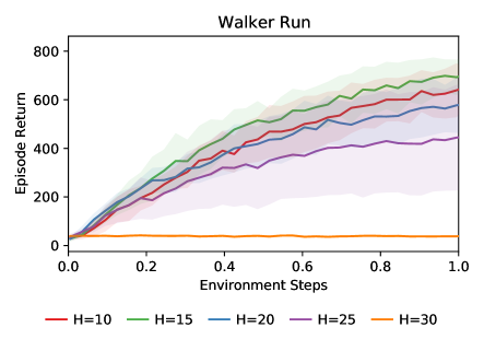
Figure 1: The learning curves of Dreamer (Hafner et al. 2019a) with different rollout horizons $H$ on the task of Walker Run. The solid lines depict the mean scores and shaded areas indicate the standard deviation of five trials over different random seeds. Each trial is evaluated every 10,000 environment steps. When applying relatively large $H$ (e.g. $H=30$), Dreamer fails to learn a good policy on this task. Results indicate that the performance of Dreamer is sensitive to the setting of $H$.

Many of the existing model-based RL methods hope to obtain more accurate value estimation by incorporating multi-horizon rollouts, but the rollout length is fixed to the maximum setting. For example, STEVE (Buckman et al. 2018) leverages model ensembles to dynamically interpolating between different rollouts. Selective MVE (Zaheer et al. 2020) incorporates learned variance into planning aside from model ensembles. However, none of these works focuses on visual control tasks. When dealing with pixel input problems, approaches like STEVE may be computationally expensive. Dreamer (Hafner et al. 2019a) focuses on visual control tasks. It also incorporates multi-horizon rollouts with fixed length by utilizing latent imagination. A demonstration of the relationship between the maximum rollout horizon selection and policy learning is illustrated in Figure 1. We evaluate the performance of Dreamer (Hafner et al. 2019a) on a classic task of DeepMind Control Suite (Tassa et al. 2020) Walker Run. It can be seen that different rollout horizons have a great impact on the performance of the algorithm. Results indicate that while multi-step information can be integrated, the rollout horizon itself is still essential for model-based planning. Therefore, in this paper, we argue that more accurate value estimation can be gained by dynamically adjusting the rollout horizon of the model, and a state-related adaptive horizon should be given within the maximum.

To deal with the influence of model inaccuracies, one natural solution is to incorporate uncertainty into the prediction of the world model. Although model ensembles can be used to measure model uncertainty (Rajeswaran et al. 2017; Kurutach et al. 2018; Clavera et al. 2018), they are not very suitable for visual control tasks due to the large computational burden. Intuitively, the uncertainty of the model and the novelty of data is highly relevant. In deep learning methods, when the new images are fed into the encoder-decoder models, these models tend to be ineffective and have significant reconstruction errors. Thus, the reconstruction error is considered as a measure of visual data novelty (Pimentel et al. 2014; Sabokrou et al. 2018; Denouden et al. 2018). Inspired by novelty detection with reconstruct-based approaches, the reconstructed images are used to determine the adaptive horizons for more accurate value estimation in our method.

In this paper, we propose Dynamic-horizon Model-based Value Expansion (DMVE), which adjusts the world model usage for value estimation through adaptive rollout horizons selection. In order to estimate state values, DMVE first adopts a reconstruction network to rebuild the original observation. Subsequently, the raw and reconstructed images are both fed into the transition module to imagine in the latent space, and the value expansion is calculated with diverse imagination horizons for both. Afterward, the horizons corresponding to the top minimum value expansion errors between the original image and the reconstructed image are selected, and the final value estimation is averaged from the expansion values corresponding to the selected horizons. Experimental results demonstrate that DMVE achieves higher sample efficiency and better asymptotic performance than baseline methods (Mnih et al. 2016; Barth-Maron et al. 2018; Hafner et al. 2019a, b).

The contributions of our work are summarized as follows:

• We develop an algorithm introducing Latent Imagination into Model-based Value Expansion (MVE-LI) and leverages advanced value estimation and policy learning objectives for visual control tasks.

• We propose a novel method named DMVE, which can dynamically adjust the world model usage through adaptive rollout horizons selection. Furthermore, various experiments are designed to better understand the overall performance gained by the proposed algorithm.

2 Related Work

To solve reinforcement learning problems, the Policy Gradient (PG) methods are aimed at modeling and optimizing the policy directly. REINFORCE (Williams 1992) is a classical PG method that relies on an estimated return by using episode samples to update the policy. In order to reduce gradient variance in vanilla policy gradients, many methods adopt actor-critic model to learn a value function in addition to the policy. For example, the critics in A3C (Mnih et al. 2016) learn the value function while multiple actors are trained in parallel. DDPG (Lillicrap et al. 2015) combines DPG (Silver et al. 2014) with deep neural networks to learn a deterministic policy by experience replay. D4PG (Barth-Maron et al. 2018), an extension of DDPG, utilizes distributed parallel actors, distributional critic, multi-step returns, and prioritized experience replay. TD3 (Fujimoto, Hoof, and Meger 2018) is another variant of DDPG that applies clipped double Q-learning, delayed update, and target policy smoothing. SAC (Haarnoja et al. 2018) incorporates the entropy measure of the policy into the reward to encourage exploration. However, above methods fail to take advantage of gradients through transitions and simply maximize immediate values. In this work, our algorithm DMVE also employs the actor-critic model but it is in a model-based manner.

Model-based reinforcement learning approaches intend to improve sample efficiency by learning a dynamics model to simulate the environment (Sutton and Barto 2018). For instance, VPN (Oh, Singh, and Lee 2017), MVE (Feinberg et al. 2018), and Dreamer (Hafner et al. 2019a) use the imagination of a learned model to assist the target value estimation. Dyna (Sutton 1991) and I2A (Racanière et al. 2017) learn dynamics to provide supplementary context for policy learning. Nevertheless, the model error has an inclination to harm the planning of model-based approaches, which is also known as model-bias (Deisenroth and Rasmussen 2011). This work is mainly based on the framework of Dreamer but we take the world model usage into account.

Previous works also explore the model usage to deal with model-bias by considering the uncertainty of the learned model. STEVE (Buckman et al. 2018) extends MVE by dynamically interpolating between model rollouts of various horizon lengths for each individual example. MBPO (Janner et al. 2019) as well as BMPO (Lai et al. 2020) combines model ensembles with short model rollouts for sufficient policy optimization. Selective MVE (Zaheer et al. 2020) incorporates learned variance into planning to use the model selectively. There are several world model architecture alternatives, such as linear models (Parr et al. 2008; Sutton et al. 2012; Levine and Abbeel 2014; Kumar, Todorov, and Levine 2016), Gaussian processes (Kuss and Rasmussen 2004; Ko et al. 2007), and neural networks (Draeger, Engell, and Ranke 1995; Nagabandi et al. 2018). World Models (Ha and Schmidhuber 2018) learn latent dynamics to help evolve linear controllers. PlaNet (Hafner et al. 2019b) learns world model components jointly and uses them to planning on latent space. In this work, DMVE utilizes the world model architecture in PlaNet (Hafner et al. 2019b).

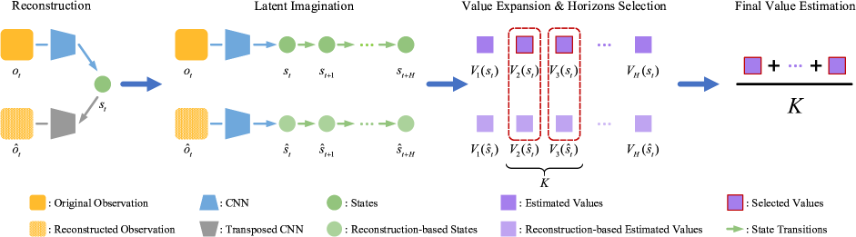
Figure 2: The overview of DMVE. To estimate state values, DMVE first adopts a reconstruction network to reconstruct the original observation. Then the raw and reconstructed images are both fed into the transition module to do $H$-step latent imagination, and the value expansion is calculated with diverse rollout horizons $h=1,2,\cdots,H$ for both. Afterward, the horizons corresponding to the top $K$ minimum value expansion errors between the original image and the reconstructed image are selected. Finally, the value estimation is averaged from the expansion values corresponding to the selected horizons.

3 Preliminaries

3.1 POMDP and RL

In this paper, the task of visual control is formulated as a Partially Observable Markov Decision Process (POMDP) since the agent cannot directly observe the underlying states on this kind of task. POMDP is a generalization of Markov Decision Process (MDP), which connects unobservant system states to observations. Formally, it can be described as a 7-tuple $\left(\mathcal{S},\mathcal{A},\mathcal{O},T,R,P,\gamma\right)$, where $\mathcal{S}$ denotes the set of states, $\mathcal{A}$ denotes the set of actions, and $\mathcal{O}$ denotes the set of observations. The agent interacts with the environment at each of a sequence of discrete time steps, $t=0,1,\cdots$. $T\left(s_{t+1}|s_{t},a_{t}\right)$ is the conditional transition probability that action $a_{t}\in\mathcal{A}$ in state $s_{t}\in\mathcal{S}$ will lead to state $s_{t+1}$. $R(s_{t},a_{t})$ yields the real-valued reward for executing action $a_{t}$ in state $s_{t}$ and $P$ denotes the observation probabilities $P(o_{t}|s_{t+1},a_{t})$, where $o_{t}$ stands for the observation made by the agent, when action $a_{t}$ is executed and the world moved to the state $s_{t+1}$. $\gamma\in(0,1)$ is a discount factor.

The policy $\pi(s)$ maps from environmental states to actions. At each time step $t$, the environment is in some state $s_{t}\in\mathcal{S}$, and the agent selects a feasible action $a_{t}\in\mathcal{A}$ in one state, which causes the environment to transition to state $s_{t+1}\in\mathcal{S}$ with probability $T\left(s_{t+1}|s_{t},a_{t}\right)$. After the action carried out in the environment, the agent receives an observation $o_{t}\in\mathcal{O}$ with probability $P(o_{t}|s_{t+1},a_{t})$ and a numerical reward $R(s_{t},a_{t})$. Then the above interaction process repeats. The goal of RL is to learn an optimal policy by maximizing the cumulative reward (Sutton and Barto 2018),

$$\max\mathbb{E}\left[{\sum\limits_{t=0}^{\infty}{{\gamma^{t}}R\left({{s_{t}},{a_{t}}}\right)}}\right].$$ (1)

3.2 MVE

Model-based Value Expansion (MVE; Feinberg et al. 2018) utilizes a learned dynamics model to enhance value estimates, hoping to improve both the sample efficiency and performance.

Using the imagined states $\{s_{t+n}\}_{n=1}^{H}$ (where $H$ denotes the finite maximum rollout horizon) obtained from the world model, the $H$-step value expansion of a given state $s_{t}$ can be estimated with

$${V_{H}}({s_{t}})=\sum\limits_{n=0}^{H-1}{{\gamma^{n}}{r_{t+n}}}+{\gamma^{H}}v({s_{t+H}}),$$ (2)

where $v(s)$ denotes the value function and $r$ denotes a state-related reward function.

Algorithm 1 Dynamic-horizon Model-based Value Expansion (DMVE)

1:Initialization: Number of random seed episodes $S$, collect interval $C$, batch size $B$, sequence length $L$, maximum imagination horizon $H$, learning rate $\alpha$, and number of selected horizons $K$

2:Collect dataset $\mathcal{D}$ with $S$ episodes through the interaction with the environment ENV using random actions

3:Initialize world model $w_{\theta}$, actor network $\pi_{\phi}$, critic network $v_{\psi}$

4:while not converged do

5:     for $c=1,\cdots,C$ do

6:         Sample $B$ data sequences $\left\{{\left({{a_{t}},{o_{t}},{r_{t}}}\right)}\right\}_{t=k}^{k+L}\sim\mathcal{D}$ and derive model states $s_{t}\sim w_{\theta}^{S}\left(s_{t}|s_{t-1},a_{t-1},o_{t}\right)$

7:         Update $\theta$ using representation learning

8:         Compute the reconstructed observations ${\hat{o}_{t}}\sim w_{\theta}^{O}\left({{\hat{o}_{t}}|{s_{t}}}\right)$ and reconstruction-based states $\hat{s}_{t}\sim w_{\theta}^{S}\left(\hat{s}_{t}|s_{t-1},a_{t-1},\hat{o}_{t}\right)$

9:         Estimate state values $V_{h}({s_{t}})$ and $V_{h}({\hat{s}_{t}})$ following Eq. (9) for $h=1,\cdots,H$

10:         Select $K$ horizons via Eq. (10) and determine final value estimation $V({s_{t}})$ via Eq. (11)

11:         Update actor network parameters $\phi\leftarrow\phi+\alpha{\hat{\nabla}_{\phi}}J_{\pi}\left(\phi\right)$

12:         Update critic network parameters $\psi\leftarrow\psi-\alpha{\hat{\nabla}_{\psi}}J_{v}\left(\psi\right)$

13:     end for

14:     ${o_{1}}\leftarrow\text{ENV.reset}\left(\right)$

15:     for $t=1,\cdots,T$ do

16:         Compute $s_{t}\sim w_{\theta}^{S}\left(s_{t}|s_{t-1},a_{t-1},o_{t}\right)$ from history and $a_{t}\sim\pi_{\phi}(a_{t}|s_{t})$ with the actor network

17:         Add exploration noise to action and take it in environment to get ${r_{t},o_{t+1}}\leftarrow\text{ENV.step}\left(a_{t}\right)$

18:     end for

19:     Add experience to dataset $\mathcal{D}\leftarrow\mathcal{D}\cup\left\{{\left({{a_{t}},{o_{t}},{r_{t}}}\right)}\right\}_{t=1}^{T}$

20:end while

4 Methodology

In this section, we present the framework of DMVE and further introduce how DMVE dynamically adjusts the world model usage. The overall architecture is illustrated in Figure 2, and the pseudocode is shown in Algorithm 1.

4.1 MVE by Latent Imagination

We first present our framework backbone, an MVE-like algorithm that takes advantage of a world model, an action model, and a value model to estimate state values. MVE is proposed by Feinberg et al. (2018) which builds a dynamics model and uses its imagination as the context for value estimation (see Section 3.2). Here, we extend MVE to visual control tasks by adopting latent imagination (Hafner et al. 2019a), and refer to this algorithm as MVE-LI (where LI stands for Latent Imagination) in this paper.

World Model

Many model-based RL methods first build a world model and further use it to derive behaviors. In the case that the world model is learned, the process of model learning and policy learning can be alternately paralleled. Usually, the world model provides the dynamics of a system, mapping from current state and action to the next state and giving rewards for this transition. There are several world model alternatives having the ability to be applied to visual control tasks, we choose the one used in PlaNet (Hafner et al. 2019b) and Dreamer (Hafner et al. 2019a) since it learns dynamics for planning by reconstructing the original images. At the same time, this reconstruction-based architecture is suitable for dynamic horizons selection (see Section 4.2). The world model $w_{\theta}$ is made up of the following components,

$$\begin{aligned} &\text{Representation module:}&&s_{t}\sim w_{\theta}^{S}\left(s_{t}|s_{t-1},a_{t-1},o_{t}\right)\\ &\text{Reconstruction module:}&&\hat{o}_{t}\sim w_{\theta}^{O}\left(\hat{o}_{t}|s_{t}\right)\\ &\text{Reward module:}&&r_{t}\sim w_{\theta}^{R}\left(r_{t}|s_{t}\right)\\ &\text{Transition module:}&&s_{t}\sim w_{\theta}^{T}\left(s_{t}|s_{t-1},a_{t-1}\right),\end{aligned}$$ (3)

where $\hat{o}_{t}$ denotes the reconstructed observation of time step $t$.

In the POMDP setting, states cannot be obtained directly, the representation module is thus applied to map the observations with actions to low-dimensional continuous vectors that are regarded as the states of Markovian transitions (Watter et al. 2015; Zhang et al. 2019; Hafner et al. 2019a, b). The reconstruction module estimates the original observations from the states and ensures that the states can represent effective information in the raw input data by minimizing the reconstruction error. The reward module predicts the rewards in the imaginary trajectories based on the real-value rewards from the environmental feedback. And the transition module predicts the next state purely depending on the current state and action without seeing the raw observation. In this work, the transition module is implemented as a Recurrent State Space Model (RSSM; Hafner et al. 2019b). The representation module is a combination of the RSSM and a Convolutional Neural Network (CNN; LeCun et al. 1989). The reconstruction module is a transposed CNN, and the reward module is a dense network. All four model components are optimized jointly through stochastic backpropagation, which is the same as Dreamer (Hafner et al. 2019a).

Policy Learning

We adopt an actor-critic method for policy learning. In addition to the estimated value function, actor-critic methods have an independent structure to represent the policy. The policy structure is known as the actor, since is used to derive behaviors. At the same time, the value function is called a critic because it criticizes the behaviors decided by the actor. For state $s_{t}$, the actor and critic models are defined as,

$$\begin{aligned} &\text{Actor:}&&a_{t}\sim\pi_{\phi}(a_{t}|s_{t})\\ &\text{Critic:}&&v_{\psi}({s_{t}})\approx{\mathbb{E}_{\pi(\cdot|{s_{t}})}}\left({\sum\limits_{\tau=t}^{t+H}{{\gamma^{\tau-t}}{r_{\tau}}}}\right),\end{aligned}$$ (4)

In this work, the actor and critic models are both implemented as dense networks (Hafner et al. 2019a). State values need to be estimated for the actor and critic models optimization. MVE can improve value estimation by assuming an approximate dynamics model and a reward function. Since the aforementioned world model contains the elements needed for value expansion, we can use it to estimate state values. While several approaches can be adopted, MVE-LI uses the classic value expansion introduced in MVE paper (Feinberg et al. 2018, see Section 3.2) . Selecting one $h\in\{1,2,\cdots,H\}$, we can compute the value estimation of $s_{t}$ with imagined trajectories $\left\{{\left({{s_{t+n}},{a_{t+n}},{r_{t+n}}}\right)}\right\}_{n=0}^{H}$ using

$$\begin{aligned} V_{h}({s_{t}})&=V(s_{t},h)\\ &={\mathbb{E}_{{w_{\theta}},{\pi_{\phi}}}}\left(\sum\limits_{n=0}^{h-1}{{\gamma^{n}}{r_{t+n}}+{\gamma^{h}}{v_{\psi}}({s_{t+h}})}\right),\end{aligned}$$ (5)

where the expectation is estimated under the imagination.

In MVE-LI, the imagination horizon is fixed to the maximum $H$. Therefore, the estimated value for state $s_{t}$ can be represented as $V_{H}({s_{t}})$. After estimating the state values, the actor and critic neural networks can be optimized while the world model is fixed. The learning objectives of the actor and critic models in MVE-LI are set as,

$${J_{\pi}}(\phi) =\mathop{\max}\limits_{\phi}{\mathbb{E}_{{w_{\theta}},{\pi_{\phi}}}}\left({\max{{\left\{{{V_{h}}({s_{t}})}\right\}}_{h=1,2,\cdots,H}}}\right),$$ (6)

$${J_{v}}(\psi) =\mathop{\min}\limits_{\psi}{\mathbb{E}_{{w_{\theta}},{\pi_{\phi}}}}\left({\frac{1}{2}{{\left\|{{v_{\psi}}({s_{t}})-{V}({s_{t}})}\right\|}^{2}}}\right),$$ (7)

where the estimated value ${V}({s_{t}})={V_{H}}({s_{t}})$ for MVE-LI.

4.2 Dynamic Horizon Value Estimation

The developed MVE-LI imagines future states in the latent space with a fixed maximum rollout horizon $H$. However, for different imagination horizons $h\in\left\{1,2,\cdots,H\right\}$, we can estimate diverse values for state $s_{t}$,

$$V_{h}({s_{t}}),h\in\left\{1,2,\cdots,H\right\}.$$ (8)

This leads to the question of which $h$ is the most suitable for the current state $s_{t}$.

Basic Assumptions

A reconstruction model often relies on encoder-decoder deep neural networks to rebuild the input data. These networks usually design a hidden layer with a lower dimensionality than the original input, and are optimized to learn a compressed representation of the input data distribution. Therefore, these models have a tendency to be ineffective at encoding novel data and fail to reconstruct the input without significant error (Pimentel et al. 2014; Sabokrou et al. 2018; Denouden et al. 2018). Thus, the reconstruction error is considered as a measure of visual data novelty.

Coincidentally, in a model-based RL setting, the data novelty has the potential to influence the value estimation accuracy since the world model may fail to predict trustable future states of novel data. This inspired us to apply the reconstruction-based approaches to dynamically adjust the world model usage with different rollout horizons for different states. Based on the observation of novelty detection with reconstruction error, the output difference of a model between the original image and the reconstructed image may also reflect the generalization ability of the model on the current input. To sum up, we enumerate the basic assumptions of DMVE here,

• For MVE, the data novelty influences the value estimation accuracy;

• The output error between the original and the reconstructed images of the world model reflects the generalization of the model to the observation.

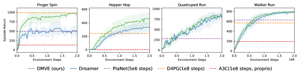
Figure 3: Comparison of DMVE (ours) and four baselines on different continuous visual control environments. The solid lines depict the mean scores and shaded areas indicate the standard deviation of five trials over different random seeds. Each trial is evaluated every 10,000 environment steps. The performance of D4PG, A3C, and PlaNet are taken directly from Dreamer paper.

Reconstruction-based Horizon Selection

Since we formulate the task of visual control as a POMDP problem, the original observations cannot fully characterize the states. Therefore, it is unreasonable to directly determine the imagination horizon with the reconstruction error. Based on the aforementioned assumptions, we now describe an algorithm using reconstructed images to do dynamic horizon value estimation.

Given the maximum rollout horizon $H$, we can get the value estimation $V_{h}$ with different $h\in\left\{1,2,\cdots,H\right\}$ for the data sequences ${\mathop{\left\{{\left({a_{t},o_{t},r_{t}}\right)}\right\}}\nolimits_{t=k}^{k+L}}$ using the world model, where $L$ denotes the sequence length. First, the state of time step $t$ can be derived using $s_{t}\sim w_{\theta}^{S}\left(s_{t}|s_{t-1},a_{t-1},o_{t}\right)$. Subsequently, the value of state $s_{t}$ can be estimated following

$$\begin{aligned} &\underbrace{\begin{aligned} s_{\tau}&\sim w_{\theta}^{T}\left(s_{\tau}|s_{\tau-1},a_{\tau-1}\right)\\ r_{\tau}&\sim w_{\theta}^{R}\left(r_{\tau}|s_{\tau}\right)\\ v_{\tau}&\sim v_{\psi}\left(s_{\tau}\right)\end{aligned}}_{\tau=t,t+1,\cdots,t+H}\\ V_{h}(&{s_{t}})=\sum\limits_{\tau=t}^{t+h-1}{{\gamma^{\tau-t}}{r_{\tau}}+{\gamma^{h}}{v_{\psi}}({s_{t+h}})}.\end{aligned}$$ (9)

Similarly, for the reconstructed image $\hat{o}_{t}\sim w_{\theta}^{O}\left(\hat{o}_{t}|s_{t}\right)$, the reconstruction-based state can be derived with $\hat{s}_{t}\sim w_{\theta}^{S}\left(\hat{s}_{t}|s_{t-1},a_{t-1},\hat{o}_{t}\right)$ and the corresponding value can be estimated by following the same process of Eq. (9). Now we have $V_{h}({s_{t}})$ as well as $V_{h}({\hat{s}_{t}})$ for $h=1,2,\cdots,H$. On top of that, given the number of selected horizons $K$, the set of rollout horizons $\mathcal{H}$ can be determined by

$$\begin{aligned} \mathcal{V}&={\left\{{\left|{{V_{h}}\left({{s_{t}}}\right)-{V_{h}}({{\hat{s}}_{t}})}\right|}\right\}_{h=1}^{H}}\\ \mathcal{H}&=top_{\arg\min}\left({\mathcal{V},K}\right),\end{aligned}$$ (10)

where the $top_{\arg\min}\left(\mathcal{V},K\right)$ operation means to get the set of $K$ indices corresponding to the top $K$ minimum values in set $\mathcal{V}$. Then the final value estimation of DMVE is

$$V({s_{t}})=\frac{1}{K}\sum\limits_{h\in\mathcal{H}}{{V_{h}}({s_{t}})}.$$ (11)

And now, the actor and critic models can be optimized following the learning objectives in (6) and (7), respectively.

In the above process of adaptive horizons selection, the original and the reconstructed images are fed into different world model components, to predict future sequence and perform value estimation, respectively. According to our assumptions, the output error of the world model between these images reflects its generalization ability of different inputs. As a result, the error between the estimated state values based on the two is used to determine the horizons of the final value estimation. For stability consideration, we set a hyperparameter $K$, which is the number of selected horizons. The evaluation of how this hyperparameter influences performance can be found in Section 5.2.

5 Experiments

Our experiments aim to study the following three primary questions: 1) How well does DMVE perform on benchmark reinforcement learning visual control tasks, comparing with state-of-the-art model-based and model-free methods? 2) What are the critical components of DMVE? 3) How do our design choices affect the performance?

5.1 Comparative Evaluation

In this section, we compare our method with prior baselines, and these methods represent the state-of-the-art in both model-free and model-based reinforcement learning. Specifically, for model-free methods, the baselines include A3C (Mnih et al. 2016) and D4PG (Barth-Maron et al. 2018). For model-based approaches, we compare against PlaNet (Hafner et al. 2019b), which directly uses the world model for planning rather than explicit policy learning, and Dreamer (Hafner et al. 2019a), learns long-horizon behaviors from images and leverages neural network dynamics for value estimation, which is highly related to our approach.

We evaluate DMVE and these baselines on 4 visual control tasks of the DeepMind Control Suite (Tassa et al. 2020), namely, Finger, Hopper, Quadruped, and Walker. These tasks provide various challenges, for examlpe, the Hoppe Hop task delivers a difficulty in terms of sparse rewards. Observations are images of shape $64\times 64\times 3$. Each episode lasts for 1000 time steps with random initial states.

In this section, the number of selected horizons $K$ is set to $3$. The comparison results are illustrated in Figure 3. Across diverse visual control tasks, our method DMVE learns faster than existing methods and achieves better asymptotic performance than previous model-based and model-free algorithms. Take the Finger Spin task as an example, DMVE exceeds Dreamer by a wide margin, and gains comparable performance at 2 million steps as that of D4PG at 100 million steps. On the Hopper Hop task that requires long-horizon credit assignment, DMVE surpasses all baselines as well. Our experiments indicate that DMVE can achieve more effective and accurate value estimation than state-of-the-art model-based method Dreamer.

5.2 Design Evaluation

To better understand where the performance of DMVE benefits, different experiments are designed to evaluate our algorithm.

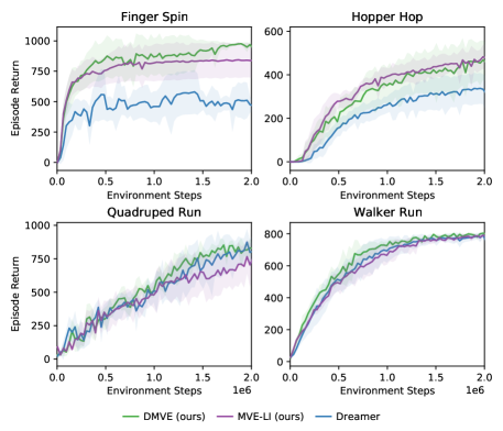
Figure 4: Comparison of DMVE and MVE-LI. The results are averaged from five trials. Each trial is evaluated every 10,000 environment steps.

Fixed Horizon

In this section, on the aforementioned experimental tasks, we first compare DMVE with our framework backbone MVE-LI which utilizes the same learning objectives but estimates state values with a fixed rollout horizon, to understand the contribution of the policy learning part and the dynamic horizon selection part of DMVE. The results are shown in Figure 4. Surprisingly, MVE-LI also surpasses Dreamer by a large margin in the Finger Spin and Hopper Hop tasks. However, on the tasks of Quadruped Run and Walker Run, its performance is not as good as Dreamer. It can be seen from the experimental results that our basic method MVE-LI uses advanced value estimation and policy learning objectives to achieve good results, and DMVE further improves the performance on its basis. And results indicate that the overall performance of DMVE benefits from two parts, one is the value estimation and the optimization of actor and critic networks, and the other is the dynamic rollout horizon selection for value estimation. Contributed by these two parts, DMVE basically achieves the best performance on the various challenging tasks according to our experiments. Although the learning efficiency is slightly reduced after adding dynamic horizon value estimation to the Hopper Hop task, the approximate best performance is finally obtained.

Value Estimation

In this work, we make use of a different value estimation from Dreamer (see Section 4.1). To be specific, Dreamer uses $V_{\lambda}$, that is,

$$\begin{aligned} V_{N}^{k}({s_{\tau}})&={\mathbb{E}_{{w_{\theta}},{\pi_{\phi}}}}\left({\sum\limits_{n=\tau}^{h-1}{{\gamma^{n-\tau}}{r_{n}}+}{\gamma^{h-\tau}}{v_{\psi}}\left({{s_{h}}}\right)}\right),\\ {V_{\lambda}}({s_{t}})&=\left({1-\lambda}\right)\sum\limits_{n=1}^{H-1}{{\lambda^{n-1}}V_{N}^{n}({s_{t}})+}{\lambda^{H-1}}V_{N}^{H}({s_{t}}),\end{aligned}$$ (12)

where $\tau=t,t+1,\cdots,t+H,h=\min\left({\tau+k,t+H}\right)$. We do not find incorporating $V_{\lambda}$ with DMVE works well because $V_{\lambda}$ itself integrates multi-horizon values. This reflects to a certain extent that it is more advantageous to select a suitable horizon adaptively for value estimation.

Hyperparameters Study

In this section, we study the question of how our design choices affect the performace of DMVE. We choose two key hyperparameters of our DMVE algorithm, namely, the maximum rollout horizon $H$, which is used in Eq. (9), and the number of selected horizons $K$, which appears in Eq. (10). To be specific, the hyperparameters of different experimental runs here are set as,

$$H=10,15,20,25,30, K=3,$$ (13)

$$K=1,3,5,7,9, H=15.$$ (14)

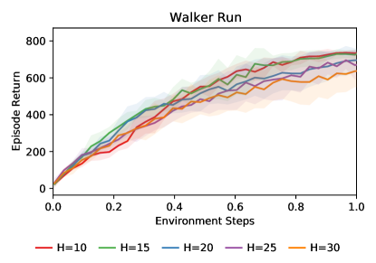
Figure 5: The learning curves of DMVE with different maximum imagination horizons $H$ on the task of Walker Run. The solid lines depict the mean scores and shaded areas indicate the standard deviation of five trials over different random seeds. Each trial is evaluated every 10,000 environment steps.

First, we evaluate DMVE with different $H$ ($K$ is fixed to $3$ here across different runs), and the results are shown in Figure 5. From the comparison between Figure 5 and Figure 1 (illustrated in Section 1), it is obvious that DMVE has better performance retention for various $H$ than Dreamer. When applying with long-horizon imagination (e.g. $H=30$), DMVE still can learn a relatively good policy on this task. This demonstrates the importance of adaptive horizon selection for value estimation, and policy learning.

In addition, we vary $K$ to investigate the sensitivity of DMVE to it ($H$ is fixed to $15$ across different runs). The results are plotted in Figure 6. We find that different $K$-value choices have some effect on the results, but overall DMVE can learn a good policy on the Walker Run task. Furthermore, we also find that although the number of selected horizons is diverse, the average value of horizons selected varies relatively little for different $K$, which reflects the stability of horizon selection with reconstruction-based methods. Moreover, the selection of multiple horizons also collects different horizon values into final value estimation like $V_{\lambda}$ does, but horizon selection works well with DMVE, not $V_{\lambda}$. One possible reason is that $V_{\lambda}$ incorporates long-horizon information even the maximum, which may harm the value estimation due to the model-bias. On the contrast, the horizons selected by DMVE are relatively small even with relatively large $K$ (e.g. $K=9$).

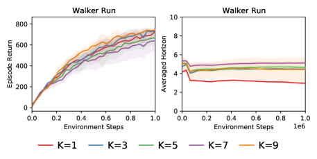
Figure 6: The learning curves and the averaged horizon curves of DMVE with different number of selected horizons $K$ on the task of Walker Run. The solid lines depict the mean scores and shaded areas indicate the standard deviation of five trials over different random seeds. Each trial is evaluated every 10,000 environment steps.

6 Conclusion

In this paper, we present an advanced method Dynamic-horizon Model-based Value Expansion (DMVE) which can adjust the world model usage for value estimation with adaptive state-related imagination horizons. We develop an algorithm which incorporates model-based value expansion with latent imagination. Also, an adaptive rollout horizon selection method is designed based on it. Experimental results indicate that DMVE outperforms state-of-the-art model-based method Dreamer on several benchmark visual control tasks. Since DMVE leverages reconstruction-based models that are limited to pixel inputs, our future work includes investigating the dynamic world model usage for state input tasks.

References

- Barth-Maron et al. (2018) Barth-Maron, G.; Hoffman, M. W.; Budden, D.; Dabney, W.; Horgan, D.; Dhruva, T.; Muldal, A.; Heess, N.; and Lillicrap, T. 2018. Distributed distributional deterministic policy gradients. In International Conference on Learning Representations.
- Buckman et al. (2018) Buckman, J.; Hafner, D.; Tucker, G.; Brevdo, E.; and Lee, H. 2018. Sample-efficient reinforcement learning with stochastic ensemble value expansion. In Advances in Neural Information Processing Systems, 8224–8234.
- Clavera et al. (2018) Clavera, I.; Rothfuss, J.; Schulman, J.; Fujita, Y.; Asfour, T.; and Abbeel, P. 2018. Model-based reinforcement learning via meta-policy optimization. In Conference on Robot Learning, 617–629.
- Deisenroth and Rasmussen (2011) Deisenroth, M.; and Rasmussen, C. E. 2011. PILCO: A model-based and data-efficient approach to policy search. In International Conference on Machine Learning, 465–472.
- Denouden et al. (2018) Denouden, T.; Salay, R.; Czarnecki, K.; Abdelzad, V.; Phan, B.; and Vernekar, S. 2018. Improving reconstruction autoencoder out-of-distribution detection with mahalanobis distance. arXiv preprint arXiv:1812.02765 .
- Draeger, Engell, and Ranke (1995) Draeger, A.; Engell, S.; and Ranke, H. 1995. Model predictive control using neural networks. IEEE Control Systems Magazine 15(5): 61–66.
- Feinberg et al. (2018) Feinberg, V.; Wan, A.; Stoica, I.; Jordan, M. I.; Gonzalez, J. E.; and Levine, S. 2018. Model-based value estimation for efficient model-free reinforcement learning. arXiv preprint arXiv:1803.00101 .
- Fujimoto, Hoof, and Meger (2018) Fujimoto, S.; Hoof, H.; and Meger, D. 2018. Addressing function approximation error in actor-critic methods. In International Conference on Machine Learning, 1587–1596.
- Ha and Schmidhuber (2018) Ha, D.; and Schmidhuber, J. 2018. Recurrent world models facilitate policy evolution. In Advances in Neural Information Processing Systems, 2450–2462.
- Haarnoja et al. (2018) Haarnoja, T.; Zhou, A.; Abbeel, P.; and Levine, S. 2018. Soft actor-critic: Off-policy maximum entropy deep reinforcement learning with a stochastic actor. In International Conference on Machine Learning, 1861–1870.
- Hafner et al. (2019a) Hafner, D.; Lillicrap, T.; Ba, J.; and Norouzi, M. 2019a. Dream to control: Learning behaviors by latent imagination. In International Conference on Learning Representations.
- Hafner et al. (2019b) Hafner, D.; Lillicrap, T.; Fischer, I.; Villegas, R.; Ha, D.; Lee, H.; and Davidson, J. 2019b. Learning latent dynamics for planning from pixels. In International Conference on Machine Learning, 2555–2565.
- Janner et al. (2019) Janner, M.; Fu, J.; Zhang, M.; and Levine, S. 2019. When to trust your model: Model-based policy optimization. In Advances in Neural Information Processing Systems, 12519–12530.
- Ko et al. (2007) Ko, J.; Klein, D. J.; Fox, D.; and Haehnel, D. 2007. Gaussian processes and reinforcement learning for identification and control of an autonomous blimp. In International Conference on Robotics and Automation, 742–747. IEEE.
- Kumar, Todorov, and Levine (2016) Kumar, V.; Todorov, E.; and Levine, S. 2016. Optimal control with learned local models: Application to dexterous manipulation. In International Conference on Robotics and Automation, 378–383. IEEE.
- Kurutach et al. (2018) Kurutach, T.; Clavera, I.; Duan, Y.; Tamar, A.; and Abbeel, P. 2018. Model-ensemble trust-region policy optimization. In International Conference on Learning Representations.
- Kuss and Rasmussen (2004) Kuss, M.; and Rasmussen, C. E. 2004. Gaussian processes in reinforcement learning. In Advances in Neural Information Processing Systems, 751–758.
- Lai et al. (2020) Lai, H.; Shen, J.; Zhang, W.; and Yu, Y. 2020. Bidirectional model-based policy optimization. arXiv preprint arXiv:2007.01995 .
- LeCun et al. (1989) LeCun, Y.; Boser, B.; Denker, J. S.; Henderson, D.; Howard, R. E.; Hubbard, W.; and Jackel, L. D. 1989. Backpropagation applied to handwritten zip code recognition. Neural computation 1(4): 541–551.
- Levine and Abbeel (2014) Levine, S.; and Abbeel, P. 2014. Learning neural network policies with guided policy search under unknown dynamics. In Advances in Neural Information Processing Systems, 1071–1079.
- Li et al. (2019) Li, D.; Zhao, D.; Zhang, Q.; and Chen, Y. 2019. Reinforcement learning and deep learning based lateral control for autonomous driving [application notes]. IEEE Computational Intelligence Magazine 14(2): 83–98.
- Li, Zhang, and Zhao (2019) Li, H.; Zhang, Q.; and Zhao, D. 2019. Deep reinforcement learning-based automatic exploration for navigation in unknown environment. IEEE transactions on Neural Networks and Learning Systems .
- Lillicrap et al. (2015) Lillicrap, T. P.; Hunt, J. J.; Pritzel, A.; Heess, N.; Erez, T.; Tassa, Y.; Silver, D.; and Wierstra, D. 2015. Continuous control with deep reinforcement learning. arXiv preprint arXiv:1509.02971 .
- Mnih et al. (2016) Mnih, V.; Badia, A. P.; Mirza, M.; Graves, A.; Lillicrap, T.; Harley, T.; Silver, D.; and Kavukcuoglu, K. 2016. Asynchronous methods for deep reinforcement learning. In International conference on Machine Learning, 1928–1937.
- Nagabandi et al. (2018) Nagabandi, A.; Kahn, G.; Fearing, R. S.; and Levine, S. 2018. Neural network dynamics for model-based deep reinforcement learning with model-free fine-tuning. In International Conference on Robotics and Automation, 7559–7566. IEEE.
- Oh, Singh, and Lee (2017) Oh, J.; Singh, S.; and Lee, H. 2017. Value prediction network. In Advances in Neural Information Processing Systems, 6118–6128.
- Parr et al. (2008) Parr, R.; Li, L.; Taylor, G.; Painter-Wakefield, C.; and Littman, M. L. 2008. An analysis of linear models, linear value-function approximation, and feature selection for reinforcement learning. In International Conference on Machine Learning, 752–759.
- Pimentel et al. (2014) Pimentel, M. A.; Clifton, D. A.; Clifton, L.; and Tarassenko, L. 2014. A review of novelty detection. Signal Processing 99: 215–249.
- Racanière et al. (2017) Racanière, S.; Weber, T.; Reichert, D.; Buesing, L.; Guez, A.; Rezende, D. J.; Badia, A. P.; Vinyals, O.; Heess, N.; Li, Y.; et al. 2017. Imagination-augmented agents for deep reinforcement learning. In Advances in neural information processing systems, 5690–5701.
- Rajeswaran et al. (2017) Rajeswaran, A.; Ghotra, S.; Ravindran, B.; and Levine, S. 2017. EPOpt: Learning robust neural network policies using model ensembles. In International Conference on Learning Representations.
- Sabokrou et al. (2018) Sabokrou, M.; Khalooei, M.; Fathy, M.; and Adeli, E. 2018. Adversarially learned one-class classifier for novelty detection. In Proceedings of the IEEE Conference on Computer Vision and Pattern Recognition, 3379–3388.
- Shao et al. (2018) Shao, K.; Zhao, D.; Li, N.; and Zhu, Y. 2018. Learning battles in vizdoom via deep reinforcement learning. In IEEE Conference on Computational Intelligence and Games, 1–4. IEEE.
- Shao, Zhu, and Zhao (2018) Shao, K.; Zhu, Y.; and Zhao, D. 2018. Starcraft micromanagement with reinforcement learning and curriculum transfer learning. IEEE Transactions on Emerging Topics in Computational Intelligence 3(1): 73–84.
- Silver et al. (2014) Silver, D.; Lever, G.; Heess, N.; Degris, T.; Wierstra, D.; and Riedmiller, M. 2014. Deterministic policy gradient algorithms. In International Conference on Machine Learning, 387–395.
- Sutton (1991) Sutton, R. S. 1991. Dyna, an integrated architecture for learning, planning, and reacting. ACM Sigart Bulletin 2(4): 160–163.
- Sutton and Barto (2018) Sutton, R. S.; and Barto, A. G. 2018. Reinforcement learning: An introduction. MIT press.
- Sutton et al. (2012) Sutton, R. S.; Szepesvári, C.; Geramifard, A.; and Bowling, M. P. 2012. Dyna-style planning with linear function approximation and prioritized sweeping. arXiv preprint arXiv:1206.3285 .
- Talvitie (2017) Talvitie, E. 2017. Self-correcting models for model-based reinforcement learning. In Proceedings of the Thirty-First AAAI Conference on Artificial Intelligence, 2597–2603.
- Tang et al. (2020) Tang, Z.; Zhu, Y.; Zhao, D.; and Lucas, S. 2020. Enhanced rolling horizon evolution algorithm with opponent model learning. IEEE Transactions on on Games doi:10.1109/TG.2020.3022698.
- Tassa et al. (2020) Tassa, Y.; Tunyasuvunakool, S.; Muldal, A.; Doron, Y.; Liu, S.; Bohez, S.; Merel, J.; Erez, T.; Lillicrap, T.; and Heess, N. 2020. dm_control: Software and tasks for continuous control. arXiv preprint arXiv:2006.12983 .
- Venkatraman, Hebert, and Bagnell (2015) Venkatraman, A.; Hebert, M.; and Bagnell, J. A. 2015. Improving multi-step prediction of learned time series models. In Proceedings of the Twenty-Ninth AAAI Conference on Artificial Intelligence, 3024–3030.
- Watter et al. (2015) Watter, M.; Springenberg, J.; Boedecker, J.; and Riedmiller, M. 2015. Embed to control: A locally linear latent dynamics model for control from raw images. In Advances in Neural Information Processing Systems, 2746–2754.
- Williams (1992) Williams, R. J. 1992. Simple statistical gradient-following algorithms for connectionist reinforcement learning. Machine Learning 8(3-4): 229–256.
- Zaheer et al. (2020) Zaheer, M.; Sokota, S.; Talvitie, E. J.; and White, M. 2020. Selective Dyna-style planning under limited model capacity. arXiv preprint arXiv:2007.02418 .
- Zhang et al. (2019) Zhang, M.; Vikram, S.; Smith, L.; Abbeel, P.; Johnson, M.; and Levine, S. 2019. SOLAR: Deep structured representations for model-based reinforcement learning. In International Conference on Machine Learning, 7444–7453.