The Volume of the Quiver Vortex Moduli Space

We study the moduli space volume of BPS vortices in quiver gauge theories on compact Riemann surfaces. The existence of BPS vortices imposes constraints on the quiver gauge theories. We show that the moduli space volume is given by a vev of a suitable cohomological operator (volume operator) in a supersymmetric quiver gauge theory, where BPS equations of the vortices are embedded. In the supersymmetric gauge theory, the moduli space volume is exactly evaluated as a contour integral by using the localization. Graph theory is useful to construct the supersymmetric quiver gauge theory and to derive the volume formula. The contour integral formula of the volume (generalization of the Jeffrey-Kirwan residue formula) leads to the Bradlow bounds (upper bounds on the vorticity by the area of the Riemann surface divided by the intrinsic size of the vortex). We give some examples of various quiver gauge theories and discuss properties of the moduli space volume in these theories. Our formula are applied to the volume of the vortex moduli space in the gauged non-linear sigma model with $\mathbb{C}P^{N}$ target space, which is obtained by a strong coupling limit of a parent quiver gauge theory. We also discuss a non-Abelian generalization of the quiver gauge theory and “Abelianization” of the volume formula.

1 Introduction

Vortices are co-dimension two solitons and play an important role for non-perturbative effects in gauge theories. In particular, the Bogomol’nyi-Prasad-Sommerfield (BPS) vortices appear as solutions to the BPS differential equations [1, 2] which minimize the energy of the Yang-Mills-Higgs system in three spacetime dimensions.

If the vortex equations are considered on compact Riemann surfaces $\Sigma_{h}$ with the genus $h$, the number of the vortices (vorticity) is restricted by an upper bound which is given by the finite area of $\Sigma_{h}$ divided by the intrinsic size of the vortex. This bound is called the Bradlow bound [3, 4].

Parameters of the vortex solutions are called moduli, and thier space is called the moduli space. (See for review [5, 6].) The structure of the moduli space is important to understand properties of the vortices themselves. The volume of the moduli space appears in the thermodynamics of the vortices [5, 7, 8, 9]. Since the thermodynamical partition function is proportional to the volume of the vortex moduli space, we can derive the free energy or equation of state from the volume. Although an integration of the volume form on the moduli space should give the volume of the moduli space, it is generally difficult to know the geometry of the moduli space, including the Kähler metric, except for some special cases [10]. (See also [5] for details.) On the other hand, the volume of the moduli space can be evaluated exactly without a detailed knowledge of the metric.

There are various way to obtain the volume of the moduli space. One way is to take advantage of the property of the moduli space as a Kähler manifold [8, 5]. To evaluate the volume by using the properties of the Kähler manifold, we need to know a topological structure of the moduli space like cohomologies or boundary divisors. The other way is to embed the BPS equation into supersymmetric gauge theory and to utilize the “localization” [11, 12, 13, 14, 15]. The localization method gives the volume as simple contour integrals even without knowing the geometry of the moduli space. In this sense, the localization method is universal and can be applied to any kind of the BPS equations in principle. In previous works [13, 14, 15], the volume of the moduli space of the vortex with a single $U(N_{c})$ gauge group and $N_{f}$ matters in the fundamental representation has been evaluated.

There have been a number of studies of vortices in gauge theories on curved manifolds, namely gauged nonlinear sigma models (GNLSM) [16, 17, 18, 19, 20, 21]. The GNLSM can be obtained if one considers a product of two gauge groups and matters charged under both of these gauge groups and takes a strong coupling limit of one of the gauge groups. Before taking the limit, we have linear gauged sigma model with a product of gauge groups and can be considered as a parent theory of GNLSM. Vortices in such theories with product gauge groups have also been studied before [22]. Gauge theories with a product of gauge groups and matters in bi-fundamental representations between two gauge groups are called quiver gauge theories. If we take a decoupling limit of a gauge group in the quiver gauge theory, where a gauge coupling constant goes to zero, the decoupled gauge group behaves as a global symmetry for the matters. So we can obtain the matters in the fundamental representation from the quiver gauge theory. Thus, the quiver gauge theory includes various types of the gauge theory in a very general form. Once a general formula for the volume of the vortex moduli space for the quiver gauge theory is derived, the BPS vortex equations with various kinds of matters or target space can be obtained. This is a strong motivation to consider the quiver gauge theory.

The quiver gauge theory can be realized by using the graph theory. The BPS vortices in the supersymmetric gauge theory on the graph has been studied in [23] inspired by the “deconstruction”. In addition, the quiver gauge theory naturally appears in the D-brane system of superstring theory. Open strings between D-branes give the gauge fields and bi-fundamental matters in the quiver gauge theory. Some of the quiver gauge theories can be realized as an effective theory on the D-branes at a tip of an orbifold. The volume of the vortex moduli space of quiver gauge theory can play an important role for non-perturbative effects in superstring theory.

The purpose of our paper is to obtain a formula for the volume of the moduli space of BPS vortices in quiver gauge theories on compact Riemann surfaces. We find that the graph theory in mathematical literature is useful to describe the quiver gauge theory. The gauge groups and bi-fundamental matters are expressed in terms of a directed graph (quiver diagram), which consists of the vertices and arrows (edges) connecting between the vertices. Each vertex represents a factor of the product gauge group, and each arrow gives the bi-fundamental matter, which transforms as fundamental and anti-fundamental representation for the gauge group at the source and target vertex of the arrow, respectively. Connection of vertices by edges in the graph is represented by a matrix called incidence matrix, which appears frequently in our construction of volume formulas for BPS vortices. Because of a zero left eigenvector of incidence matrix in a generic quiver gauge theories, the existence of BPS vortices imposes a stringent constraint on possible quiver gauge theories. We find two alternative solutions to the constraint. (i) All gauge groups have a common gauge coupling (universal coupling case). (ii) There is a gauge group whose gauge coupling vanishes (decoupled vertex case).

Embedding the vortex system into the supersymmetric quiver gauge theory, we define the supersymmetric transformation for the fields by a supercharge $Q$. Vacuum expectation values (vevs) of the cohomological operators, which is $Q$-closed but not $Q$-exact, is independent of the gauge coupling constants of the supersymmetric quiver gauge theory, since the action is $Q$-exact. So we can control the gauge coupling constants of the supersymmetric gauge theory without changing the vevs of the cohomological operators. If we take the controllable gauge coupling constants to the same value as the physical coupling constants in the BPS equations to evaluate the volume of the moduli space, the path integral is localized at the solution to the BPS equations. At the fixed points of the BPS solution, the matter (Higgs) fields take non-trivial value and the supersymmetric quiver gauge theory is in the Higgs branch. In the Higgs branch, we can show that the volume of the vortex moduli space is given by the vev of a suitable cohomological operator called the volume operator.

On the other hand, if we tune the controllable coupling constants to special values, the vevs of the Higgs fields vanish at the fixed points and the supersymmetric quiver gauge theory is in the Coulomb branch. In the Coulomb branch, the evaluation of the vev of the volume operator reduces to simple contour integrals. Using the coupling independence of the vev, we expect that the contour integrals also give the volume of the vortex moduli space as well as in the Higgs branch. Thus we obtain the contour integral formula of the volume of the vortex moduli space in the quiver gauge theory. As concrete examples to apply the contour integral formula for the volume of the vortex moduli space, we consider various quiver gauge theory with Abelian vertices. We discuss the Abelian quiver gauge theory with two or three vertices. For the integral to converge, we need a suitable choice of contours, which reproduces exactly the Bradlow bounds. The derivation of the Bradlow bounds from the contour integral can be regarded as a generalization of the Jeffrey-Kirwan (JK) residue formula [25]. A similar connection between the Bradlow bounds and the JK residue formula is also considered and utilized in the calculation of the index on $S^{1}\times\Sigma_{h}$ [26, 27]. In some examples of the quiver gauge theory with multiple Abelian vertices, the moduli space becomes non-compact. So we need to introduce regularization parameters, which can be regarded as the twisted mass of the matters. After taking zero limits of the regularization parameters, we can see the divergences of the volume of the moduli space corresponding to the non-compactness of the moduli space.

We also apply the contour integral formula of the volume to a quiver gauge theory corresponding to the parent gauged linear sigma model of Abelian GNLSM with $\mathbb{C}P^{N}$ target space with $n$ flavors of charge scalar fields. When restricted to $N=n=1$, our result agrees with the previous result in [21], which uses an entirely different method. We can also take a strong coupling limit of one of the gauge couplings, which gives the volume of the vortex moduli space of the GNLSM. Moreover, our contour integral formula provides a new results for the moduli space volume of the BPS vortex in the GNLSM with the target space $\mathbb{C}P^{N}$ and its parent GLSM with an arbitrary number $n$ of charged scalar fields.

The localization method can be extended to the case of non-Abelian quiver gauge theories. Since the non-Abelian gauge groups reduce to a product of $U(1)$’s in the Coulomb branch, the contour integral is expressed in terms of the Cartan part of the non-Abelian gauge groups, and the non-Abelian vertices in the quiver graph decompose into Abelian vertices. This “Abelianization” [28, 29] occurs in the localization formula and the quiver graph, because of the decomposition of the non-Abelian vertices into Abelian vertices in the quiver graph. Even with the Abelianization in the localization formula, the explicit evaluation of the contour integral becomes complicated due to the Vandermonde determinant which characterizes the non-Abelian case. However, our formula gives in principle the volume of the vortex moduli space in any non-Abelian quiver gauge theories. The non-Abelian generalization of the volume of the vortex moduli space in the GNLSM is also discussed.

The organization of this paper is as follows. In Sect. 2, basics of the quiver gauge theory and graph theory are explained, and the BPS vortex equations are derived. In Sect. 3, the BPS vortex system is embedded into a supersymmetric quiver gauge theory, and the volume operator (a cohomological operator) is introduced to obtain the volume of the vortex moduli space in the Higgs branch. The contour integral formula for the moduli space volume is obtained from localization in the Coulomb branch. In Sect. 4, we give various examples of the quiver gauge theory up to three Abelian vertices. Moduli space volumes in Abelian quiver gauge theories are evaluated explicitly by performing the contour integral. In Sect. 5, the vortex moduli space of a gauged linear sigma model (the parent theory of GNLSM) is obtained. That of the GNLSM is also obtained by taking the strong coupling limit. In Sect. 6, the contour integral formula is generalized to the non-Abelian cases, and the “Abelianization” of the non-Abelian quiver diagram is found. The Sect. 7 is devoted to conclusion and discussions. In Appendix A, path-integral measure for moduli is discussed.

2 BPS Vortex in Quiver Gauge Theory

2.1 Quiver diagram and graph theory

Figure 1: An example of the quiver diagram.

A quiver diagram is expressed by a directed graph $\Gamma=(V,E)$, which consists of a set of vertices $V$ and a set of directed edges (arrows) $E$. We denote elements of $V$ and $E$ by $v$ and $e$, respectively. We depict an example of the quiver diagram in Fig. 1.

We denote the total number of the vertices and edges by $n_{E}$ and $n_{V}$, respectively. Each directed edge $e\in E$ connects from a source vertex $s(e)\in V$ to a target vertex $t(e)\in V$ (see Fig. 2), i.e. each directed edge is specified by an ordered pair of two vertices $e=(s(e),t(e))$.

Figure 2: A part of the quiver diagram of two vertices connected with an edge. The source and target of the arrow (edge) $e$ are denoted by $s(e)$ and $t(e)$, respectively.

To describe the quiver diagram, it is useful to introduce language of graph theory. The graph theory describes a structure of the (quiver) graph in terms of elements of matrices. In graph theory, there are various kinds of the matrices or objects which describe and manipulate the graph structure, but we here introduce some of them only, which will be used to construct the quiver gauge theory.

First of all, we introduce the incidence matrix. The incidence matrix $L$ maps from $V$ to $E$, i.e. $n_{V}\times n_{E}$ matrix, whose elements are defined by

$${L_{v}}^{e}=\begin{cases}+1&\text{if }s(e)=v\\ -1&\text{if }t(e)=v\\ 0&\text{otherwise}\end{cases}.$$ (2.1)

For example, if we make the incidence matrix for the graph depicted in Fig. 1, we obtain

$$L=\left(\begin{array}[]{rrrrr}1&0&1&0&0\\ {-}1&1&0&1&{-}1\\ 0&{-}1&{-}1&0&0\\ 0&0&0&{-}1&1\end{array}\right)$$ (2.2)

For generic quiver gauge theory, a sum of the elements in each column vanishes

$$\sum_{v}{L_{v}}^{e}=0,$$ (2.3)

namely the multiplication of a vector $(1,\cdots,1)$ from the left annihilates the incidence matrix $L$. We will show that this will give a stringent constraint on quiver gauge theories admitting BPS vortices. Once the incidence matrix is given, we can reproduce the directed graph (quiver diagram).

If we assign variables $\vec{x}=(x_{1},x_{2},\ldots,x_{n_{V}})$ on each vertex, the incidence matrix multipied to the vector becomes a difference operator

$$x^{v}{L_{v}}^{e}=x_{s(e)}-x_{t(e)},$$ (2.4)

where the repeated upper and lower indices are summed implicitly. This property will be important to our formulation in the following.

Secondly, let us consider the Laplacian matrix $\Delta$ defined by

$$\Delta_{vv^{\prime}}=\begin{cases}{\rm deg}(v)&\text{if }v=v^{\prime}\\ -A_{vv^{\prime}}&\text{if }v\neq v^{\prime}\end{cases},$$ (2.5)

where ${\rm deg}(v)$ represents the number of the edges which connect to the vertex $v$ and $A_{vv^{\prime}}$ is the number of edges from $v$ to $v^{\prime}$. ($A_{vv^{\prime}}$ is also called the adjacency matrix.) The Laplacian matrix is also constructed from a square of the incidence matrix, i.e. $\Delta\equiv LL^{T}$. Hence the Laplacian always has at least one zero eigenvalue with the eigenvector proportional to $(1,\cdots,1)$.

Using the example in Fig. 1, the Laplacian matrix is given by

$$\Delta=\left(\begin{array}[]{rrrr}2&-1&-1&0\\ -1&4&-1&-2\\ -1&-1&2&0\\ 0&-2&0&2\end{array}\right).$$ (2.6)

We can notice that the Laplacian matrix is a generalization of the Cartan matrix in the Lie algebra.

If we assign variables $\vec{x}=(x_{1},x_{2},\ldots,x_{n_{V}})$ on each vertex, we can see that an inner product with the Laplacian matrix reduces

$$\vec{x}\Delta\vec{x}^{T}=\sum_{e\in E}(x_{s(e)}-x_{t(e)})^{2},$$ (2.7)

which is a second order difference operator between vertices. This is a reason why $\Delta$ is called the Laplacian on the graph. The Laplacian matrix does not preserve the orientation of the edges. So the Laplacian matrix cannot reproduce the whole structure of the quiver diagram including the orientation of the edges.

2.2 Quiver gauge theory and vortices

The quiver gauge theory is defined via a quiver diagram. Unitary groups $U(N_{v})$ are assigned to each vertex $v$, where $N_{v}$ is a rank of the unitary group. The quiver gauge theory has a gauge symmetry of a product group $\prod_{v\in V}U(N_{v})$ with the gauge couplings $g_{v}$. The bi-fundamental matters (scalar fields) $H^{e}$ are associated with each edges $e$ and represented by $({\bf N}_{s(e)},\bar{\bf N}_{t(e)})$, namely $N_{s(e)}\times N_{t(e)}$ complex matrices.

The vortex is a codimension two solitonic object, which appears as a classical static solution in $2+1$-dimensions. The vortex solution minimizes the “energy” of the $2+1$-dimensional system. To determine the energy, we first consider $2+1$-dimensional quiver Yang-Mills-Higgs theory on $M_{3}=\mathbb{R}_{t}\times\Sigma_{h}$. The metric on $M_{3}$ is given by

$$ds_{2+1}^{2}=-dt^{2}+2g_{z{\bar{z}}}dz\otimes d{\bar{z}}.$$ (2.8)

On the Riemann surface $\Sigma_{h}$, there exists a volume form $\omega=\sqrt{g}dz\wedge d{\bar{z}}$. An area of the Riemann surface ${\cal A}$ is given by an integral of the volume form

$${\cal A}=\int_{\Sigma_{h}}\omega.$$ (2.9)

For each gauge vertex $v$, there is gauge vector 1-form field $A_{(3)}^{v}=A^{v}_{0}dt+A^{v}_{z}dz+A^{v}_{\bar{z}}d{\bar{z}}$ on $M_{3}$. The field strength on $M_{3}$ is given by

$$F_{(3)}^{v}=d_{(3)}A_{(3)}^{v}+iA_{(3)}^{v}\wedge A_{(3)}^{v},$$ (2.10)

where $d_{(3)}$ is the exterior derivative on three-dimensional manifold $M_{3}$. On the other hand, on each edge $e$, we can assign a covariant derivative of the scalar field $H^{e}$

$$d^{(3)}_{A}H^{e}\equiv d_{(3)}H^{e}+iA^{s(e)}H^{e}-iH^{e}A^{t(e)}.$$ (2.11)

The action is written in terms of the quiver diagram by

$$\begin{split}S_{(3)}&=-\int_{\mathbb{R}_{t}\times\Sigma_{h}}\Bigg{[}\sum_{v\in V}\operatorname{Tr}_{v}\bigg{\{}\frac{1}{g_{v}^{2}}F^{v}_{(3)}\wedge*F^{v}_{(3)}\\ &\qquad\qquad\qquad\qquad+\frac{g_{v}^{2}}{4}\Big{(}\zeta^{v}{\bf 1}_{N_{v}}-\sum_{e:\,s(e)=v}H^{e}\bar{H}^{e}+\sum_{e:\,t(e)=v}\bar{H}^{e}H^{e}\Big{)}^{2}dt\wedge\omega\bigg{\}}\\ &\qquad\qquad\qquad\qquad\qquad+\sum_{e\in E}\operatorname{Tr}_{s(e)}d_{A}^{(3)}H^{e}\wedge{*}d_{A}^{(3)}\bar{H}^{e}\Bigg{]},\end{split}$$ (2.12)

where $\operatorname{Tr}_{v}$ stands for a trace over the rank $N_{v}$ gauge group at the vertex $v$, and the sum $\sum_{e:\,s(e)=v}$ ($\sum_{e:\,t(e)=v}$) is taken over edges whose sources (targets) are given by $v$.

Taking a static configuration and $A_{0}=0$ gauge, the gauge vector field reduces to (1,0)-form $A^{v}=A^{v}_{z}dz$ and (0,1)-form $\bar{A}^{v}=A_{\bar{z}}d{\bar{z}}$ on $\Sigma_{h}$, where the field strength (magnetic field) is given by

$$F^{v}=\partial\bar{A}^{v}+\bar{\partial}A^{v}+i(A^{v}\wedge\bar{A}^{v}+\bar{A}^{v}\wedge A^{v}),$$ (2.13)

where $\partial$ and $\bar{\partial}$ are the Dolbeault operators on $\Sigma_{h}$. Introducing a “metric”

$$G_{vv^{\prime}}=\frac{1}{g_{v}^{2}}\delta_{vv^{\prime}},\quad G_{ee^{\prime}}=\delta_{ee^{\prime}},$$ (2.14)

on $v$ and $e$, respectively, to raise and lower the indices, the energy is given by

$$\begin{split}E&=\int_{\Sigma_{h}}\operatorname{Tr}\Bigg{[}\mu_{v}\wedge{*}\mu^{v}+\frac{1}{2}\nu_{e}\wedge{*}\bar{\nu}^{e}+g_{v}^{2}\zeta_{v}F^{v}\Bigg{]}\\ &\geq 2\pi g_{v}^{2}\zeta_{v}k^{v},\end{split}$$ (2.15)

discarding the total divergence, where $\operatorname{Tr}$ is taken over suitable size of each term (gauge groups), and magnetic flux (first Chern class) for each gauge vertices is defined as

$$\frac{1}{2\pi}\int_{\Sigma_{h}}\operatorname{Tr}F^{v}=k^{v}\in\mathbb{Z}.$$ (2.16)

We have introduced here

$$\mu^{v} = F^{v}-\frac{g_{v}^{2}}{2}\Big{(}\zeta^{v}{\bf 1}_{N_{v}}-\sum_{e:\,s(e)=v}H^{e}\bar{H}^{e}+\sum_{e:\,t(e)=v}\bar{H}^{e}H^{e}\Big{)}\omega,$$ (2.17)

$$\nu^{e} = 2\partial_{A}\bar{H}^{e},$$ (2.18)

$$\bar{\nu}^{e} = 2\bar{\partial}_{A}H^{e},$$ (2.19)

where ${\bf 1}_{N_{v}}$ stands for a $N_{v}\times N_{v}$ unit matrix, and

$$\begin{split}\partial_{A}\bar{H}^{e}&\equiv\partial\bar{H}^{e}-i\bar{H}^{e}A^{s(e)}+iA^{t(e)}\bar{H}^{e},\\ \bar{\partial}_{A}H^{e}&\equiv\bar{\partial}H^{e}+i\bar{A}^{s(e)}H^{e}-iH^{e}\bar{A}^{t(e)}.\end{split}$$ (2.20)

The energy is saturated at a solution to the so-called BPS equations

$$\mu^{v}=\nu^{e}=\bar{\nu}^{e}=0.$$ (2.21)

We call the solution of the above differential equations on $\Sigma_{h}$ as the BPS vortex in the quiver gauge theory. Once we get the BPS equations, which minimize the energy (2.15), the equations (2.21) can be regarded just as the differential equations on two-dimensional $\Sigma_{h}$ and disregard the time direction. If we are interested in the solution to eqs. (2.21) and in the parameters of these solutions (moduli space), it is sufficient to consider the two-dimensional field theory on $\Sigma_{h}$ to embed the BPS equations. From this point of view, we will embed the BPS equations into the two-dimensional supersymmetric gauge theory.

Provided $g_{v}^{2}\not=0$, we can take a linear combination of $\mu^{v}$ weighted by $1/g_{v}^{2}$ to obtain

$$0=\sum_{v\in V}\frac{\mu^{v}}{g_{v}^{2}}=\sum_{v\in V}\left(\frac{F^{v}}{g_{v}^{2}}-\frac{\zeta^{v}}{2}{\bf 1}_{N_{v}}\omega\right),$$ (2.22)

because of the zero vector for incidence matrix in generic quiver gauge theory in Eq. (2.3). If we take the trace and integral over $\Sigma_{h}$, we find

$$\sum_{v\in V}\left(\frac{2\pi k^{v}}{g_{v}^{2}}-N_{v}\frac{\zeta^{v}{\cal A}}{2}\right)=0.$$ (2.23)

We will see that the integral formula for the volume of the moduli space gives a constraint identical to (2.23). Since $k^{v}$ are integer valued, this condition cannot be satisfied for the generic $g_{v}$ and $\zeta^{v}$. This means that the BPS vortices (solution) with $k^{v}\neq 0$ cannot exist on $\Sigma_{h}$ for the generic $g_{v}$ and $\zeta^{v}$. In fact, Eq. (2.23) gives a stringent restriction nolt only on parameters such as $g_{v}^{2}$ and $\zeta_{v}$ of the theory and also on allowed vorticity $k^{v}$ of BPS vortices.

First, the FI parameters $\zeta^{v}$ of the theory need to satisfy

$$\sum_{v\in V}N_{v}\zeta^{v}=0,$$ (2.24)

in order for vacuum ($k^{v}=0$ for all $v$) to exists.

In order to allow BPS states with nonzero vorticity, two types of solutions are available

1. Universal coupling:

   $$g_{1}=g_{2}=\cdots=g.$$ (2.25)

   The local constraint (2.22) at each point in space reduces in this case to

   $$\sum_{v\in V}F^{v}=0.$$ (2.26)

   Therefore the vorticity of $N_{v}-1$ gauge groups are no longer constrained. However, the gauge field of one of the gauge groups is completely determined (up to vacuum gauge field) by those of other gauge groups.

   As a more general solution with the universal coupling, we can consider the case $g_{v}^{2}=n_{v}g^{2}$ with $n_{v}\in{\mathbb{Z}}_{+}$. This solution allows not all but multiple of $n_{v}$ vorticity for each gauge group $v$.

   In sect.4 we consider the case of universal coupling.

2. Decoupled vertex:

   Another solution for the quiver gauge theories admitting BPS vortices is the case when there is at least one decoupled vertex $g_{v^{\prime}}=0$. The decoupled vertex gives only a global symmetry and no BPS condition arises for the $v^{\prime}$ vertex. The incidence matrix no longer posseses a zero vector, and the constraint (2.22) is absent. Hence we can have arbitrary coupling and FI parameters for other gauge groups, provided there is a decoupled vertex in the quiver diagram. We will consider such a case in sect.5.

3 Embedding into Supersymmetric Quiver Gauge Theory

We would like to consider the volume of the moduli space of the quiver BPS vortices, which are the solutions to the equations (2.21). It is useful to embed the system of the quiver BPS vortices into a supersymmetric quiver gauge theory, whose partition function is localized at the BPS solution.

The BPS vortex solution to the quiver BPS equations (2.21) involves the given gauge coupling constants $g_{v}$ as parameters. On the other hand, the embeded supersymmetric gauge theory has a gauge coupling constants $g_{0,v}$. The coupling constants $g_{0,v}$ appear as overall constants of the action of the supersymmetric quiver gauge theory and we will see that the partition function and vevs are independent of them, thanks to the localization theorem. Therefore we can choose $g_{0,v}$ differently from the “physical” gauge coupling $g_{v}$ in the BPS vortex. We will find that the coupling constants $g_{0,v}$ in the supersymmetric quiver gauge theory are controllable parameters which interpolate between the Higgs and Coulomb branch picture.

In the following subsections, we concentrate on the quiver gauge theory having only the Abelian vertices for a while, since it is sufficient to see the localization theorem and derivation of the volume of the moduli space. We will consider non-Abelian quiver gauge theories later. We will find that they can be treated by means of a decomposition of the non-Abelian vertices into the Abelian vertices.

3.1 Abelian vertices

Let us consider the supersymmetric quiver gauge theory which contains the Abelian vertices only, i.e. the total gauge group is $G=U(1)^{n_{V}}$.

On each vertex, there exist bosonic scalar fields $\phi^{v}$, gauge vector fields $A^{v}$, $\bar{A}^{v}$ and auxiliary fields $Y^{v}$, which are 0-forms, (1,0)-forms, (0,1)-forms and 2-forms on $\Sigma_{h}$, respectively. There also exist their superpartner fermions $\eta^{v}$, $\lambda^{v}$, $\bar{\lambda}^{v}$ and $\chi^{v}$, which are Grassmann-valued 0-forms, (1,0)-forms, (0,1)-forms and 2-forms on $\Sigma_{h}$, respectively. These bosons and fermions form vector multiplets of the Abelian gauge theory on each vertex.

The supersymmetric transformations between the vector multiplets are given by

$$\begin{array}[]{lcl}Q\phi^{v}=0,&&\\ Q\bar{\phi}^{v}=2\eta^{v},&&Q\eta^{v}=0,\\ QA^{v}=\lambda^{v},&&Q\lambda^{v}=-\partial\phi^{v},\\ Q\bar{A}^{v}=\bar{\lambda}^{v},&&Q\bar{\lambda}^{v}=-\bar{\partial}\phi^{v},\\ QY^{v}=0,&&Q\chi^{v}=Y^{v},\end{array}$$ (3.1)

where $\bar{\phi}^{v}$ is a complex conjugate of $\phi^{v}$. We note here that if we apply the $Q$ transformations twice on the fields, it generates a gauge transformation with a gauge parameter $\phi^{v}$, i.e. $Q^{2}=\delta_{\phi^{v}}$.

We also have chiral superfields on each edge. The chiral superfield consists of a complex scalar field $H^{e}$ and its fermionic partner $\psi^{e}$ of 0-form, and an auxiliary field $\bar{T}^{e}$ and its fermionic partner $\bar{\rho}^{e}$ of (0,1)-form, on the edge $e$. The chiral fields generally transform in the bi-fundamental representation, which means that they possess positive charges of a gauge group at the source of the edge $s(e)$ and negative charges at the target $t(e)$, for the Abelian gauge theory.

For those chiral superfields, the supersymmetric transformations are given by

$$\begin{array}[]{lcl}QH^{e}=\psi^{e},&&Q\psi^{e}=i\phi^{v}{L(H)_{v}}^{e},\\ Q\bar{T}^{e}=i{\phi^{v}L(\bar{\rho})_{v}}^{e},&&Q\bar{\rho}^{e}=\bar{T}^{e},\end{array}$$ (3.2)

which also satisfy $Q^{2}=\delta_{\phi^{v}}$. Here ${L(H)_{v}}^{e}$ is defined from the incidence matrix ${L_{v}}^{e}$ as

$$\begin{split}{L(H)_{v}}^{e}&\equiv{L_{v}}^{e}H^{e}\\ &=\begin{cases}+H^{e}&\text{if }v=s(e)\\ -H^{e}&\text{if }v=t(e)\\ 0&\text{others}\end{cases},\end{split}$$ (3.3)

and similarly ${L(\bar{\rho})_{v}}^{e}\equiv{L_{v}}^{e}\bar{\rho}^{e}$, where we do not take the sum for the repeated index $e$.

For their complex conjugate fields, which contain 0-form $(\bar{H}^{e},\bar{\psi}^{e})$, and (1,0)-form $(T^{e},\rho^{e})$, we have

$$\begin{array}[]{lcl}Q\bar{H}^{e}=\bar{\psi}^{e},&&Q\bar{\psi}^{e}=-i{L^{T}(\bar{H})^{e}}_{v}\phi^{v},\\ QT^{e}=-i{L^{T}(\rho)^{e}}_{v}\phi^{v},&&Q\rho^{e}=T^{e},\end{array}$$ (3.4)

where we defined ${L^{T}(\bar{H})^{e}}_{v}\equiv\bar{H}^{e}{{L^{T}}^{e}}_{v}$ and ${L^{T}(\rho)^{e}}_{v}\equiv\rho^{e}{{L^{T}}^{e}}_{v}$, without summing over the repeated edge index $e$, by using the transpose of the incidence matrix.

For later convenience, we introduce a norm between forms $\alpha$ and $\beta$ on $\Sigma_{h}$

$$\left\langle\alpha,\beta\right\rangle\equiv\int_{\Sigma_{h}}\alpha\wedge{*}\bar{\beta}.$$ (3.5)

Using this norm, the action for the vector multiplets on $v\in V$ is written as a $Q$-exact form

$$S_{V}=Q\Xi_{V},$$ (3.6)

where

$$\Xi_{V}=-\left[\langle\lambda_{v},\partial\phi^{v}\rangle+\langle\bar{\lambda}_{v},\bar{\partial}\phi^{v}\rangle+\langle\chi_{v},Y^{v}-2\mu_{0}^{v}\rangle\right].$$ (3.7)

A part of the BPS equations appears in the action (3.6);

$$\mu_{0}^{v}=F^{v}-\frac{g_{0,v}^{2}}{2}\Big{(}\zeta^{v}-\sum_{e:\,s(e)=v}H^{e}\bar{H}^{e}+\sum_{e:\,t(e)=v}\bar{H}^{e}H^{e}\Big{)}\omega,$$ (3.8)

which comes from the D-term constraint and is the same as $\mu^{v}$ in (2.17) for the original vortex system if we replace the coupling constants $g_{0,v}$ with $g_{v}$. We however need to distinguish between $\mu_{0}^{v}$ in the supersymmetric action and $\mu^{v}$ in the original quiver vortex BPS equations (2.17), since the solution includes the different coupling constants.

In the $Q$-exact action (3.6), the repeated lower-upper indices are summed implicitly and the raising or lowering of the indices, such as $\phi_{v}=G_{0,vv^{\prime}}\phi^{v^{\prime}}$, is given by a “metric” on the vertices

$$G_{0,vv^{\prime}}=\frac{1}{g_{0,v}^{2}}\delta_{vv^{\prime}},$$ (3.9)

which contains the gauge couplings $g_{0,v}$ in contrast to the metric (2.14). In this sense, the action (3.6) has the gauge couplings $g_{0,v}$ as an overall factor $1/g_{0,v}^{2}$.

Using the metric $G_{0,vv^{\prime}}$, we can rewrite eq. (3.8) as

$$\mu_{0}^{v}=F^{v}-\frac{1}{2}\Big{(}g_{0,v}^{2}\zeta^{v}-{L(H)^{v}}_{e}\bar{H}^{e}\Big{)}\omega,$$ (3.10)

where ${L(H)^{v}}_{e}=G_{0}^{vv^{\prime}}\delta_{ee^{\prime}}{L(H)_{v^{\prime}}}^{e^{\prime}}=g_{0,v}^{2}\delta^{vv^{\prime}}\delta_{ee^{\prime}}{L(H)_{v^{\prime}}}^{e^{\prime}}$, so ${L(H)^{v}}_{e}$ contains the coupling constants $g_{0,v}$ unlike ${L(H)_{v}}^{e}$.

For the chiral superfields, we can construct a $Q$-exact action given by

$$S_{C}=Q\Xi_{C},$$ (3.11)

where

$$\Xi_{C}=\frac{1}{2}\bigg{[}\langle\psi_{e},i\phi^{v}{L(H)_{v}}^{e}\rangle-\langle\bar{\psi}_{e},i{L^{T}(\bar{H})^{e}}_{v}\phi^{v}\rangle-\frac{1}{2}\langle\rho_{e},T^{e}-2\nu^{e}\rangle-\frac{1}{2}\langle\bar{\rho}_{e},\bar{T}^{e}-2\bar{\nu}^{e}\rangle\bigg{]}.$$ (3.12)

The constraints for the F-term conditions appear in the chiral superfields action (3.11) as;

$$\nu^{e} = 2\partial_{A}\bar{H}^{e},$$ (3.13)

$$\bar{\nu}^{e} = 2\bar{\partial}_{A}H^{e},$$ (3.14)

where

$$\begin{split}\partial_{A}\bar{H}^{e}&=\partial\bar{H}^{e}-i{L^{T}(\bar{H})^{e}}_{v}A^{v},\\ \bar{\partial}_{A}H^{e}&=\bar{\partial}H^{e}+i\bar{A}^{v}{L(H)_{v}}^{e},\end{split}$$ (3.15)

for the Abelian theory. Eqs. (3.13) and (3.14) are the same as the original ones (2.18) and (2.19) since they do not depend on the gauge couplings.

The raising or lowering of the indices of the edge $e$ is just given by $\delta_{ee^{\prime}}$, thus we can see the $Q$-exact action (3.11) does not contain any coupling constant $g_{0,v}$.

The total supersymmetric action is given by the sum of the vector and chiral multiplet parts

$$S=S_{V}+S_{C}.$$ (3.16)

By definition, the total action is also written in a $Q$-exact form

$$S=Q(\Xi_{V}+\Xi_{C}).$$ (3.17)

If we rescale the total action like

$$S\to tS,$$ (3.18)

the partition function or the vev of the supersymmetric operator ${\cal O}$, which satisfies $Q{\cal O}=0$, is independent of $t$, since the derivative with respect to $t$ reduces to the vev of the $Q$-exact operator and vanishes, i.e.

$$\frac{\partial}{\partial t}\left\langle{\cal O}\right\rangle_{t}=-\left\langle{\cal O}S\right\rangle_{t}=-\left\langle Q({\cal O}\Xi)\right\rangle_{t}=0,$$ (3.19)

where $\langle\cdots\rangle_{t}$ stands for the vev with the rescaled action $tS$. Note that we also find by a similar argument that the partition function or the vev of the supersymmetric operator is independent of the gauge coupling constants $g^{2}_{0,v}$ in $S_{V}$.

If we extract the bosonic part of the action from $S_{V}$ and $S_{C}$, we obtain

$$\begin{split}\left.S_{V}\right|_{B}&=\langle\partial\phi_{v},\partial\phi^{v}\rangle+\langle\bar{\partial}\phi_{v},\bar{\partial}\phi^{v}\rangle-\langle Y_{v},Y^{v}\rangle+2\langle Y_{v},\mu_{0}^{v}\rangle,\\ \left.S_{C}\right|_{B}&=\frac{1}{2}\bigg{[}\langle\phi^{v}L(H)_{ve},\phi^{v}{L(H)_{v}}^{e}\rangle+\langle L^{T}(\bar{H})_{ev}\phi^{v},{L^{T}(\bar{H})^{e}}_{v}\phi^{v}\rangle-\langle T_{e},T^{e}\rangle+\langle T_{e},\nu^{e}\rangle+\langle\nu_{e},T^{e}\rangle\bigg{]}.\end{split}$$ (3.20)

After integrating out the auxiliary fields $Y^{v}$ and $T^{e}$, we find

$$\begin{split}\left.S_{V}\right|_{B}&=\langle\partial\phi_{v},\partial\phi^{v}\rangle+\langle\bar{\partial}\phi_{v},\bar{\partial}\phi^{v}\rangle+\langle\mu_{0,v},\mu_{0}^{v}\rangle,\\ \left.S_{C}\right|_{B}&=\frac{1}{2}\bigg{[}\langle\phi^{v}L(H)_{ve},\phi^{v}{L(H)_{v}}^{e}\rangle+\langle L^{T}(\bar{H})_{ev}\phi^{v},{L^{T}(\bar{H})^{e}}_{v}\phi^{v}\rangle+\langle\nu_{e},\nu^{e}\rangle\bigg{]}.\end{split}$$ (3.21)

From the coupling independence, the path integral is localized at the fixed points which are determined by the equations

$$\mu_{0}^{v}=\nu^{e}=\bar{\nu}^{e}=0,$$ (3.22)

$$\partial\phi^{v}=\bar{\partial}\phi^{v}=0,$$ (3.23)

$$\phi^{v}{L(H)_{v}}^{e}={L^{T}(\bar{H})^{e}}_{v}\phi^{v}=0,$$ (3.24)

The equations in the first line (3.22) are the BPS equation for the quiver vortex at the gauge coupling $g_{0,v}$. The second line (3.23) and third line (3.24) show that the scalar fields $\phi^{v}$ take constant values on $\Sigma_{h}$, and $\phi^{v}$ and ${L(H)_{v}}^{e}$ are “orthogonal” with each other, respectively, at the fixed points. The orthogonality conditions (3.24) are solved either by $\langle\phi^{v}\rangle=0$ and $\langle H^{e}\rangle\neq 0$ (the Higgs branch point) or by $\langle\phi^{v}\rangle\neq 0$ and $\langle H^{e}\rangle=0$ (Coulomb branch point), leading to two distinct branches. Eqs. (3.24) can also contain special solutions in mixed branches ($\langle\phi^{v}\rangle\neq 0$ and $\langle H^{e}\rangle\neq 0$), where $\langle\phi^{v}\rangle$ is proportional to the vector annihilated by the incidence matrix. This mixed branch will be closely related to the constraints (2.22) in the derivation of the volume formula.

Finally, we here write down the fermionic part of the action

$$\begin{split}\left.S_{V}\right|_{F}&=2\langle\lambda_{v},\partial\eta^{v}\rangle+2\langle\bar{\lambda}_{v},\bar{\partial}\eta^{v}\rangle-2\left\langle\chi_{v},\partial\bar{\lambda}^{v}+\bar{\partial}\lambda^{v}+\frac{1}{2}\left(\psi^{e}{L^{T}(\bar{H})_{e}}^{v}+{L(H)^{v}}_{e}\bar{\psi}^{e}\right)\right\rangle,\\ \left.S_{C}\right|_{F}&=i\langle\psi_{e},\eta^{v}{L(H)_{v}}^{e}\rangle-i\langle\bar{\psi}_{e},{L^{T}(\bar{H})^{e}}_{v}\eta^{v}\rangle\\ &\qquad\qquad+\frac{i}{2}\langle\psi_{e},\phi^{v}{L(\psi)_{v}}^{e}\rangle-\frac{i}{2}\langle\bar{\psi}_{e},{L^{T}(\bar{\psi})^{e}}_{v}\phi^{v}\rangle\\ &\qquad\qquad\qquad+\frac{i}{4}\langle\rho_{e},{L^{T}(\rho)^{e}}_{v}\bar{\phi}^{v}\rangle-\langle\rho_{e},\partial_{A}\bar{\psi}^{e}-i{L^{T}(\bar{H})^{e}}_{v}\lambda^{v}\rangle\\ &\qquad\qquad\qquad\qquad-\frac{i}{4}\langle\bar{\rho}_{e},\bar{\phi}^{v}{L(\bar{\rho})_{v}}^{e}\rangle-\langle\bar{\rho}_{e},\bar{\partial}_{A}\psi^{e}+i\bar{\lambda}^{v}{L(H)_{v}}^{e}\rangle,\end{split}$$ (3.25)

for later discussions.

3.2 Higgs branch localization

Firstly, we consider the localization of the supersymmetric gauge theory in the Higgs branch, where the scalar fields $\phi^{v}$ vanish and the Higgs scalar $H^{e}$ and gauge fields $A^{v}$ take non-vanishing values in general.

Using the coupling independence of the supersymmetric theory, we can choose the controllable couplings to be $g_{0,v}=g_{v}$, where $g_{v}$ are the coupling constants appeared in the BPS quiver vortex equation which we would like to consider. After choosing the couplings in the Higgs branch, the fixed point equations (3.22) reduce to the BPS equations for the quiver vortex. Thus solutions to the localization fixed point equations are given by configurations of the quiver vortex.

We denote one of the quiver vortex solutions by $\hat{A}^{v}$, $\hat{\bar{A}}^{v}$, $\hat{H}^{e}$ and $\hat{\bar{H}}^{e}$. In the Higgs branch, the fields are expanded around this solution (fixed point) as

$$\begin{array}[]{lcl}A^{v}=\hat{A}^{v}+\frac{1}{\sqrt{t}}\tilde{A}^{v},&&\bar{A}^{v}=\hat{\bar{A}}^{v}+\frac{1}{\sqrt{t}}\tilde{\bar{A}}^{v},\\ H^{e}=\hat{H}^{e}+\frac{1}{\sqrt{t}}\tilde{H}^{e},&&\bar{H}^{e}=\hat{\bar{H}}^{e}+\frac{1}{\sqrt{t}}\tilde{\bar{H}}^{e}.\end{array}$$ (3.26)

Other bosonic and fermionic fields are expanded around vanishing backgrounds. We just rescale these fields like $\phi^{v}\to\phi^{v}/\sqrt{t}$.

We now introduce Faddeev-Popov ghosts $c^{v}$ and $\bar{c}^{v}$ and Nakanishi-Lautrup (NL) field $B^{v}$ on the vertices to fix the gauge. The BRST transformation, which is nilpotent $\delta_{B}^{2}=0$, is given by

$$\begin{split}&\delta_{B}\bar{c}^{v}=2B^{v},\\ &\delta_{B}c^{v}=\delta_{B}B^{v}=0,\end{split}$$ (3.27)

for the ghosts and NL fields,

$$\begin{split}\delta_{B}\tilde{A}^{v}&=-\partial c^{v},\\ \delta_{B}\tilde{\bar{A}}^{v}&=-\bar{\partial}c^{v},\\ \delta_{B}\tilde{H}^{e}&=ic^{v}{L(\hat{H})_{v}}^{e},\\ \delta_{B}\tilde{\bar{H}}^{e}&=-i{{L^{T}(\hat{\bar{H}})}^{e}}_{v}c^{v},\end{split}$$ (3.28)

for the fluctuations of the bosonic fields, and similarly for the fermions.

To be compatible with the supersymmetric transformation, we need to choose a gauge fixing function by

$$f^{v}=\partial^{\dagger}\tilde{A}^{v}+\bar{\partial}^{\dagger}\tilde{\bar{A}}^{v}+\frac{i}{2}\left(\tilde{H}^{e}{L^{T}(\hat{\bar{H}})_{e}}^{v}-{L(\hat{H})^{v}}_{e}\tilde{\bar{H}}^{e}\right)-\frac{1}{2}B^{v},$$ (3.29)

where we have introduced co-differentials

$$\partial^{\dagger}\equiv-{*}\bar{\partial}{*},\quad\bar{\partial}^{\dagger}\equiv-{*}\partial{*},$$ (3.30)

which give the divergences of the gauge field.

The gauge fixing action is given by a $\delta_{B}$-exact form

$$\begin{split}S_{\text{GF+FP}}&=\delta_{B}\left\langle\bar{c}_{v},f^{v}\right\rangle\\ &=2\left\langle B_{v},f^{v}\right\rangle+\left\langle\partial c_{v},\partial c^{v}\right\rangle+\left\langle\bar{\partial}c_{v},\bar{\partial}c^{v}\right\rangle\\ &\qquad+\frac{1}{2}\left\langle c^{v}L(\hat{H})_{ve},c^{v}{L(\hat{H})_{v}}^{e}\right\rangle+\frac{1}{2}\left\langle L^{T}(\hat{\bar{H}})_{ev}c^{v},{L^{T}(\hat{\bar{H}})^{e}}_{v}c^{v}\right\rangle.\end{split}$$ (3.31)

So the gauge fixed total action is given by

$$S^{\prime}=S_{V}+S_{C}+S_{\text{GF+FP}}.$$ (3.32)

Precisely speaking, the supersymmetric gauge fixing term is written in terms of a linear combination of $Q$ and $\delta_{B}$ ($Q_{B}\equiv Q+\delta_{B}$). We can show that $Q_{B}$ is nilpotent and the total actions $S^{\prime}$ including the gauge fixing term is written as a $Q_{B}$-exact form [15]. The localization works for the nilpotent operator $Q_{B}$. However, this $\delta_{B}$-exact gauge fixing term is sufficient for our later discussions.

It is useful to intruduce combined vector notations

$$\vec{\cal B}\equiv(\tilde{\bar{H}}^{e},\tilde{A}^{v})^{T},\quad\vec{\cal Y}\equiv(B^{v},T^{e}/\sqrt{2},Y^{v})^{T}$$ (3.33)

for bosonic fields, and

$$\vec{\cal F}\equiv(\bar{\psi}^{e},\lambda^{v})^{T},\quad\vec{\cal X}\equiv(\eta^{v},\rho^{e}/\sqrt{2},\chi^{v})^{T}$$ (3.34)

for fermionic fields. Thus we can regard $\eta^{v}$ as a superpartner of the Nakanishi-Lautrup field $B^{v}$, and the degrees of the freedom between the bosons and fermions are balanced with each other under the $Q_{B}$-symmetry.

Let us now rescale the gauge fixed total action by an overall parameter $t$ like $S^{\prime}\to tS^{\prime}$. Using the vector notation, the rescaled action reduces to

$$t\left.S^{\prime}\right|_{B}=-\left\langle\vec{\cal Y}^{T},\vec{\cal Y}\right\rangle+\left\langle(\hat{D}_{H}\vec{\cal B})^{T},\vec{\cal Y}\right\rangle+\left\langle(\hat{D}^{\dagger}_{H}\vec{\cal Y})^{T},\vec{\cal B}\right\rangle+{\cal O}(1/\sqrt{t}),$$ (3.35)

for bosons, and

$$t\left.S^{\prime}\right|_{F}=\left\langle(\hat{D}_{H}\vec{\cal F})^{T},\vec{\cal X}\right\rangle-\left\langle(\hat{D}^{\dagger}_{H}\vec{\cal X})^{T},\vec{\cal F}\right\rangle+{\cal O}(1/\sqrt{t}),$$ (3.36)

for fermions. We here denote the quadratic terms explicitly and cubic or higher order terms are represented by ${\cal O}(1/\sqrt{t})$, which vanish in the $t\to\infty$ limit. We have also defined a first order differential operator by

$$\hat{D}_{H}=\begin{pmatrix}-i{L(\hat{H})^{v}}_{e}&2\partial^{\dagger}\\ \sqrt{2}\partial_{\hat{A}}&-i\sqrt{2}{L^{T}(\hat{\bar{H}})^{e}}_{v}\\ {L(\hat{H})^{v}}_{e}&2\bar{\partial}\end{pmatrix}.$$ (3.37)

Since we can take the $t\to\infty$ limit (WKB or 1-loop approximation) thanks to the coupling independence of the supersymmetric theory, the above quadratic part of the action is sufficient to perform the path integral and reproduce the exact results.

It is easy to integrate out all the fluctuations in the quadratic terms (3.35) and (3.36), except for zero modes (the kernel of the operator $\hat{D}_{H}$). After integrating out all the non-zero modes of the fluctuations, we obtain a 1-loop determinant

$$\text{(1-loop det)}=\frac{\det^{\prime}\hat{D}_{H}^{\dagger}\hat{D}_{H}}{\det^{\prime}\hat{D}_{H}^{\dagger}\hat{D}_{H}}=1,$$ (3.38)

where $\det^{\prime}$ stands for the determinants except for the zero modes. The determinants of the denominator and numerator are canceled with each other between contributions from the bosons and fermions, respectively.

After integrating out the non-zero modes, there exist the residual integrals over the zero modes. The bosonic zero modes satisfy

$$\hat{D}_{H}\vec{\cal B}_{0}=0,$$ (3.39)

which is a linearized equation of the BPS quiver vortex. So the bosonic zero modes span the cotangent space of the vortex moduli space and we find

$$\dim\ker\hat{D}_{H}=\dim_{\mathbb{C}}{\cal M}_{k^{v}},$$ (3.40)

where ${\cal M}_{k^{v}}$ is the moduli space of the quiver vortex of $k^{v}$-flux sector given by (2.16). The residual integrals over the bosonic zero modes simply reduce to the integrals over the moduli space of the vortex and just give the volume of the moduli space, which is our purpose.

On the other hand, there also exists a residual integral over the fermionic zero modes, which satisfy

$$\hat{D}_{H}\vec{\cal F}_{0}=0.$$ (3.41)

This means that the path integral should vanish due to Grassmann integrals of the zero modes. Thus we need to insert an appropriate supersymmetric operator in order to compensate the fermionic zero modes. If we consider the vev of this supersymmetric operator, we can obtain the volume of the vortex moduli space from the integral of the bosonic zero modes.

3.3 $Q$-cohomological Volume Operator

In order to compensate the fermionic zero modes, we now introduce an operator which contains the fermion as bi-linear terms. It also must be $Q$-closed (but not $Q$-exact trivially) to preserve the localization arguments (supersymmetry).

To construct the non-trivial $Q$-closed operator, we first define the following $n$-form operator ${\cal O}_{n}$ by

$${\cal O}_{0}\equiv W(\phi),\quad{\cal O}_{1}\equiv\frac{\partial W(\phi)}{\partial\phi^{v}}(\lambda^{v}+\bar{\lambda}^{v}),\quad{\cal O}_{2}\equiv\frac{\partial W(\phi)}{\partial\phi^{v}}F^{v}-\frac{\partial^{2}W(\phi)}{\partial\phi^{v}\partial\phi^{v^{\prime}}}\lambda^{v}\wedge\bar{\lambda}^{v^{\prime}},$$ (3.42)

through an arbitrary function $W(\phi)$ of $\phi^{v}$. These operators obey the so-called descent equations;

$$\begin{split}&Q{\cal O}_{0}=0,\\ &Q{\cal O}_{1}=-d{\cal O}_{0},\\ &Q{\cal O}_{2}=d{\cal O}_{1}.\end{split}$$ (3.43)

Thus a possible non-trivial $Q$-closed operator can be constructed from an integral of the above 2-form operator

$${\cal I}=\int_{\Sigma_{h}}{\cal O}_{2},$$ (3.44)

since the Riemann surface does not have the boundary.

Choosing $W(\phi^{v})=\frac{1}{2}(\phi^{v})^{2}$ in particular and adding some $Q$-exact terms, we find an operator

$${\cal I}_{V}(g_{v})=\int_{\Sigma_{h}}\bigg{[}\phi_{v}\mu^{v}(g_{v})-\lambda_{v}\wedge\bar{\lambda}^{v}+\frac{i}{2}\psi_{e}\bar{\psi}^{e}\omega\bigg{]},$$ (3.45)

is still $Q$-closed, where $\mu^{v}(g_{v})$ is given by

$$\mu^{v}(g_{v})=F^{v}-\frac{1}{2}\left(g_{v}^{2}\zeta^{v}-{L(H)^{v}}_{e}\bar{H}^{e}\right)\omega,$$ (3.46)

at the coupling $g_{v}$

In the Higgs branch, where the coupling constants are tuned to be $g_{0,v}=g_{v}$, let us consider a vev of an exponential of the operator ${\cal I}_{V}(g_{v})$

$$\left\langle e^{i\beta{\cal I}_{V}(g_{v})}\right\rangle^{g_{0,v}=g_{v}}_{k_{v}},$$ (3.47)

where a parameter $\beta$ is introduced. The vev in the path integral around the Higgs branch background is denoted as $\langle\cdots\rangle^{g_{0,v}=g_{v}}_{k^{v}}$ with turning the coupling constants to be $g_{0,v}=g_{v}$ and fixing the magnetic flux (vorticity) as $k^{v}$. The above vev can be evaluated at the fixed points because of the localization in the Higgs branch, since the operator $e^{i\beta{\cal I}_{V}(g_{v})}$ also belongs to the $Q$-cohomological operator, and does not spoil the localization argument.

The localization fixed point in the Higgs branch is given by a solution to $\mu^{v}(g_{v})=0$. Thus the vev (3.47) reduces to

$$\left\langle e^{i\beta{\cal I}_{V}(g_{v})}\right\rangle^{g_{0,v}=g_{v}}_{k^{v}}=\left\langle e^{-i\beta\int_{\Sigma_{h}}\left(\lambda_{v}\wedge\bar{\lambda}^{v}-\frac{i}{2}\psi_{e}\bar{\psi}^{e}\omega\right)}\right\rangle^{g_{0,v}=g_{v}}_{k^{v}}.$$ (3.48)

The fermion bi-linears just compensate the fermionic zero modes as expected. Since the number of the fermionic zero modes is equal to the complex dimension of the moduli space, the vev of (3.48) is proportional to $\beta^{\dim_{\mathbb{C}}{\cal M}_{k^{v}}}$ after integrating overall fermionic zero modes.

After integrating the fermionic zero modes, the integral over the bosonic zero mode $\vec{\cal B}_{0}$, which is a solution to eq. (3.39), still remains. As mentioned above, eq. (3.39) has $\dim_{\mathbb{C}}{\cal M}_{k^{v}}$ linearly independent solutions. If we denote the solution (kernel) as $\vec{\cal B}^{(i)}_{0}$ ($i=1,\ldots,\dim_{\mathbb{C}}{\cal M}_{k^{v}}$), which are normalized by

$$\left\langle\vec{\cal B}^{(i)T}_{0},\vec{\cal B}^{(j)}_{0}\right\rangle=\delta^{ij},$$ (3.49)

then the bosonics zero mode is expanded as

$$\vec{\cal B}_{0}=\sum_{i=1}^{\dim_{\mathbb{C}}{\cal M}_{k^{v}}}b^{i}\vec{\cal B}^{(i)}_{0},$$ (3.50)

where $b^{i}$’s are complex variables.

Noting that $b^{i}$’s are functions of the complex moduli parameters $(m^{i},\bar{m}^{\bar{\imath}})$ ($i,\bar{\imath}=1,\ldots,\dim_{\mathbb{C}}{\cal M}_{k^{v}}$), the metric on the moduli space can be read from the adiabatic expansion of the norm

$$\begin{split}\left\langle\delta\vec{\cal B}^{T}_{0},\delta\vec{\cal B}_{0}\right\rangle&=\delta_{i\bar{\jmath}}\delta b^{i}\delta\bar{b}^{\bar{\jmath}}\\ &={\cal G}_{i\bar{\jmath}}\delta m^{i}\delta\bar{m}^{\bar{\jmath}},\end{split}$$ (3.51)

where ${\cal G}_{i\bar{\jmath}}$ is the metric on the moduli space and given by

$${\cal G}_{i\bar{\jmath}}\equiv\delta_{k\bar{l}}\frac{\partial b^{k}}{\partial m^{i}}\frac{\partial\bar{b}^{\bar{l}}}{\partial\bar{m}^{\bar{\jmath}}}.$$ (3.52)

The integral over the bosonic zero modes is given by

$$\begin{split}\left\langle e^{i\beta{\cal I}_{V}(g_{v})}\right\rangle^{g_{0,v}=g_{v}}_{k^{v}}&={\cal N}_{H}\beta^{\dim_{\mathbb{C}}{\cal M}_{k^{v}}}\int\prod_{i=1}^{\dim_{\mathbb{C}}{\cal M}_{k^{v}}}d^{2}b^{i}\\ &={\cal N}_{H}\beta^{\dim_{\mathbb{C}}{\cal M}_{k^{v}}}\int_{{\cal M}_{k^{v}}}\prod_{i=1}^{\dim_{\mathbb{C}}{\cal M}_{k^{v}}}d^{2}m^{i}\,\sqrt{{\cal G}},\end{split}$$ (3.53)

where ${\cal N}_{H}$ is a numerical factor depending on a definition of the path integral measure in the Higgs branch, and $\sqrt{{\cal G}}$ appears as the Jacobian in changing the integral variables to the moduli parameters. In Appendix A, we derive path-integral measure for moduli from the viewpoint of effective Lagrangian in the case of the general real corrdinates.

The integral measure over the moduli parameters is nothing but the volume form on the moduli space of the vortex. We finally find [15]

$$\left\langle e^{i\beta{\cal I}_{V}(g_{v})}\right\rangle^{g_{0,v}=g_{v}}_{k^{v}}={\cal N}_{H}\beta^{\dim_{\mathbb{C}}{\cal M}_{k^{v}}}\operatorname{Vol}({\cal M}_{k^{v}}).$$ (3.54)

Thus the $Q$-cohomological operator $e^{i\beta{\cal I}_{V}(g_{v})}$ measures the volume of the moduli space in the path integral.

Unfortunately the evaluation of the volume operator $e^{i\beta{\cal I}_{V}(g_{v})}$ in the Higgs branch is difficult in general, since we do not have a precise knowledge on the metric of the moduli space. If we however evaluate the same operator in the Coulomb branch, then we will see the path integral reduces to a simple contour integral. Using the coupling independence of the supersymmtric theory, we can evaluate the volume of the moduli space in the Coulomb branch at the different coupling constants.

In the following, we will consider the Coulomb branch localization.

3.4 Coulomb branch localization

In the Coulomb branch, we tune the controllable coupling constants into special values $g_{0,v}\to g_{c,v}$, which satisfy

$$g_{c,v}^{2}=\frac{4\pi k^{v}}{\zeta^{v}{\cal A}},$$ (3.55)

i.e. the coupling constants are ajusted to be just at the Bradlow bound for the given parameters $k^{v}$, $\zeta^{v}$ and ${\cal A}$.

Since the vevs (backgounds) of the Higgs fields should vanish in the Coulomb branch, the solution of the gauge fields $a^{v}$ and $\bar{a}^{v}$ to $\mu_{0}^{v}=0$ at the critical couplings $g_{c,v}$ is given by

$$F^{v}=\partial\bar{a}^{v}+\bar{\partial}a^{v}=\frac{g^{2}_{c,v}\zeta^{v}}{2}\omega.$$ (3.56)

Using this solution, we can expand the gauge fields around the backgrounds $a^{v}$ and $\bar{a}^{v}$ as

$$A^{v}=a^{v}+\frac{1}{\sqrt{t}}\tilde{A}^{v},\quad\bar{A}^{v}=\bar{a}^{v}+\frac{1}{\sqrt{t}}\tilde{\bar{A}}^{v}.$$ (3.57)

The scalar fields have vevs (backgrounds) in the Coulomb branch and take constant values $\phi^{v}_{0}$ on $\Sigma_{h}$ as a consequence of the fixed point equation (3.23), so we can expand the scalar fields as

$$\phi^{v}=\phi_{0}^{v}+\frac{1}{\sqrt{t}}\tilde{\phi}^{v},\quad\bar{\phi}=\bar{\phi}_{0}^{v}+\frac{1}{\sqrt{t}}\tilde{\bar{\phi}}^{v}.$$ (3.58)

Using the index theorem in the Coulomb branch background, we expect that there exist fermionic zero modes. The number of the fermionic zero modes is determined by the Betti numbers of the Riemann surface $\Sigma_{h}$. First of all, there is one 0-form zero mode on each vertex because of $\dim H^{0}=1$. These are the zero modes of $\eta^{v}$, so we denote $\eta_{0}^{v}$. Secondly, we have one 2-form zero mode $\chi_{0}^{v}$, related to $\dim H^{2}=1$, for each $\chi^{v}$. We expand these fermionic fields as

$$\eta^{v}=\eta_{0}^{v}+\frac{1}{\sqrt{t}}\tilde{\eta}^{v},\quad\chi^{v}=\chi_{0}^{v}+\frac{1}{\sqrt{t}}\tilde{\chi}^{v}.$$ (3.59)

There are also 1-form zero modes $(\lambda_{0}^{v},\bar{\lambda}_{0}^{v})$ on $\Sigma_{h}$. The (1,0)- and (0,1)-form can be expanded by cohomology basis $\gamma^{l}\in H^{(1,0)}$ and $\bar{\gamma}^{l}\in H^{(0,1)}$ ($l=1,\cdots,h$), respectively, corresponding to each cycle of the Riemann surface $\Sigma_{h}$. The cohomology bases are orthogonal with each other like

$$\langle\gamma^{l},\gamma^{l^{\prime}}\rangle=\delta^{ll^{\prime}}.$$ (3.60)

Thus $\lambda^{v}$ and $\bar{\lambda}^{v}$ are expanded as

$$\lambda^{v}=\lambda^{v}_{0}+\frac{1}{\sqrt{t}}\tilde{\lambda}^{v},\quad\bar{\lambda}^{v}=\bar{\lambda}^{v}_{0}+\frac{1}{\sqrt{t}}\tilde{\bar{\lambda}}^{v},$$ (3.61)

where the zero modes are also expanded by the bases $\gamma^{l}$ and $\bar{\gamma}^{l}$

$$\lambda^{v}_{0}=\sum_{l=1}^{h}\lambda^{v}_{0,l}\gamma^{l}\ ,\quad\bar{\lambda}^{v}_{0}=\sum_{l=1}^{h}\bar{\lambda}^{v}_{0,l}\bar{\gamma}^{l}\ ,$$ (3.62)

with Grassmann-valued coefficients $\lambda^{v}_{0,l}$ and $\bar{\lambda}^{v}_{0,l}$.

Other fields are just rescaled by $1/\sqrt{t}$ as fluctuations, like $H^{e}\to H^{e}/\sqrt{t}$. (We omit tilde on these fluctuations expanding around zero.)

We again rescale the whole action by $S\to tS$ and expand it around the background in the Coulomb branch. The rescaled action becomes

$$\begin{split}tS&=\langle\partial\tilde{\phi}_{v},\partial\tilde{\phi}^{v}\rangle+\langle\bar{\partial}\tilde{\phi}_{v},\bar{\partial}\tilde{\phi}^{v}\rangle-\langle Y_{v},Y^{v}\rangle+2\langle Y_{v},\partial\tilde{\bar{A}}^{v}+\bar{\partial}\tilde{A}^{v}\rangle\\ &\qquad-2\left\langle\tilde{\chi}_{v},\partial\tilde{\bar{\lambda}}^{v}+\bar{\partial}\tilde{\lambda}^{v}\right\rangle-2\left\langle\tilde{\eta}_{v},\partial^{\dagger}\tilde{\lambda}^{v}+\bar{\partial}^{\dagger}\tilde{\bar{\lambda}}^{v}\right\rangle+\left\langle(\hat{D}_{C}\vec{\cal V})^{T},\vec{\cal V}\right\rangle\\ &\qquad\qquad+{\cal O}(1/\sqrt{t}),\\ \end{split}$$ (3.63)

up to the quadratic order of the fluctuations. Here we have introduced a vector notation

$$\vec{\cal V}\equiv(H^{e},\psi^{e},\bar{\rho}^{e}/\sqrt{2})^{T}$$ (3.64)

and a differential operator (supermatrix)

$$\hat{D}_{C}\equiv\begin{pmatrix}2\bar{\partial}_{a}^{\dagger}\bar{\partial}_{a}+|\phi_{0}^{v}{L_{v}}^{e}|^{2}&-{{L^{T}}^{e}}_{v}(i\eta_{0}^{v}+{*}\chi_{0}^{v})&-i\sqrt{2}{{L^{T}}^{e}}_{v}\lambda_{0}^{v}\\ (i\eta_{0}^{v}-{*}\chi_{0}^{v}){L_{v}}^{e}&i\bar{\phi}_{0}^{v}{L_{v}}^{e}&-\sqrt{2}\bar{\partial}_{a}^{\dagger}\\ i\sqrt{2}\bar{\lambda}_{0}^{v}{L_{v}}^{e}&\sqrt{2}\bar{\partial}_{a}&-i\phi_{0}^{v}{L_{v}}^{e}\end{pmatrix},$$ (3.65)

which is given by the zero modes and incidence matrix ${L_{v}}^{e}$ (charges of the bi-fundamental matters). The first order differential operators $\bar{\partial}_{a}$ and $\bar{\partial}_{a}^{\dagger}$ in $\hat{D}_{C}$ are covariant derivatives for the charged fields in the backgrounds of the gauge fields $a^{v}$ and $\bar{a}^{v}$ and acting on $\vec{\cal V}$; e.g.

$$\bar{\partial}_{a}H^{e}=\bar{\partial}H^{e}+i\bar{a}^{v}{L(H)_{v}}^{e}.$$ (3.66)

In the Coulomb branch, we simply choose a Coulomb gauge by a gauge fixing function

$$f^{v}=\partial^{\dagger}\tilde{A}^{v}+\bar{\partial}^{\dagger}\tilde{\bar{A}}^{v}-\frac{1}{2}B^{v}.$$ (3.67)

Then, the gauge fixing term and the action for the FP ghosts is given by

$$\begin{split}S_{\text{GF+FP}}&=\delta_{B}\left\langle\bar{c}_{v},f^{v}\right\rangle\\ &=2\left\langle B_{v},f^{v}\right\rangle+\left\langle\partial c_{v},\partial c^{v}\right\rangle+\left\langle\bar{\partial}c_{v},\bar{\partial}c^{v}\right\rangle.\end{split}$$ (3.68)

Using the rescaled action with gauge fixing

$$S^{\prime}\to tS^{\prime}=tS+tS_{\text{GF+FP}},$$ (3.69)

we can perform the path integral by the exact Gaussian integral (WKB approximation). Then we obtain only a 1-loop determinant as an exact result of the residual zero mode integral

$$\frac{1}{\operatorname{Sdet}\hat{D}_{C}},$$ (3.70)

where $\operatorname{Sdet}\hat{D}_{C}$ stands for a superdeterminant of $\hat{D}_{C}$, since the Gaussian integrals are canceled with each other between pairs; $(\phi^{v},\bar{\phi}^{v})\leftrightarrow(c^{v},\bar{c}^{v})$, $(A^{v},\bar{A}^{v})\leftrightarrow(\tilde{\lambda}^{v},\tilde{\bar{\lambda}}^{v})$, and $(Y^{v},B^{v})\leftrightarrow(\tilde{\chi}^{v},\tilde{\eta}^{v})$.

Now if we introduce blocks of the supermatrix differential operator by

$$\hat{D}_{C}=\begin{pmatrix}A&B\\ C&D\end{pmatrix},$$ (3.71)

where

$$\begin{split}A&\equiv 2\bar{\partial}_{a}^{\dagger}\bar{\partial}_{a}+|\phi_{0}^{v}{L_{v}}^{e}|^{2},\\ B&\equiv\begin{pmatrix}-{{L^{T}}^{e}}_{v}(i\eta_{0}^{v}+{*}\chi_{0}^{v})&-i\sqrt{2}{{L^{T}}^{e}}_{v}\lambda_{0}^{v}\end{pmatrix},\\ C&\equiv\begin{pmatrix}(i\eta_{0}^{v}-{*}\chi_{0}^{v}){L_{v}}^{e}\\ i\sqrt{2}\bar{\lambda}_{0}^{v}{L_{v}}^{e}\end{pmatrix},\\ D&\equiv\begin{pmatrix}i\bar{\phi}_{0}^{v}{L_{v}}^{e}&-\sqrt{2}\bar{\partial}_{a}^{\dagger}\\ \sqrt{2}\bar{\partial}_{a}&-i\phi_{0}^{v}{L_{v}}^{e}\end{pmatrix},\end{split}$$ (3.72)

then the superdeterminant of $\hat{D}_{C}$ can be expressed by

$$\frac{1}{\operatorname{Sdet}\hat{D}_{C}}=\frac{\det D}{\det A}e^{\operatorname{Tr}\log(1-X)},$$ (3.73)

where $X=D^{-1}CA^{-1}B$.

Firstly, the ratio of $\det A$ and $\det D$ are canceled with each other, except for the zero modes. The number of the zero modes of $H^{e}$ and $\psi^{e}$ is the same, since both are the (0,0)-form fields. On the other hand, the number of the zero modes of $H^{e}$ and $\bar{\rho}^{e}$ is different, since $\bar{\rho}^{e}$ is the (0,1)-form field, whereas $H^{e}$ is the (0,0)-form field. The difference of the number of zero modes is given by the Hirzebruch-Riemann-Roch theorem

$${\rm ind}\,\bar{\partial}_{a}=\dim H^{(0,0)}-\dim H^{(0,1)}=k^{v}{L_{v}}^{e}+\frac{1}{2}\chi_{h},$$ (3.74)

depending on the charges ${L_{v}}^{e}$ of the fields $H^{e}$ and $\bar{\rho}^{e}$, background flux $k^{v}$ and Euler characteristic $\chi_{h}$ on $\Sigma_{h}$. Thus we can evaluate explicitly the ratio of the determinant by

$$\frac{\det D}{\det A}=\frac{1}{\prod_{e\in E}(-i\phi_{0}^{v}{L_{v}}^{e})^{k^{v}{L_{v}}^{e}+\frac{1}{2}\chi_{h}}}.$$ (3.75)

Secondly, we can evaluate the exponent in (3.73) at the 1-loop level, then we get

$$\begin{split}\operatorname{Tr}\log(1-X)&\simeq-2i\sum_{e\in E}\operatorname{Tr}\frac{1}{(2\bar{\partial}_{a}^{\dagger}\bar{\partial}_{a}+|\phi_{0}^{v}{L_{v}}^{e}|^{2})^{2}}\\ &\qquad\times\left\{(\eta_{0}^{v}{L_{v}}^{e})(-i\phi_{0}^{v}{L_{v}}^{e})({*}\chi_{0}^{v}{L_{v}}^{e})+(\lambda_{0}^{v}{L_{v}}^{e})(i\bar{\phi}_{0}^{v}{L_{v}}^{e})(\bar{\lambda}_{0}^{v}{L_{v}}^{e})\right\}\\ &=-\frac{i}{2\pi}\sum_{e\in E}\left\{(\eta_{0}^{v}{L_{v}}^{e})\frac{1}{i\bar{\phi}_{0}^{v}{L_{v}}^{e}}({*}\chi_{0}^{v}{L_{v}}^{e})+(\lambda_{0}^{v}{L_{v}}^{e})\frac{1}{-i\phi_{0}^{v}{L_{v}}^{e}}(\bar{\lambda}_{0}^{v}{L_{v}}^{e})\right\},\end{split}$$ (3.76)

where we have used the heat kernel to evaluate the above infinite dimensional trace.

Let us now consider the vev of the volume operator $e^{i\beta{\cal I}_{V}(g_{v})}$ in the Coulomb branch. The controllable gauge coupling $g_{0,v}$ is now tuned to the critical value $g_{c,v}$, which saturates the Bradlow bound, in the Coulomb branch. The Coulomb branch solution satisfies $\mu^{v}_{0}(g_{c,v})=0$ but not $\mu^{v}(g_{v})=0$. Indeed, using the Coulomb branch solution (3.56) and $\langle H^{e}\rangle=\langle\bar{H}^{e}\rangle=0$, we find

$$\mu^{v}(g_{v})=\left(\frac{2\pi k^{v}}{{\cal A}}-\frac{g_{v}^{2}\zeta^{v}}{2}\right)\omega.$$ (3.77)

Thus we have

$${\cal I}_{V}(g_{v})=-\sum_{v\in V}\left\{2\pi\phi_{0}^{v}\left(\frac{\zeta^{v}{\cal A}}{4\pi}-\frac{k^{v}}{g_{v}^{2}}\right)+\frac{1}{g_{v}^{2}}\sum_{l=1}^{h}\lambda_{0,l}^{v}\bar{\lambda}_{0,l}^{v}\right\}.$$ (3.78)

Now let us consider the vev of the volume operator

$$\left\langle e^{i\beta{\cal I}_{V}(g_{v})}\right\rangle^{g_{0,v}=g_{c,v}}_{k^{v}},$$ (3.79)

in the Coulomb branch by tuning the controllable parameter as $g_{0,v}=g_{c,v}$ and fixing the magnetic flux as $k^{v}$. After integrating out all non-zero modes and including all 1-loop corrections, we obtain an integral over zero modes;

$$\begin{split}\left\langle e^{i\beta{\cal I}_{V}(g_{v})}\right\rangle^{g_{0,v}=g_{c,v}}_{k^{v}}&={\cal N}_{C}\int\prod_{v\in V}\left\{\frac{d\phi_{0}^{v}}{2\pi}\frac{d\bar{\phi}_{0}^{v}}{2\pi}d\eta_{0}^{v}d{*}\chi_{0}^{v}\prod_{l=1}^{h}d\lambda_{0,l}^{v}d\bar{\lambda}_{0,l}^{v}\right\}\frac{1}{\prod_{e\in E}(-i\phi_{0}^{v}{L_{v}}^{e})^{k^{v}{L_{v}}^{e}+\frac{1}{2}\chi_{h}}}\\ &\qquad\qquad\qquad\times\exp\left[-2\pi i\beta\sum_{v\in V}\phi_{0}^{v}B^{v}+\eta_{0}^{v}M_{vv^{\prime}}{*}\chi_{0}^{v^{\prime}}-i\sum_{l=1}^{h}\lambda_{0,l}^{v}\Omega_{vv^{\prime}}\bar{\lambda}_{0,l}^{v^{\prime}}\right],\end{split}$$ (3.80)

where ${\cal N}_{C}$ is an irrelevant numerical constant depending on the path integral measure of the non-zero modes, and we have defined

$$B^{v} \equiv \frac{\zeta^{v}{\cal A}}{4\pi}-\frac{k^{v}}{g_{v}^{2}},$$ (3.81)

$$M_{vv^{\prime}} \equiv \frac{1}{2\pi i}\sum_{e\in E}{L_{v}}^{e}\frac{1}{i\bar{\phi}_{0}^{v^{\prime\prime}}{L_{v^{\prime\prime}}}^{e}}{{L^{T}}^{e}}_{v^{\prime}},$$ (3.82)

$$\Omega_{vv^{\prime}} \equiv \frac{\beta}{g_{v}^{2}}\delta_{vv^{\prime}}+\frac{1}{2\pi}\sum_{e\in E}{L_{v}}^{e}\frac{1}{-i\phi_{0}^{v^{\prime\prime}}{L_{v^{\prime\prime}}}^{e}}{{L^{T}}^{e}}_{v^{\prime}}.$$ (3.83)

The integral over $\bar{\phi}_{0}^{v}$, $\eta_{0}^{v}$ and ${*}\chi_{0}^{v}$ in (3.80) can be factorized and irrelevant for the volume of the vortex moduli space, since it does not contain any coupling or parameter like $g_{v}$, $k^{v}$, $\chi_{h}$ and $\beta$. So we can renormalize the overall constant by

$$\begin{split}{\cal N}^{\prime}_{C}&\equiv{\cal N}_{C}\int\prod_{v\in V}\left\{\frac{d\bar{\phi}_{0}^{v}}{2\pi}d\eta_{0}^{v}d{*}\chi_{0}^{v}\right\}\,e^{\eta_{0}^{v}M_{vv^{\prime}}{*}\chi_{0}^{v^{\prime}}}\\ &={\cal N}_{C}\int\prod_{v\in V}\frac{d\bar{\phi}_{0}^{v}}{2\pi}\det M.\end{split}$$ (3.84)

Note here that $\det M$ is a function of $\bar{\phi}_{0}^{v}$, but degenerated for a generic graph since $M$ contains zero eigenvalues. So we need a suitable but irrelevant regularization to define ${\cal N}^{\prime}_{C}$.

Using the irrelevant overall constant ${\cal N}_{C}^{\prime}$, the vev of the volume operator (3.80) reduces to

$$\begin{split}\left\langle e^{i\beta{\cal I}_{V}(g_{v})}\right\rangle^{g_{0,v}=g_{c,v}}_{k^{v}}&={\cal N}_{C}^{\prime}\int\prod_{v\in V}\left\{\frac{d\phi_{0}^{v}}{2\pi}\prod_{l=1}^{h}d\lambda_{0,l}^{v}d\bar{\lambda}_{0,l}^{v}\right\}\,\frac{1}{\prod_{e\in E}(-i\phi_{0}^{v}{L_{v}}^{e})^{k^{v}{L_{v}}^{e}+\frac{1}{2}\chi_{h}}}\\ &\qquad\qquad\qquad\times\exp\left[-2\pi i\beta\sum_{v\in V}\phi_{0}^{v}B^{v}-i\sum_{l=1}^{h}\lambda_{0,l}^{v}\Omega_{vv^{\prime}}\bar{\lambda}_{0,l}^{v^{\prime}}\right]\\ &={\cal N}_{C}^{\prime}\int\prod_{v\in V}\frac{d\phi_{0}^{v}}{2\pi}\frac{(\det\Omega)^{h}}{\prod_{e\in E}(-i\phi_{0}^{v}{L_{v}}^{e})^{k^{v}{L_{v}}^{e}+\frac{1}{2}\chi_{h}}}e^{-2\pi i\beta\sum_{v\in V}\phi_{0}^{v}B^{v}},\end{split}$$ (3.85)

after integrating out the zero modes $\lambda_{0}^{v}$ and $\bar{\lambda}_{0}^{v}$ with a suitable measure.

The essential part of this integral formula agrees with the formulae developed in [30] for $S^{2}$ and [31] for the generic Riemann surfaces, if one chooses an Abelian gauge group and suitable matter contents and turns off the $\Omega$-backgrounds. The formulae in [30, 31] utilize the JK residue formula to pick up the suitable poles, but the condition of the selection depends only on the linear combinations of FI parameters.

In our formula (3.85), unlike the previous localization formulae, an extra exponential factor $e^{-2\pi i\beta\sum_{v\in V}\phi_{0}^{v}B^{v}}$, which comes from the volume operator $e^{i\beta{\cal I}_{V}(g_{v})}$, is inserted. The inserted operator controls the choice of the poles (residues) according to the positive or negative values of the linear combinations of $B^{v}$ to assure the convergence of the contour integral. The parameters $B^{v}$ contain not only the FI parameters but also the vorticity, gauge couplings and area of the Riemann surface. In this sense, we can regard the contour integral as a generalization of the JK residue formula.

Thus we finally can express the volume of the vortex moduli space as simple line (contour) integrals over $\phi_{0}^{v}$, without any explicit information on the metric of the moduli space. In order to evaluate the integral (3.85), we need to choose suitable integral path of $\phi_{0}^{v}$, which determines the condition for the Bradlow bounds and wall crossing (the generalization of the JK residue formula). We will see this phenomenon for concrete examples in the following sections.

4 Volume of the Quiver Vortex Moduli Space

In this section, we apply the integral formula (3.85) for the volume of the vortex moduli space to some Abelian quiver gauge theory. We consider the universal coupling case, although we will keep unconstrained gauge couplings in many places. All the computations should be useful in other cases ($g_{v}\not=g_{v^{\prime}}$) as well, and the universal coupling case is obtained by taking the limit $g_{v}\to g$ at the end.

4.1 Two Abelian vertices

We first start with a quiver which has only two vertices with Abelian gauge groups. There exist $N_{f}$ edges (arrows) from one vertex to the other. The quiver diagram is depicted in Fig. 3.

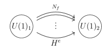
Figure 3: The quiver diagram of two Abelian vertices with $N_{f}$ flavors.

Each edge corresponds to the bi-fundamental matters. So we have $N_{f}$ kinds of the matters (Higgs fields). For the Abelian theory, this means that the matter has a positive charge under one $U(1)_{1}$ gauge group and a negative charge under the other $U(1)_{2}$. The incidence matrix ${L_{v}}^{e}$ is a $2\times N_{f}$ matrix and represents the charges of the matters by

$$L=\overbrace{\left(\begin{array}[]{rrcr}1&1&\cdots&1\\ -1&-1&\cdots&-1\end{array}\right)}^{N_{f}}.$$ (4.1)

In this model, the BPS vortex equation becomes

$$\begin{split}\mu^{1}&=F^{1}-\frac{g_{1}^{2}}{2}\left(\zeta^{1}-\sum_{e=1}^{N_{f}}H^{e}\bar{H}^{e}\right)\omega=0,\\ \mu^{2}&=F^{2}-\frac{g_{2}^{2}}{2}\left(\zeta^{2}+\sum_{e=1}^{N_{f}}\bar{H}^{e}H^{e}\right)\omega=0,\\ \nu^{e}&=2\partial_{A}\bar{H}^{e}=0,\\ \bar{\nu}^{e}&=2\bar{\partial}_{A}H^{e}=0.\end{split}$$ (4.2)

Let us consider linear combinations of $\mu^{1}$ and $\mu^{2}$

$$\frac{1}{g_{1}^{2}}\mu^{1}+\frac{1}{g_{2}^{2}}\mu^{2} = \frac{1}{g_{1}^{2}}F^{1}+\frac{1}{g_{2}^{2}}F^{2}-\frac{1}{2}\left(\zeta^{1}+\zeta^{2}\right)\omega=0,$$ (4.3)

$$\frac{1}{g_{1}^{2}}\mu^{1}-\frac{1}{g_{2}^{2}}\mu^{2} = \frac{1}{g_{1}^{2}}F^{1}-\frac{1}{g_{2}^{2}}F^{2}-\frac{1}{2}\left(\zeta^{1}-\zeta^{2}-2\sum_{e=1}^{N_{f}}H^{e}\bar{H}^{e}\right)\omega=0.$$ (4.4)

Integrating (4.3) on $\Sigma_{h}$, we find

$$\frac{k^{1}}{g_{1}^{2}}+\frac{k^{2}}{g_{2}^{2}}=\frac{\zeta^{1}+\zeta^{2}}{4\pi}{\cal A}.$$ (4.5)

However this equation can not be satisfied for generic value of $g_{v}$ and $\zeta^{v}$ since the magnetic fluxes $k_{v}$ are integer valued. If $\zeta^{1}+\zeta^{2}=0$, there exist the vacuum ($k^{1}=k^{2}=0$) at least, but no BPS vortices is allowed for the generic couplings. If the gauge couplings of two $U(1)$’s coincide with each other $g_{1}=g_{2}$, there are infinitely many BPS vortices when $\zeta^{1}+\zeta^{2}=0$ and $k^{1}+k^{2}=0$. In this case, $U(1)$ of the difference of the generators in $U(1)_{1}$ and $U(1)_{2}$;

$$A^{\prime}=\frac{1}{2}(A^{1}-A^{2})$$ (4.6)

is isomorphic to a single $U(1)$ theory with $N_{f}$ flavors, and eq. (4.4) is equivalent to the BPS vortex equation of $N_{f}$ flavors with the flux $(k^{1}-k^{2})/2=k^{1}$ and FI parameter $(\zeta^{1}-\zeta^{2})/2=\zeta^{1}$.

On the other hand, integrating (4.4) on $\Sigma_{h}$, we get

$$\frac{\zeta^{1}-\zeta^{2}}{4\pi}{\cal A}-\frac{k^{1}}{g_{1}^{2}}+\frac{k^{2}}{g_{2}^{2}}=\frac{1}{2\pi}\sum_{e=1}^{N_{f}}\int_{\Sigma_{h}}H^{e}\bar{H}^{e}\omega\geq 0.$$ (4.7)

This is a Bradlow bound for the relative charges of the vortex. If $g_{1}=g_{2}$, then we need to set $\zeta^{1}+\zeta^{2}=0$ and $k^{1}+k^{2}=0$ and (4.7) reduces to the Bradlow bound for the Abelian theory with the single $U(1)$

$$\frac{\zeta^{1}{\cal A}}{4\pi}-\frac{k^{1}}{g_{1}^{2}}\geq 0.$$ (4.8)

So there exists an upper bound for the vorticity $k^{1}$ on $\Sigma_{h}$ with the finite area ${\cal A}$.

Applying the formula (3.85), we obtain

$$\left\langle e^{i\beta{\cal I}_{V}(g_{v})}\right\rangle^{g_{0,v}=g_{c,v}}_{k^{1},k^{2}}={\cal N}_{C}^{\prime}\int\frac{d\phi_{0}^{1}}{2\pi}\frac{d\phi_{0}^{2}}{2\pi}\frac{(\det\Omega)^{h}}{\left(-i(\phi_{0}^{1}-\phi_{0}^{2})\right)^{N_{f}\left(k^{1}-k^{2}+\frac{1}{2}\chi_{h}\right)}}e^{-2\pi i\beta\left(\phi_{0}^{1}B^{1}+\phi_{0}^{2}B^{2}\right)},$$ (4.9)

where

$$\begin{split}\det\Omega&=\det\begin{pmatrix}\frac{\beta}{g_{1}^{2}}+\frac{1}{2\pi}\frac{N_{f}}{-i(\phi_{0}^{1}-\phi_{0}^{2})}&-\frac{1}{2\pi}\frac{N_{f}}{-i(\phi_{0}^{1}-\phi_{0}^{2})}\\ -\frac{1}{2\pi}\frac{N_{f}}{-i(\phi_{0}^{1}-\phi_{0}^{2})}&\frac{\beta}{g_{2}^{2}}+\frac{1}{2\pi}\frac{N_{f}}{-i(\phi_{0}^{1}-\phi_{0}^{2})}\end{pmatrix}\\ &=\frac{\beta}{g_{1}^{2}g_{2}^{2}}\left(\beta+\frac{g_{1}^{2}+g_{2}^{2}}{2\pi}\frac{N_{f}}{-i(\phi_{0}^{1}-\phi_{0}^{2})}\right).\end{split}$$ (4.10)

Now changing the variables to

$$\begin{split}\phi_{0}^{c}&\equiv\frac{1}{2}(\phi_{0}^{1}+\phi_{0}^{2}),\\ \hat{\phi}_{0}&\equiv\phi_{0}^{1}-\phi_{0}^{2},\\ \hat{k}&\equiv k^{1}-k^{2},\end{split}$$ (4.11)

we can write

$$\begin{split}\left\langle e^{i\beta{\cal I}_{V}(g_{v})}\right\rangle^{g_{0,v}=g_{c,v}}_{\hat{k}}&={\cal N}_{C}^{\prime}\int\frac{d\phi_{0}^{c}}{2\pi}\frac{d\hat{\phi}_{0}}{2\pi}\frac{\left(\frac{\beta}{g_{1}^{2}g_{2}^{2}}\right)^{h}\left(\beta+\frac{g_{1}^{2}+g_{2}^{2}}{2\pi}\frac{N_{f}}{-i\hat{\phi}_{0}}\right)^{h}}{\left(-i\hat{\phi}_{0}\right)^{N_{f}\left(\hat{k}+\frac{1}{2}\chi_{h}\right)}}e^{-2\pi i\beta\left(2\phi_{0}^{c}B^{c}+\frac{1}{2}\hat{\phi}_{0}\hat{B}\right)}\\ &={\cal N}_{C}^{\prime}\int\frac{d\phi_{0}^{c}}{2\pi}\left(\frac{\beta}{g_{1}^{2}g_{2}^{2}}\right)^{h}e^{-4\pi i\beta\phi_{0}^{c}B^{c}}\int\frac{d\hat{\phi}_{0}}{2\pi}\frac{\left(\beta+\frac{g_{1}^{2}+g_{2}^{2}}{2\pi}\frac{N_{f}}{-i\hat{\phi}_{0}}\right)^{h}}{\left(-i\hat{\phi}_{0}\right)^{N_{f}\left(\hat{k}+\frac{1}{2}\chi_{h}\right)}}e^{-\pi i\beta\hat{\phi}_{0}\hat{B}},\end{split}$$ (4.12)

where

$$\begin{split}B^{c}&\equiv\frac{1}{2}(B^{1}+B^{2})=\frac{1}{2}\left(\frac{\zeta^{1}+\zeta^{2}}{4\pi}{\cal A}-\frac{k^{1}}{g_{1}^{2}}-\frac{k^{2}}{g_{2}^{2}}\right),\\ \hat{B}&\equiv B^{2}-B^{2}=\frac{\zeta^{1}-\zeta^{2}}{4\pi}{\cal A}-\frac{k^{1}}{g_{1}^{2}}+\frac{k^{2}}{g_{2}^{2}}.\end{split}$$ (4.13)

The former integral in (4.12) gives

$${\cal N}_{C}^{\prime}\int\frac{d\phi_{0}^{c}}{2\pi}\left(\frac{\beta}{g_{1}^{2}g_{2}^{2}}\right)^{h}e^{-4\pi i\beta\phi_{0}^{c}B^{c}}=\frac{{\cal N}_{C}^{\prime}}{2\pi}\left(\frac{\beta}{g_{1}^{2}g_{2}^{2}}\right)^{h}\delta(2\beta B^{c}),$$ (4.14)

which gives a constraint $B^{c}=0$ as we found from (4.3).

The latter integral in (4.12);

$$\int\frac{d\hat{\phi}_{0}}{2\pi}\frac{\left(\beta+\frac{g_{1}^{2}+g_{2}^{2}}{2\pi}\frac{N_{f}}{-i\hat{\phi}_{0}}\right)^{h}}{\left(-i\hat{\phi}_{0}\right)^{N_{f}\left(\hat{k}+\frac{1}{2}\chi_{h}\right)}}e^{-\pi i\beta\hat{\phi}_{0}\hat{B}},$$ (4.15)

is nothing but the integral expression for the volume of the vortex moduli space in $U(1)$ gauge theory with $N_{f}$ flavors [13, 15] up to a redefinition of the parameter $\beta$.

To evaluate the integral (4.15), we introduce a small twisted mass. Turning on the twisted mass $\epsilon^{e}$ for $H^{e}$, the supersymmetric transformations are modified; e.g.

$$QH^{e}=\psi^{e},\quad Q\psi^{e}=i\phi^{v}{L(H)_{v}}^{e}-\epsilon^{e}H^{e},$$ (4.16)

where we do not sum the repeated index $e$. This modification by the twisted mass also modifies the cohomological volume operator into

$${\cal I}_{V}^{\epsilon}(g_{v})=\int_{\Sigma_{h}}\left[\phi_{v}\mu^{v}(g_{v})+\frac{i}{2}\sum_{e\in E}\epsilon^{e}H^{e}\bar{H}^{e}-\lambda_{v}\wedge\bar{\lambda}^{v}+\frac{i}{2}\psi_{e}\bar{\psi}^{e}\omega\right].$$ (4.17)

Indeed, we can shift the integral path above the real axis without any divergences from the integral of the matter fields, then the integral contour should be closed on the lower half plane (Fig. 4(a)) if $\hat{B}>0$ or on the upper half plane (Fig. 4(b)) if $\hat{B}<0$.

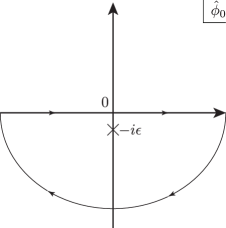
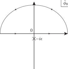
(a) $\hat{B}>0$		(b) $\hat{B}<0$

Figure 4: The integral contours of $\hat{\phi}_{0}$. The pole exists at $\hat{\phi}_{0}=-i\epsilon$. For convergence of the integral, we should choose closed circle on the lower half plane (a) if $\hat{B}>0$ or on the upper half plane (b) if $\hat{B}<0$. The contour (a) includes the pole inside.

The contour includes the pole at $\hat{\phi}_{0}=-i\epsilon$ if $\hat{B}>0$. So the integral gives a non-vanishing value. This is related to the Bradlow bound condition (4.7). Evaluating the integral (4.15), we obtain

$$\begin{split}\int\frac{d\hat{\phi}_{0}}{2\pi}\frac{\left(\beta+\frac{g_{1}^{2}+g_{2}^{2}}{2\pi}\frac{N_{f}}{-i\hat{\phi}_{0}}\right)^{h}e^{-\pi i\beta\hat{\phi}_{0}\hat{B}}}{\left(-i\hat{\phi}_{0}+\epsilon\right)^{N_{f}\left(\hat{k}+\frac{1}{2}\chi_{h}\right)}}&=\sum_{l=0}^{h}\binom{h}{l}\beta^{l}\left(\frac{g_{1}^{2}+g_{2}^{2}}{2\pi}N_{f}\right)^{h-l}\\ &\qquad\qquad\times\int\frac{d\hat{\phi}_{0}}{2\pi}\frac{e^{-\pi i\beta\hat{\phi}_{0}\hat{B}}}{\left(-i\hat{\phi}_{0}+\epsilon\right)^{N_{f}\left(\hat{k}+\frac{1}{2}\chi_{h}\right)+h-l}}\\ &=\beta^{d}\sum_{l=0}^{h}\binom{h}{l}\left(\frac{g_{1}^{2}+g_{2}^{2}}{2\pi}N_{f}\right)^{h-l}\frac{(2\pi\hat{B})^{d-l}e^{-\epsilon\pi\beta\hat{B}}}{(d-l)!},\end{split}$$ (4.18)

where $d\equiv\hat{k}N_{f}+(N_{f}-1)(1-h)$. So we find, in the $\epsilon\to 0$ limit, the volume of the moduli space is proportional to

$$\beta^{d}\sum_{l=0}^{h}\binom{h}{l}\left(\frac{g_{1}^{2}+g_{2}^{2}}{2\pi}N_{f}\right)^{h-l}\frac{(2\pi\hat{B})^{d-l}}{(d-l)!}$$ (4.19)

This is the volume of the moduli space of the Abelian vortex with $N_{f}$ flavor on $\Sigma_{h}$. The dimension of the moduli space is expressed in the power of $\beta$, i.e. $d=\hat{k}N_{f}+(N_{f}-1)(1-h)$.

On the other hand, the integral vanish if $\hat{B}<0$ since the pole at $\hat{\phi}_{0}=0$ is not enclosed inside the contour. This means that there is no BPS vortex solution for $\hat{B}<0$.

To summarize, the volume of the moduli space of the quiver vortex does not vanish if and only if the condition;

$$B_{c}=0\quad\text{and}\quad\hat{B}>0,$$ (4.20)

are satisfied, and takes a value of (4.18). The quiver vortex could exist on $\Sigma_{h}$ with charges which satisfy the condition (4.20).

4.2 Non-compact moduli space

We now consider a model with two vertices, i.e. $G=U(1)_{1}\times U(1)_{2}$ quiver gauge theory. In contrast with the prior model, we have only two matters with opposite charges. Two edge arrows makes a loop between two vertices. The quiver diagram is depicted in Fig. 5.

Figure 5: The quiver diagram of two Abelian vertices with a loop.

The incidence matrix is given by

$$L=\left(\begin{array}[]{rr}1&-1\\ -1&1\end{array}\right)$$ (4.21)

The associated BPS equations are given by

$$\begin{split}\mu^{1}&=F^{1}-\frac{g_{1}^{2}}{2}\left(\zeta^{1}-H^{1}\bar{H}^{1}+\bar{H}^{2}H^{2}\right)\omega=0,\\ \mu^{2}&=F^{2}-\frac{g_{2}^{2}}{2}\left(\zeta^{2}+\bar{H}^{1}H^{1}-H^{2}\bar{H}^{2}\right)\omega=0,\\ \nu^{e}&=2\partial_{A}\bar{H}^{e}=0,\\ \bar{\nu}^{e}&=2\bar{\partial}_{A}H^{e}=0.\end{split}$$ (4.22)

Similar to the prior model, we can consider sum and difference of $\mu^{1}$ and $\mu^{2}$;

$$\frac{1}{g_{1}^{2}}\mu^{1}+\frac{1}{g_{2}^{2}}\mu^{2} = \frac{1}{g_{1}^{2}}F^{1}+\frac{1}{g_{2}^{2}}F^{2}-\frac{1}{2}\left(\zeta^{1}+\zeta^{2}\right)\omega=0,$$ (4.23)

$$\frac{1}{g_{1}^{2}}\mu^{1}-\frac{1}{g_{2}^{2}}\mu^{2} = \frac{1}{g_{1}^{2}}F^{1}-\frac{1}{g_{2}^{2}}F^{2}-\frac{1}{2}\left(\zeta^{1}-\zeta^{2}-2H^{1}\bar{H}^{1}+2\bar{H}^{2}H^{2}\right)\omega=0.$$ (4.24)

From the sum (4.23), we have

$$B^{c}=\frac{1}{2}(B^{1}+B^{2})=0,$$ (4.25)

as a constraint for the couplings and FI parameters. From the difference (4.24), we obtain

$$\hat{B}=B^{1}-B^{2}=\frac{1}{2\pi}\int_{\Sigma_{h}}H^{1}\bar{H}^{1}\omega-\frac{1}{2\pi}\int_{\Sigma_{h}}H^{2}\bar{H}^{2}\omega.$$ (4.26)

So $\hat{B}$ can take any positive and negative values. Thus the moduli space of this model should be non-compact since there are infinitely many combinations of the vev of $H^{1}$ and $H^{2}$, which give the same difference $\hat{B}$. In particular, if we consider the vacuum ($k^{1}=k^{2}=0$) and assume the covariantly constant equations $\nu^{e}=\bar{\nu}^{e}=0$ have non-trivial and normalizable solutions, the vev of $H^{1}$ and $H^{2}$ is given by the difference of the FI parameters

$$|H^{1}|^{2}-|H^{2}|^{2}=\zeta^{1}-\zeta^{2},$$ (4.27)

which represents a non-compact moduli space (hyperbolic plane).

Applying the integral formula (3.85), we obtain

$$\left\langle e^{i\beta{\cal I}_{V}(g_{v})}\right\rangle^{g_{0,v}=g_{c,v}}_{\hat{k}}=(-1)^{\frac{1}{2}\chi_{h}-\hat{k}}{\cal N}_{C}^{\prime}\left(\frac{\beta}{g_{1}g_{2}}\right)^{2h}\int\frac{d\phi_{0}^{c}}{2\pi}e^{-4\pi i\beta\phi_{0}^{c}B^{c}}\int\frac{d\hat{\phi}_{0}}{2\pi}\frac{e^{-\pi i\beta\hat{\phi}_{0}\hat{B}}}{\left(-i\hat{\phi}_{0}\right)^{\chi_{h}}}.$$ (4.28)

The former integral gives the constraint $B^{c}=0$ as expected, but the integral does not depend on the magnetic flux $\hat{k}$ except for the overall sign. Hence the integral of $\hat{\phi}_{0}$ is highly degenerate and the choice of the contour is not well-defined.

This is because the poles associated with $H^{1}\neq 0$ ($\hat{k}>0$) and $H^{2}\neq 0$ ($\hat{k}<0$) are merged. To avoid the degeneration, we modify the model by introducing twisted masses ($\Omega$-backgrounds) for the matter $H^{1}$ and $H^{2}$. The introduction of the twisted masses changes the supersymmetric transformations to

$$\begin{split}Q\psi^{1}&=i(\phi^{1}-\phi^{2}+i\epsilon^{1})H^{1}=i(\hat{\phi}+i\epsilon^{1})H^{1},\\ Q\psi^{2}&=i(\phi^{2}-\phi^{1}+i\epsilon^{2})H^{2}=i(-\hat{\phi}+i\epsilon^{2})H^{2},\end{split}$$ (4.29)

where $\epsilon^{1}$ and $\epsilon^{2}$ are real and positive parameters. The fixed point equation $Q\psi^{1}=Q\psi^{2}=0$ means that $H^{1}\neq 0$ (or $H^{2}\neq 0$) contributes near the pole at $\hat{\phi}_{0}+i\epsilon^{1}\approx 0$ (or $-\hat{\phi}_{0}+i\epsilon^{2}\approx 0$).

Thus, using the separation of the poles, we can distinguish two branches of the non-compact moduli space, which are $\hat{B}>0$ and $H^{1}\neq 0$, or $\hat{B}<0$ and $H^{2}\neq 0$. Turning on the twisted mass does not admit the mixed branch $H^{1}\neq 0$ and $H^{2}\neq 0$.

The integral formula for the volume is also modified by the twisted mass into

$$\begin{split}\left\langle e^{i\beta{\cal I}_{V}(g_{v})}\right\rangle^{g_{0,v}=g_{c,v}}_{\hat{k}}&={\cal N}_{C}^{\prime}\int\frac{d\phi_{0}^{c}}{2\pi}e^{-4\pi i\beta\phi_{0}^{c}B^{c}}\\ &\qquad\times\int\frac{d\hat{\phi}_{0}}{2\pi}\frac{(\det\Omega)^{h}\,e^{-\pi i\beta\hat{\phi}_{0}\hat{B}}}{\left(-i\hat{\phi}_{0}+\epsilon^{1}\right)^{\hat{k}+\frac{1}{2}\chi_{h}}\left(i\hat{\phi}_{0}+\epsilon^{2}\right)^{-\hat{k}+\frac{1}{2}\chi_{h}}},\end{split}$$ (4.30)

where

$$\begin{split}\det\Omega&=\frac{\beta}{g_{1}^{2}g_{2}^{2}}\left(\beta+\frac{g_{1}^{2}+g_{2}^{2}}{2\pi}\frac{1}{-i\hat{\phi}_{0}+\epsilon^{1}}+\frac{g_{1}^{2}+g_{2}^{2}}{2\pi}\frac{1}{i\hat{\phi}_{0}+\epsilon^{2}}\right)\\ &=\frac{\beta}{g_{1}^{2}g_{2}^{2}}\left(\beta+\frac{g_{1}^{2}+g_{2}^{2}}{2\pi}\frac{\epsilon^{1}+\epsilon^{2}}{\left(-i\hat{\phi}_{0}+\epsilon^{1}\right)\left(i\hat{\phi}_{0}+\epsilon^{2}\right)}\right).\end{split}$$ (4.31)

The former integral gives the constraint $B^{c}=0$ again. If $\hat{B}>0$, we need to choose the contour on the lower half plane. Then we obtain the volume of the moduli space as

$$\left\langle e^{i\beta{\cal I}_{V}(g_{v})}\right\rangle^{g_{0,v}=g_{c,v}}_{\hat{k}}={\cal N}_{C}^{\prime\prime}\beta^{\hat{k}}\frac{1}{(\epsilon^{1}+\epsilon^{2})^{1-h-\hat{k}}}\sum_{l=0}^{h}\binom{h}{l}\left(\frac{g_{1}^{2}+g_{2}^{2}}{2\pi}\right)^{h-l}\frac{(2\pi\hat{B})^{\hat{k}-l}}{(\hat{k}-l)!},$$ (4.32)

and $\hat{k}$ should be positive, where

$${\cal N}_{C}^{\prime\prime}\equiv{\cal N}_{C}^{\prime}\left(\frac{\beta}{g_{1}^{2}g_{2}^{2}}\right)^{h}\int\frac{d\phi_{0}^{c}}{2\pi}e^{-4\pi i\beta\phi_{0}^{c}B^{c}},$$ (4.33)

includes the irrelevant constants and constraint. If $\hat{B}<0$, we need to choose the contour on the upper-half plane and get

$$\left\langle e^{i\beta{\cal I}_{V}(g_{v})}\right\rangle^{g_{0,v}=g_{c,v}}_{\hat{k}}={\cal N}_{C}^{\prime\prime}\beta^{-\hat{k}}\frac{1}{(\epsilon^{1}+\epsilon^{2})^{1-h+\hat{k}}}\sum_{l=0}^{h}\binom{h}{l}\left(\frac{g_{1}^{2}+g_{2}^{2}}{2\pi}\right)^{h-l}\frac{(-2\pi\hat{B})^{-\hat{k}-l}}{(-\hat{k}-l)!},$$ (4.34)

and $\hat{k}$ should be negative.

After regularizing the volume by introducing the twisted masses $\epsilon^{1}$ and $\epsilon^{2}$, we find the volume is proportional to $(\epsilon^{1}+\epsilon^{2})^{h+|\hat{k}|-1}$. So the volume diverges in the limit of $\epsilon^{1}\to 0$ and $\epsilon^{2}\to 0$ if $h=0$ and $\hat{k}=0$. This reflects the fact that the moduli space of the vacuum on $S^{2}$, which is given by a non-trivial and normalizable solution to the covariantly constant equations $\nu^{e}=\bar{\nu}^{e}=0$ and eq. (4.27), is non-compact with unit complex dimension. The regularization causes the separation of the branch of the moduli space. Each branch contributes to the volumes as Abelian BPS vortices of $N_{f}=1$. We can see this results from the equation (4.26) if the moduli space is separated by two branches of $\hat{B}>0$, $\hat{k}>0$ and $H^{1}\neq 0$, or $\hat{B}<0$, $\hat{k}<0$ and $H^{2}\neq 0$

For $h=1$ (torus), the volume of the vacuum moduli space takes a constant value and is independent of $\epsilon^{1}$ and $\epsilon^{2}$. This means that the moduli space shrinks to isolated points. (The dimension of the moduli space also vanishes in this case.) For the higher genus case ($h>1$), the volume of the vacuum moduli space vanishes in the limit of $\epsilon^{1}\to 0$ and $\epsilon^{2}\to 0$. In this case, we expect that there is no solution to the differential equations which determine the moduli space of vacua.

The non-existence of vacuum solution on higer genus Riemann surface is not a strange phenomenon. It has been found already in more familiar models with compact moduli spaces, such as the $U(1)$ gauge theory with $N_{f}$ flavors of charged Higgs scalars, by means of cohomologies and divisors [20], and also by means of localization [13]. In the simplest solution ($g_{1}=g_{2}$) of the constraint (4.25), the model is equivalent to a single $U(1)$ gauge theory with two opposite charge scalar fields as given in (4.26). A similar model for compact moduli space is the $U(1)$ gauge theory with two same charge scalar fields, whose moduli space has been found to have similar features [20, 13] : vacuum sector ($k=0$) does not exist for higher genus case ($h>1$), and the moduli space has zero dimension for $h=1$, and unit complex dimension for $h=0$.

4.3 Three Abelian vertices

Non-unidirectional chain

We next consider a quiver diagram with three Abelian vertices. The first example is two matter fields (edges) between three vertices. Orientations of the edges are from the second to the first and from the second to the third; i.e. the two arrows are emitted from the second vertex and oriented in opposite directions to each other. The quiver diagram is depicted in Fig. 6.

Figure 6: The quiver diagram of three Abelian vertices of the non-unidirectional chain.

The incidence matrix is given by

$$L=\left(\begin{array}[]{rr}-1&0\\ 1&1\\ 0&-1\end{array}\right),$$ (4.35)

and the BPS equations are

$$\begin{split}\mu^{1}&=F^{1}-\frac{g_{1}^{2}}{2}\left(\zeta^{1}+\bar{H}^{1}H^{1}\right)\omega=0,\\ \mu^{2}&=F^{2}-\frac{g_{2}^{2}}{2}\left(\zeta^{2}-H^{1}\bar{H}^{1}-H^{2}\bar{H}^{2}\right)\omega=0,\\ \mu^{3}&=F^{3}-\frac{g_{3}^{2}}{2}\left(\zeta^{3}+\bar{H}^{2}H^{2}\right)\omega=0,\\ \nu^{e}&=2\partial_{A}\bar{H}^{e}=0,\\ \bar{\nu}^{e}&=2\bar{\partial}_{A}H^{e}=0.\end{split}$$ (4.36)

Integrating $\mu^{v}$ on $\Sigma_{h}$, we find a constraint and the Bradlow bounds

$$\begin{split}&B^{1}+B^{2}+B^{3}=0,\\ &B^{1}\leq 0,\quad B^{2}\geq 0,\quad B^{3}\leq 0.\end{split}$$ (4.37)

The volume of the moduli space is expressed by an integral over $\phi_{0}^{1}$, $\phi_{0}^{2}$ and $\phi_{0}^{3}$

$$\left\langle e^{i\beta{\cal I}^{\epsilon}_{V}(g_{v})}\right\rangle^{g_{0,v}=g_{c,v}}_{k^{1},k^{2},k^{3}}={\cal N}_{C}^{\prime}\int\frac{d\phi_{0}^{1}}{2\pi}\frac{d\phi_{0}^{2}}{2\pi}\frac{d\phi_{0}^{3}}{2\pi}J_{\epsilon}(\phi_{0}^{1},\phi_{0}^{2},\phi_{0}^{3}),$$ (4.38)

where the integrand $J_{\epsilon}(\phi_{0}^{1},\phi_{0}^{2},\phi_{0}^{3})$ is a rational function of $\phi_{0}^{1}$, $\phi_{0}^{2}$ and $\phi_{0}^{3}$ with poles. Introducing notations

$$\phi_{0}^{vv^{\prime}}\equiv\phi_{0}^{v}-\phi_{0}^{v^{\prime}},\quad k^{vv^{\prime}}\equiv k^{v}-k^{v^{\prime}},$$ (4.39)

the integrand is given by

$$J_{\epsilon}(\phi_{0}^{1},\phi_{0}^{2},\phi_{0}^{3})\equiv\frac{(\det\Omega)^{h}\,e^{-2\pi i\beta\left(\phi_{0}^{1}B^{1}+\phi_{0}^{2}B^{2}+\phi_{0}^{3}B^{3}\right)}}{\left(-i\phi_{0}^{21}+\epsilon^{1}\right)^{k^{21}+\frac{1}{2}\chi_{h}}\left(-i\phi_{0}^{23}+\epsilon^{2}\right)^{k^{23}+\frac{1}{2}\chi_{h}}},$$ (4.40)

for this model after turning on the twisted masses $\epsilon^{1}$ and $\epsilon^{2}$ for each edge, where

$$\det\Omega=\frac{\beta}{g_{1}^{2}g_{2}^{2}g_{3}^{2}}\Bigg{(}\beta^{2}+\frac{\beta}{2\pi}\left(\frac{g_{1}^{2}+g_{2}^{2}}{-i\phi_{0}^{21}+\epsilon^{1}}+\frac{g_{2}^{2}+g_{3}^{2}}{-i\phi_{0}^{23}+\epsilon^{2}}\right)\\ +\frac{1}{(2\pi)^{2}}\frac{g_{1}^{2}g_{2}^{2}+g_{2}^{2}g_{3}^{2}+g_{3}^{2}g_{1}^{2}}{\left(-i\phi_{0}^{21}+\epsilon^{1}\right)\left(-i\phi_{0}^{23}+\epsilon^{2}\right)}\Bigg{)}.$$ (4.41)

Integrating $\phi_{0}^{3}$ and $\phi_{0}^{1}$ first, we obtain

$$\left\langle e^{i\beta{\cal I}^{\epsilon}_{V}(g_{v})}\right\rangle^{g_{0,v}=g_{c,v}}_{k^{1},k^{2},k^{3}}={\cal N}_{C}^{\prime}\int\frac{d\phi_{0}^{2}}{2\pi}\operatorname{Res}_{\phi_{0}^{1}=\phi_{0}^{2}+i\epsilon_{1}}\operatorname{Res}_{\phi_{0}^{3}=\phi_{0}^{2}+i\epsilon_{2}}J_{\epsilon}(\phi_{0}^{1},\phi_{0}^{2},\phi_{0}^{3}),$$ (4.42)

and the condition $B^{1}<0$ and $B^{3}<0$ (and $k^{21}+\frac{1}{2}\chi_{h}>0$ and $k^{23}+\frac{1}{2}\chi_{h}>0$) is needed to contain poles inside the contour and get non-vanishing value. The final integral depends only on $\phi_{0}^{2}$ such as $e^{-2\pi i\beta\phi_{0}^{2}(B^{1}+B^{2}+B^{3})}$, which reduces to the constraint $B^{1}+B^{2}+B^{3}=0$ as expected. (So we also have $B^{2}>0$.)

More concretely, if we consider the case on the sphere ($h=0$), we find

$$\left\langle e^{i\beta{\cal I}^{\epsilon}_{V}(g_{v})}\right\rangle^{g_{0,v}=g_{c,v}}_{k^{1},k^{2},k^{3}}={\cal N}_{C}^{\prime}\int\frac{d\phi_{0}^{2}}{2\pi}e^{-2\pi i\beta\phi_{0}^{2}(B^{1}+B^{2}+B^{3})}\,\frac{(-2\pi B^{1})^{k^{21}}}{k^{21}!}\frac{(-2\pi B^{3})^{k^{23}}}{k^{23}!}e^{-2\pi\beta(\epsilon^{1}B^{1}+\epsilon^{2}B^{2})},$$ (4.43)

which is finite in the limit of $\epsilon^{e}\to 0$ and proportional to a product of two volumes of the moduli space of ani-vortices with $N_{f}=1$.

For higher genus case $h\geq 0$, we can also perform the integral in the similar way by expanding $(\det\Omega)^{h}$.

Unidirectional chain

Next we consider a quiver chain with three vertices and oriented (unidirectional) arrows. The quiver diagram is depicted in Fig. 7.

Figure 7: The quiver diagram of three Abelian vertices of the unidirectional chain (oriented arrows).

The incidence matrix and associated BPS vortex equations are given by

$$L=\left(\begin{array}[]{rr}1&0\\ -1&1\\ 0&-1\end{array}\right),$$ (4.44)

and

$$\begin{split}\mu^{1}&=F^{1}-\frac{g_{1}^{2}}{2}\left(\zeta^{1}-H^{1}\bar{H}^{1}\right)\omega=0,\\ \mu^{2}&=F^{2}-\frac{g_{2}^{2}}{2}\left(\zeta^{2}+\bar{H}^{1}H^{1}-H^{2}\bar{H}^{2}\right)\omega=0,\\ \mu^{3}&=F^{3}-\frac{g_{3}^{2}}{2}\left(\zeta^{3}+\bar{H}^{2}H^{2}\right)\omega=0,\\ \nu^{e}&=2\partial_{A}\bar{H}^{e}=0,\\ \bar{\nu}^{e}&=2\bar{\partial}_{A}H^{e}=0.\end{split}$$ (4.45)

Expected constraint and Bradlow bounds from the BPS equations are

$$\begin{split}&B^{1}+B^{2}+B^{3}=0,\\ &B^{1}\geq 0,\quad B^{3}\leq 0.\end{split}$$ (4.46)

The volume of the moduli space is given by

$$\left\langle e^{i\beta{\cal I}^{\epsilon}_{V}(g_{v})}\right\rangle^{g_{0,v}=g_{c,v}}_{k^{1},k^{2},k^{3}}={\cal N}_{C}^{\prime}\int\frac{d\phi_{0}^{2}}{2\pi}\operatorname{Res}_{\phi_{0}^{1}=\phi_{0}^{2}-i\epsilon_{1}}\operatorname{Res}_{\phi_{0}^{3}=\phi_{0}^{2}+i\epsilon_{2}}J_{\epsilon}(\phi_{0}^{1},\phi_{0}^{2},\phi_{0}^{3}),$$ (4.47)

where

$$J_{\epsilon}(\phi_{0}^{1},\phi_{0}^{2},\phi_{0}^{3})\equiv\frac{(\det\Omega)^{h}\,e^{-2\pi i\beta\left(\phi_{0}^{1}B^{1}+\phi_{0}^{2}B^{2}+\phi_{0}^{3}B^{3}\right)}}{\left(-i\phi_{0}^{12}+\epsilon^{1}\right)^{k^{12}+\frac{1}{2}\chi_{h}}\left(-i\phi_{0}^{23}+\epsilon^{2}\right)^{k^{23}+\frac{1}{2}\chi_{h}}},$$ (4.48)

and

$$\det\Omega=\frac{\beta}{g_{1}^{2}g_{2}^{2}g_{3}^{2}}\Bigg{(}\beta^{2}+\frac{\beta}{2\pi}\left(\frac{g_{1}^{2}+g_{2}^{2}}{-i\phi_{0}^{12}+\epsilon^{1}}+\frac{g_{2}^{2}+g_{3}^{2}}{-i\phi_{0}^{23}+\epsilon^{2}}\right)\\ +\frac{1}{(2\pi)^{2}}\frac{g_{1}^{2}g_{2}^{2}+g_{2}^{2}g_{3}^{2}+g_{3}^{2}g_{1}^{2}}{\left(-i\phi_{0}^{12}+\epsilon^{1}\right)\left(-i\phi_{0}^{23}+\epsilon^{2}\right)}\Bigg{)}.$$ (4.49)

Only the difference from the previous case, we obtain the bounds and constraint as $B^{1}>0$, $B^{3}<0$ and $B^{1}+B^{2}+B^{3}=0$. For the sphere ($h=0$), we also find the volume is proportional to a product of two finite moduli space of vortex and anti-vortex as

$$\frac{(2\pi B^{1})^{k^{12}}}{k^{12}!}\frac{(-2\pi B^{3})^{k^{23}}}{k^{23}!}.$$ (4.50)

This means that total moduli space is compact and determined by the vortex from $\mu^{1}=0$ and anti-vortex from $\mu^{3}=0$ with $N_{f}=1$. As a result, the moduli space determined from $\mu^{2}=0$ still remains finite.

Non-unidirectional closed loop

There are arrows (edges) between the vertices, but two arrows are emitted from the first vertex $U(1)_{1}$ and one arrow is started from $U(1)_{2}$ and ended at $U(1)_{3}$. So there is a loop without one way (unidirectional) arrows. We depicted the quiver diagram in Fig. 8.

Figure 8: The quiver diagram of three Abelian vertices with a non-unidirectional loop.

The incidence matrix is given by

$$L=\left(\begin{array}[]{rrr}1&0&1\\ -1&1&0\\ 0&-1&-1\end{array}\right).$$ (4.51)

The BPS vortex equations are

$$\begin{split}\mu^{1}&=F^{1}-\frac{g_{1}^{2}}{2}\left(\zeta^{1}-H^{1}\bar{H}^{1}-H^{3}\bar{H}^{3}\right)\omega=0,\\ \mu^{2}&=F^{2}-\frac{g_{2}^{2}}{2}\left(\zeta^{2}-H^{2}\bar{H}^{2}+\bar{H}^{1}H^{1}\right)\omega=0,\\ \mu^{3}&=F^{3}-\frac{g_{3}^{2}}{2}\left(\zeta^{3}+\bar{H}^{3}H^{3}+\bar{H}^{2}H^{2}\right)\omega=0,\\ \nu^{e}&=2\partial_{A}\bar{H}^{e}=0,\\ \bar{\nu}^{e}&=2\bar{\partial}_{A}H^{e}=0.\end{split}$$ (4.52)

Integrating $\mu^{v}$ on $\Sigma_{h}$, we get a constraint and bounds

$$\begin{split}&B^{1}+B^{2}+B^{3}=0,\\ &B^{1}\geq 0,\quad B^{3}\leq 0,\\ &B^{1}-B^{3}\geq 0.\end{split}$$ (4.53)

The integral formula of the volume is given by

$$\left\langle e^{i\beta{\cal I}^{\epsilon}_{V}(g_{v})}\right\rangle^{g_{0,v}=g_{c,v}}_{k^{1},k^{2},k^{3}}={\cal N}_{C}^{\prime}\int\frac{d\phi_{0}^{1}}{2\pi}\frac{d\phi_{0}^{2}}{2\pi}\frac{d\phi_{0}^{3}}{2\pi}J_{\epsilon}(\phi_{0}^{1},\phi_{0}^{2},\phi_{0}^{3}),$$ (4.54)

where

$$\begin{split}J_{\epsilon}(\phi_{0}^{1},\phi_{0}^{2},\phi_{0}^{3})&\equiv\frac{(\det\Omega)^{h}\,e^{-2\pi i\beta\left(\phi_{0}^{1}B^{1}+\phi_{0}^{2}B^{2}+\phi_{0}^{3}B^{3}\right)}}{\left(-i\phi_{0}^{12}+\epsilon^{1}\right)^{k^{12}+\frac{1}{2}\chi_{h}}\left(-i\phi_{0}^{23}+\epsilon^{2}\right)^{k^{23}+\frac{1}{2}\chi_{h}}\left(-i\phi_{0}^{13}+\epsilon^{3}\right)^{k^{13}+\frac{1}{2}\chi_{h}}},\\ \phi_{0}^{vv^{\prime}}&\equiv\phi_{0}^{v}-\phi_{0}^{v^{\prime}},\\ k^{vv^{\prime}}&\equiv k^{v}-k^{v^{\prime}},\end{split}$$ (4.55)

and

$$\det\Omega=\frac{\beta}{g_{1}^{2}g_{2}^{2}g_{3}^{2}}\Bigg{(}\beta^{2}+\frac{\beta}{2\pi}\left(\frac{g_{1}^{2}+g_{2}^{2}}{-i\phi_{0}^{12}+\epsilon^{1}}+\frac{g_{2}^{2}+g_{3}^{2}}{-i\phi_{0}^{23}+\epsilon^{2}}+\frac{g_{1}^{2}+g_{3}^{2}}{-i\phi_{0}^{13}+\epsilon^{3}}\right)\\ +\frac{g_{1}^{2}g_{2}^{2}+g_{2}^{2}g_{3}^{2}+g_{3}^{2}g_{1}^{2}}{(2\pi)^{2}}\frac{-2i\phi_{0}^{13}+\epsilon^{1}+\epsilon^{2}+\epsilon^{3}}{\left(-i\phi_{0}^{12}+\epsilon^{1}\right)\left(-i\phi_{0}^{23}+\epsilon^{2}\right)\left(-i\phi_{0}^{13}+\epsilon^{3}\right)}\Bigg{)}.$$ (4.56)

Integrating $\phi_{0}^{1}$ and $\phi_{0}^{3}$ of (4.54) first in turn, we obtain

$$\begin{split}\left\langle e^{i\beta{\cal I}^{\epsilon}_{V}(g_{v})}\right\rangle^{g_{0,v}=g_{c,v}}_{k^{1},k^{2},k^{3}}&={\cal N}_{C}^{\prime}\int\frac{d\phi_{0}^{2}}{2\pi}\Big{[}\operatorname{Res}_{\phi^{1}_{0}=\phi_{0}^{2}-i\epsilon^{1}}\operatorname{Res}_{\phi^{3}_{0}=\phi_{0}^{2}+i\epsilon^{2}}\\ &\qquad\qquad\qquad+\operatorname{Res}_{\phi^{1}_{0}=\phi_{0}^{2}-i(\epsilon^{2}-\epsilon^{3})}\operatorname{Res}_{\phi^{3}_{0}=\phi_{0}^{2}+i\epsilon^{2}}\\ &\qquad\qquad\qquad\quad+\operatorname{Res}_{\phi^{1}_{0}=\phi_{0}^{2}-i\epsilon^{1}}\operatorname{Res}_{\phi^{3}_{0}=\phi_{0}^{1}+i\epsilon^{3}}\\ &\qquad\qquad\qquad\qquad+\operatorname{Res}_{\phi^{1}_{0}=\phi_{0}^{2}-i(\epsilon^{2}-\epsilon^{3})}\operatorname{Res}_{\phi^{3}_{0}=\phi_{0}^{1}+i\epsilon^{3}}\Big{]}J_{\epsilon}(\phi_{0}^{1},\phi_{0}^{2},\phi_{0}^{3}).\end{split}$$ (4.57)

To pick up the residues of the poles inside the contour and obtain a non-vanishing volume, we need to assume that $B^{1}>0$ and $B^{3}<0$, which agrees with the Bradlow bound. In the final integral of $\phi_{0}^{2}$, the integrand depends only on $\phi_{0}^{2}$ through the factor $e^{-2\pi i\beta\phi_{0}^{2}(B^{1}+B^{2}+B^{3})}$. So the integral by $\phi_{0}^{2}$ gives the constraint $B^{1}+B^{2}+B^{3}=0$.

For simplicity, let us consider a vacuum on the sphere ($k^{v}=0$ and $h=0$). In this case, we can ignore the contribution from $\det\Omega$. The volume of the moduli space is proportional to

$$\frac{e^{-\beta(\epsilon^{1}\zeta^{1}+(\epsilon^{1}-\epsilon^{3})\zeta^{3}){\cal A}/2}}{\epsilon^{1}+\epsilon^{2}-\epsilon^{3}}\left(1-e^{\beta(\epsilon^{1}+\epsilon^{2}-\epsilon^{3})\zeta^{3}{\cal A}/2}\right),$$ (4.58)

which takes a finite value $-\beta\zeta^{3}{\cal A}/2$ in the limit of $\epsilon^{e}\to 0$. So we can see the moduli space of vacua is compact at least.

Unidirectional closed loop

Let us consider one more case of the three vertices. In contrast with the previous case, all arrows are aligned in one direction (unidirectional) on the loop. The quiver diagram is depicted in Fig. 9.

Figure 9: The quiver diagram of three Abelian vertices with a unidirectional loop.

The incidence matrix is given by

$$L=\left(\begin{array}[]{rrr}1&0&-1\\ -1&1&0\\ 0&-1&1\end{array}\right).$$ (4.59)

The associated BPS vortex equations are

$$\begin{split}\mu^{1}&=F^{1}-\frac{g_{1}^{2}}{2}\left(\zeta^{1}-H^{1}\bar{H}^{1}+\bar{H}^{3}H^{3}\right)\omega=0,\\ \mu^{2}&=F^{2}-\frac{g_{2}^{2}}{2}\left(\zeta^{2}-H^{2}\bar{H}^{2}+\bar{H}^{1}H^{1}\right)\omega=0,\\ \mu^{3}&=F^{3}-\frac{g_{3}^{2}}{2}\left(\zeta^{3}-H^{3}\bar{H}^{3}+\bar{H}^{2}H^{2}\right)\omega=0,\\ \nu^{e}&=2\partial_{A}\bar{H}^{e}=0,\\ \bar{\nu}^{e}&=2\bar{\partial}_{A}H^{e}=0.\end{split}$$ (4.60)

Each $\mu^{v}$ contains both of positive and negative charge matters. So the moduli space of vacua at least is non-compact.

The volume of the moduli space is given by the following integral

$$\left\langle e^{i\beta{\cal I}^{\epsilon}_{V}(g_{v})}\right\rangle^{g_{0,v}=g_{c,v}}_{k^{1},k^{2},k^{3}}={\cal N}_{C}^{\prime}\int\frac{d\phi_{0}^{1}}{2\pi}\frac{d\phi_{0}^{2}}{2\pi}\frac{d\phi_{0}^{3}}{2\pi}J_{\epsilon}(\phi_{0}^{1},\phi_{0}^{2},\phi_{0}^{3}),$$ (4.61)

where

$$J_{\epsilon}(\phi_{0}^{1},\phi_{0}^{2},\phi_{0}^{3})\equiv\frac{(\det\Omega)^{h}\,e^{-2\pi i\beta\left(\phi_{0}^{1}B^{1}+\phi_{0}^{2}B^{2}+\phi_{0}^{3}B^{3}\right)}}{\left(-i\phi_{0}^{12}+\epsilon^{1}\right)^{k^{12}+\frac{1}{2}\chi_{h}}\left(-i\phi_{0}^{23}+\epsilon^{2}\right)^{k^{23}+\frac{1}{2}\chi_{h}}\left(-i\phi_{0}^{31}+\epsilon^{3}\right)^{k^{31}+\frac{1}{2}\chi_{h}}},$$ (4.62)

and

$$\det\Omega=\frac{\beta}{g_{1}^{2}g_{2}^{2}g_{3}^{2}}\Bigg{(}\beta^{2}+\frac{\beta}{2\pi}\left(\frac{g_{1}^{2}+g_{2}^{2}}{-i\phi_{0}^{12}+\epsilon^{1}}+\frac{g_{2}^{2}+g_{3}^{2}}{-i\phi_{0}^{23}+\epsilon^{2}}+\frac{g_{3}^{2}+g_{1}^{2}}{-i\phi_{0}^{31}+\epsilon^{3}}\right)\\ +\frac{g_{1}^{2}g_{2}^{2}+g_{2}^{2}g_{3}^{2}+g_{3}^{2}g_{1}^{2}}{(2\pi)^{2}}\frac{\epsilon^{1}+\epsilon^{2}+\epsilon^{3}}{\left(-i\phi_{0}^{12}+\epsilon^{1}\right)\left(-i\phi_{0}^{23}+\epsilon^{2}\right)\left(-i\phi_{0}^{31}+\epsilon^{3}\right)}\Bigg{)}.$$ (4.63)

Thus the volume of the moduli space is given by residues of $J_{\epsilon}$

$$\left\langle e^{i\beta{\cal I}^{\epsilon}_{V}(g_{v})}\right\rangle^{g_{0,v}=g_{c,v}}_{k^{1},k^{2},k^{3}}\\ =\begin{cases}{\cal N}_{C}^{\prime}\int\frac{d\phi_{0}^{1}}{2\pi}\operatorname{Res}_{\phi^{2}_{0}=\phi_{0}^{1}-i(\epsilon^{2}+\epsilon^{3})}\operatorname{Res}_{\phi^{3}_{0}=\phi_{0}^{1}-i\epsilon^{3}}J_{\epsilon}(\phi_{0}^{1},\phi_{0}^{2},\phi_{0}^{3})&\text{if }B^{3}>0\text{ and }B^{2}>0\\ {\cal N}_{C}^{\prime}\int\frac{d\phi_{0}^{1}}{2\pi}\operatorname{Res}_{\phi^{2}_{0}=\phi_{0}^{1}+i\epsilon^{1}}\operatorname{Res}_{\phi^{3}_{0}=\phi_{0}^{1}-i\epsilon^{3}}J_{\epsilon}(\phi_{0}^{1},\phi_{0}^{2},\phi_{0}^{3})&\text{if }B^{3}>0\text{ and }B^{2}<0\\ {\cal N}_{C}^{\prime}\int\frac{d\phi_{0}^{1}}{2\pi}\operatorname{Res}_{\phi^{2}_{0}=\phi_{0}^{1}-i(\epsilon^{2}+\epsilon^{3})}\operatorname{Res}_{\phi^{3}_{0}=\phi_{0}^{2}+i\epsilon^{2}}J_{\epsilon}(\phi_{0}^{1},\phi_{0}^{2},\phi_{0}^{3})&\text{if }B^{3}<0\text{ and }B^{2}>0\\ {\cal N}_{C}^{\prime}\int\frac{d\phi_{0}^{1}}{2\pi}\operatorname{Res}_{\phi^{2}_{0}=\phi_{0}^{1}+i\epsilon^{1}}\operatorname{Res}_{\phi^{3}_{0}=\phi_{0}^{2}+i\epsilon^{2}}J_{\epsilon}(\phi_{0}^{1},\phi_{0}^{2},\phi_{0}^{3})&\text{if }B^{3}<0\text{ and }B^{2}<0.\end{cases}$$ (4.64)

In particular, if we consider the vacuum on the sphere ($k^{v}=0$ and $h=0$), we obtain

$$\left\langle e^{i\beta{\cal I}^{\epsilon}_{V}(g_{v})}\right\rangle^{g_{0,v}=g_{c,v}}_{k^{1},k^{2},k^{3}}=-{\cal N}_{C}^{\prime}\int\frac{d\phi_{0}^{1}}{2\pi}e^{-i\beta\phi_{0}^{1}(\zeta^{1}+\zeta^{2}+\zeta^{3}){\cal A}/2}\frac{e^{-\beta\left((\epsilon^{2}+\epsilon^{3})\zeta^{2}+\epsilon^{3}\zeta^{3}\right){\cal A}/2}}{\epsilon^{1}+\epsilon^{2}+\epsilon^{3}},$$ (4.65)

if $B^{3}>0$ and $B^{2}>0$. Including all other cases, each volume is proportional to $1/(\epsilon^{1}+\epsilon^{2}+\epsilon^{3})$ and diverges in the limit of $\epsilon^{e}\to 0$. This means that the volume of the moduli space of vacua is non-compact.

Finally, we would like to comment on an interesting fact. Each residues in (4.64) diverges in the limit of $\epsilon^{e}\to 0$ as mentioned, but the total sum of the volumes of the vacua for each region becomes

$${\cal N}_{C}^{\prime}\int\frac{d\phi_{0}^{1}}{2\pi}e^{-i\beta\phi_{0}^{1}(\zeta^{1}+\zeta^{2}+\zeta^{3}){\cal A}/2}\frac{e^{\beta(\epsilon^{1}\zeta^{2}-\epsilon^{3}\zeta^{3}){\cal A}/2}\left(e^{\beta(\epsilon^{1}+\epsilon^{2}+\epsilon^{3})\zeta^{3}{\cal A}/2}-1\right)}{\epsilon^{1}+\epsilon^{2}+\epsilon^{3}},$$ (4.66)

which is finite in the limit of $\epsilon^{e}\to 0$. This is similar to the previous case of the compact moduli space. The contributions of the divergence from each region seem to be complementary to each other.

5 Application to Vortex in Gauged Non-linear Sigma Model

In this section, we would like to consider vortices in gauged non-linear sigma model on a generic Riemann surface $\Sigma_{h}$ with a genus $h$. If we assume that a target space is a Kähler manifold $X$, the (anti-)BPS vortex equation is defined by

$$\begin{split}\mu&=F-\frac{g^{2}}{2}\left(\zeta+||Z||^{2}\right)=0,\\ \nu^{i}&=2\partial_{A}\bar{Z}^{i}=0,\\ \bar{\nu}^{i}&=2\bar{\partial}_{A}Z^{i}=0,\end{split}$$ (5.1)

where $Z^{i}$ are the (inhomogeneous) coordinates of $X$ and $||Z||^{2}$ is a positive definite mapping function from $X$ to $\mathbb{R}$ (moment map), which is invariant under a part of $U(1)$ isometries of $X$. The $U(1)$ gauge symmetry is regarded as a gauging of the $U(1)$ isometry of $X$, under which the moment map $||Z||^{2}$ is invariant. For later convenience, we here consider the anti-BPS equation; i.e. the flux $k=\frac{1}{2\pi}\int_{\Sigma_{h}}F$ and FI parameter $\zeta$ should be negative. We will consider only the case of $X=\mathbb{C}P^{N}$ as an example in the following.

According to [21], the above vortex system in gauged non-linear sigma model can be obtained in a strong coupling limit of a certain gauged linear sigma model (GLSM). The GLSM contains two $U(1)$ gauge groups and two kinds of matter (Higgs) fields, whose total number is $N+1$ ($N+1$ arrows in total). $n$ of the matter fields are charged with respect to both $U(1)$ and denoted as $H^{e}$ ($e=1,2,\ldots,n$). The other $N-n+1$ matter fields have positive charges only on one $U(1)$ and are denoted as $H^{e^{\prime}}$ ($e^{\prime}=n+1,n+2,\ldots,N+1$). We call this model as a parent GLSM following [21].

The parent GLSM is expressed in terms of the quiver gauge theory. The generic quiver gauge theory contains only the bi-fundamental matters (charged under two $U(1)$ vertices), and no fields in the fundamental representation. However, we can introduce a decoupled vertex, which is defined as a vertex with decoupled gauge fields; i.e. the gauge coupling on that vertex is taken in the weak coupling limit. Since the decoupled vertex $U(N)$ stands for a global $U(N)$ symmetry instead of a local symmetry, a matter associated with an arrow between a $U(N_{c})$ vertex and a decoupled vertex becomes $N$ flavors of fields in the fundamental representation of $U(N_{c})$ (charged fields if $N_{c}=1$). We will denote the decoupled vertex in terms of box vertex.

The quiver diagram of the parent GLSM is depicted in Fig. 10. There is $n$ arrows between two $U(1)$ vertices, which correspond to $H^{e}$. We also have $N-n+1$ arrows from one $U(1)$ to the fixed vertex, which represent the matter fields $H^{e^{\prime}}$.

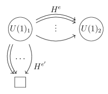
Figure 10: The quiver diagram with two Abelian vertices which is a parent of the gauged non-linear $\sigma$-model. The box stands for a decoupled vertex.

Taking care with the charges (representations) of the matter fields, we can write down the BPS vortex equations for the parent GLSM as

$$\begin{split}\mu^{1}&=F^{1}-\frac{g_{1}^{2}}{2}\left(\zeta^{1}-\sum_{e=1}^{n}H^{e}\bar{H}^{e}-\sum_{e^{\prime}=n+1}^{N+1}H^{e^{\prime}}\bar{H}^{e^{\prime}}\right)\omega=0,\\ \mu^{2}&=F^{2}-\frac{g_{2}^{2}}{2}\left(\zeta^{2}+\sum_{e=1}^{n}\bar{H}^{e}H^{e}\right)\omega=0,\\ \nu^{e}&=2\left(\partial-iA^{1}+iA^{2}\right)\bar{H}^{e}=0,\\ \bar{\nu}^{e}&=2\left(\bar{\partial}+i\bar{A}^{1}-i\bar{A}^{2}\right)H^{e}=0,\\ \nu^{e^{\prime}}&=2\left(\partial-iA^{1}\right)\bar{H}^{e^{\prime}}=0,\\ \bar{\nu}^{e^{\prime}}&=2\left(\bar{\partial}+i\bar{A}^{1}\right)H^{e^{\prime}}=0.\end{split}$$ (5.2)

Integrating $\mu^{v}$ on $\Sigma_{h}$, we can see Bradlow bounds

$$B^{1}\geq 0,\quad B^{2}\leq 0.$$ (5.3)

In addition to the above, if we consider a linear combination $\mu^{1}+\mu^{2}$, then we particularly have

$$B^{1}+B^{2}\geq 0.$$ (5.4)

In contrast with the generic quiver model in the previous section, there is no constraint on $B^{v}$’s, reflecting the existence of the decoupled vertex.

In the parent GLSM, we have two gauge couplings $g_{1}$ and $g_{2}$ associated with two $U(1)$’s. If we take a strong coupling limit of one gauge coupling $g_{1}\to\infty$, the matter fields are captured on a constraint

$$\sum_{e=1}^{n}H^{e}\bar{H}^{e}+\sum_{e^{\prime}=n+1}^{N+1}H^{e^{\prime}}\bar{H}^{e^{\prime}}=\zeta^{1}.$$ (5.5)

Using this constraint and quotient by $U(1)$ gauge symmetry, we can regard $H^{e}$ as a set of the inhomogeneous coordinate of $\mathbb{C}P^{N}$. Thus we expect that

$$\mu^{2}=\nu^{e}=\bar{\nu}^{e}=0\quad(e=1,\ldots,n),$$ (5.6)

express the BPS equation (5.1) of the (anti-)vortex of the gauged non-linear sigma model with the target $\mathbb{C}P^{N}$ in the strong coupling limit $g_{1}\to\infty$.

We are interested in the volume of the moduli space of the vortex in the gauged non-linear sigma model with the target $\mathbb{C}P^{N}$. However we first would like to derive the volume of the moduli space of the parent quiver theory by using the integral formula in the Coulomb branch, since we can obtain the non-linear sigma model in the strong coupling limit.

The incidence matrix of the parent quiver theory is given by

$$\raisebox{-3.87498pt}{$L=\,$}\blockarray{rcrrcr}\BAmulticolumn{3}{r}{\overbrace{\hskip 60.0pt}^{n}}&\BAmulticolumn{3}{c}{\overbrace{\hskip 48.0pt}^{N-n+1}}\\ \block{(rcrrcr)}1\cdots 11\cdots 1\\ -1\cdots-10\cdots 0\\ \ ,$$ (5.7)

The $N-n+1$ right-most columns represent the matters (arrows) from one $U(1)$ vertex to the decoupled vertex and contains only the positive charge $+1$. This point is rather special than the usual incidence matrix of the oriented graph.

Using the generic integral formula for the quiver theory, the volume of the moduli space of the vortices in the parent GLSM is given by

$$\left\langle e^{i\beta{\cal I}^{\epsilon}_{V}(g_{v})}\right\rangle^{g_{0,v}=g_{c,v}}_{k^{1},k^{2}}={\cal N}_{C}^{\prime}\int\frac{d\phi_{0}^{1}}{2\pi}\frac{d\phi_{0}^{2}}{2\pi}J_{\epsilon}(\phi_{0}^{1},\phi_{0}^{2}).$$ (5.8)

Turning on twisted masses $\epsilon$ and $\epsilon^{\prime}$ for $H^{e}$ and $H^{e^{\prime}}$, respectively, the integrand becomes

$$J_{\epsilon}(\phi_{0}^{1},\phi_{0}^{2})=\frac{(\det\Omega_{\epsilon})^{h}\,e^{-2\pi i\beta\left(\phi_{0}^{1}B^{1}+\phi_{0}^{2}B^{2}\right)}}{(-i\phi_{0}^{12}+\epsilon)^{n\left(k^{12}+\frac{1}{2}\chi_{h}\right)}(-i\phi_{0}^{1}+\epsilon^{\prime})^{(N-n+1)\left(k^{1}+\frac{1}{2}\chi_{h}\right)}},$$ (5.9)

where

$$\begin{split}\det\Omega_{\epsilon}&=\frac{1}{g_{1}^{2}g_{2}^{2}}\left(\beta^{2}+\frac{\beta}{2\pi}\left(\frac{n(g_{1}^{2}+g_{2}^{2})}{-i\phi_{0}^{12}+\epsilon}+\frac{(N-n+1)g_{1}^{2}}{-i\phi_{0}^{1}+\epsilon^{\prime}}\right)+\frac{1}{(2\pi)^{2}}\frac{n(N-n+1)g_{1}^{2}g_{2}^{2}}{(-i\phi_{0}^{12}+\epsilon)(-i\phi_{0}^{1}+\epsilon^{\prime})}\right)\\ &=\left(\frac{\beta}{g_{2}^{2}}+\frac{1}{2\pi}\frac{n}{-i\phi_{0}^{12}+\epsilon}\right)\left(\frac{\beta}{g_{1}^{2}}+\frac{\beta}{g_{2}^{2}}+\frac{1}{2\pi}\frac{N-n+1}{-i\phi_{0}^{1}+\epsilon^{\prime}}\right)-\frac{\beta^{2}}{g_{2}^{4}}\,.\end{split}$$ (5.10)

Here we rearranged $\det\Omega_{\epsilon}$ in the final form for later convenience.

We first expand $(\det\Omega_{\epsilon})^{h}$ by using the binomial theorem as

$$\begin{split}(\det\Omega_{\epsilon})^{h}&=\sum_{l=0}^{h}\binom{h}{l}\left(-\frac{\beta^{2}}{g_{2}^{4}}\right)^{l}\left(\frac{\beta}{g_{2}^{2}}+\frac{1}{2\pi}\frac{n}{-i\phi_{0}^{12}+\epsilon}\right)^{h-l}\left(\frac{\beta}{g_{1}^{2}}+\frac{\beta}{g_{2}^{2}}+\frac{1}{2\pi}\frac{N-n+1}{-i\phi_{0}^{1}+\epsilon^{\prime}}\right)^{h-l}\\ &=\sum_{l=0}^{h}\binom{h}{l}\left(-\frac{\beta^{2}}{g_{2}^{4}}\right)^{l}\left\{\sum_{j^{12}=l}^{h}\binom{h-l}{j^{12}-l}\left(\frac{\beta}{g_{2}^{2}}\right)^{j^{12}-l}\left(\frac{1}{2\pi}\frac{n}{-i\phi_{0}^{12}+\epsilon}\right)^{h-j^{12}}\right\}\\ &\qquad\qquad\qquad\quad\times\left\{\sum_{j^{1}=l}^{h}\binom{h-l}{j^{1}-l}\left(\frac{\beta}{g_{1}^{2}}+\frac{\beta}{g_{2}^{2}}\right)^{j^{1}-l}\left(\frac{1}{2\pi}\frac{N-n+1}{-i\phi_{0}^{1}+\epsilon^{\prime}}\right)^{h-j^{1}}\right\}\,.\end{split}$$ (5.11)

Then the integrand $J_{\epsilon}(\phi_{0}^{1},\phi_{0}^{2})$ also can be expanded as follows

$$\begin{split}J_{\epsilon}(\phi_{0}^{1},\phi_{0}^{2})&=\sum_{l=0}^{h}\frac{h!(h-l)!}{(-1)^{l}l!}\left(\frac{\beta}{g_{2}^{2}}\right)^{2l}\\ &\qquad\qquad\times\left\{\sum_{j^{12}=l}^{h}\frac{\left(\frac{n}{2\pi}\right)^{h-j^{12}}\left(\frac{\beta}{g_{2}^{2}}\right)^{j^{12}-l}}{(j^{12}-l)!(h-j^{12})!}\frac{1}{(-i\phi_{0}^{12}+\epsilon)^{d^{12}-j^{12}+1}}\right\}\\ &\qquad\qquad\times\left\{\sum_{j^{1}=l}^{h}\frac{\left(\frac{N-n+1}{2\pi}\right)^{h-j^{1}}\left(\frac{\beta}{g_{1}^{2}}+\frac{\beta}{g_{2}^{2}}\right)^{j^{1}-l}}{(j^{1}-l)!(h-j^{1})!}\frac{1}{(-i\phi_{0}^{1}+\epsilon^{\prime})^{d^{1}-j^{1}+1}}\right\}\\ &\qquad\qquad\times e^{-2\pi i\beta(\phi_{0}^{1}B^{1}+\phi_{0}^{2}B^{2})},\end{split}$$ (5.12)

where we have defined $d^{12}\equiv nk^{12}+(n-1)(1-h)$ and $d^{1}\equiv(N-n+1)k^{1}+(N-n)(1-h)$.

Using this expansion, we can integrate $\phi_{0}^{2}$ and $\phi_{0}^{1}$ in turn. The volume is expressed in terms of the residues for each term

$$\begin{split}\left\langle e^{i\beta{\cal I}^{\epsilon}_{V}(g_{v})}\right\rangle^{g_{0,v}=g_{c,v}}_{k^{1},k^{2}}&={\cal N}_{C}^{\prime}\operatorname{Res}_{\phi_{0}^{1}=-i\epsilon^{\prime}}\operatorname{Res}_{\phi_{0}^{2}=\phi_{0}^{1}+i\epsilon}J_{\epsilon}(\phi_{0}^{1},\phi_{0}^{2})\\ &={\cal N}_{C}^{\prime}\frac{(2\pi\beta)^{d^{12}+d^{1}}}{(2\pi)^{2h}}\sum_{l=0}^{h}\frac{h!(h-l)!}{(-1)^{l}l!}\left(\frac{1}{g_{2}^{2}}\right)^{2l}\\ &\qquad\qquad\times\left\{\sum_{j^{12}=l}^{h}\frac{n^{h-j^{12}}\left(\frac{1}{g_{2}^{2}}\right)^{j^{12}-l}\left(-B^{2}\right)^{d^{12}-j^{12}}}{(j^{12}-l)!(h-j^{12})!(k^{12}-j^{12})!}\right\}\\ &\qquad\qquad\times\left\{\sum_{j^{1}=l}^{h}\frac{(N-n+1)^{h-j^{1}}\left(\frac{1}{g_{1}^{2}}+\frac{1}{g_{2}^{2}}\right)^{j^{1}-l}(B^{1}+B^{2})^{d^{1}-j^{1}}}{(j^{1}-l)!(h-j^{1})!(d^{1}-j^{1})!}\right\}\\ &\qquad\qquad\times e^{-2\pi\epsilon B^{1}-2\pi(\epsilon^{\prime}-\epsilon)B^{2}}.\end{split}$$ (5.13)

We need to require at least

$$d^{12}=nk^{12}+(n-1)(1-h)\geq 0\quad\text{and}\quad d^{1}=(N-n+1)k^{1}+(N-n)(1-h)\geq 0.$$ (5.14)

So we have

$$k^{12}\geq\max\left\{0,\frac{(n-1)(h-1)}{n}\right\}\quad\text{and}\quad k^{1}\geq\max\left\{0,\frac{(N-n)(h-1)}{N-n+1}\right\}.$$ (5.15)

In integrating $\phi_{0}^{2}$, we get a bound

$$B^{2}<0,$$ (5.16)

to include the pole at $\phi_{0}^{2}=\phi_{0}^{1}+i\epsilon$ inside the contour. The integral of $\phi_{0}^{1}$ also gives

$$B^{1}+B^{2}>0,$$ (5.17)

as a consequence of the pole at $\phi_{0}^{1}=-i\epsilon$. These agree with the Bradlow bounds.

The volume is always finite in the limit of $\epsilon\to 0$ and $\epsilon^{\prime}\to 0$ (removing the regularization). Our result in Eq. (5.13) with $\epsilon=\epsilon^{\prime}=0$ gives the moduli space volume of BPS vortices in the $U(1)_{1}\times U(1)_{2}$ GLSM with $n$ bifundamental and $N-n+1$ fundamental scalar fields. When restricted to $N=1$ and $n=1$ (corresponding to $X=\mathbb{C}P^{1}$ case), our GLSM reduces to that studied in [21]. The results precisely agree with each other provided different conventions are appropriately translated. Our field theoretical derivation is based on a scheme that is entirely different from that in [21]. Moreover, our results include the more general cases for generic $N$ and $n$ (corresponding to $X=\mathbb{C}P^{N}$ case with $n$ flavors of charged scalars) and are obtained without any concrete knowledge of the moduli space including the metric.

The dimension of the moduli space is given by the overall power of $\beta$. So we can see the dimension of the total moduli space is $d^{12}+d^{1}$, which is the sum of the dimension of the moduli space of the Abelian vortex with $n$ and $N-n+1$ flavors. And also the volume of the moduli space (5.13) is an almost direct product of each Abelian vortex moduli space with $n$ and $N-n+1$ matters, except for the combinatorial factor and sums.

We found the volume of the vortex moduli space of the parent model. As we explained above, we can expect that the volume of the vortex moduli space of the non-linear sigma model with the target space $\mathbb{C}P^{N}$ can be obtained by the strong coupling limit of $g_{1}\to\infty$.

In this limit, we find

$$B^{1}\to\frac{\zeta^{1}{\cal A}}{4\pi}.$$ (5.18)

Thus we obtain the volume of the vortex moduli space of the $U(1)$ GNLSM with the target space $\mathbb{C}P^{N}$ and with $n$ flavors as

$$\begin{split}\lim_{\begin{subarray}{c}\epsilon,\epsilon^{\prime}\to 0\\ g_{1}\to\infty\end{subarray}}\left\langle e^{i\beta{\cal I}^{\epsilon}_{V}(g_{v})}\right\rangle^{g_{0,v}=g_{c,v}}_{k^{1},k^{2}}&={\cal N}_{C}^{\prime}\frac{(2\pi\beta)^{d^{12}+d^{1}}}{(2\pi)^{2h}}\sum_{l=0}^{h}\frac{h!(h-l)!}{(-1)^{l}l!}\\ &\qquad\qquad\times\left\{\sum_{j^{12}=l}^{h}\frac{n^{h-j^{12}}\left(\frac{1}{g_{2}^{2}}\right)^{j^{12}}\left(-B^{2}\right)^{d^{12}-j^{12}}}{(j^{12}-l)!(h-j^{12})!(k^{12}-j^{12})!}\right\}\\ &\qquad\qquad\times\left\{\sum_{j^{1}=l}^{h}\frac{(N-n+1)^{h-j^{1}}\left(\frac{1}{g_{2}^{2}}\right)^{j^{1}}\left(B^{2}+\frac{\zeta^{1}{\cal A}}{4\pi}\right)^{d^{1}-j^{1}}}{(j^{1}-l)!(h-j^{1})!(d^{1}-j^{1})!}\right\}.\end{split}$$ (5.19)

6 Non-Abelian Generalization

6.1 Action and integral formula

We now generalize the Abelian quiver gauge theory to quiver gauge theory with non-Abelian vertices. There exist $U(N)$ non-Abelian gauge groups on each vertex. So we have quiver gauge theory with a gauge symmetry $G=\prod_{v\in V}U(N_{v})$, where $N_{v}$ is a rank of gauge group on a vertex $v\in V$.

There are also directed arrows (edges) connecting between vertices, which represents matter fields in bi-fundamental representations. If we pick up one edge $e\in E$, the matter field transform as a fundamental representation under the gauge group $U(N_{s(e)})$ at the source of the edge and anti-fundamental representation under $U(N_{t(e)})$ at the target of the edge. So the BPS quiver vortex equations for this non-Abelian theory are given by

$$\mu^{v}=\nu^{e}=\bar{\nu}^{e}=0.$$ (6.1)

Next, we consider an embedding of the above BPS vortex system into a supersymmetric gauge theory. To define the supersymmetric gauge theory, we introduce vector multiplets and chiral multiplets. The vector multiplets exist on each vertex $v$ and contain 0-form scalar fields $\Phi^{v}$, 1-form vector fields $(A^{v},\bar{A}^{v})$, 2-form auxiliary fields $Y^{v}$, and their fermionic super partners $\eta^{v}$, $(\lambda^{v},\bar{\lambda}^{v})$, $\chi^{v}$. All fields are $N_{v}\times N_{v}$ matrices and belong to the adjoint representation.

The supersymmetry transformations of the vector multiplets are given by

$$\begin{array}[]{lcl}Q\Phi^{v}=0,&&\\ Q\bar{\Phi}^{v}=2\eta^{v},&&Q\eta^{v}=\frac{i}{2}[\Phi^{v},\bar{\Phi}^{v}],\\ QA^{v}=\lambda^{v},&&Q\lambda^{v}=-\partial_{A}\Phi^{v},\\ Q\bar{A}^{v}=\bar{\lambda}^{v},&&Q\bar{\lambda}^{v}=-\bar{\partial}_{A}\Phi^{v},\\ QY^{v}=i[\Phi^{v},\chi^{v}],&&Q\chi^{v}=Y^{v},\end{array}$$ (6.2)

where $\partial_{A}\Phi^{v}\equiv\partial\Phi^{v}+i[A^{v},\Phi^{v}]$ and $\bar{\partial}_{A}\Phi^{v}\equiv\bar{\partial}\Phi^{v}+i[\bar{A}^{v},\Phi^{v}]$. We can see $Q^{2}=\delta_{\Phi}$, which is a gauge transformation with respect to a parameter $\Phi^{v}$.

The chiral multiplets correspond to each arrow on the graph. We can devide the chiral multiplets into two sets. One of the sets contains $N_{s(e)}\times N_{t(e)}$ matrix of 0-form bosons and fermions, which we denote by $(H^{e},\psi^{e})$, and $(0,1)$-forms $(\bar{T}^{e},\bar{\rho}^{e})$. For this part of the chiral multiplets, we can define the supersymmetry by

$$\begin{array}[]{lcl}QH^{e}=\psi^{e},&&Q\psi^{e}=i\Phi^{v}\cdot{L(H)_{v}}^{e},\\ Q\bar{T}^{e}=i\Phi^{v}\cdot{L(\bar{\rho})_{v}}^{e},&&Q\bar{\rho}^{e}=\bar{T}^{e},\end{array}$$ (6.3)

where

$$\begin{split}\Phi^{v}\cdot{L(H)_{v}}^{e}&\equiv\Phi^{s(e)}H^{e}-H^{e}\Phi^{t(e)},\\ \Phi^{v}\cdot{L(\bar{\rho})_{v}}^{e}&\equiv\Phi^{s(e)}\bar{\rho}^{e}-\bar{\rho}^{e}\Phi^{t(e)},\end{split}$$ (6.4)

i.e. ${L(H)_{v}}^{e}$ is a non-Abelian generalization of the (covariant) incidence matrix, and $\Phi^{v}$ is acting on the bi-fundamental representation $H^{e}$ in a suitable way. Again we can see $Q^{2}=\delta_{\Phi}$.

Another set of the chiral multiplets is a conjugate of the above. We have $N_{t(e)}\times N_{s(e)}$ 0-form bosons and fermions $(\bar{H}^{e},\bar{\psi}^{e})$ and $(1,0)$-forms $(T^{e},\rho^{e})$

$$\begin{array}[]{lcl}Q\bar{H}^{e}=\bar{\psi}^{e},&&Q\bar{\psi}^{e}=-i{L^{T}(\bar{H})^{e}}_{v}\cdot\Phi^{v},\\ QT^{e}=-i{L^{T}(\rho)^{e}}_{v}\cdot\Phi^{v},&&Q\rho_{e}=T_{e},\end{array}$$ (6.5)

where

$$\begin{split}{L^{T}(\bar{H})^{e}}_{v}\cdot\Phi^{v}&\equiv\bar{H}^{e}\Phi^{s(e)}-\Phi^{t(e)}\bar{H}^{e},\\ {L^{T}(\rho)^{e}}_{v}\cdot\Phi^{v}&\equiv\rho^{e}\Phi^{s(e)}-\Phi^{t(e)}\rho^{e}.\end{split}$$ (6.6)

Using these multiplets and supersymmetry transformations, we can define the supersymmetric action in a $Q$-exact form

$$S=Q\Xi_{V}+Q\Xi_{C},$$ (6.7)

where

$$\Xi_{V} = \operatorname{Tr}\left[\langle\lambda_{v},\partial_{A}\Phi^{v}\rangle+\langle\bar{\lambda}_{v},\bar{\partial}\Phi^{v}\rangle+\langle\eta_{v},\frac{i}{2}[\Phi^{v},\bar{\Phi}^{v}]\rangle+\langle\chi_{v},Y^{v}-2\mu^{v}_{0}\rangle\right],$$ (6.8)

$$\Xi_{C} = \frac{1}{2}\operatorname{Tr}\bigg{[}\langle\psi_{e},i\Phi^{v}\cdot{L(H)_{v}}^{e}\rangle-\langle\bar{\psi}_{e},i{L^{T}(\bar{H})^{e}}_{v}\cdot\bar{\Phi}^{v}\rangle$$ (6.10)

$$\qquad\qquad-\frac{1}{2}\langle\rho_{e},T^{e}-2\nu^{e}\rangle-\frac{1}{2}\langle\bar{\rho}_{e},\bar{T}_{e}-2\bar{\nu}^{e}\rangle\bigg{]}.$$

The action contains the constraints

$$\mu^{v}_{0} = F^{v}-\frac{g_{0,v}^{2}}{2}\Big{(}\zeta^{v}{\bf 1}_{N_{v}}-\sum_{e:s(e)=v}H^{e}\bar{H}^{e}+\sum_{e:t(e)=v}\bar{H}^{e}H^{e}\Big{)}\omega,$$ (6.11)

$$\nu^{e} = 2\partial_{A}\bar{H}^{e},$$ (6.12)

$$\bar{\nu}^{e} = 2\bar{\partial}_{A}H^{e},$$ (6.13)

which come from the D-term and F-term conditions. The constraint $\mu^{v}_{0}$ in the supersymmetric action have the same form as $\mu^{v}$ of the BPS vortex equations (2.17), but are written in terms of different (controllable) coupling $g_{0,v}$.

Since the action is written in the $Q$-exact form, we can show that the path integral is independent of an overall coupling $t$ of an action rescaling

$$S\to tS.$$ (6.14)

So we can evaluate exactly the path integral of the supersymmetric theory by the WKB (1-loop) approximation in the limit of $t\to\infty$.

In the 1-loop approximation, the path integral is localized at fixed points which are determined by the following equations

$$\mu_{0}^{v}=\nu^{e}=\bar{\nu}^{e}=0,$$ (6.15)

$$\partial_{A}\Phi^{v}=\bar{\partial}_{A}\Phi^{v}=0,$$ (6.16)

$$[\Phi^{v},\bar{\Phi}^{v}]=0,$$ (6.17)

$$\Phi^{v}\cdot{L(H)_{v}}^{e}={L^{T}(\bar{H})^{e}}_{v}\cdot\Phi^{v}=0.$$ (6.18)

If we exclude the possibility of a mixed branch, Eqs. (6.15)-(6.18) have two kind of solutions; the Higgs branch $\langle H^{e}\rangle\neq 0$ and $\langle\Phi^{v}\rangle=0$, or the Coulomb branch $\langle H^{e}\rangle=0$ and $\langle\Phi^{v}\rangle\neq 0$.

In the Higgs brach, the solution to the fixed point equation is generically given by the vortex solution at the coupling $g_{0,v}$. On the other hand, a solution in the Coulomb branch breaks the gauge symmetry at each vertex to $U(1)^{N_{v}}$ and $\Phi^{v}$ are diagonalized into

$$\Phi^{v}=\operatorname{diag}(\phi_{0}^{v,1},\phi_{0}^{v,2},\ldots,\phi_{0}^{v,N_{v}}),$$ (6.19)

where $\phi_{0}^{v,a}$ ($a=1,\ldots,N_{v}$) are constant on $\Sigma_{h}$.

If we tune the controllable coupling to $g_{0,v}=g_{v}$ in the Higgs branch, the path integral is localized at the solution to the original BPS equations and reduces to an integral over the vortex moduli space. However, the path integral itself vanishes due to the existence of the fermion zero mode.

To save this, we need to insert a compensator of the fermion zero modes (volume operator)

$$e^{i\beta{\cal I}_{V}(g_{v})}=\exp\left\{i\beta\int_{\Sigma_{h}}\operatorname{Tr}\bigg{[}\Phi_{v}\mu^{v}(g_{v})-\lambda_{v}\wedge\bar{\lambda}^{v}+\frac{i}{2}\psi_{e}\bar{\psi}^{e}\omega\bigg{]}\right\}.$$ (6.20)

So we expect that the vev of the volume operator in the Higgs branch gives the volume of the moduli space of the BPS vortex by turning the coupling $g_{0,v}\to g_{v}$.

It is difficult to evaluate the above vev in the Higgs branch since we do not know the metric of the moduli space. So we next try to evaluate the vev in the Coulomb branch picture. Using the coupling independence, we can adjust the controllable coupling $g_{0,v}$ to a critical value $g_{c,v}$, without changing the vev of the volume operator.

At the critical coupling $g_{c,v}$ in the Coulomb branch, after fixing a suitable gauge, the path integral reduces to contour integrals

$$\begin{split}\left\langle e^{i\beta{\cal I}_{V}(g_{v})}\right\rangle^{g_{0,v}=g_{c,v}}_{\vec{k}^{v}}&={\cal N}_{C}^{\prime}\int\prod_{v\in V}\prod_{a=1}^{N_{v}}\frac{d\phi_{0}^{v,a}}{2\pi}\frac{\prod_{v\in V}\prod_{a<b}\left(-i\left(\phi_{0}^{v,a}-\phi_{0}^{v,b}\right)\right)^{\chi_{h}}(\det\Omega)^{h}}{\prod_{e\in E}\prod_{a,b}\left(-i\left(\phi_{0}^{s(e),a}-\phi_{0}^{t(e),b}\right)\right)^{k^{s(e),a}-k^{t(e),b}+\frac{1}{2}\chi_{h}}}\\ &\qquad\qquad\qquad\qquad\qquad\qquad\times e^{-2\pi i\beta\sum_{v\in V}\sum_{a=1}^{N_{v}}\phi_{0}^{v,a}B^{v,a}},\end{split}$$ (6.21)

where $\vec{k}^{v}=(k^{v,1},k^{v,2},\ldots,k^{v,N_{v}})\in\mathbb{Z}^{N_{v}}$ is magnetic fluxes of the Cartan part of $U(N_{v})$, and

$$B^{v,a}\equiv\frac{\zeta^{v}{\cal A}}{4\pi}-\frac{k^{v,a}}{g_{v}^{2}}.$$ (6.22)

In the above integral formula, we should be careful with the calculation of $\det\Omega$. To be precise, we need to calculate the exact 1-loop contribution from the matter fields, but we will take a simplified approach here. The denominator of the integral formula (6.21) is the contribution from the matter field, which can be written as an Abelianized effective action in the Coulomb branch

$$S_{\text{eff}}=\frac{1}{2\pi}\int_{\Sigma_{h}}\left[\frac{\partial W_{\text{eff}}(\phi)}{\partial\phi^{v,a}}F^{v,a}-\frac{\partial^{2}W_{\text{eff}}(\phi)}{\partial\phi^{v,a}\partial\phi^{v^{\prime},b}}\lambda^{v,a}\wedge\bar{\lambda}^{v^{\prime},b}\right],$$ (6.23)

where we need bi-linear terms of $\lambda^{v,a}$ and $\bar{\lambda}^{v,a}$, which are Abelian (Cartan) parts of $\lambda^{v}$ and $\bar{\lambda}^{v}$, to preserve the supersymmetry.

The superpotential $W_{\text{eff}}(\phi)$ is given by

$$W_{\text{eff}}(\phi)=\sum_{e\in E}\sum_{a=1}^{N_{s(e)}}\sum_{b=1}^{N_{t(e)}}\left(\phi^{s(e),a}-\phi^{t(e),b}\right)\left[\log\left(-i\left(\phi^{s(e),a}-\phi^{t(e),b}\right)\right)-1\right],$$ (6.24)

and using the supersymmetric transformation

$$Q\lambda^{v,a}=-\partial\phi^{v,a},\quad Q\bar{\lambda}^{v,a}=-\bar{\partial}\phi^{v,a},$$ (6.25)

we can see $QS_{\text{eff}}=0$. For this Abelian effective theory, if we consider the localization again, $\phi^{v,a}$ reduces to the constant zero modes $\phi_{0}^{v,a}$ and it reproduces the denominator in the integral formula (6.21).

Since the volume operator originally contains the bi-linear term of $\lambda^{v,a}$ and $\bar{\lambda}^{v,a}$, combining with the contribution from the 1-loop effective action and integrating out the fermion zero modes, we obtain the determinant of $(\sum_{v\in V}N_{v})\times(\sum_{v\in V}N_{v})$ matrix

$$\Omega_{(v,a),(v^{\prime},b)}=\frac{\beta}{g_{v}^{2}}\delta_{vv^{\prime}}\otimes\delta_{ab}+\frac{i}{2\pi}\left.\frac{\partial^{2}W_{\text{eff}}(\phi)}{\partial\phi^{v,a}\partial\phi^{v^{\prime},b}}\right|_{\phi=\phi_{0}}.$$ (6.26)

The determinants come from each handles of $\Sigma_{h}$. So we obtain $(\det\Omega)^{h}$.

As we have seen, the non-Abelian groups effectively decompose into the Abelian groups (Abelianization). So it is useful to consider the decomposition of the non-Abelian vertices into $\sum_{v\in V}N_{v}$ Abelian vertices $\tilde{v}=(v,a)$ ($v\in V$ and $a=1,\ldots,N_{v}$). This decomposition of the vertices also expands the graph and increases the number of the edges. We denote the expanded graph by $\tilde{\Gamma}=(\tilde{V},\tilde{E})$.

To explain this Abelianization of the graph, let us consider a concrete example of two non-Abelian vertices ($v=1,2$) and one edge between them. We assume $N_{1}=3$ and $N_{2}=2$; i.e. $G=U(3)\times U(2)$ quiver gauge theory. (See the upper in Fig. 11.)

Figure 11: An Abelian decomposition of $U(3)\times U(2)$ non-Abelian graph. $U(3)$ and $U(2)$ non-Abelian vertices are decomposed into three Abelian vertices $\tilde{v}=(1,1),(1,2),(1,3)$ and two vertices $\tilde{v}=(2,1),(2,2)$, respectively, and one edge is multiplexed to six edges. The dashed arrows represent directed complete graphs inside the non-Abelian vertex, which gives the Vandermonde determinant in the numerator of the integral formula.

In the original quiver diagram, there is one arrow between two vertices. So the incidence matrix is expressed by $2\times 1$ matrix. The Abelian decomposition now expands five vertices and six edges. So the incidence matrix becomes $5\times 6$ matrix as

$${L_{v}}^{e}=\left(\begin{array}[]{r}1\\ -1\end{array}\right)\longrightarrow{\tilde{L}_{\tilde{v}}{}}^{\tilde{e}}=\left(\begin{array}[]{rrrrrr}1&1&0&0&0&0\\ 0&0&1&1&0&0\\ 0&0&0&0&1&1\\ -1&0&-1&0&-1&0\\ 0&-1&0&-1&0&-1\end{array}\right),$$ (6.27)

where $\tilde{L}$ is the expanded incidence matrix, and $\tilde{v}$ and $\tilde{e}$ are the indices of decomposed vertices and edges.

Using these expanded vertices, edges and incidence matrix, we can express simply the integral formula (6.21) as well as the integral formula of the quiver gauge theory with the Abelian vertices

$$\left\langle e^{i\beta{\cal I}_{V}(g_{v})}\right\rangle^{g_{0,v}=g_{c,v}}_{\vec{k}^{v}}\\ ={\cal N}_{C}^{\prime}\int\prod_{\tilde{v}\in\tilde{V}}\frac{d\phi_{0}^{\tilde{v}}}{2\pi}\frac{\prod_{v\in V}\prod_{a<b}\left(-i\left(\phi_{0}^{v,a}-\phi_{0}^{v,b}\right)\right)^{\chi_{h}}(\det\Omega)^{h}}{\prod_{\tilde{e}\in\tilde{E}}\left(-i\phi_{0}^{\tilde{v}}{\tilde{L}_{\tilde{v}}{}}^{\tilde{e}}\right)^{k^{\tilde{v}}{\tilde{L}_{\tilde{v}}{}}^{\tilde{e}}+\frac{1}{2}\chi_{h}}}e^{-2\pi i\beta\sum_{\tilde{v}\in\tilde{V}}\phi_{0}^{\tilde{v}}B^{\tilde{v}}},$$ (6.28)

where

$$\Omega_{\tilde{v}\tilde{v}^{\prime}}\equiv\frac{\beta}{g_{\tilde{v}}^{2}}\delta_{\tilde{v}\tilde{v}^{\prime}}+\frac{1}{2\pi}\sum_{\tilde{e}\in\tilde{E}}{\tilde{L}_{\tilde{v}}{}}^{\tilde{e}}\frac{1}{-i\phi_{0}^{\tilde{v}^{\prime\prime}}{\tilde{L}_{\tilde{v}^{\prime\prime}}{}}^{\tilde{e}}}{{\tilde{L}^{T}{}}^{\tilde{e}}}_{\tilde{v}^{\prime}},$$ (6.29)

and we have set the gauge coupling to be the same as the original non-Abelian vertices like $g_{\tilde{v}=(v,a)}=g_{v}$.

In addition to the Abelian decomposition of the edges, we can consider extra edges inside the original non-Abelian vertices, which we have depicted in Fig. 11 as the dashed arrows. These extra edges form a directed complete graph in each non-Abelian vertex and are regarded as reproducing the Vandermonde determinant in the numerator of the integral formula, such that

$$\prod_{v\in V}\prod_{a<b}\left(-i\left(\phi_{0}^{v,a}-\phi_{0}^{v,b}\right)\right)^{\chi_{h}}=\prod_{\hat{e}\in\hat{E}}\left(-i\phi_{0}^{\tilde{v}}{\hat{L}_{\tilde{v}}{}}^{\hat{e}}\right)^{\chi_{h}},$$ (6.30)

where $\hat{E}$ is the dashed edges and $\hat{L}$ associated incidence matrix of the dashed graph $\hat{\Gamma}=(\tilde{V},\hat{E})$.

Using the example in Fig. 11, the incidence matrix for $\hat{\Gamma}$ is explicitly given by

$${\hat{L}_{\tilde{v}}{}}^{\hat{e}}=\left(\begin{array}[]{rrrr}1&0&1&0\\ -1&1&0&0\\ 0&-1&-1&0\\ 0&0&0&1\\ 0&0&0&-1\end{array}\right).$$ (6.31)

Note here that the above incidence matrix is separated into $3\times 3$ and $2\times 1$ blocks, which come from the two non-Abelian vertices.

Thus we can express the integral formula of the non-Abelian quiver gauge theory in terms of the expanded Abelian graph with two kinds of the graphs $(\tilde{\Gamma},\hat{\Gamma})$.

6.2 Applications

Non-Abelian vortex with $N_{f}$-flavors

In order to check the integral formula for non-Abelian theory, let us consider the case of two non-Abelian vertices. One vertex has rank $N_{c}$ and another has rank $N_{f}$. So we have $G=U(N_{c})_{1}\times U(N_{f})_{2}$ non-Abelian gauge theory at first. The quiver diagram is depicted in the upper of Fig. 12.

Figure 12: The quiver diagram of two non-Abelian vertices, which has $U(N_{c})_{1}\times U(N_{f})_{2}$ symmetry. $U(N_{f})$ vertices will be decoupled and becomes a global symmetry.

The integral formula of this quiver gauge theory is given by

$$\left\langle e^{i\beta{\cal I}_{V}(g_{v})}\right\rangle^{g_{0,v}=g_{c,v}}_{\vec{k}^{1},\vec{k}^{2}}\\ ={\cal N}_{C}^{\prime}\int\prod_{a=1}^{N_{c}}\frac{d\phi_{0}^{1,a}}{2\pi}\prod_{i=1}^{N_{f}}\frac{d\phi_{0}^{2,i}}{2\pi}\frac{\prod_{a<b}\left(-i\left(\phi_{0}^{1,a}-\phi_{0}^{1,b}\right)\right)^{\chi_{h}}\prod_{i<j}\left(-i\left(\phi_{0}^{2,i}-\phi_{0}^{2,j}\right)\right)^{\chi_{h}}(\det\Omega)^{h}}{\prod_{a=1}^{N_{c}}\prod_{i=1}^{N_{f}}\left(-i\left(\phi_{0}^{1,a}-\phi_{0}^{2,j}\right)\right)^{k^{1,a}-k^{2,j}+\frac{1}{2}\chi_{h}}}\\ \times e^{-2\pi i\beta\left(\sum_{a=1}^{N_{c}}\phi_{0}^{1,a}B^{1,a}+\sum_{i=1}^{N_{f}}\phi_{0}^{2,i}B^{2,i}\right)},$$ (6.32)

where $\Omega$ is given by the formula (6.26). This integral formula is written in terms of the decomposed Abelian vertices. This can be obtained from the quiver diagram shown as the lower of Fig. 12.

If we decouple one of the vertex by taking $g_{2}\to 0$, $\phi_{0}^{2,i}$ are no longer integral variables, but replaced by a fixed constant, which is denoted by $m$ (twisted mass for $H$). The integral formula reduces to

$$\left\langle e^{i\beta{\cal I}_{V}(g_{v})}\right\rangle^{g_{0,v}=g_{c,v}}_{\vec{k}^{1}}\\ ={\cal N}_{C}^{\prime}\int\prod_{a=1}^{N_{c}}\frac{d\phi_{0}^{1,a}}{2\pi}\prod_{a<b}\left(-i\left(\phi_{0}^{1,a}-\phi_{0}^{1,b}\right)\right)^{\chi_{h}}\prod_{a=1}^{N_{c}}\frac{\left(\frac{\beta}{g_{1}^{2}}+\frac{N_{f}}{2\pi}\frac{1}{-i(\phi_{0}^{1,a}-m)}\right)^{h}}{\left(-i\left(\phi_{0}^{1,a}-m\right)\right)^{N_{f}\left(k^{1,a}+\frac{1}{2}\chi_{h}\right)}}\\ \times e^{-2\pi i\beta\sum_{a=1}^{N_{c}}\phi_{0}^{1,a}B^{1,a}}.$$ (6.33)

This reproduces the volume of the moduli space of the non-Abelian vortex with $N_{f}$ flavors on $\Sigma_{h}$ in the limit of $m\to 0$ [13, 14, 15].

Non-Abelian vortex in gauged non-linear sigma model

Using the above observations, let us consider a non-Abelian generalization of the vortex in gauged non-linear sigma model discussed in Sec. 5.

We first start with a quiver diagram of three non-Abelian vertices. There are two arrows from first to second and from first to third vertex. There exist bi-fundamental matters associated with the arrows. One is denoted by $H$, which is $N_{1}\times N_{2}$ matrix, and another is denoted by $H^{\prime}$, which is $N_{1}\times N_{3}$ matrix. The quiver diagram is depicted in Fig. 13

Figure 13: The quiver diagram with three non-Abelian vertices which is a parent of the gauged non-linear sigma model. The third vertex will be decoupled by taking $g_{3}\to 0$. Taking the strong coupling limit of the first vertex $g_{1}\to\infty$, we get the non-linear sigma model.

If we consider a decoupling limit of gauge coupling of the third vertex by taking $g_{3}\to 0$, the third vertex is decoupled and gives $N_{3}$ flavors of $U(N_{1})$ gauge theory at the first vertex.

After decoupling the third vertex, we obtain the BPS equations of the parent GLSM of gauged non-linear sigma model as

$$\begin{split}\mu^{1}&=F^{1}-\frac{g_{1}^{2}}{2}\left(\zeta^{1}{\bf 1}_{N_{1}}-H\bar{H}-H^{\prime}\bar{H}^{\prime}\right)\omega=0,\\ \mu^{2}&=F^{2}-\frac{g_{2}^{2}}{2}\left(\zeta^{2}{\bf 1}_{N_{2}}+\bar{H}H\right)\omega=0,\\ \nu&=2\left(\partial\bar{H}-i\bar{H}A^{1}+iA^{2}\bar{H}\right)=0,\\ \bar{\nu}&=2\left(\bar{\partial}H+i\bar{A}^{1}H-iH\bar{A}^{2}\right)=0,\\ \nu^{\prime}&=2\left(\partial\bar{H}^{\prime}-i\bar{H}^{\prime}A^{1}\right)=0,\\ \bar{\nu}^{\prime}&=2\left(\bar{\partial}H^{\prime}+i\bar{A}^{1}H^{\prime}\right)=0.\end{split}$$ (6.34)

Furthermore, if we take the strong coupling limit of the first vertex $g_{1}\to\infty$, we get a constraint

$$H\bar{H}+H^{\prime}\bar{H}^{\prime}=\zeta^{1}{\bf 1}_{N_{1}}.$$ (6.35)

$H$ and $H^{\prime}$ of a solution to the constraint parametrizes the Grassmann coset moduli space of vacua

$${\cal M}_{\text{Gr}}=\frac{U(N_{2}+N_{3})}{U(N_{1})\times U(N_{2}+N_{3}-N_{1})}.$$ (6.36)

So we expect that the BPS equations $\mu^{2}=\nu=\bar{\nu}=0$ represents the vortex equations with the target manifold ${\cal M}_{\text{Gr}}$.

The volume of the moduli space of the vortex in the parent model is given by the following integral formula after decoupling the third vertex

$$\left\langle e^{i\beta{\cal I}^{\epsilon}_{V}(g_{v})}\right\rangle^{g_{0,v}=g_{c,v}}_{\vec{k}^{1},\vec{k}^{2}}\\ ={\cal N}_{C}^{\prime}\int\prod_{i=1}^{N_{1}}\frac{d\phi_{0}^{1,i}}{2\pi}\prod_{a=1}^{N_{2}}\frac{d\phi_{0}^{2,a}}{2\pi}\prod_{i<j}\left(-i\left(\phi_{0}^{1,i}-\phi_{0}^{1,j}\right)\right)^{\chi_{h}}\prod_{a<b}\left(-i\left(\phi_{0}^{2,a}-\phi_{0}^{2,b}\right)\right)^{\chi_{h}}\\ \times\frac{(\det\Omega_{\epsilon})^{h}\,e^{-2\pi i\beta\left(\sum_{i=1}^{N_{1}}\phi_{0}^{1,i}B^{1,i}+\sum_{a=1}^{N_{2}}\phi_{0}^{2,a}B^{2,a}\right)}}{\prod_{i=1}^{N_{1}}\prod_{a=1}^{N_{2}}\left(-i\left(\phi_{0}^{1,i}-\phi_{0}^{2,a}\right)+\epsilon\right)^{k^{1,i}-k^{2,a}+\frac{1}{2}\chi_{h}}\prod_{i=1}^{N_{1}}\left(-i\phi_{0}^{1,i}+\epsilon^{\prime}\right)^{N_{3}\left(k^{1,i}+\frac{1}{2}\chi_{h}\right)}},$$ (6.37)

where

$$\det\Omega_{\epsilon}=\left(\frac{\beta}{g_{2}^{2}}+\frac{1}{2\pi}\sum_{i=1}^{N_{1}}\sum_{a=1}^{N_{2}}\frac{1}{-i\left(\phi_{0}^{1,i}-\phi_{0}^{2,a}\right)+\epsilon}\right)\left(\frac{\beta}{g_{1}^{2}}+\frac{\beta}{g_{2}^{2}}+\frac{N_{3}}{2\pi}\sum_{i=1}^{N_{1}}\frac{1}{-i\phi_{0}^{i}+\epsilon^{\prime}}\right)-\frac{\beta^{2}}{g_{2}^{4}}.$$ (6.38)

It is complicated and difficult to perform explicitly the above contour integral for generic $N_{1}$, $N_{2}$ and $h$ due to the existence of the Vandermonde determinants. We can perform the integral for smaller $N_{1}$ and $N_{2}$ or a special value of $h$.

7 Conclusion and Discussions

In this paper, we obtain the moduli space volume of the BPS vortex in the general quiver gauge theories. We find that the existence of BPS vortices imposes a stringent constraint on possible quiver gauge theories. We find two alternative solutions to the constraint: universal gauge coupling case, and decoupled vertex case. Using localization method, we can express the volume of the moduli space by simple contour integrals and exactly evaluate the volume in principle. A number of examples of Abelian and non-Abelian quiver gauge theories are worked out. As an application of the quiver gauge theory with a decoupled vertex, we obtain the moduli space volume for a GLSM which serves as a parent theory for the GNLSM with $\mathbb{C}P^{N}$ target space with $n$ flavors of charge scalar fields. When restricted to $N=n=1$, our result agrees with the previous result [21] for $\mathbb{C}P^{1}$ GNLSM, in spite of the fact that our studies are based on a field theoretical scheme entirely different from the previous one.

In [21], the total scalar curvature (integral of the scalar curvature over the moduli space) is also evaluated by a similar formula to the volume. This suggests that the total scalar curvature also can be evaluated by the localization formula in the supersymmetric gauge theory. So it is an interesting question to consider what cohomological operator in the supersymmetric gauge theory gives the total scalar curvature.

The volume of the vortex moduli space itself is proportional to the thermodynamical partition function of the vortex. So we expect that free energy and equation of the state of the quiver vortex gas can be obtained in the large vorticity limit with a fixed number density $k/{\cal A}$. It is likely to be able to perform the contour integrals and evaluate the volume of the moduli space in this limit, since we can sum up the contributions from all vorticity without violating the Bradlow bound. The thermodynamics of the quiver vortices is interesting in order to explore interactions between various kinds of the vortices charged under the quiver gauge group.

The quiver gauge theories frequently appear in superstring theory, since they are regarded as the effective theory on the D-branes at the orbifold singularity. The quiver diagram is associated with the Dynkin diagram of the discrete group of the orbifolding. The gauge coupling of each quiver vertex are common at the orbifold point. So the constrains $\sum_{v\in V}B^{v}=0$ can be solved and there exist the quiver vortices, which may be regarded as the D-brane bound states. The analysis of the quiver gauge theory via the localization sheds lights on the dynamics of the D-branes at the orbifold singularity.

The quiver gauge theory (quiver quantum mechanics) is also useful to interpret the D-particle system and multi-centered blackholes [34]. The volume of the moduli space is closely related with the degeneracy (BPS index) of the BPS bound states [35, 36]. So the study of the volume of the moduli space of the BPS solitons is also important for understanding the BPS bound state of the superstring theory and supergravity. The understanding of the contour integral in the Coulomb branch is closely related to the gravitational picture of the BPS states. In this sense, it is also interesting to consider the large rank (large $N$) limit of the quiver gauge theory to see the holographic (supergravitational) interpretation of the volume of the moduli space. The volume of the moduli space might give important implications in the study of the superstring theory and supergravity.

Appendix A Moduli space metric and path-integral measure

One of the most commonly used definitions of moduli space metric is by means of a low-energy effective Lagrangian, on a background $\Phi_{\rm cl}^{A}(x)$ satisfying field equations

$$\frac{\delta}{\delta\Phi^{A}(x,t)}\int dtd^{d}x{\cal L}(\Phi^{A}(x,t))=0,$$ (A.1)

where $A$ denotes species of fields, $\Phi_{\rm cl}^{A}(x)$ depends on $d$-dimensional spatial coordinates $x$, and the kinetic term of the Lagrangian density ${\cal L}$ is given in terms of the metric $g_{AB}$ in field space

$${\cal L}=\frac{1}{2}g_{AB}(\Phi)\partial_{M}\Phi^{A}\partial^{M}\Phi^{B}+\cdots.$$ (A.2)

Let us suppose that the solution has moduli parameters $p^{i},i=1,\cdots,K$, and $K$ is the dimension of the moduli space. Assuming the moduli parameters vary in time slowly, we obtain the effective Lagrangian $L_{\rm eff}$ at the classical approximation by inserting $\Phi_{\rm cl}^{A}(x;p(t))$ into the action and integrating over $X$. We find

$$L_{\rm eff}=\int d^{d}x{\cal L}(\Phi^{A}_{\rm cl}(x;p^{i}(t))=\frac{1}{2}G_{ij}\frac{dp^{i}}{dt}\frac{dp^{j}}{dt},$$ (A.3)

where the absence of the first order term in derivative $\frac{dp^{i}}{dt}$ is assured by the field equation (A.2). Since $p^{i}$ is just one possible parametrization of moduli, we have a general coordinate invariance in moduli space, corresponding to various choices of coordinate system in moduli space. In this sense, this $G_{ij}$ is called the moduli space metric and is given by

$$G_{ij}=\int d^{d}x\frac{\partial\Phi_{\rm cl}^{A}}{\partial p^{i}}g_{AB}\frac{\partial\Phi_{\rm cl}^{B}}{\partial p^{j}}\equiv\left\langle\frac{\partial\Phi_{\rm cl}}{\partial p^{i}},\frac{\partial\Phi_{\rm cl}}{\partial p^{j}}\right\rangle.$$ (A.4)

We can regard the moduli space metric as a matrix constructed by an inner product of $i$-th and $j$-th infinite dimensional vectors whose components are labeled by $(A,x)$.

To define the path-integral measure, we need to decompose field $\Phi^{A}$ into modes

$$\Phi^{A}(x,t)=\Phi_{\rm cl}^{A}(x;p(t))+\Phi_{\rm massive}^{A}(x,t),$$ (A.5)

where the massive part $\Phi_{\rm massive}^{A}$ should give higher derivative terms suppressed by powers of the mass gap if their path-integral is done. The zero mode (moduli) part $\Phi_{\rm cl}^{A}$ can be explicitly expressed in terms of an orthonormal basis of mode functions at each point in the moduli space

$$\Phi_{\rm cl}^{A}(x;p(t))=\sum_{a=1}^{K}\phi^{a}(t)\Phi_{a}^{A}(x),$$ (A.6)

where the $i$-th effective field is denoted as $\phi^{a}(t),a=1,\cdots,K$, and $A$-th component of its mode function is denoted as $\Phi_{a}^{A}(X)$ which are normalized as

$$\langle\Phi_{a},\Phi_{b}\rangle\equiv\int d^{d}x\,\Phi_{a}^{A}(x)g_{AB}\Phi_{b}^{B}(x)=\delta_{ab},$$ (A.7)

The effective fields $\phi^{a}$ gives an orthonormal coordinate at each point in moduli space, similarly to the local Lorentz frame of reference in general relativity. Inserting (A.6) into (A.4), we find

$$G_{ij}=\frac{\partial\phi^{a}}{\partial p^{i}}\frac{\partial\phi^{a}}{\partial p^{j}}.$$ (A.8)

It is most convenient to define the path-integral measure for zero modes in terms of the orthnormal coordinate system in the moduli space

$$\left[\int D\Phi^{A}\right]_{\rm zero\;mode}=\prod_{a=1}^{K}d\phi^{a}.$$ (A.9)

To use the moduli space parametrization in terms of a general parametrization $m(t)$, we introduce the “vielbein”, namely the transformation matrix between the local orthonormal frame to the general coordinate frame of reference as

$$E_{i}^{a}=\frac{\partial\phi^{a}}{\partial p^{i}}.$$ (A.10)

In fact, (A.8) shows

$$E_{i}^{a}E_{j}^{a}=G_{ij}.$$ (A.11)

Hence the determinant of the vielbein matrix gives the Jacobian of the change of variables from the orthonormal coordinates $\phi^{a}$ to the general coordinates $p^{i}$

$$\left[\int D\Phi^{A}\right]_{\rm zero\;mode}=\prod_{i=1}^{K}dp^{i}\left|\det E_{i}^{a}\right|=\prod_{i=1}^{K}dp^{i}\sqrt{\det G_{ij}}.$$ (A.12)

This is a general derivation of the volume form of the moduli space for the real coordinates. Thus we obtain (3.53) if we apply to the complex Hermitian (Kähler) manifold.

References

• [1] E. B. Bogomolny, Sov. J. Nucl. Phys.  24 (1976) 449 [Yad. Fiz.  24 (1976) 861];
• [2] M. K. Prasad and C. M. Sommerfield, Phys. Rev. Lett.  35 (1975) 760.
• [3] S. B. Bradlow, Commun. Math. Phys.  135, 1 (1990). doi:10.1007/BF02097654
• [4] N. S. Manton and N. M. Romao, J. Geom. Phys. 61 (2011), 1135-1155 doi:10.1016/j.geomphys.2011.02.017 [arXiv:1010.0644 [hep-th]].
• [5] N. S. Manton and P. Sutcliffe, “Topological Solitons,” Cambridge University Press (Cabridge, UK), 2004.
• [6] M. Eto, Y. Isozumi, M. Nitta, K. Ohashi and N. Sakai, J. Phys. A 39, R315 (2006) doi:10.1088/0305-4470/39/26/R01 [hep-th/0602170].
• [7] N. S. Manton, Nucl. Phys. B 400 (1993), 624-632 doi:10.1016/0550-3213(93)90418-O
• [8] N. S. Manton and S. M. Nasir, Commun. Math. Phys.  199, 591 (1999) doi:10.1007/s002200050513 [hep-th/9807017].
• [9] M. Eto, T. Fujimori, M. Nitta, K. Ohashi, K. Ohta and N. Sakai, Nucl. Phys. B 788, 120 (2008) doi:10.1016/j.nuclphysb.2007.06.020 [hep-th/0703197].
• [10] T. Fujimori, G. Marmorini, M. Nitta, K. Ohashi and N. Sakai, Phys. Rev. D 82, 065005 (2010) doi:10.1103/PhysRevD.82.065005 [arXiv:1002.4580 [hep-th]].
• [11] G. W. Moore, N. Nekrasov and S. Shatashvili, Commun. Math. Phys.  209 (2000) 97 doi:10.1007/PL00005525 [hep-th/9712241].
• [12] A. A. Gerasimov and S. L. Shatashvili, Commun. Math. Phys.  277 (2008) 323 doi:10.1007/s00220-007-0369-1 [hep-th/0609024].
• [13] A. Miyake, K. Ohta and N. Sakai, Prog. Theor. Phys.  126, 637 (2011) doi:10.1143/PTP.126.637 [arXiv:1105.2087 [hep-th]].
• [14] A. Miyake, K. Ohta and N. Sakai, J. Phys. Conf. Ser.  343, 012107 (2012) doi:10.1088/1742-6596/343/1/012107 [arXiv:1111.4333 [hep-th]].
• [15] K. Ohta and N. Sakai, PTEP 2019, no. 4, 043B01 (2019) doi:10.1093/ptep/ptz016 [arXiv:1811.03824 [hep-th]].
• [16] Y. Yang, Phys. Rev. Lett. 80 (1998), 26-29 doi:10.1103/PhysRevLett.80.26
• [17] J. M. Baptista, Commun. Math. Phys. 261 (2006), 161-194 doi:10.1007/s00220-005-1444-0 [arXiv:math/0411517 [math.DG]].
• [18] J. M. Baptista, JHEP 02 (2008), 096 doi:10.1088/1126-6708/2008/02/096 [arXiv:0707.2786 [hep-th]].
• [19] J. M. Baptista, Commun. Math. Phys. 291 (2009), 799-812 doi:10.1007/s00220-009-0838-9 [arXiv:0810.3220 [hep-th]].
• [20] J. M. Baptista, Nucl. Phys. B 844 (2011) 308, doi:10.1016/j.nuclphysb.2010.11.005 [arXiv:1003.1296 [hep-th]].
• [21] N. M. Romao and J. M. Speight, arXiv:1807.00712 [math.DG].
• [22] B. J. Schroers, Nucl. Phys. B 475 (1996), 440-468 doi:10.1016/0550-3213(96)00348-3 [arXiv:hep-th/9603101 [hep-th]].
• [23] N. Kan, K. Kobayashi and K. Shiraishi, Phys. Rev. D 80 (2009), 045005 doi:10.1103/PhysRevD.80.045005 [arXiv:0901.1168 [hep-th]].
• [24] E. Witten, Int. J. Mod. Phys. A 6 (1991) 2775. doi:10.1142/S0217751X91001350
• [25] L. C. Jeffrey and F. C. Kirwan, Topology 34 (1995) 291 doi:10.1016/0040-9383(94)00028-J [arXiv:alg-geom/9307001].
• [26] M. Bullimore, A. E. V. Ferrari and H. Kim, [arXiv:1912.09591 [hep-th]].
• [27] M. Bullimore, A. E. V. Ferrari, H. Kim and G. Xu, [arXiv:2007.11603 [hep-th]].
• [28] M. Blau and G. Thompson, Nucl. Phys. B 439 (1995), 367-394 doi:10.1016/0550-3213(95)00058-Z [arXiv:hep-th/9407042 [hep-th]].
• [29] M. Blau and G. Thompson, J. Math. Phys. 36 (1995), 2192-2236 doi:10.1063/1.531038 [arXiv:hep-th/9501075 [hep-th]].
• [30] C. Closset, S. Cremonesi and D. S. Park, JHEP 06 (2015), 076 doi:10.1007/JHEP06(2015)076 [arXiv:1504.06308 [hep-th]].
• [31] F. Benini and A. Zaffaroni, Proc. Symp. Pure Math. 96 (2017), 13-46 [arXiv:1605.06120 [hep-th]].
• [32] A. Szenes and M. Vergne, Invent. Math. 158 no. 3, (2004) 453–495, [arXiv:math/0306311 [math.AT]].
• [33] F. Benini, R. Eager, K. Hori and Y. Tachikawa, Commun. Math. Phys. 333 (2015) no.3, 1241-1286 doi:10.1007/s00220-014-2210-y [arXiv:1308.4896 [hep-th]].
• [34] F. Denef, JHEP 0210 (2002) 023 doi:10.1088/1126-6708/2002/10/023 [hep-th/0206072].
• [35] K. Ohta and Y. Sasai, JHEP 1411 (2014), 123 doi:10.1007/JHEP11(2014)123 [arXiv:1408.0582 [hep-th]].
• [36] K. Ohta and Y. Sasai, JHEP 1602 (2016) 106 doi:10.1007/JHEP02(2016)106 [arXiv:1512.00594 [hep-th]].