Regret Bounds and Reinforcement Learning Exploration of EXP-based Algorithms

Abstract

EXP-based algorithms are often used for exploration in non-stochastic bandit problems assuming rewards are bounded. We propose a new algorithm, namely EXP4.P, by modifying EXP4 and establish its upper bound of regret in both bounded and unbounded sub-Gaussian contextual bandit settings. The unbounded reward result also holds for a revised version of EXP3.P. Moreover, we provide a lower bound on regret that suggests no sublinear regret can be achieved given short time horizon. All the analyses do not require bounded rewards compared to classical ones. We also extend EXP4.P from contextual bandit to reinforcement learning to incentivize exploration by multiple agents given black-box rewards. The resulting algorithm has been tested on hard-to-explore games and it shows an improvement on exploration compared to state-of-the-art.

1 Introduction

Multi-armed bandit (MAB) is to maximize cumulative reward of a player throughout a bandit game by choosing different arms at each time step. It is also equivalent to minimizing the regret defined as the difference between the best rewards that can be achieved and the actual reward gained by the player. Formally, given time horizon $T$, in time step $t\leq T$ the player chooses one arm $a_{t}$ among $K$ arms, receives $r^{t}_{a_{t}}$ among rewards $r^{t}=(r^{t}_{1},r^{t}_{2},\ldots,r^{t}_{K})$, and maximizes the total reward $\sum_{t=1}^{T}r^{t}_{a_{t}}$ or minimizes the regret. Computationally efficient and with abundant theoretical analyses are the EXP-type MAB algorithms. In EXP3.P, each arm has a trust coefficient (weight). The player samples each arm with probability being the sum of its normalized weights and a bias term, receives reward of the sampled arm and exponentially updates the weights based on the corresponding reward estimates. It achieves the regret of the order $O(\sqrt{T})$ in a high probability sense.

Contextual bandit is a variant of MAB by adding context or state space $S$ and a different regret definition. At time step $t$, the player has context $s_{t}\in S$ and rewards $r^{t}$ follow $f(\mu(s_{t}))$ where $f$ is any distribution and $\mu(s_{t})$ is the mean vector that depends on state $s_{t}$. To incorporate the context information, a variant of EXP-type algorithms is proposed as EXP4, Auer et al. [2002b]. In EXP4, there are any number of experts. Each expert has a sample rule over actions (arms) and a trust coefficient. The player samples according to the weighted average of experts’ sample rules and updates the weights respectively. Then the regret is defined by comparing the actual reward with the reward that can be achieved by the best expert instead of by the best arm. Recently, contextual bandit has been further aligned with Reinforcement Learning (RL) where state and reward transitions follow a Markov Decision Process (MDP) represented by transition kernel $P(s_{t+1},r^{t}|a_{t},s_{t})$. A key challenge in RL is the trade-off between exploration and exploitation. Exploration is to encourage the player to try new arms in bandit or new actions in RL to understand the game better. It helps to plan for the future, but with the sacrifice of potentially lowering the current reward. Exploitation aims to exploit currently known states and arms to maximize the current reward, but it potentially prevents the player to gain more information to increase future reward. To maximize the cumulative reward, the player needs to learn the game by exploration, while guaranteeing current reward by exploitation.

How to incentivize exploration in RL has been a main focus in RL. Since RL is built on bandits, it is natural to extend bandits techniques to RL and UCB is such a success. UCB Auer et al. [2002a] motivates count-based exploration Strehl and Littman [2008] in RL and the subsequent Pseudo-Count exploration Bellemare et al. [2016], though it is initially developed for stochastic bandit. Another line of work on RL exploration is based on deep learning techniques. Using deep neural networks to keep track of the $Q$-values by means of $Q$-networks in RL is called DQN Mnih et al. [2013]. This combination of deep learning and RL has shown great success. $\epsilon$-greedy in Mnih et al. [2015] is a simple exploration technique based on DQN. Besides $\epsilon$-greedy, intrinsic model exploration computes intrinsic rewards that directly measure and thereby incentivizing exploration when added to extrinsic (actual) rewards of RL, e.g. DORA Fox et al. [2018] and Stadie et al. [2015]. Random Network Distillation (RND) Burda et al. [2018] is a more recent suggestion relying on a fixed target network. A drawback of RND is its local focus without global exploration.

In order to address weak points of these various exploration algorithms in the RL context, we combine EXP-type algorithms in non-stochastic bandits with deep RL. EXP-type algorithms are proven optimal in terms of regret and thereby being the best we can do with bandits. Specifically, EXP4 in contextual bandits works by integrating arbitrary experts and hence providing exploration possibilities for RL. We propose a new EXP4 variant and extend it to RL that allows for general experts. This is the first RL algorithm using several exploration experts enabling global exploration. Focusing on DQN, in the computational study we focus on two agents consisting of RND and $\epsilon$-greedy DQN.

We implement the EXP4-RL algorithm on hard-to-explore RL games Montezuma’s Revenge and Mountain Car and compare it with the benchmark RND Burda et al. [2018]. The numerical results show that the algorithm gains more exploration than RND and it gains the ability of global exploration by avoiding local maximums of RND. Its total reward also increases with training. Overall, our algorithm improves exploration on the benchmark games and demonstrates a learning process in RL.

There are two classic versions of non-stochastic bandits: Adversarial and Contextual. For adversarial MAB, rewards of the $K$ arms $r^{t}$ can be chosen arbitrarily by adversaries at step $t$. When the adversary is a context-dependent reward generator, it boils down to contextual bandits. EXP-type algorithms Auer et al. [2002b] are optimal for non-stochastic bandits under the assumption that $0\leq r^{t}_{i}\leq 1$ for any arm $i$ and step $t$. Specifically, while regret for adversarial bandit achieves optimality both in the expected sense and in the high probability sense, and the expectation of regret is proven to be optimal for contextual bandit, in the later case a high probability one has not yet been studied. Furthermore, rewards in RL can be unbounded since they follow MDPs with black-box transition kernels, which violates the bounded assumption. Meanwhile, it usually takes a lot of GPU resources in RL to compute an expected regret by Monte-Carlo simulation, which shows the necessity of regret in a high probability sense with unbounded rewards.

We are the first to propose a new algorithm, EXP4.P based on EXP4. We show its optimal regret holds with high probability for contextual bandits under the bounded assumption. Moreover, we analyze the regret of EXP4.P even without such an assumption and report its regret upper bound is of the same order as the bounded cases. The proof extension to the unbounded case is non-trivial since it requires several deep results from information theory and probability. In addition, it uses the result of the bounded case. Combining all these together is very technical and requires new ideas. As a by-product, the result is compatible with the existing EXP3.P algorithm for unbounded MAB. The upper bound for unbounded bandits requires $T$ to be sufficiently large, i.e. unbounded rewards may lead to extremely large regret without enough exploration, which is computationally expensive in RL setting. We herein provide a worst-case analysis implying no sublinear regret can be achieved below an instance-specific minimal $T$.

The bounded assumption plays an important role in the proofs of these regret bounds by the existing EXP-type algorithms. Therefore, the regret bounds for unbounded bandits studied herein are significantly different from prior works. Though a high probability regret bound has already been established for EXP3.P in adversarial bandits Auer et al. [2002b],a high probability regret for a contextual setting poses a challenge since the regret and update of weights are conceptually different. This necessitates the new algorithm EXP4.P following some ideas from the analysis of EXP3.P and EXP4 in Auer et al. [2002b]. We also study regret lower bounds by our brand new construction of instances. Precisely, we derive lower bounds of order $\Omega(T)$ for certain fixed $T$ and upper bounds of order $O^{*}(\sqrt{T})$ for $T$ being large enough. The question of bounds for any value of $T$ remains open.

The main contributions of this work are as follows. On the analytical side, our work is summarized as shown in Figure 4 (see Appendix). We introduce sub-Gaussian bandits with the unique aspect and challenge of unbounded rewards both in contextual bandits and MAB. We propose a new EXP4.P algorithm based on EXP4 and EXP3.P and analytically establish its optimal regret both in unbounded and bounded cases. Unbounded rewards and contextual setting pose non-trivial challenges in the analyses. We also provide the very first regret lower bound in such a case that indicates a threshold of $T$ for sublinear regret, by constructing a novel family of Gaussian bandits. We also provide the very first extension of EXP4.P to RL exploration. This is the first work to use multiple agents for RL exploration. We show its superior performance on two hard-to-explore RL games.

A literature review is provided in Section 2. Then in Section 3 we develop a new algorithm EXP4.P by modifying EXP4, and exhibit its regret bounds for contextual bandits and that of the EXP3.P algorithm for unbounded MAB, and lower bounds. Section 4 discusses the EXP4.P algorithm for RL exploration. Finally, in Section 5, we present numerical results related to the proposed algorithm.

2 Literature Review

The importance of exploration in RL is well understood. Count-based exploration in RL is such a success with the UCB technique. Strehl and Littman [2008] develop Bellman value iteration $V(s)=\max_{a}\hat{R}(s,a)+\gamma E[V(s^{\prime})]+\beta N(s,a)^{-\frac{1}{2}}$, where $N(s,a)$ is the number of visits to $(s,a)$ for state $s$ and action $a$. Value $N(s,a)^{-\frac{1}{2}}$ is positively correlated with curiosity of $(s,a)$ and encourages exploration. This method is limited to tableau model-based MDP for small state spaces. While Bellemare et al. [2016] introduce Pseudo-Count exploration for non-tableau MDP with density models, it is hard to model. However, UCB achieves optimality if bandits are stochastic and may suffer linear regret otherwise Zuo [2020]. EXP-type algorithms for non-stochastic bandits can generalize to RL with fewer assumptions about the statistics of rewards, which have not yet been studied.

In conjunction with DQN, $\epsilon$-greedy in Mnih et al. [2015] is a simple exploration technique using DQN. Besides $\epsilon$-greedy, intrinsic model exploration computes intrinsic rewards by the accuracy of a model trained on experiences. Intrinsic rewards directly measure and incentivize exploration if added to actual rewards of RL, e.g. see Fox et al. [2018] and Stadie et al. [2015] and Burda et al. [2018]. Random Network Distillation(RND) in Burda et al. [2018] define it as $e(s^{\prime},a)=\|\hat{f}(s^{\prime})-f(s^{\prime})\|^{2}_{2}$ where $\hat{f}$ is a parametric model and $f$ is a randomly initialized but fixed model. Here $e(s^{\prime},a)$, independent of the transition, only depends on state $s^{\prime}$ and drives RND to outperform others on Montezuma’s Revenge. None of these algorithms use several experts which is a significant departure from our work.

Along the line of work on regret analyses focusing on EXP-type algorithms, Auer et al. [2002b] first introduce EXP3.P for bounded adversarial MAB and EXP4 for bounded contextual bandits. For the EXP3.P algorithm, an upper bound on regret of order $O(\sqrt{T})$ holds with high probability and in expectation, which has no gap with the lower bound and hence it establishes that EXP3.P is optimal. EXP4 is optimal for contextual bandits in the sense that its expected regret is $O(\sqrt{T})$ whereas the high probability counterpart has not yet been covered. Moreover, these regret bounds are not applicable to bandits with unbounded support. Though Srinivas et al. [2010] demonstrate a regret bound of order $O(\sqrt{T\cdot\gamma_{T}})$ for noisy Gaussian process bandits where a reward observation contains noise, information gain $\gamma_{T}$ is not well-defined in a noiseless setting. For noiseless Gaussian bandits, Grünewälder et al. [2010] show both the optimal lower and upper bounds on regret, but the regret definition is not consistent with what is used in Auer et al. [2002b]. We tackle these problems by establishing an upper bound of order $O^{*}(\sqrt{T})$ on regret 1) with high probability for bounded contextual bandit and 2) for sub-Gaussian bandit both in expectation and with high probability.

3 Regret Bounds

We first introduce notations. Let $T$ be the time horizon. For bounded bandits, at step $t$, $0<t\leq T$ rewards $r^{t}$ can be chosen arbitrarily under the condition that $-1\leq r_{t}\leq 1$. For unbounded bandits, let rewards $r^{t}$ follow multi-variate distribution $f_{t}(\mu,\Sigma)$ where $\mu=(\mu_{1},\mu_{2},\ldots,\mu_{K})$ is the mean vector and $\Sigma=(a_{ij})_{i,j\in\{1,\ldots,K\}}$ is the covariance matrix of the $K$ arms and $f_{t}$ is the density. We specify $f_{t}$ to be non-degenerate sub-Gaussian for analyses on light-tailed distributions where $\min_{j}a_{j,j}>0$. A random variable $X$ is $\sigma^{2}$-sub-Gaussian if for any $t>0$, the tail probability satisfies $P(|X|>t)\leq Be^{-\sigma^{2}t^{2}}$ where $B$ is a positive constant.

The player receives reward $y_{t}=r^{t}_{a_{t}}$ by pulling arm $a_{t}$. The regret is defined as $R_{T}=\max_{j}\sum_{t=1}^{T}r^{t}_{j}-\sum_{t=1}^{T}y_{t}$ in adversarial bandits that depends on realizations of rewards. For contextual bandits with experts, besides the above let $N$ be the number of experts and $c_{t}$ be the context information. We denote the reward of expert $i$ by $G_{i}=\sum_{t=1}^{T}z_{i}(t)=\sum_{t=1}^{T}\xi_{i}(t)^{T}x(t)$, where $x(t)=r^{t}$ and $\xi_{i}(t)=(\xi_{i}^{1}(t),\ldots,\xi_{i}^{K}(t))$ is the probability vector of expert $i$. Then regret is defined as $R_{T}=\max_{i}{G_{i}}-\sum_{t=1}^{T}y_{t}$, which is with respect to the best expert, rather than the best arm in MAB. This is reasonable since a uniform optimal arm is a special expert assigning probability 1 to the optimal arm throughout the game and experts can potentially perform better and admit higher rewards. This coincides with our generalization of EXP4.P to RL where the experts can be well-trained neural networks. We follow established definitions of pseudo regret $R^{\prime}_{T}=T\cdot\max_{k}\mu_{k}-\sum_{t}E[y_{t}]$ and $\sum_{t=1}^{T}\max_{i}\sum_{j=1}^{K}\xi_{i}^{j}(t)\mu_{j}-\sum_{t}E[y_{t}]$ in adversarial and contextual bandits, respectively.

3.1 Contextual Bandits and EXP4.P Algorithm

For contextual bandits, Auer et al. [2002b] give the EXP4 algorithm and prove its expected regret to be optimal under the bounded assumption on rewards and under the assumption that a uniform expert is always included. Our goal is to extend EXP4 to RL where rewards are often unbounded, such as several games in OpenAI gym, for which the theoretical guarantee of EXP4 may be absent. To this end, herein we propose a new Algorithm, named EXP4.P, as a variant of EXP4. Its effectiveness is two-fold. First, we show that EXP4.P has an optimal regret with high probability in the bounded case and consequently, we claim that the regret of EXP4.P is still optimal given unbounded bandits. All the proof are in the Appendix under the aforementioned assumption on experts. Second, it is successfully extended to RL where it achieves computational improvements.

3.1.1 EXP4.P Algorithm

Our proposed EXP4.P is shown as Algorithm 1. The main modifications compared to EXP4 lie in the update and the initialization of trust coefficients of experts. The upper bound of the confidence interval of the reward estimate is added to the update rule for each expert, in the spirit of EXP3.P (see Algorithm  2). However, this term and initialization of EXP4.P are quite different from that in EXP3.P for MAB.

Initialization: Weights $w_{i}(1)=\exp{(\frac{\alpha\gamma}{3K}\sqrt{NT})},i\in\{1,2,\ldots,N\}$ for $\alpha>0$ and $\gamma\in(0,1)$;

for $t=1,2,\ldots,T$ do

       Get probability vectors $\xi_{1}(t),\ldots,\xi_{N}(t)$ of arms from experts where $\xi_{i}(t)=(\xi_{i}^{j}(t))_{j}$;

      for $j=1,2,\ldots,K$ do

             $p_{j}(t)=(1-\gamma)\sum_{i=1}^{N}\dfrac{w_{i}(t)\cdot\xi_{i}^{j}(t)}{\sum_{j=1}^{N}w_{j}(t)}+\frac{\gamma}{K}$

       end for

      Choose $i_{t}$ randomly according to the distribution $p_{1}(t),\ldots,p_{K}(t)$;

       Receive reward $r_{i_{t}}(t)=x_{i_{t}}(t)$;

       for $j=1,\ldots,K$ do

             $\hat{x}_{j}(t)=\frac{r_{j}(t)}{p_{j}(t)}\cdot\mathds{1}_{j=i_{t}}$

       end for

      $\hat{x}(t)=(\hat{x}_{j}(t))_{j}$;

       for $i=1,\ldots,N$ do

             $\hat{z}_{i}(t)=\xi_{i}(t)^{T}\hat{x}(t)$, $w_{i}(t+1)=w_{i}(t)\exp(\frac{\gamma}{3K}(\hat{z}_{i}(t)+\frac{\alpha}{(\frac{w_{i}(t)}{\sum_{j=1}^{N}w_{j}(t)}+\frac{\gamma}{K})\sqrt{NT}}))$

       end for

      

end for

Algorithm 1 EXP4.P

3.1.2 Bounded Rewards

Borrowing the ideas of Auer et al. [2002b], we claim EXP4.P has an optimal sublinear regret with high probability by first establishing two lemmas presented in Appendix. The main theorem is as follows. We assume the expert family includes a uniform expert that always assigns equal probability to each arm.

Theorem 1.

Let $0\leq r^{t}\leq 1$ for every $t$. For any fixed time horizon $T>0$, for all $K,\,N\geq 2$ and for any $1>\delta>0$, $\gamma=\sqrt{\frac{3K\ln{N}}{T(\frac{2N}{3}+1)}}\leq\frac{1}{2}$, $\alpha=2\sqrt{K\ln{\frac{NT}{\delta}}}$, we have that with probability at least $1-\delta$,

$R_{T}\leq 2\sqrt{3KT\left(\frac{2N}{3}+1\right)\ln{N}}+4K\sqrt{KNT\ln{\left(\frac{NT}{\delta}\right)}}+8NK\ln{\left(\frac{NT}{\delta}\right)}.$

Note that $\gamma<\frac{1}{2}$ for large enough $T$. The proof of Theorem 1 essentially combines Lemma 1 and Lemma 2 together, similar to that in Auer et al. [2002b]. However, Lemma 1 and Lemma 2 themselves are different from those of  Auer et al. [2002b], which characterize the relationships among EXP4.P estimates and the actual value of experts’ rewards and the total rewards gained by EXP4.P. Since our estimations and update of trust coefficients in EXP4.P are for experts, instead of EXP3.P for arms, it brings non-trivial challenges. Theorem 1 implies $R_{T}\leq O^{*}(\sqrt{T})$.

3.1.3 Unbounded Rewards

We proceed to show optimal regret bounds of EXP4.P for unbounded contextual bandit. Again, a uniform expert is assumed to be included in the expert family. Surprisingly, we report that the analysis can be adapted to the existing EXP3.P in next section, which leads to optimal regret in MAB under no bounded assumption which is also a new result.

Theorem 2.

For sub-Gaussian bandits, any time horizon $T$, for any $0<\eta<1$, $0<\delta<1$ and $\gamma,\alpha$ as in Theorem 1, with probability at least $(1-\delta)\cdot(1-\eta)^{T}$, EXP4.P has regret

$R_{T}\leq 4\Delta(\eta)\left(2\sqrt{3KT\left(\frac{2N}{3}+1\right)\ln{N}}+4K\sqrt{KNT\ln{\left(\frac{NT}{\delta}\right)}}+8NK\ln{\left(\frac{NT}{\delta}\right)}\right)$

where $\Delta(\eta)$ is determined by $\int_{-\Delta}^{\Delta}\ldots\int_{-\Delta}^{\Delta}f\left(x_{1},\ldots,x_{K}\right)dx_{1}\ldots d{x_{K}}=1-\eta.$

In the proof of Theorem 2, we first perform truncation of the rewards of sub-Gaussian bandits by dividing the rewards to a bounded part and unbounded tail. For the bounded part, we directly apply the upper bound on regret of EXP4.P presented in Theorem 1 and conclude with the regret upper bound of order $O(\Delta(\eta)\sqrt{T})$. Since a sub-Gaussian distribution is a light-tailed distribution we can control the probability of the tail, i.e. the unbounded part, which leads to the overall result.

The dependence of the bound on $\Delta$ can be removed by considering large enough $T$ as stated next.

Theorem 3.

For sub-Gaussian bandits, for any $a>2$, $0<\delta<1$, and $\gamma,\alpha$ as in Theorem 1, EXP4.P has regret $R_{T}\leq\log(1/\delta)O^{*}(\sqrt{T})$ with probability $(1-\delta)\cdot(1-\frac{1}{T^{a}})^{T}.$

Note that the constant term in $O^{*}(\cdot)$ depends on $a$. The above theorems deal with $R_{T}$; an upper bound on pseudo regret or expected regret is established next. It is easy to verify by the Jensen’s inequality that $R^{\prime}_{T}\leq E[R_{T}]$ and thus it suffices to obtain an upper bound on $E[R_{T}]$.

For bounded bandits, the upper bound for $E[R_{T}]$ is of the same order as $R_{T}$ which follows by a simple argument. For sub-Gaussian bandits, establishing an upper bound on $E[R_{T}]$ or $R^{\prime}_{T}$ based on $R_{T}$ requires more work. We show an upper bound on $E[R_{T}]$ by using certain inequalities, limit theories, and Randemacher complexity. To this end, the main result reads as follows.

Theorem 4.

The regret of EXP4.P for sub-Gaussian bandits satisfies $R_{T}^{\prime}\leq E\left[R_{T}\right]\leq O^{*}(\sqrt{T})$ under the assumptions stated in Theorem 3.

3.2 MAB and EXP3.P Algorithm

In this section, we establish upper bounds on regret in MAB given a high probability regret bound achieved by EXP3.P in Auer et al. [2002b]. We revisit EXP3.P and analyze its regret in unbounded scenarios in line with EXP4.P. Formally, we show that EXP3.P achieves regret of order $O^{*}(\sqrt{T})$ in sub-Gaussian MAB, with respect to $R_{T}$, $E[R_{T}]$ and $R^{\prime}_{T}$. The results are summarized as follows.

Theorem 5.

For sub-Gaussian MAB, any $T$, for any $0<\eta,\delta<1$, $\gamma=2\sqrt{\frac{3K\ln{K}}{5T}}$, $\alpha=2\sqrt{\ln{\frac{NT}{\delta}}}$, EXP3.P has regret $R_{T}\leq 4\Delta(\eta)\cdot(\sqrt{KT\log(\frac{KT}{\delta})}+4\sqrt{\frac{5}{3}KT\log K}+8\log(\frac{KT}{\delta}))$ with probability $(1-\delta)\cdot(1-\eta)^{T}$. Value $\Delta(\eta)$ satisfies $\int_{-\Delta}^{\Delta}\ldots\int_{-\Delta}^{\Delta}f\left(x_{1},\ldots,x_{K}\right)dx_{1}\ldots d{x_{K}}=1-\eta.$

To proof Theorem 5, we again do truncation. We apply the bounded result of EXP3.P in Auer et al. [2002b] and achieve a regret upper bound of order $O(\Delta(\eta)\sqrt{T})$. The proof is similar to the proof of Theorem 2 for EXP4.P.

Similarly, we remove the dependence of the bound on $\Delta$ in Theorem 6 and claim a bound on the expected regret for sufficiently large $T$ in Theorem 7.

Initialization: Weights $w_{i}(1)=\exp{(\frac{\alpha\gamma}{3}\sqrt{\frac{T}{K}})},i\in\{1,2,\ldots,K\}$ for $\alpha>0$ and $\gamma\in(0,1)$;

for $t=1,2,\ldots,T$ do

       for $i=1,2,\ldots,K$ do

             $p_{i}(t)=(1-\gamma)\frac{w_{i}(t)}{\sum_{j=1}^{K}w_{j}(t)}+\frac{\gamma}{K}$

       end for

      Choose $i_{t}$ randomly according to the distribution $p_{1}(t),\ldots,p_{K}(t)$;

       Receive reward $r_{i_{t}}(t)$;

       for $j=1,\ldots,K$ do

             $\hat{x}_{j}(t)=\frac{r_{j}(t)}{p_{j}(t)}\cdot\mathds{1}_{j=i_{t}}$, $w_{j}(t+1)=w_{j}(t)\exp{\frac{\gamma}{3K}(\hat{x}_{j}(t)+\frac{\alpha}{p_{j}(t)\sqrt{KT}})}$

       end for

      

end for

Algorithm 2 EXP3.P

Theorem 6.

For sub-Gaussian MAB, for $a>2$, $0<\delta<1$, and $\gamma,\alpha$ as in Theorem 5, EXP3.P has regret $R_{T}\leq\log(1/\delta)O^{*}(\sqrt{T})$ with probability $(1-\delta)\cdot(1-\frac{1}{T^{a}})^{T}.$

Theorem 7.

The regret of EXP3.P in sub-Gaussian MAB satisfies $R^{\prime}_{T}\leq E\left[R_{T}\right]\leq O^{*}(\sqrt{T})$ with the same assumptions as in Theorem 6.

3.3 Lower Bounds on Regret

Algorithms can suffer extremely large regret without enough exploration when playing unbounded bandits given small $T$. To argue that our bounds on regret are not loose, we derive a lower bound on the regret for sub-Gaussian bandits that essentially suggests that no sublinear regret can be achieved if $T$ is less than an instance-dependent bound. The main technique is to construct instances that have certain regret, no matter what strategies are deployed. We need the following assumption.

Assumption 1

There are two types of arms with general $K$ with one type being superior ($S$ is the set of superior arms) and the other being inferior ($I$ is the set of inferior arms). Let $1-q,q$ be the proportions of the superior and inferior arms, respectively which is known to the adversary and clearly $0\leq q\leq 1$. The arms in $S$ are indistinguishable and so are those in $I$. The first pull of the player has two steps. First the player selects an inferior or superior set of arms based on $P(S)=1-q,P(I)=q$ and once a set is selected, the corresponding reward of an arm from the selected set is received.

An interesting special case of Assumption 1 is the case of two arms and $q=1/2$. In this case, the player has no prior knowledge and in the first pull chooses an arm uniformly at random.

The lower bound is defined as $R_{L}(T)=\inf\sup R^{\prime}_{T}$, where, first, $\inf$ is taken among all the strategies and then $\sup$ is among all Gaussian MAB. The following is the main result for lower bounds based on inferior arms being distributed as $\mathcal{N}(0,1)$ and superior as $\mathcal{N}(\mu,1)$ with $\mu>0$.

Theorem 8.

In Gaussian MAB under Assumption 1, for any $q\geq 1/3$ we have $R_{L}(T)\geq(q-\epsilon)\cdot\mu\cdot T$, where $\mu$ has to satisfy $G(q,\mu)<q$ with $\epsilon$ and $T$ determined by $G(q,\mu)<\epsilon<q,T\leq\frac{\epsilon-G(q,\mu)}{(1-q)\cdot\int\left|e^{-\frac{x^{2}}{2}}-e^{-\frac{(x-\mu)^{2}}{2}}\right|}+2$ and $G(q,\mu)=\max\left\{\int\left|qe^{-\frac{x^{2}}{2}}-(1-q)e^{-\frac{(x-\mu)^{2}}{2}}\right|dx,\int\left|(1-q)e^{-\frac{x^{2}}{2}}-qe^{-\frac{(x-\mu)^{2}}{2}}\right|dx\right\}.$

To prove Theorem 8, we construct a special subset of Gaussian MAB with equal variances and zero covariances. On these instances we find a unique way to explicitly represent any policy. This builds a connection between abstract policies and this concrete mathematical representation. Then we show that pseudo regret $R^{\prime}_{T}$ must be greater than certain values no matter what policies are deployed, which indicates a regret lower bound on this subset of instances.

Feasibility of the aforementioned conditions is established in the following theorem.

Theorem 9.

In Gaussian MAB under Assumption 1, for any $q\geq 1/3$, there exist $\mu$ and $\epsilon,\epsilon<\mu$ such that $R_{L}(T)\geq(q-\epsilon)\cdot\mu\cdot T$.

The following result with two arms and equal probability in the first pull deals with general MAB. It shows that for any fixed $\mu>0$ there is a minimum $T$ and instances of MAB so that no algorithm can achieve sublinear regret. Table 1 (see Appendix) exhibits how the threshold of $T$ varies with $\mu$.

Theorem 10.

For general MAB under Assumption 1 with $K=2,q=1/2$, we have that $R_{L}(T)\geq\frac{T\cdot\mu}{4}$ holds for any distributions $f_{0}$ for the arms in $I$ and $f_{1}$ for the arms in $S$ with $\int|f_{1}-f_{0}|>0$ (possibly with unbounded support), for any $\mu>0$ and $T$ satisfying $T\leq\frac{1}{2\cdot\int\left|f_{0}-f_{1}\right|}+1.$

4 EXP4.P Algorithm for RL

EXP4 has shown effectiveness in contextual bandits with statistical validity. Therefore, in this section, we extend EXP4.P to RL in Algorithm 3 where rewards are assumed to be nonnegative.

The player has experts that are represented by deep $Q$-networks trained by RL algorithms (there is a one to one correspondence between the experts and $Q$-networks). Each expert also has a trust coefficient. Trust coefficients are also updated exponentially based on the reward estimates as in EXP4.P. At each step of one episode, the player samples an expert ($Q$-network) with probability that is proportional to the weighted average of expert’s trust coefficients. Then $\epsilon$-greedy DQN is applied on the chosen $Q$-network. Here different from EXP4.P, the player needs to store all the interaction tuples in the experience buffer since RL is a MDP. After one episode, the player trains all $Q$-networks with the experience buffer and uses the trained networks as experts for the next episode.

Initialization: Trust coefficients $w_{k}=1$ for any $k\in\{1,\dots,E\}$, $E=$ number of experts ($Q$-networks), $K=$ number of actions, $\Delta,\epsilon,\eta>0$ and temperature $z,\tau>0$, $n_{r}=-\infty$ (an upper bound on reward);

while True do

       Initialize episode by setting $s_{0}$;

       for $i=1,2,\dots,T$(length of episode) do

             Observe state $s_{i}$;

             Let probability of $Q_{k}$-network be $\rho_{k}=(1-\eta)\frac{w_{k}}{\sum_{j=1}^{E}w_{j}}+\frac{\eta}{E}$;

             Sample network $\bar{k}$ according to $\{\rho_{k}\}_{k}$;

             For $Q_{\bar{k}}$-network, use $\epsilon$-greedy to sample an action

$$a^{*}=argmax_{a}Q_{\bar{k}}(s_{i},a),\qquad\pi_{j}=(1-\epsilon)\cdot\mathds{1}_{j=a^{*}}+\frac{\epsilon}{K-1}\cdot\mathds{1}_{j\neq a^{*}}\qquad j\in\{1,2,\ldots,K\}$$

Sample action $a_{i}$ based on $\pi$;

             Interact with the environment to receive reward $r_{i}$ and next state $s_{i+1}$;

             $n_{r}=\max\{r_{i},n_{r}\}$;

             Update the trust coefficient $w_{k}$ of each $Q_{k}$-network as follows:

$$P_{k}=\epsilon\text{-greedy}(Q_{k}),\>\hat{x}_{kj}=1-\frac{\mathds{1}_{j=a^{*}}}{P_{kj}+\Delta}(1-\frac{r_{i}}{n_{r}}),\>j\in{1,2,\dots,K},\>y_{k}=E[\hat{x}_{kj}],\>w_{k}=w_{k}\cdot e^{\frac{y_{k}}{z}}$$

Store ($s_{i},a_{i},r_{i},s_{i+1}$) in experience replay buffer $B$;

            

       end for

      Update each expert’s $Q_{k}$-network from buffer $B$;

      

end while

Algorithm 3 EXP4-RL

The basic idea is the same as in EXP4.P by using the experts that give advice vectors with deep $Q$-networks. It is a combination of deep neural networks with EXP4.P updates. From a different point of view, we can also view it as an ensemble in classification Xia et al. [2011], by treating $Q$-networks as ensembles in RL. While general experts can be used, these are natural in a DQN framework.

In our implementation and experiments we use two experts, thus $E=2$ with two $Q$-networks. The first one is based on RND Burda et al. [2018] while the second one is a simple DQN. To this end, in the algorithm before storing to the buffer, we also record $c^{i}_{r}=||\hat{f}(s_{i})-f(s_{i})||^{2}$, the RND intrinsic reward as in Burda et al. [2018]. This value is then added to the 4-tuple pushed to $B$. When updating $Q_{1}$ corresponding to RND at the end of an iteration in the algorithm, by using $r_{j}+c^{j}_{r}$ we modify the $Q_{1}$-network and by using $c^{j}_{r}$ an update to $\hat{f}$ is executed. Network $Q_{2}$ pertaining to $\epsilon$-greedy is updated directly by using $r_{j}$.

Intuitively, Algorithm 3 circumvents RND’s drawback with the total exploration guided by two experts with EXP4.P updated trust coefficients. When the RND expert drives high exploration, its trust coefficient leads to a high total exploration. When it has low exploration, the second expert DQN should have a high one and it incentivizes the total exploration accordingly. Trust coefficients are updated by reward estimates iteratively as in EXP4.P, so they keep track of the long-term performance of experts and then guide the total exploration globally. These dynamics of EXP4.P combined with intrinsic rewards guarantee global exploration. The experimental results exhibited in the next section verify this intuition regarding exploration behind Algorithm 3.

We point out that potentially more general RL algorithms based on $Q$-factors can be used, e.g., boostrapped DQN Osband et al. [2016], random prioritized DQN Osband et al. [2018] or adaptive $\epsilon$-greedy VDBE Tokic [2010] are a possibility. Furthermore, experts in EXP4 can even be policy networks trained by PPO Schulman et al. [2017] instead of DQN for exploration. These possibilities demonstrate the flexibility of the EXP4-RL algorithm.

5 Computational Study

As a numerical demonstration of the superior performance and exploration incentive of Algorithm 3, we show the improvements on baselines on two hard-to-explore RL games, Mountain Car and Montezuma’s Revenge. More precisely, we present that the real reward on Mountain Car improves significantly by Algorithm 3 in Section 5.1. Then we implement Algorithm 3 on Montezuma’s Revenge and show the growing and remarkable improvement of exploration in Section 5.2.

Intrinsic reward $c^{i}_{r}=||\hat{f}(s_{i})-f(s_{i})||^{2}$ given by intrinsic model $\hat{f}$ represents the exploration of RND in Burda et al. [2018] as introduced in Sections 2 and 4. We use the same criterion for evaluating exploration performance of our algorithm and RND herein. RND incentivizes local exploration with the single step intrinsic reward but with the absence of global exploration.

5.1 Mountain Car

In this part, we summarize the experimental results of Algorithm 3 on Mountain Car, a classical control RL game. This game has very sparse positive rewards, which brings the necessity and hardness of exploration. Blog post Rivlin [2019] shows that RND based on DQN improves the performance of traditional DQN, since RND has intrinsic reward to incentivize exploration. We use RND on DQN from Rivlin [2019] as the baseline and show the real reward improvement of Algorithm 3, which supports the intuition and superiority of the algorithm.

The comparison between Algorithm 3 and RND is presented in Figure 3. Here the x-axis is the epoch number and the y-axis is the cumulative reward of that epoch. Figure 1a shows the raw data comparison between EXP4-RL and RND. We observe that though at first RND has several spikes exceeding those of EXP4-RL, EXP4-RL has much higher rewards than RND after 300 epochs. Overall, the relative difference of areas under the curve (AUC) is 4.9% for EXP4-RL over RND, which indicates the significant improvement of our algorithm. This improvement is better illustrated in Figure 1b with the smoothed reward values. Here there is a notable difference between EXP4-RL and RND. Note that the maximum reward hit by EXP4-RL is $-86$ and the one by RND is $-118$, which additionally demonstrates our improvement on RND.

We conclude that Algorithm 3 performs better than the RND baseline and that the improvement increases at the later training stage. Exploration brought by Algorithm 3 gains real reward on this hard-to-explore Mountain Car, compared to the RND counterpart (without the DQN expert). The power of our algorithm can be enhanced by adopting more complex experts, not limited to only DQN.

5.2 Montezuma’s Revenge and Pure exploration setting

In this section, we show the experimental details of Algorithm 3 on Montezuma’s Revenge, another notoriously hard-to-explore RL game. The benchmark on Montezuma’s Revenge is RND based on DQN which achieves a reward of zero in our environment (the PPO algorithm reported in Burda et al. [2018] has reward 8,000 with many more computing resources; we ran the PPO-based RND with 10 parallel environments and 800 epochs to observe that the reward is also 0), which indicates that DQN has room for improvement regarding exploration.

To this end, we first implement the DQN-version RND (called simply RND hereafter) on Montezuma’s Revenge as our benchmark by replacing the PPO with DQN. Then we implement Algorithm 3 with two experts as aforementioned. Our computing environment allows at most 10 parallel environments. In subsequent figures the x-axis always corresponds to the number of epochs. RND update probability is the proportion of experience that are used for training the intrinsic model $\hat{f}$ Burda et al. [2018].

A comparison between Algorithm 3 (EXP4-RL) and RND without parallel environments (the update probability is 100% since it is a single environment) is shown in Figure 3 with the emphasis on exploration by means of the intrinsic reward. We use 3 different numbers of burn-in periods (58, 68, 167 burn-in epochs) to remove the initial training steps, which is common in Gibbs sampling. Overall EXP4-RL outperforms RND with many significant spikes in the intrinsic rewards. The larger the number of burn-in periods is, the more significant is the dominance of EXP4-RL over RND. EXP4-RL has much higher exploration than RND at some epochs and stays close to RND at other epochs. At some epochs, EXP4-RL even has 6 times higher exploration. The relative difference in the areas under the curves are 6.9%, 17.0%, 146.0%, respectively, which quantifies the much better performance of EXP4-RL.

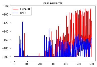
(a) original

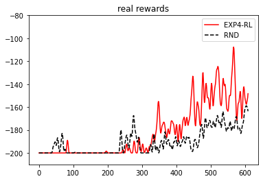
(b) smooth

Figure 1: The performance of Algorithm 3 and RND measured by the epoch-wise reward on Mountain Car

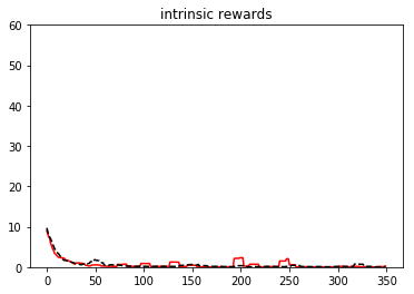
(a) small

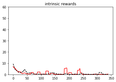
(b) medium

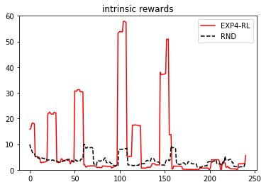
(c) large

Figure 2: The performance of Algorithm 3 and RND measured by intrinsic reward without parallel environments with three different burn-in periods

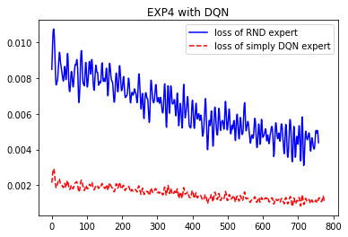
(a) $Q$-network losses with 0.25 update

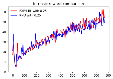
(b) Intrinsic reward after smoothing with 0.25 update

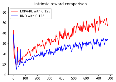
(c) Intrinsic reward after smoothing with 0.125

Figure 3: The performance of Algorithm 3 and RND with 10 parallel environments and with RND update probability 0.25 and 0.125, measured by loss and intrinsic reward.

We next compare EXP4-RL and RND with 10 parallel environments and different RND update probabilities in Figure 3. The experiences are generated by the 10 parallel environments.

Figure 3a shows that both experts in EXP4-RL are learning with decreasing losses of their $Q$-networks. The drop is steeper for the RND expert but it starts with a higher loss. With RND update probability 0.25 in Figure 3b we observe that EXP4-RL and RND are very close when RND exhibits high exploration. When RND is at its local minima, EXP4-RL outperforms it. Usually these local minima are driven by sticking to local maxima and then training the model intensively at local maxima, typical of the RND local exploration behavior. EXP4-RL improves on RND as training progresses, e.g. the improvement after 550 epochs is higher than the one between epochs 250 and 550. In terms for AUC, this is expressed by 1.6% and 3.5%, respectively. Overall, EXP4-RL improves RND local minima of exploration, keeps high exploration of RND and induces a smoother global exploration.

With the update probability of 0.125 in Figure 3c, EXP4-RL almost always outperforms RND with a notable difference. The improvement also increases with epochs and is dramatically larger at RND’s local minima. These local minima appear more frequently in training of RND, so our improvement is more significant as well as crucial. The relative AUC improvement is 49.4%. The excellent performance in Figure 3c additionally shows that EXP4-RL improves RND with global exploration by improving local minima of RND or not staying at local maxima.

Overall, with either 0.25 or 0.125, EXP4-RL incentivizes global exploration on RND by not getting stuck in local exploration maxima and outperforms RND exploration aggressively. With 0.125 the improvement with respect to RND is more significant and steady. This experimental evidence verifies our intuition behind EXP4-RL and provides excellent support for it. With experts being more advanced RL exploration algorithms, e.g. DORA, EXP4-RL can bring additional possibilities.

Appendix A Details about numerical experiments

A.1 Mountain Car

For the Mountain Car experiment, we use the Adam optimizer with the $2\cdot 10^{-4}$ learning rate. The batch size for updating models is 64 with the replay buffer size of 10,000. The remaining parameters are as follows: the discount factor for the $Q$-networks is 0.95, the temperature parameter $\tau$ is 0.1, $\eta$ is 0.05, and $\epsilon$ is decaying exponentially with respect to the number of steps with maximum 0.9 and minimum 0.05. The length of one epoch is 200 steps. The target networks load the weights and biases of the trained networks every 400 steps. Since a reward upper bound is known in advance, we use $n_{r}=1$.

We next introduce the structure of neural networks that are used in the experiment. The neural networks of both experts are linear. For the RND expert, it has the input layer with 2 input neurons, followed by a hidden layer with 64 neurons, and then a two-headed output layer. The first output layer represents the $Q$ values with 64 hidden neurons as input and the number of actions output neurons, while the second output layer corresponds to the intrinsic values, with 1 output neuron. For the DQN expert, the only difference lies in the absence of the second output layer.

A.2 Montezuma’s Revenge

For the Montezuma’s Revenge experiment, we use the Adam optimizer with the $10^{-5}$ learning rate. The other parameters read: the mini batch size is 4, replay buffer size is 1,000, the discount factor for the $Q$-networks is 0.999 and the same valus is used for the intrinsic value head, the temperature parameter $\tau$ is 0.1, $\eta$ is 0.05, and $\epsilon$ is increasing exponentially with minimum 0.05 and maximum 0.9. The length of one epoch is 100 steps. Target networks are updated every 300 steps. Pre-normalization is 50 epochs and the weights for intrinsic and extrinsic values in the first network are 1 and 2, respectively. The upper bound on reward is set to be constant $n_{r}=1$.

For the structure of neural networks, we use CNN architectures since we are dealing with videos. More precisely, for the $Q$-network of the DQN expert in EXP4-RL and the predictor network $\hat{f}$ for computing the intrinsic rewards, we use Alexnet Krizhevsky et al. [2012] pretrained on ImageNet Deng et al. [2009]. The number of output neurons of the final layer is 18, the number of actions in Montezuma. For the RND baseline and RND expert in EXP4-RL, we customize the $Q$-network with different linear layers while keeping all the layers except the final layer of pretrained Alexnet. Here we have two final linear layers representing two value heads, the extrinsic value head and the intrinsic value head. The number of output neurons in the first value head is again 18, while the second value head is with 1 output neuron.

More details about the setup of the experiment on Montezuma’s Revenge are elaborated as follows. The experiment of RND with PPO in Burda et al. [2018] uses many more resources, such as 1024 parallel environments and runs 30,000 epochs for each environment. Parallel environments generate experiences simultaneously and store them in the replay buffer. Our computing environment allows at most 10 parallel environments. For the DQN-version of RND, we use the same settings as Burda et al. [2018], such as observation normalization, intrinsic reward normalization and random initialization. RND update probability is the proportion of experience in the replay buffer that are used for training the intrinsic model $\hat{f}$ in RND Burda et al. [2018]. Here in our experiment, we compare the performance under 0.125 and 0.25 RND update probability.

Appendix B Proof of results in Section 3.1

We first present two lemmas that characterize the relationships among our EXP4.P estimations, the true rewards, and the reward gained by EXP4.P, building on which we establish an optimal sublinear regret of EXP4.P with high probability in the bounded case.

The estimated reward of expert $i$ and the gained reward by the EXP4.P algorithm is denoted by $\hat{G}_{i}=\sum_{t=1}^{T}\hat{z}_{i}(t)$ and $G_{EXP4.P}=\sum_{t=1}^{T}y(t)=\sum_{t=1}^{T}r_{i_{t}}^{t}$, respectively.

For simplicity, we denote

$$\hat{\sigma}_{i}(t+1)=\sqrt{NT}+\sum_{l=1}^{t}\left(\dfrac{1}{\left(\frac{w_{i}(l)}{\sum_{j}w_{j}(l)}+\frac{\gamma}{K}\right)\cdot\sqrt{NT}}\right)$$

$$U=\max_{i}(\hat{G}_{i}+\alpha\cdot\hat{\sigma}_{i}(T+1)),\quad q_{i}(t)=\frac{w_{i}(t)}{\sum_{j}w_{j}(t)}.$$

Let $\alpha$ be the parameter specified in Algorithm $3$. The lemmas read as follows.

Lemma 1.

If   $2\sqrt{K\ln{\frac{NT}{\delta}}}\leq\alpha\leq 2\sqrt{NT}$ and $\gamma<\frac{1}{2}$,  then $P(\exists\;i,\hat{G}_{i}+\alpha\cdot\hat{\sigma}_{i}(T+1)<G_{i})\leq\delta.$

Lemma 2.

If   $\alpha\leq 2\sqrt{NT}$,   then $G_{EXP4.P}\geq\left(1-(1+\frac{2N}{3})\gamma\right)\cdot U-\frac{3K}{\gamma}\ln{N}-2\alpha K\sqrt{NT}-2\alpha^{2}.$

B.1 Proof of Lemma 1

Proof.

Let us denote $s_{t}=\frac{\alpha}{2\hat{\sigma}_{i}(t+1)}$. Since $\alpha\leq 2\sqrt{NT}$ by assumption and $\hat{\sigma}_{i}(t+1)\geq\sqrt{NT}$ by its definition, we have that $s_{t}\leq 1$. Meanwhile,

$$\quad P\left(\hat{G}_{i}+\alpha\hat{\sigma}_{i}(T+1)<G_{i}\right)$$

$$=P\left(\sum_{t=1}^{T}\left(z_{i}(t)-\hat{z}_{i}(t)\right)-\frac{\alpha\hat{\sigma}_{i}(T+1)}{2}>\frac{\alpha\hat{\sigma}_{i}(T+1)}{2}\right)$$

$$\leq P\left(\frac{1}{K}s_{T}\sum_{t=1}^{T}\left(z_{i}(t)-\hat{z}_{i}(t)-\frac{\alpha}{2\left(q_{i}(t)+\frac{\gamma}{K}\right)\sqrt{NT}}\right)>\frac{\alpha^{2}}{4K}\right)$$

$$\leq e^{-\frac{\alpha^{2}}{4K}}E\left[\exp{\left(\frac{s_{T}}{K}\sum_{t=1}^{T}\left(z_{i}(t)-\hat{z}_{i}(t)-\frac{\alpha}{2\left(q_{i}(t)+\frac{\gamma}{K}\right)\sqrt{NT}}\right)\right)}\right]$$ (1)

where the first inequality holds by multiplying $\frac{1}{K}s_{T}=\frac{1}{K}\cdot\frac{\alpha}{2\hat{\sigma}_{i}(T+1)}$ on both sides and then using the fact that $\hat{\sigma}_{i}(T+1)>\sum_{t=1}^{T}\left(\dfrac{1}{\left(q_{i}(t)+\frac{\gamma}{K}\right)\cdot\sqrt{NT}}\right)$ and the second one holds by the Markov’s inequality.

We introduce variable $V_{t}=\exp{\left(\frac{s_{t}}{K}\sum_{t^{\prime}=1}^{t}\left(z_{i}(t^{\prime})-\hat{z}_{i}(t^{\prime})-\frac{\alpha}{2\left(q_{i}(t^{\prime})+\frac{\gamma}{K}\right)\sqrt{NT}}\right)\right)}$ for any $t=1,\ldots,T$. Probability (B.1) can be expressed as $e^{-\frac{\alpha^{2}}{4K}}E\left[V_{T}\right]$. We denote $\mathcal{F}_{t-1}$ as the filtration of the past $t-1$ observations. Note that $V_{t}=\exp{\left(\frac{s_{t}}{K}\left(z_{i}(t)-\hat{z}_{i}(t)-\frac{\alpha}{2\left(q_{i}(t)+\frac{\gamma}{K}\right)\sqrt{NT}}\right)\right)}\cdot V_{t-1}^{\frac{s_{t}}{s_{t-1}}}$ and $s_{t}$ is deterministic given $\mathcal{F}_{t-1}$ since it depends on $q_{i}(\tau)$ up to time $t$ and $q_{i}(t)$ is computed by the past $t-1$ rewards.

Therefore, we have

$$E[V_{t}|\mathcal{F}_{t-1}]$$

$$=E\left[\exp{\left(\frac{s_{t}}{K}\left(z_{i}(t)-\hat{z}_{i}(t)-\frac{\alpha}{2\left(q_{i}(t)+\frac{\gamma}{K}\right)\sqrt{NT}}\right)\right)}\cdot\left(V_{t-1}\right)^{\frac{s_{t}}{s_{t-1}}}|\mathcal{F}_{t-1}\right]$$

$$=E_{t}\left[\exp{\left(\frac{s_{t}}{K}\left(z_{i}(t)-\hat{z}_{i}(t)-\frac{\alpha}{2\left(q_{i}(t)+\frac{\gamma}{K}\right)\sqrt{NT}}\right)\right)}\right]\cdot\left(V_{t-1}\right)^{\frac{s_{t}}{s_{t-1}}}$$

$$\leq E_{t}\left[\exp{\left(\frac{s_{t}}{K}\left(z_{i}(t)-\hat{z}_{i}(t)-\frac{s_{t}}{q_{i}(t)+\frac{\gamma}{K}}\right)\right)}\cdot\left(V_{t-1}\right)^{\frac{s_{t}}{s_{t-1}}}\right]$$

$$\leq E_{t}\left[1+\frac{s_{t}\left(z_{i}(t)-\hat{z}_{i}(t)\right)}{K}+\frac{s_{t}^{2}\left(z_{i}(t)-\hat{z}_{i}(t)\right)^{2}}{K^{2}}\right]\exp{\left(-\frac{s_{t}^{2}}{K\left(q_{i}(t)+\frac{\gamma}{K}\right)}\right)}\cdot\left(V_{t-1}\right)^{\frac{s_{t}}{s_{t-1}}}$$ (2)

where the first inequality holds by using the fact that

$$\alpha=2s_{t}\cdot\hat{\sigma}_{i}(t+1)\geq 2s_{t}\cdot\sqrt{NT}\geq s_{t}\cdot\sqrt{NT}$$

by its definition and the second inequality holds since $e^{x}\leq 1+x+x^{2}$ for $x<1$ which is guaranteed by $s_{t}<1$ and $z_{i}(t)-\hat{z}_{i}(t)<1$. The latter one holds by $1\geq r>0$ and $x_{i}(t)-\hat{x}_{i}(t)=(1-\frac{1}{p})x_{i_{t}}(t)\leq 1$ for $x_{i_{t}}(t)>0$ and

$$z_{i}(t)-\hat{z}_{i}(t) =\sum_{j=1}^{K}\xi_{i}^{j}(t)(x_{i}(t)-\hat{x}_{i}(t))$$

$$=\sum_{j\neq i_{t}}\xi_{i}^{j}(t)x_{j}(t)+\xi_{i}^{i_{t}}(t)(x_{i}(t)-\hat{x}_{i}(t))$$

$$\leq\sum_{j\neq i_{t}}\xi_{i}^{j}(t)+\xi_{i}^{i_{t}}(t)$$

$$=\sum_{j=1}^{K}\xi_{i}^{j}(t)=1$$

Meanwhile,

$$E[\hat{z}_{i}(t)]\\ =E\left[\sum_{j=1}^{K}\xi_{i}^{j}(t)\hat{x}_{j}(t)\right]\\ =\sum_{j=1}^{K}\xi_{i}^{j}(t)E[\hat{x}_{j}(t)]\\ =\sum_{j=1}^{K}\xi_{i}^{j}(t)\cdot x_{j}(t)\\ =z_{i}(t)$$

and

$$\quad E\left[(\hat{z}_{i}(t)-z_{i}(t))^{2}\right]$$

$$=E\left[\left(\sum_{j=1}^{K}\xi_{i}^{j}(t)\left(\hat{x}_{j}(t)-x_{j}(t)\right)\right)^{2}\right]$$

$$\leq K\sum_{j=1}^{K}\left(\xi_{i}^{j}(t)\right)^{2}E\left[(\hat{x}_{j}(t)-x_{j}(t))^{2})\right]$$

$$=K\sum_{j=1}^{K}\left(\xi_{i}^{j}(t)\right)^{2}\cdot\left(\frac{p_{j}(t)\left(x_{j}(t)\right)^{2}(1-p_{j}(t))}{p_{j}(t)}+(1-p_{j}(t))\left(x_{j}(t)\right)^{2}\right)$$

$$=K\sum_{j=1}^{K}\left(\xi_{i}^{j}(t)\right)^{2}\cdot 2(1-p_{j}(t))\left(x_{j}(t)\right)^{2}$$

$$\leq K\sum_{j=1}^{K}\left(\xi_{i}^{j}(t)\right)^{2}\cdot\frac{1-\gamma}{p_{j}(t)}$$

where the first inequality holds by the Cauchy Schwarz inequality and the second inequality holds by the fact that $x_{j}(t)\leq 1$ and $2(1-p)p<1-\gamma$ since $\gamma<\frac{1}{2}$ by assumption.

Note that for any $i,j=1,\ldots,N$ we have

$$p_{j}(t) =(1-\gamma)\sum_{\bar{i}=1}^{N}q_{\bar{i}}(t)\cdot\xi_{\bar{i}}^{j}(t)+\frac{\gamma}{K}$$

$$\geq(1-\gamma)q_{i}(t)\cdot\xi_{i}^{j}(t)+(1-\gamma)\frac{\gamma}{K}\cdot\xi_{i}^{j}(t)$$

$$=(1-\gamma)(q_{i}(t)+\frac{\gamma}{K})\cdot\xi_{i}^{j}(t).$$

since $1-\gamma\leq 1,\xi_{i}^{j}(t)\leq 1$.

We further bound

$$\quad E\left[\left(\hat{z}_{i}(t)-z_{i}(t)\right)^{2}\right]$$

$$\leq K\sum_{j=1}^{K}\left(\xi_{i}^{j}(t)\right)^{2}\cdot\frac{1-\gamma}{p_{j}(t)}$$

$$\leq K\sum_{j=1}^{K}\frac{(1-\gamma)\left(\xi_{i}^{j}(t)\right)^{2}}{(1-\gamma)(q_{i}(t)+\frac{\gamma}{K})\xi_{i}^{j}(t)}$$

$$=K\sum_{j=1}^{K}\frac{\xi_{i}^{j}(t)}{q_{i}(t)+\frac{\gamma}{K}}$$

$$=K\frac{1}{q_{i}(t)+\frac{\gamma}{K}}$$

Then by using (B.1), we have that

$$E[V_{t}|\mathcal{F}_{t-1}] \leq\left(1+\frac{s_{t}^{2}}{K\left(q_{i}(t)+\frac{\gamma}{K}\right)}\right)\exp{\left(-\frac{s_{t}^{2}}{K\left(q_{i}(t)+\frac{\gamma}{K}\right)}\right)}\cdot\left(V_{t-1}\right)^{\frac{s_{t}}{s_{t-1}}}$$

$$\leq\exp{\left(\frac{s_{t}^{2}}{K\left(q_{i}(t)+\frac{\gamma}{K}\right)}-\frac{s_{t}^{2}}{K\left(q_{i}(t)+\frac{\gamma}{K}\right)}\right)}\left(V_{t-1}\right)^{\frac{s_{t}}{s_{t-1}}}$$

$$\leq 1+V_{t-1}$$

where we have first used $1+x\leq e^{x}$ and then $a^{x}\leq 1+a$ for any $x\in[0,1]$ with $x=\frac{s_{t}}{s_{t-1}}\leq 1$. By law of iterated expectation, we obtain

$$E[V_{t}] =E[E[V_{t}|\mathcal{F}_{t-1}]]\leq E[1+V_{t-1}]=1+E[V_{t-1}].$$

Meanwhile, note that

$$E[V_{1}] =\exp{\left(\frac{s_{1}}{K}\left(z_{i}(1)-\hat{z}_{i}(1)-\frac{\alpha}{2\left(q_{i}(1)+\frac{\gamma}{K}\right)\sqrt{NT}}\right)\right)}$$

$$=\exp{\left(\frac{s_{1}}{K}\left(z_{i}(1)-\hat{z}_{i}(1)-\frac{\alpha}{2\left(\frac{1}{N}+\frac{\gamma}{K}\right)\sqrt{NT}}\right)\right)}$$

$$\leq\exp{\left(\frac{s_{1}}{K}\left(-\frac{\alpha}{2\left(\frac{1}{N}+\frac{\gamma}{K}\right)\sqrt{NT}}\right)\right)}<1$$

where the first inequality holds by using the fact that

$$z_{i}(1)-\hat{z}_{i}(1) =\sum_{j=1}^{K}\xi_{i}^{j}(1)x_{j}(1)(1-\frac{1}{(1-\gamma)\frac{1}{N}\sum_{i^{\prime}=1}^{N}\xi_{i^{\prime}}^{j}(1)+\frac{\gamma}{K}})$$

$$\leq\sum_{j=1}^{K}\xi_{i}^{j}(1)(1-\frac{1}{(1-\gamma)+\frac{\gamma}{K}})$$

$$=\frac{(-1+\frac{1}{K})\gamma}{1-\gamma+\frac{\gamma}{K}}<0$$

since $0<x_{j}(1)\leq 1$ and $0\leq\xi_{i^{\prime}}^{j}(1)\leq 1$ and the second inequality is a result of $\alpha>0$, $s_{1}>0$.

Therefore, by induction we have that $E[V_{T}]\leq T$.

To conclude, combining all above, we have that $P\left(\hat{G}_{i}+\alpha\hat{\sigma}_{i}<G_{i}\right)\leq e^{-\frac{\alpha^{2}}{4K}}E[V_{T}]\leq e^{-\frac{\alpha^{2}}{4K}}T$ and the lemma follows as we choose specific $\alpha$ that satisfies $e^{-\frac{\alpha^{2}}{4K}}T\leq\frac{\delta}{N}$, i.e $2\sqrt{K\ln{\frac{NT}{\delta}}}\leq\alpha$. ∎

B.2 Proof of Lemma 2

Proof.

For simplicity, let $\vartheta=\frac{\gamma}{3K}$ and consider any sequence $i_{1},\ldots,i_{T}$ of actions by EXP4.P.

Since $p_{j}(t)>\frac{\gamma}{K}$, we observe

$$\hat{z}_{i}(t)=\sum_{j=1}^{K}\xi_{j}^{i}(t)\hat{x}_{j}(t)\leq\sum_{j=1}^{K}\xi_{j}^{i}(t)\frac{1}{p_{j}(t)}\leq\sum_{j=1}^{K}\xi_{j}^{i}(t)\frac{K}{\gamma}=\frac{K}{\gamma}.$$

Then the term $\vartheta\cdot\left(\hat{z}_{i}(t)+\frac{\alpha}{\frac{w_{i}(t)}{\sum_{j=1}^{N}w_{j}(t)}\sqrt{NT}}\right)$ is less than 1, noting that

$$\quad\vartheta\cdot\left(\hat{z}_{i}(t)+\frac{\alpha}{\left(\frac{w_{i}(t)}{\sum_{j=1}^{N}w_{j}(t)}+\frac{\gamma}{K}\right)\sqrt{NT}}\right)$$

$$=\frac{\gamma}{3K}\left(\hat{z}_{i}(t)+\frac{\alpha}{\left(q_{i}(t)+\frac{\gamma}{K}\right)\sqrt{NT}}\right)$$

$$\leq\frac{\gamma}{3K}\cdot\frac{K}{\gamma}+\frac{\gamma}{3K}\cdot\frac{K}{\gamma}\cdot\frac{\alpha}{\sqrt{NT}}$$

$$\leq\frac{1}{3}+\frac{1}{3}\cdot\frac{2\sqrt{NT}}{\sqrt{NT}}=1.$$

We denote $W_{t}=\sum_{i=1}^{N}w_{i}(t)$, which satisfies

$$\frac{W_{t+1}}{W_{t}} =\sum_{i=1}^{N}\frac{w_{i}(t+1)}{W_{t}}$$

$$=\sum_{i=1}^{N}q_{i}(t)\cdot\exp{\left(\vartheta\cdot\left(\hat{z}_{i}(t)+\frac{\alpha}{\left(\frac{w_{i}(t)}{\sum_{j=1}^{N}w_{j}(t)}+\frac{\gamma}{K}\right)\sqrt{NT}}\right)\right)}$$

$$\leq\sum_{i=1}^{N}q_{i}(t)\cdot\biggl{(}1+\vartheta\hat{z}_{i}(t)+\frac{\alpha\vartheta}{\left(q_{i}(t)+\frac{\gamma}{K}\right)\sqrt{NT}}\quad+$$

$$\qquad\qquad\qquad\qquad 2\vartheta^{2}\left(\hat{z}_{i}(t)\right)^{2}+2\frac{\alpha^{2}\vartheta^{2}}{\left(q_{i}(t)+\frac{\gamma}{K}\right)^{2}NT}\biggl{)}$$

$$=1+\vartheta\sum_{i=1}^{N}q_{i}(t)\hat{z}_{i}(t)+2\vartheta^{2}\sum_{i=1}^{N}q_{i}(t)\left(\hat{z}_{i}(t)\right)^{2}+$$

$$\qquad\qquad\quad\alpha\vartheta\sum_{i=1}^{N}\frac{q_{i}(t)}{\left(q_{i}(t)+\frac{\gamma}{K}\right)\sqrt{NT}}+2\alpha^{2}\vartheta^{2}\sum_{i=1}^{N}\frac{q_{i}(t)}{\left(q_{i}(t)+\frac{\gamma}{K}\right)^{2}NT}$$ (3)

where the last inequality using the facts that $e^{x}<1+x+x^{2}$ for $x<1$ and $2(a^{2}+b^{2})>(a+b)^{2}$. Note that the second term in the above expression satisfies

$$\sum_{i=1}^{N}q_{i}(t)\hat{z}_{i}(t) =\sum_{i=1}^{N}q_{i}(t)\left(\sum_{j=1}^{K}\xi_{i}^{j}(t)\hat{x}_{j}(t)\right)$$

$$=\sum_{j=1}^{K}\left(\sum_{i=1}^{N}q_{i}(t)\xi_{i}^{j}(t)\right)\hat{x}_{j}(t)$$

$$=\sum_{j=1}^{K}\left(\frac{p_{j}(t)-\frac{\gamma}{K}}{1-\gamma}\right)\hat{x}_{j}(t)\leq\frac{x_{i_{t}}(t)}{1-\gamma}$$

Also the third term yields

$$\sum_{i=1}^{N}q_{i}(t)\left(\hat{z}_{i}(t)\right)^{2} =\sum_{i=1}^{N}q_{i}(t)\left(\sum_{j=1}^{K}\xi_{i}^{j}(t)\hat{x}_{j}(t)\right)^{2}$$

$$=\sum_{i=1}^{N}q_{i}(t)\left(\xi_{i}^{i_{t}}\hat{x}_{i_{t}}(t)\right)^{2}$$

$$\leq\hat{x}_{i_{t}}(t)^{2}\frac{p_{i_{t}}(t)}{1-\gamma}\leq\frac{\hat{x}_{i_{t}}(t)}{1-\gamma}.$$

We also note that

$$\alpha\vartheta\sum_{i=1}^{N}\frac{q_{i}(t)}{\left(q_{i}(t)+\frac{\gamma}{K}\right)\sqrt{NT}}\leq\alpha\vartheta\sqrt{\frac{N}{T}}$$

and

$$2\alpha^{2}\vartheta^{2}\sum_{i=1}^{N}\frac{q_{i}(t)}{\left(q_{i}(t)+\frac{\gamma}{K}\right)^{2}NT}\leq 2\alpha^{2}\vartheta^{2}\frac{1}{3\vartheta T}=\frac{2\alpha^{2}\vartheta}{3T}.$$

Plugging these estimates in (B.2), we get

$$\frac{W_{t+1}}{W_{t}}\leq 1+\frac{\vartheta}{1-\gamma}x_{i_{t}}(t)+\frac{2\vartheta^{2}}{1-\gamma}\sum_{j=1}^{K}\hat{x}_{j}(t)+\alpha\vartheta\sqrt{\frac{N}{T}}+\frac{2\alpha^{2}\vartheta}{3T}.$$

Then we note that for any $j$, $\sum_{i=1}^{N}\xi_{i}^{j}(t)\geq\frac{1}{K}$ by the assumption that a uniform expert is included, which gives us that

$$\frac{W_{t+1}}{W_{t}}\leq 1+\frac{\vartheta}{1-\gamma}x_{i_{t}}(t)+\frac{2\vartheta^{2}}{1-\gamma}K\sum_{i=1}^{N}\hat{z}_{i}(t)+\alpha\vartheta\sqrt{\frac{N}{T}}+\frac{2\alpha^{2}\vartheta}{3T}.$$

Since $\ln{\left(1+x\right)}<x$, we have that

$$\ln{\frac{W_{t+1}}{W_{t}}}\leq\frac{\vartheta}{1-\gamma}x_{i_{t}}(t)+\frac{2\vartheta^{2}}{1-\gamma}K\sum_{i=1}^{N}\hat{z}_{i}(t)+\alpha\vartheta\sqrt{\frac{N}{T}}+\frac{2\alpha^{2}\vartheta}{3T}.$$

Then summing over $t$ leads to

$$\ln{\frac{W_{T+1}}{W_{1}}}\leq\frac{\vartheta}{1-\gamma}G_{EXP4.P}+\frac{2\vartheta^{2}}{1-\gamma}K\sum_{i=1}^{N}\hat{G}_{i}(t)+\alpha\vartheta\sqrt{NT}+\frac{2\alpha^{2}\vartheta}{3}.$$

Meanwhile, by initialization we have that

$$\ln{\left(W_{1}\right)} =\ln{\left(Nw_{i}(1)\right)}$$

$$=\ln{\left(N\cdot\exp{\left(\alpha\vartheta\sqrt{NT}\right)}\right)}$$

$$=\ln{N}+\alpha\vartheta\sqrt{NT}.$$

For any $\bar{i}$, we also have

$$\ln{W_{T+1}} =\ln{\sum_{i=1}^{N}w_{i}(T+1)}$$

$$\geq\ln{w_{\bar{i}}(T+1)}$$

$$=\ln{\left(w_{\bar{i}}(T)\exp{\left(\vartheta\left(\hat{z}_{\bar{i}}(T)+\frac{\alpha}{(q_{\bar{i}}(T)+\frac{\gamma}{K})\sqrt{NT}}\right)\right)}\right)}$$

$$=\ln\left(w_{\bar{i}}(1)\prod_{t=1}^{T}\exp{\left(\vartheta\left(\hat{z}_{\bar{i}}(t)+\frac{\alpha}{(q_{\bar{i}}(t)+\frac{\gamma}{K})\sqrt{NT}}\right)\right)}\right)$$

$$=\ln{\left(w_{\bar{i}}(1)\exp{\left(\vartheta\left(\sum_{t=1}^{T}\hat{z}_{\bar{i}}(t)+\sum_{t=1}^{T}\frac{\alpha}{(q_{\bar{i}}(t)+\frac{\gamma}{K})\sqrt{NT}}\right)\right)}\right)}$$

$$=\ln{\left(\exp{(\vartheta\alpha\sqrt{NT})}\exp{\left(\vartheta\left(\sum_{t=1}^{T}\hat{z}_{\bar{i}}(t)+\sum_{t=1}^{T}\frac{\alpha}{(q_{\bar{i}}(t)+\frac{\gamma}{K})\sqrt{NT}}\right)\right)}\right)}$$

$$=\ln{\left(\exp{\left(\vartheta\left(\sum_{t=1}^{T}\hat{z}_{\bar{i}}(t)+\alpha\left(\sqrt{NT}+\sum_{t=1}^{T}\frac{1}{(q_{\bar{i}}(t)+\frac{\gamma}{K})\sqrt{NT}}\right)\right)\right)}\right)}$$

$$=\vartheta\hat{G}_{\bar{i}}+\alpha\vartheta\hat{\sigma}_{\bar{i}}(T+1).$$

Therefore, we have that

$$\vartheta\hat{G}_{\bar{i}}+\alpha\vartheta\hat{\sigma}_{\bar{i}}(T+1)-\ln{N}-\alpha\vartheta\sqrt{NT}\leq\frac{\vartheta}{1-\gamma}G_{EXP4.P}+\frac{2\vartheta^{2}}{1-\gamma}K\sum_{i=1}^{N}\hat{G}_{i}+\alpha\vartheta\sqrt{NT}+\frac{2\alpha^{2}\vartheta}{3}.$$

By re-organizing the terms and then multiplying by $\frac{\bm{1}-\gamma}{\vartheta}$ on both sides, the above expression can be written as

$$G_{EXP4.P} =(1-\gamma)(\hat{G}_{\bar{i}}+\alpha\hat{\sigma}_{\bar{i}}(T+1))$$

$$\qquad\qquad-(1-\gamma)\frac{\ln{N}}{\vartheta}-(1-\gamma)2\alpha\sqrt{NT}-2\vartheta K\sum_{i=1}^{N}\hat{G}_{i}-(1-\gamma)\frac{2\alpha^{2}}{3}$$

$$\geq(1-\gamma)(\hat{G}_{\bar{i}}+\alpha\hat{\sigma}_{\bar{i}}(T+1))-\frac{\ln{N}}{\vartheta}-2\alpha\sqrt{NT}-2\vartheta K\sum_{i=1}^{N}\hat{G}_{i}-2\alpha^{2}$$

Note that the above holds for any $\bar{i}$ and that $\sum_{i=1}^{N}\hat{G}_{i}\leq NU$.

The lemma follows by replacing $\hat{G}_{\bar{i}}+\alpha\hat{\sigma}_{\bar{i}}(T+1)$ with $U$ by selecting $\bar{i}$ to be the expert where $U$ achieves maximum and $\sum_{i=1}^{N}\hat{G}_{i}$ with $NU$.

∎

B.3 Proof of Theorem 1

Proof.

Without loss of generality, we assume $\delta\geq NTe^{-\frac{NT}{K}}$ and $T\geq\max{\left(\frac{3(2N+3)K\ln{N}}{3},\frac{36K\ln{N}}{2N+3}\right)}$. If either of the conditions does not hold, it is easy to observe that the theorem holds as follows. Since reward is between 0 and 1, the regret is always less or equal to $T$. On the other hand, if one of these conditions is not met, a straightforward derivation shows that the last term in the upper bound of the regret statement in the theorem is greater or equal to $T$.

By Lemma 2, we have that

$$G_{EXP4.P}\geq\left(1-(1+\frac{2N}{3})\gamma\right)\cdot U-\frac{3K}{\gamma}\ln{N}-2\alpha K\sqrt{NT}-2\alpha^{2}.$$

Since $\delta\geq NTe^{-\frac{NT}{K}}$, we have $2\sqrt{K\ln{\left(\frac{NT}{\delta}\right)}}\leq 2\sqrt{NT}$. Then Lemma 1 gives us that

$$U\geq G_{max}=\max_{i}{G_{i}},\text{ with probability at least }1-\delta$$

when $\gamma<\frac{1}{2}$.

Combining the two together and using the fact that $G_{max}\leq T$, we get

$$G_{max}-G_{EXP4.P} \leq\left(\left(\frac{2N}{3}+1\right)\gamma\right)G_{max}+\frac{3K\ln{N}}{\gamma}+2\alpha K\sqrt{NT}+2\alpha^{2}$$

$$\leq\left(\left(\frac{2N}{3}+1\right)\gamma\right)T+\frac{3K\ln{N}}{\gamma}+2\alpha K\sqrt{NT}+2\alpha^{2},$$ (4)

which holds with probability at least $1-\delta$ when $1-\frac{2N+3}{3}\cdot\gamma\geq 0$

Let $\gamma=\sqrt{\frac{3K\ln{N}}{T\left(\frac{2N}{3}+1\right)}}$ and $\alpha=2\sqrt{K\ln{\left(\frac{NT}{\delta}\right)}}$. Note that $T\geq\max{\left(\frac{3(2N+3)K\ln{N}}{3},\frac{36K\ln{N}}{2N+3}\right)}$, which implies that

$$1-\frac{2N+3}{3}\cdot\gamma=1-\frac{2N+3}{3}\cdot\sqrt{\frac{3K\ln{N}}{T\left(\frac{2N}{3}+1\right)}}\geq 0,$$

$$\gamma=\sqrt{\frac{3K\ln{N}}{T\left(\frac{2N}{3}+1\right)}}<\frac{1}{2}.$$

By plugging them into the right hand side of (B.3), we get

$$\quad G_{max}-G_{EXP4.P}$$

$$\leq 2\sqrt{3KT\left(\frac{2N}{3}+1\right)\ln{N}}+4K\sqrt{KNT\ln{\left(\frac{NT}{\delta}\right)}}+8K\ln{\left(\frac{NT}{\delta}\right)}$$

$$\leq 2\sqrt{3KT\left(\frac{2N}{3}+1\right)\ln{N}}+4K\sqrt{KNT\ln{\left(\frac{NT}{\delta}\right)}}+8NK\ln{\left(\frac{NT}{\delta}\right)}$$

with probability $1-\delta$, i.e. $R_{T}=G_{max}-G_{EXP4.P}\leq O^{*}(\sqrt{T})$, with probability at least $1-\delta$.

∎

B.4 Proof of Theorem 2

Proof.

Since the rewards can be unbounded in this setting, we consider truncating the reward with any $\Delta>0$ for any arm $i$ by $r^{t}_{i}=\bar{r}^{t}_{i}+\hat{r}^{t}_{i}$ where

$\bar{r}^{t}_{i}=r^{t}_{i}\cdot\mathds{1}_{(-\Delta\leq r^{t}_{i}\leq\Delta)},\hat{r}^{t}_{i}=r^{t}_{i}\cdot\mathds{1}_{(|r^{t}_{i}|>\Delta)}$.

Then for any parameter $0<\eta<1$, we choose such $\Delta$ that satisfies

$$P(r^{t}_{i}=\bar{r}^{t}_{i},i\leq K)=P(-\Delta\leq r^{t}_{1}\leq\Delta,\ldots,-\Delta\leq r^{t}_{K}\leq\Delta)$$

$$=\int_{-\Delta}^{\Delta}\int_{-\Delta}^{\Delta}\ldots\int_{-\Delta}^{\Delta}f(x_{1},\ldots,x_{K})dx_{1}\ldots dx_{K}\geq 1-\eta\>.$$ (5)

The existence of such $\Delta=\Delta(\eta)$ follows from elementary calculus.

Let $A=\{|r_{i}^{t}|\leq\Delta$ for every $i\leq K,t\leq T\}$. Then the probability of this event is

$P(A)=P(r^{t}_{i}=\bar{r}^{t}_{i},i\leq K,t\leq T)\geq(1-\eta)^{T}$.

With probability $(1-\eta)^{T}$, the rewards of the player are bounded in $[-\Delta,\Delta]$ throughout the game. Then $R^{c,B}_{T}=\max_{i}\sum_{t=1}^{T}\sum_{j=1}^{K}\xi_{i}^{j}(t)\bar{r}^{t}_{j}-\sum_{t=1}^{T}\bar{r}^{i}_{t}\leq T\cdot\Delta-\sum_{t=1}^{T}r_{t}$ is the regret under event $A$, i.e. $R_{T}=R^{c,B}_{T}$ with probability $(1-\eta)^{T}$. For the EXP4.P algorithm and $R^{c,B}_{T}$ with rewards $\bar{r}_{j}^{t}=\frac{\bar{r}_{j}^{t}+\Delta}{\Delta}$ satisfying $0<\bar{r}_{j}^{t}<1$, for every $\delta>0$, according to Theorem 2 , we have

$$R^{c,B}_{T}\leq 4\Delta(\eta)\left(2\sqrt{3KT\left(\frac{2N}{3}+1\right)\ln{N}}+4K\sqrt{KNT\ln{\left(\frac{NT}{\delta}\right)}}+8NK\ln{\left(\frac{NT}{\delta}\right)}\right).$$

Then we have

$$R_{T}\leq 4\Delta(\eta)\left(2\sqrt{3KT\left(\frac{2N}{3}+1\right)\ln{N}}+4K\sqrt{KNT\ln{\left(\frac{NT}{\delta}\right)}}+8NK\ln{\left(\frac{NT}{\delta}\right)}\right)$$

$$\text{ with probability }(1-\delta)\cdot(1-\eta)^{T}.$$

∎

B.5 Proof of Theorem 3

Lemma 3.

For any non-decreasing differentiable function $\Delta=\Delta(T)>0$ satisfying

$\lim_{T\to\infty}\frac{\Delta(T)^{2}}{\log(T)}=\infty$,  $\lim_{T\to\infty}\Delta^{\prime}(T)\leq C_{0}<\infty$,

and any $0<\delta<1,a>2$ we have

$$P\left(R_{T}^{c}\leq\Delta(T)\cdot\log(1/\delta)\cdot O^{*}(\sqrt{T})\right)\geq(1-\delta)\left(1-\frac{1}{T^{a}}\right)^{T}$$

for any $T$ large enough.

Proof.

Let $a>2$ and let us denote

$$F(y)=\int_{-y}^{y}f(x_{1},x_{2},\ldots,x_{K})dx_{1}dx_{2}\ldots dx_{K},$$

$$\zeta(T)=F\left(\Delta(T)\cdot\mathbf{1}\right)-\left(1-\frac{1}{T^{a}}\right)$$

for $y\in\mathds{R}^{K}$ and $\mathbf{1}=(1,\ldots,1)\in\mathds{R}^{K}$. Let also $y_{-i}=(y_{1},\ldots,y_{i-1},y_{i+1},\ldots,y_{K})$ and $x|_{x_{i}=y}=(x_{1},\ldots,x_{i-1},y,x_{i+1},\ldots,x_{K})$. We have $\lim_{T\to\infty}\zeta(T)=0$.

The gradient of $F$ can be estimated as

$$\nabla F \leq\left(\int_{-y_{-1}}^{y_{-1}}f\left(x|_{x_{1}=y_{1}}\right)dx_{2}\ldots d{x_{K}},\ldots,\int_{-y_{-K}}^{y_{-K}}f\left(x|_{x_{K}=y_{K}}\right)dx_{1}\ldots d{x_{K-1}}\right).$$

According to the chain rule and since $\Delta^{\prime}(T)\geq 0$, we have

$$\frac{dF(\Delta(T)\cdot\mathbf{1})}{dT} \leq\int_{-\Delta(T)\cdot\mathbf{1}_{-1}}^{\Delta(T)\cdot\mathbf{1}_{-1}}f\left(x|_{x_{1}=\Delta(T)}\right)dx_{2}\ldots d{x_{K}}\cdot\Delta^{\prime}(T)+$$

$$\qquad\ldots+\int_{-\Delta(T)\cdot\mathbf{1}_{-K}}^{\Delta(T)\cdot\mathbf{1}_{-K}}f\left(x|_{x_{K}=\Delta(T)}\right)dx_{1}\ldots d{x_{K-1}}\cdot\Delta^{\prime}(T).$$

Next we consider

$$\int_{-\Delta(T)\mathbf{1}_{-i}}^{\Delta(T)\mathbf{1}_{-i}}f\left(x|_{x_{i}=\Delta(T)}\right)dx_{1}\ldots dx_{i-1}dx_{i+1}\ldots dx_{K}$$

$$\leq e^{-\frac{1}{2}a_{ii}(\Delta(T))^{2}+\mu_{i}\Delta(T)}\cdot\int_{-\Delta(T)\mathbf{1}_{-i}}^{\Delta(T)\mathbf{1}_{-i}}e^{g\left(x_{-i}\right)}dx_{1}\ldots dx_{i-1}dx_{i+1}\ldots dx_{K}.$$

Here $e^{g(x_{-i})}$ is the conditional density function given $x_{i}=\Delta(T)$ and thus $\int_{-\Delta(T)\mathbf{1}_{-i}}^{\Delta(T)\mathbf{1}_{-i}}e^{g\left(x_{-i}\right)}dx_{1}\ldots dx_{i-1}dx_{i+1}\ldots dx_{K}\leq 1$. We have

$$\int_{-\Delta(T)\mathbf{1}_{-i}}^{\Delta(T)\mathbf{1}_{-i}}f\left(x|_{x_{i}=\Delta(T)}\right)dx_{1}\ldots dx_{i-1}dx_{i+1}\ldots dx_{K}$$

$$\leq e^{-\frac{1}{2}a_{ii}(\Delta(T))^{2}+\mu_{i}\Delta(T)}$$

$$\leq e^{-\frac{1}{2}\min_{j}a_{jj}(\Delta(T))^{2}+\max_{j}{\mu_{j}}\Delta(T)}.$$

Then for $T\geq T_{0}$ we have $\Delta^{\prime}_{T}\leq C_{0}+1$ and in turn

$\zeta^{\prime}(T)\leq(C_{0}+1)\cdot K\cdot e^{-\frac{1}{2}\min_{j}{a_{jj}}(\Delta(T))^{2}+\max_{j}{\mu_{j}}\Delta(T)}-a\cdot T^{-a-1}$.

Since we only consider non-degenerate sub-Gaussian bandits with $\min{a_{ii}}>0$, $\mu_{i}$ are constants and $\Delta(T)\rightarrow\infty$ as $T\rightarrow\infty$ according to the assumptions in Lemma 3, there exits $C_{1}>0$ and $T_{1}$ such that

$e^{-\frac{1}{2}\min_{j}{a_{jj}}(\Delta(T))^{2}+\max_{j}{\mu_{j}}\Delta(T)}\leq e^{-C_{1}\Delta(T)^{2}}$ for every $T>T_{1}$.

Since $\lim_{T\to\infty}\frac{\Delta(T)^{2}}{\log(T)}=\infty$, we have

$\Delta(T)^{2}>\frac{2(a+1)}{C_{1}}\cdot\log(T)$ for $T>T_{2}$.

These give us that

$$\zeta(T)^{\prime} \leq(C_{0}+1)Ke^{-2(a+1)\log T}-aT^{-a-1}$$

$$=(C_{0}+1)Ke^{-2(a+1)\log T}-ae^{-(a+1)\log T}$$

$$<0\text{ for }T\geq T_{3}\geq\max(T_{0},T_{1},T_{2}).$$

This concludes that $\zeta^{\prime}(T)<0$ for $T\geq T_{3}$. We also have $\lim_{T\to\infty}\zeta(T)=0$ according to the assumptions. Therefore, we finally arrive at $\zeta(T)>0$ for $T\geq T_{3}$. This is equivalent to

$$\int_{-\Delta(T)\cdot\mathbf{1}}^{\Delta(T)\cdot\mathbf{1}}f\left(x_{1},\ldots,x_{K}\right)dx_{1}\ldots dx_{K}\geq 1-\frac{1}{T^{a}},$$

i.e. the rewards are bounded by $\Delta(T)$ with probability $1-\frac{1}{T^{a}}$. Then by the same argument for $T$ large enough as in the proof of Theorem 2, we have

$$P\left(R_{T}^{c}\leq\Delta(T)\cdot\log(1/\delta)\cdot O^{*}(\sqrt{T})\right)\geq(1-\delta)(1-\frac{1}{T^{a}})^{T}.$$

∎

Proof of Theorem 3.

In Lemma 3, we choose $\Delta(T)=\log(T)$, which meets all of the assumptions. The result now follows from $\log T\cdot O^{*}(\sqrt{T})=O^{*}(\sqrt{T})$, Lemma 3 and Theorem 2. ∎

B.6 Proof of Theorem 4

We first list 3 known lemmas. The following lemma by Duchi [2009] provides a way to bound deviations.

Lemma 4.

For any function class $F$, and i.i.d. random variable $\{x_{1},x_{2},\ldots,x_{T}\}$, the result

$E_{x}\left[\sup_{f\in F}\left|E_{x}f-\frac{1}{T}\sum_{t=1}^{T}f\left(x_{t}\right)\right|\right]\leq 2R_{T}^{c}(F)$

holds where $R_{T}^{c}(F)=E_{x,\sigma}\left[\sup_{f}\left|\frac{1}{T}\sum_{t=1}^{T}\sigma_{t}f\left(x_{t}\right)\right|\right]$ and $\sigma_{t}$ is a $\{-1,1\}$ random walk of $t$ steps.

The following result holds according to Balcan [2011].

Lemma 5.

For any subclass $A\subset F$, we have $\hat{R}^{c}_{T}\leq R(A,T)\cdot\frac{\sqrt{2\log{|A|}}}{T}$, where $R(A,T)=\sup_{f\in A}\left(\sum_{t=1}^{T}f^{2}(x_{t})\right)^{\frac{1}{2}}$ and $\hat{R}^{c}_{T}=\sup_{f}\left|\frac{1}{T}\sum_{t=1}^{T}\sigma_{t}f\left(x_{t}\right)\right|$.

The following lemma is listed in the Appendix A of Chatterjee [2014].

Lemma 6.

For i.i.d. $\sigma^{2}$-sub-Gaussian random variables $\{Y_{1},Y_{2},\ldots,Y_{T}\}$, we have

$E\left[\max_{1\leq t\leq T}|Y_{t}|\right]\leq\sigma\sqrt{2\log T}+\frac{4\sigma}{\sqrt{2\log T}}.$

Proof of Theorem 4.

Let us define $F=\{f_{i,t}:x\rightarrow\sum_{j=1}^{K}\xi_{i}^{j}(t)x_{j}(t)|i=1,2,\ldots,N;t=1,\ldots,T\}$. Let $x_{t}=x(t)=(r^{t}_{1},r^{t}_{2},\ldots,r^{t}_{K})$ where $r^{t}_{j}$ is the reward of arm $j$ at step $t$ and let $a_{t}$ be the arm selected at time $t$ by EXP4.P. Then for any $f_{i,t}\in F$, $f_{i,t}(x_{t_{i}})=I_{t=t_{i}}\sum_{j=1}^{K}\xi_{i}^{j}(t)x_{j}(t)$. In sub-Gaussian bandits, $\{x_{1},x_{2},\ldots,x_{T}\}$ are i.i.d. random variables since the sub-Gaussian distribution $\sigma^{2}-\mathcal{N}(\mu,\Sigma)$ is invariant to time and independent of time. Then by Lemma 4, we have

$E\left[\max_{i,t}\left|\sum_{j=1}^{K}\xi_{i}^{j}(t)\mu_{j}-\frac{1}{T}\sum_{t=1}^{T}\sum_{j=1}^{K}\xi_{i}^{j}(t)r^{t}_{j}\right|\right]\leq 2R_{T}(F)$.

We consider

$$\begin{split}E\left[\left|R^{\prime}_{T}-R_{T}\right|\right]&=E\left[\left|\sum_{t=1}^{T}\max_{i}\sum_{j=1}^{K}\xi_{i}^{j}(t)\mu_{j}-\sum_{t=1}^{T}\mu_{a_{t}}-\left(\max_{i}\sum_{t=1}^{T}\sum_{j=1}^{K}\xi_{i}^{j}(t)r^{t}_{j}-\sum_{t=1}^{T}r^{t}_{a_{t}}\right)\right|\right]\\ &\leq E\left[\left|\sum_{t=1}^{T}\max_{i}\sum_{j=1}^{K}\xi_{i}^{j}(t)\mu_{j}-\max_{i}\sum_{t^{\prime}=1}^{T}\sum_{j=1}^{K}\xi_{i}^{j}(t^{\prime})r^{t^{\prime}}_{j}\right|\right]\\ &\qquad\qquad\qquad\qquad+E\left[\left|\left(\sum_{t=1}^{T}\mu_{a_{t}}-\sum_{t=1}^{T}r^{t}_{a_{t}}\right)\right|\right]\\ &=E\left[\left|\sum_{t=1}^{T}\max_{i}\left(\sum_{j=1}^{K}\xi_{i}^{j}(t)\mu_{j}-\max_{i}\frac{1}{T}\sum_{t^{\prime}=1}^{T}\sum_{j=1}^{K}\xi_{i}^{j}(t^{\prime})r^{t^{\prime}}_{j}\right)\right|\right]\\ &\qquad\qquad\qquad\qquad+E\left[\left|\left(\sum_{t=1}^{T}\mu_{a_{t}}-\sum_{t=1}^{T}r^{t}_{a_{t}}\right)\right|\right]\\ &\leq E\left[\sum_{t=1}^{T}\max_{i}\left|\sum_{j=1}^{K}\xi_{i}^{j}(t)\mu_{j}-\frac{1}{T}\sum_{t^{\prime}=1}^{T}\sum_{j=1}^{K}\xi_{i}^{j}(t^{\prime})r^{t^{\prime}}_{j}\right|\right]+\mathrm{E}\left[\left|\sum_{t=1}^{T}\mu_{a_{t}}-\sum_{t=1}^{T}r^{t}_{a_{t}}\right|\right]\\ &\leq E\left[T\cdot\max_{i,t}\left|\sum_{j=1}^{K}\xi_{i}^{j}(t)\mu_{j}-\frac{1}{T}\sum_{t^{\prime}=1}^{T}\sum_{j=1}^{K}\xi_{i}^{j}(t^{\prime})r^{t^{\prime}}_{j}\right|\right]+\mathrm{E}\left[\left|\sum_{t=1}^{T}\mu_{a_{t}}-\sum_{t=1}^{T}r^{t}_{a_{t}}\right|\right]\\ &\leq 2TR_{T}(F)+2T_{1}R_{T_{1}}(F)+\cdots+2T_{K}R_{T_{K}}(F)\end{split}$$ (6)

where $T_{i}$ is the number of pulls of arm $i$. Clearly $T_{1}+T_{2}+\ldots+T_{K}=T$. By Lemma 5 with $A=F$ which has cardinality of $NT$ we get

$$R_{T}^{c}(F)=E\left[\hat{R}_{T}^{c}(F)\right]\leq E[R(F,T)]\cdot\frac{\sqrt{2\log\left(NT\right)}}{T},$$

$$R_{T_{j}}^{c}(F)\leq E\left[R\left(F,T_{j}\right)\right]\cdot\frac{\sqrt{2\log\left(NT\right)}}{T_{j}}\qquad j=\{1,2,,\ldots,K\}.$$

Since $R(F,T)$ is increasing in $T$ and $T_{j}\leq T$, we have $R_{T_{j}}^{c}(F)\leq E\left[R\left(F,T\right)\right]\cdot\frac{\sqrt{2\log\left(NT\right)}}{T_{j}}$.

We next bound the expected deviation $E\left[\left|R^{\prime}_{T}-R_{T}\right|\right]$ based on (6) as follows

$$E\left[\left|R^{\prime}_{T}-R_{T}\right|\right] \leq 2TE[R(F,T)]\frac{\sqrt{2\log\left(NT\right)}}{T}+\sum_{j=1}^{K}\left[2T_{j}E[R(F,T)]\frac{\sqrt{2\log\left(NT\right)}}{T_{j}}\right]$$

$$\leq 2(K+1)\sqrt{2\log\left(NT\right)}E[R(F,T)]\text{.}$$ (7)

Regarding $E[R(F,T)]$, we have

$$E[R(F,T)] =E\left[\sup_{f\in F}\left(\sum_{t=1}^{T}f^{2}(x_{t})\right)^{\frac{1}{2}}\right]=E\left[\sup_{i}\left(\sum_{t=1}^{T}\left(\sum_{j=1}^{K}\xi_{i}^{j}(t)r_{j}^{t}\right)^{2}\right)^{\frac{1}{2}}\right]$$

$$\leq E\left[\sup_{i,t}\left(T\cdot\left(\sum_{j=1}^{K}\xi_{i}^{j}(t)r_{j}^{t}\right)^{2}\right)^{\frac{1}{2}}\right]$$ (8)

$$\leq\sqrt{T}\cdot E\left[\sup_{i,t}\sum_{j=1}^{K}|\xi_{i}^{j}(t)r_{j}^{t}|\right]$$

$$\leq\sqrt{T}\cdot E\left[\sum_{i=1}^{N}\sup_{t}\sum_{j=1}^{K}|\xi_{i}^{j}(t)r_{j}^{t}|\right]\leq\sqrt{T}\cdot\sum_{i=1}^{N}E\left[\sum_{j=1}^{K}\sup_{t}|\xi_{i}^{j}(t)r_{j}^{t}|\right]$$

$$\leq\sqrt{T}\cdot\sum_{i=1}^{N}\sum_{j=1}^{K}E\left[\max_{1\leq t\leq T}|r_{j}^{t}|\right]=\sqrt{NT}\cdot\sum_{j=1}^{K}E\left[\max_{1\leq t\leq T}|r^{t}_{j}|\right].$$ (9)

We next use Lemma 6 for any arm $j$. To this end let $Y_{t}=r^{t}_{j}$. Since $x_{t}$ are sub-Gaussian, the marginals $Y_{t}$ are also sub-Gaussian with mean $\mu_{i}$ and standard deviation of $a_{ii}$. Combining this with the fact that a sub-Gaussian random variable is $\sigma^{2}$-sub-Gaussian justifies the use of the lemma. Thus $E\left[\max_{1\leq t\leq T}|r^{j}_{t}|\right]\leq a_{j,j}\cdot\sqrt{2\log{T}}+\frac{4a_{j,j}}{\sqrt{2\log T}}$.

Continuing with (9) we further obtain

$$E[R(F,T)] \leq\sqrt{NT}\cdot K\cdot\max_{j}\left(a_{j,j}\sqrt{2\log{T}}+\frac{4a_{j,j}}{\sqrt{2\log T}}\right)$$

$$=\left(K\sqrt{2NT\log{T}}+\frac{4\sqrt{NT}}{\sqrt{2\log T}}\right)\cdot\max_{j}a_{j,j}.$$ (10)

By combining (7) and (10) we conclude

$$E\left[\left|R^{\prime}_{T}-R_{T}\right|\right] \leq 2(K+1)\sqrt{2\log\left(NT\right)}\cdot\max_{j}a_{j,j}\cdot\left(K\sqrt{2NT\log{T}}+\frac{4\sqrt{NT}}{\sqrt{2\log T}}\right)$$ (11)

$$=O^{*}(\sqrt{T}).$$

We now turn our attention to the expectation of regret $E[R_{T}]$. It can be written as

$$E\left[R_{T}\right] =E\left[R_{T}\mathds{1}_{R_{T}\leq O^{*}(\sqrt{T})}\right]+E\left[R_{T}\mathds{1}_{R_{T}>O^{*}(\sqrt{T})}\right]$$

$$\leq O^{*}(\sqrt{T})P\left(R_{T}\leq O^{*}(\sqrt{T})\right)+E\left[R_{T}\mathds{1}_{R_{T}>O^{*}(\sqrt{T})}\right]\leq O^{*}(\sqrt{T})+E\left[R_{T}\mathds{1}_{R_{T}>O^{*}(\sqrt{T})}\right]$$

$$=O^{*}(\sqrt{T})+E\left[R_{T}\mathds{1}_{O^{*}(\sqrt{T})<R_{T}<O^{*}(\sqrt{T})+E\left[R_{T}\right]}\right]+E\left[R_{T}\mathds{1}_{R_{T}\geq O^{*}(\sqrt{T})+E\left[R_{T}\right]}\right].$$ (12)

We consider $\delta=1/\sqrt{T}$ and $\eta=T^{-a}$ for $a>2$. We have

$$\lim_{T\rightarrow\infty} (1-\delta)(1-\eta)^{T}=\lim_{T\rightarrow\infty}(1-\delta)(1-\frac{1}{T^{a}})^{T}$$

$$=\lim_{T\rightarrow\infty}(1-\delta)(1-\frac{1}{T^{a}})^{(T^{a})\cdot\frac{T}{T^{a}}}=\lim_{T\rightarrow\infty}e^{\frac{T}{T^{a}}}$$

and

$$\lim_{T\rightarrow\infty} \left(1-(1-\delta)(1-\eta)^{T}\right)\cdot\log T\cdot T=\lim_{T\rightarrow\infty}(1-e^{\frac{T}{T^{a}}})\cdot\log(T)\cdot T$$ (13)

$$\leq\lim_{T\rightarrow\infty}\log(T)\cdot T\cdot T^{1-a}=\lim_{T\rightarrow\infty}T^{2-a}\cdot\log(T)=0.$$

Let $P_{1}=P\left(R_{T}\leq\log(1/\delta)O^{*}(\sqrt{T})\right)$ which equals to $P\left(R_{T}\leq O^{*}(\sqrt{T})\right)$ since $\log(1/\delta)=\log(\sqrt{T})=O^{*}(\sqrt{T})$. By Theorem 3 we have $P_{1}=(1-\delta)\cdot(1-\eta)^{T}$.

Note that $E[R_{T}]\leq C_{0}\log(T)\cdot T$ as shown by

$$E[R_{T}] =E\left[\max_{i}\sum_{t=1}^{T}\sum_{j=1}^{K}\xi_{i}^{j}(t)r_{j}^{t}-\sum_{t=1}^{T}r_{a_{t}}^{t}\right]\leq E\left[\Bigg{|}\max_{i}\sum_{t=1}^{T}\sum_{j=1}^{K}\xi_{i}^{j}(t)r_{j}^{t}\Bigg{|}\right]+E\left[\max_{i}\sum_{t=1}^{T}|r^{t}_{i}|\right]$$

$$\leq TNK\cdot E\left[\max_{j}\max_{t}|r^{t}_{j}|\right]+T\cdot E\left[\max_{j}\max_{t}|r^{t}_{j}|\right]=T(NK+1)\cdot E\left[\max_{j}\max_{t}|r^{t}_{j}|\right]$$

$$\leq(NK+1)T\cdot\sum_{j=1}^{K}E\left[\max_{t}|r^{t}_{j}|\right]\leq(NK+1)T\cdot\sum_{j=1}^{K}\left(a_{j,j}\sqrt{2\log T}+\frac{4a_{j,j}}{\sqrt{\log T}}\right)$$

$$\leq(NK+1)T\cdot\sum_{j=1}^{K}\max_{j}a_{j,j}\left(\sqrt{2\log T}+\frac{4}{\sqrt{\log T}}\right)$$

$$\leq C_{0}\cdot T\cdot\log(T)$$

for a constant $C_{0}$.

The asymptotic behavior of the second term in (12) reads

$$E\left[R_{T}\mathds{1}_{O^{*}(\sqrt{T})<R_{T}<O^{*}(\sqrt{T})+E\left[R_{T}\right]}\right]=E\left[R_{T}\mathds{1}_{R_{T}-O^{*}(\sqrt{T})\in\left(0,E\left[R_{T}\right]\right)}\right]$$

$$=E\left[\left(R_{T}-O^{*}(\sqrt{T})\right)\mathds{1}_{R_{T}-O^{*}(\sqrt{T})\in\left(0,E\left[R_{T}\right]\right)}\right]+O^{*}(\sqrt{T})$$

$$\leq E\left[R_{T}\right]P\left(R_{T}-O^{*}(\sqrt{T})\in\left(0,E\left[R_{T}\right]\right)\right)+O^{*}(\sqrt{T})$$

$$\leq E\left[R_{T}\right]P\left(R_{T}-O^{*}(\sqrt{T})>0\right)+O^{*}(\sqrt{T})$$

$$\leq C_{0}\log(T)\cdot T\cdot\left(1-P_{1}\right)+O^{*}(\sqrt{T})=O^{*}(\sqrt{T})$$

where at the end we use (13).

Regarding the third term in (12), we note that $R^{\prime}_{T}\leq E[R_{T}]$ by the Jensen’s inequality. By using (11) and again (13) we obtain

$$E\left[R_{T}\mathds{1}_{R_{T}\geq O^{*}(\sqrt{T})+E\left[R_{T}\right]}\right]$$

$$=E\left[\left(R_{T}-R^{\prime}_{T}\right)\mathds{1}_{\left(R_{T}-E\left[R_{T}\right]\right)\geq O^{*}(\sqrt{T})}\right]+E\left[R^{\prime}_{T}\mathds{1}_{\left(R_{T}-E\left[R_{T}\right]\right)\geq O^{*}(\sqrt{T})}\right]$$

$$\leq E\left[\left|R_{T}-R^{\prime}_{T}\right|\right]+R^{\prime}_{T}\cdot P\left(R_{T}\geq E\left[R_{T}\right]+O^{*}(\sqrt{T})\right)$$

$$\leq E\left[\left|R_{T}-R^{\prime}_{T}\right|\right]+E\left[R_{T}\right]\cdot P\left(R_{T}\geq E\left[R_{T}\right]+O^{*}(\sqrt{T})\right)$$

$$\leq O^{*}(\sqrt{T})+C_{0}\cdot\log(T)\cdot T\cdot P\left(R_{T}\geq O^{*}(\sqrt{T})\right)$$

$$=O^{*}(\sqrt{T})+C_{0}\cdot\log(T)\cdot T\left(1-P_{1}\right)=O^{*}(\sqrt{T}).$$

Combining all these together we obtain $E[R_{T}]=O^{*}(\sqrt{T})$ which concludes the proof. ∎

Appendix C Proof of results in Section 3.2

C.1 Proof of Theorem 5

Proof.

Since the rewards can be unbounded in our setting, we consider truncating the reward with any $\Delta>0$ for any arm $i$ by $r^{t}_{i}=\bar{r}^{t}_{i}+\hat{r}^{t}_{i}$ where

$\bar{r}^{t}_{i}=r^{t}_{i}\cdot\mathds{1}_{(-\Delta\leq r^{t}_{i}\leq\Delta)},\hat{r}^{t}_{i}=r^{t}_{i}\cdot\mathds{1}_{(|r^{t}_{i}|>\Delta)}$.

Then for any parameter $0<\eta<1$, we choose such $\Delta$ that satisfies

$$P(r^{t}_{i}=\bar{r}^{t}_{i},i\leq K)=P(-\Delta\leq r^{t}_{1}\leq\Delta,\ldots,-\Delta\leq r^{t}_{K}\leq\Delta)$$

$$=\int_{-\Delta}^{\Delta}\int_{-\Delta}^{\Delta}\ldots\int_{-\Delta}^{\Delta}f(x_{1},\ldots,x_{K})dx_{1}\ldots dx_{K}\geq 1-\eta\>.$$ (14)

The existence of such $\Delta=\Delta(\eta)$ follows from elementary calculus.

Let $A=\{|r_{i}^{t}|\leq\Delta$ for every $i\leq K,t\leq T\}$. Then the probability of this event is

$P(A)=P(r^{t}_{i}=\bar{r}^{t}_{i},i\leq K,t\leq T)\geq(1-\eta)^{T}$.

With probability $(1-\eta)^{T}$, the rewards of the player are bounded in $[-\Delta,\Delta]$ throughout the game. Then $R^{B}_{T}=\sum_{t=1}^{T}(\max_{i}\bar{r}^{t}_{i}-\bar{r}^{i}_{t})\leq T\cdot\Delta-\sum_{t=1}^{T}r_{t}$ is the regret under event $A$, i.e. $R_{T}=R^{B}_{T}$ with probability $(1-\eta)^{T}$. For the EXP3.P algorithm and $R^{B}_{T}$ with rewards $\bar{r}_{j}^{t}=\frac{\bar{r}_{j}^{t}+\Delta}{\Delta}$ satisfying $0<\bar{r}_{j}^{t}<1$, for every $\delta>0$, according to Auer et al. [2002b] we have

$$R^{B}_{T}\leq 4\Delta\left(\sqrt{KT\log(\frac{KT}{\delta})}+4\sqrt{\frac{5}{3}KT\log K}+8\log(\frac{KT}{\delta})\right)\text{ with probability }1-\delta.$$

Then we have

$R_{T}\leq 4\Delta(\eta)\left(\sqrt{KT\log(\frac{KT}{\delta})}+4\sqrt{\frac{5}{3}KT\log K}+8\log(\frac{KT}{\delta})\right)\text{ with probability }(1-\delta)\cdot(1-\eta)^{T}$.

∎

C.2 Proof of Theorem 6

Lemma 7.

For any non-decreasing differentiable function $\Delta=\Delta(T)>0$ satisfying

$\lim_{T\to\infty}\frac{\Delta(T)^{2}}{\log(T)}=\infty$,  $\lim_{T\to\infty}\Delta^{\prime}(T)\leq C_{0}<\infty$,

and any $0<\delta<1,a>2$ we have

$$P\left(R_{T}\leq\Delta(T)\cdot\log(1/\delta)\cdot O^{*}(\sqrt{T})\right)\geq(1-\delta)\left(1-\frac{1}{T^{a}}\right)^{T}$$

for any $T$ large enough.

Proof.

Let $a>2$ and let us denote

$$F(y)=\int_{-y}^{y}f(x_{1},x_{2},\ldots,x_{K})dx_{1}dx_{2}\ldots dx_{K},$$

$$\zeta(T)=F\left(\Delta(T)\cdot\mathbf{1}\right)-\left(1-\frac{1}{T^{a}}\right)$$

for $y\in\mathds{R}^{K}$ and $\mathbf{1}=(1,\ldots,1)\in\mathds{R}^{K}$. Let also $y_{-i}=(y_{1},\ldots,y_{i-1},y_{i+1},\ldots,y_{K})$ and $x|_{x_{i}=y}=(x_{1},\ldots,x_{i-1},y,x_{i+1},\ldots,x_{K})$. We have $\lim_{T\to\infty}\zeta(T)=0$.

The gradient of $F$ can be estimated as

$$\nabla F \leq\left(\int_{-y_{-1}}^{y_{-1}}f\left(x|_{x_{1}=y_{1}}\right)dx_{2}\ldots d{x_{K}},\ldots,\int_{-y_{-K}}^{y_{-K}}f\left(x|_{x_{K}=y_{K}}\right)dx_{1}\ldots d{x_{K-1}}\right).$$

According to the chain rule and since $\Delta^{\prime}(T)\geq 0$, we have

$$\frac{dF(\Delta(T)\cdot\mathbf{1})}{dT} \leq\int_{-\Delta(T)\cdot\mathbf{1}_{-1}}^{\Delta(T)\cdot\mathbf{1}_{-1}}f\left(x|_{x_{1}=\Delta(T)}\right)dx_{2}\ldots d{x_{K}}\cdot\Delta^{\prime}(T)+$$

$$\qquad\ldots+\int_{-\Delta(T)\cdot\mathbf{1}_{-K}}^{\Delta(T)\cdot\mathbf{1}_{-K}}f\left(x|_{x_{K}=\Delta(T)}\right)dx_{1}\ldots d{x_{K-1}}\cdot\Delta^{\prime}(T).$$

Next we consider

$$\int_{-\Delta(T)\mathbf{1}_{-i}}^{\Delta(T)\mathbf{1}_{-i}}f\left(x|_{x_{i}=\Delta(T)}\right)dx_{1}\ldots dx_{i-1}dx_{i+1}\ldots dx_{K}$$

$$=e^{-\frac{1}{2}a_{ii}(\Delta(T))^{2}+\mu_{i}\Delta(T)}\cdot\int_{-\Delta(T)\mathbf{1}_{-i}}^{\Delta(T)\mathbf{1}_{-i}}e^{g\left(x_{-i}\right)}dx_{1}\ldots dx_{i-1}dx_{i+1}\ldots dx_{K}.$$

Here $e^{g(x_{-i})}$ is the conditional density function given $x_{i}=\Delta(T)$ and thus $\int_{-\Delta(T)\mathbf{1}_{-i}}^{\Delta(T)\mathbf{1}_{-i}}e^{g\left(x_{-i}\right)}dx_{1}\ldots dx_{i-1}dx_{i+1}\ldots dx_{K}\leq 1$. We have

$$\int_{-\Delta(T)\mathbf{1}_{-i}}^{\Delta(T)\mathbf{1}_{-i}}f\left(x|_{x_{i}=\Delta(T)}\right)dx_{1}\ldots dx_{i-1}dx_{i+1}\ldots dx_{K}$$

$$\leq e^{-\frac{1}{2}a_{ii}(\Delta(T))^{2}+\mu_{i}\Delta(T)}$$

$$\leq e^{-\frac{1}{2}\min_{j}a_{jj}(\Delta(T))^{2}+\max_{j}{\mu_{j}}\Delta(T)}.$$

Then for $T\geq T_{0}$ we have $\Delta^{\prime}_{T}\leq C_{0}+1$ and in turn

$\zeta^{\prime}(T)\leq(C_{0}+1)\cdot K\cdot e^{-\frac{1}{2}\min_{j}{a_{jj}}(\Delta(T))^{2}+\max_{j}{\mu_{j}}\Delta(T)}-a\cdot T^{-a-1}$.

Since we only consider non-degenerate Gaussian bandits with $\min{a_{ii}}>0$, $\mu_{i}$ are constants and $\Delta(T)\rightarrow\infty$ as $T\rightarrow\infty$ according to the assumptions in Lemma 7, there exits $C_{1}>0$ and $T_{1}$ such that

$e^{-\frac{1}{2}\min_{j}{a_{jj}}(\Delta(T))^{2}+\max_{j}{\mu_{j}}\Delta(T)}\leq e^{-C_{1}\Delta(T)^{2}}$ for every $T>T_{1}$.

Since $\lim_{T\to\infty}\frac{\Delta(T)^{2}}{\log(T)}=\infty$, we have

$\Delta(T)^{2}>\frac{2(a+1)}{C_{1}}\cdot\log(T)$ for $T>T_{2}$.

These give us that

$$\zeta(T)^{\prime} \leq(C_{0}+1)Ke^{-2(a+1)\log T}-aT^{-a-1}$$

$$=(C_{0}+1)Ke^{-2(a+1)\log T}-ae^{-(a+1)\log T}$$

$$<0\text{ for }T\geq T_{3}\geq\max(T_{0},T_{1},T_{2}).$$

This concludes that $\zeta^{\prime}(T)<0$ for $T\geq T_{3}$. We also have $\lim_{T\to\infty}\zeta(T)=0$ according to the assumptions. Therefore, we finally arrive at $\zeta(T)>0$ for $T\geq T_{3}$. This is equivalent to

$$\int_{-\Delta(T)\cdot\mathbf{1}}^{\Delta(T)\cdot\mathbf{1}}f\left(x_{1},\ldots,x_{K}\right)dx_{1}\ldots dx_{K}\geq 1-\frac{1}{T^{a}},$$

i.e. the rewards are bounded by $\Delta(T)$ with probability $1-\frac{1}{T^{a}}$. Then by the same argument for $T$ large enough as in the proof of Theorem 5, we have

$$P\left(R_{T}\leq\Delta(T)\cdot\log(1/\delta)\cdot O^{*}(\sqrt{T})\right)\geq(1-\delta)(1-\frac{1}{T^{a}})^{T}.$$

∎

Proof of Theorem 6.

In Lemma 7, we choose $\Delta(T)=\log(T)$, which meets all of the assumptions. The result now follows from $\log T\cdot O^{*}(\sqrt{T})=O^{*}(\sqrt{T})$, Lemma 7 and Theorem 5. ∎

C.3 Proof of Theorem 7

We again utilize the 3 known lemmas, Lemma 4,Lemma 4 and Lemma 6.

Proof of Theorem 7.

Let us define $F=\{f_{j}:x\rightarrow x_{j}|j=1,2,\ldots,K\}$. Let $x_{t}=(r^{t}_{1},r^{t}_{2},\ldots,r^{t}_{K})$ where $r^{t}_{i}$ is the reward of arm $i$ at step $t$ and let $a_{t}$ be the arm selected at time $t$ by EXP3.P. Then for any $f_{j}\in F$, $f_{j}(x_{t})=r^{t}_{j}$. In Gaussian-MAB, $\{x_{1},x_{2},\ldots,x_{T}\}$ are i.i.d. random variables since the Gaussian distribution $\mathcal{N}(\mu,\Sigma)$ is invariant to time and independent of time. Then by Lemma 4, we have

$E\left[\max_{i}\left|\mu_{i}-\frac{1}{T}\sum_{t=1}^{T}r^{t}_{i}\right|\right]\leq 2R_{T}^{c}(F)$.

We consider

$$\begin{split}E\left[\left|R^{\prime}_{T}-R_{T}\right|\right]&=E\left[\left|T\cdot\max_{i}\mu_{i}-\sum_{t=1}^{T}\mu_{a_{t}}-\left(\max_{i}\sum_{t=1}^{T}r^{t}_{i}-\sum_{t=1}^{T}r^{t}_{a_{t}}\right)\right|\right]\\ &=E\left[\left|T\cdot\max_{i}\mu_{i}-\max_{i}\sum_{t=1}^{T}r^{t}_{i}-\left(\sum_{t=1}^{T}\mu_{a_{t}}-\sum_{t=1}^{T}r^{t}_{a_{t}}\right)\right|\right]\\ &\leq E\left[\left|T\cdot\max_{i}\mu_{i}-\max_{i}\sum_{t=1}^{T}r^{t}_{i}\right|\right]+\mathrm{E}\left[\left|\sum_{t=1}^{T}\mu_{a_{t}}-\sum_{t=1}^{T}r^{t}_{a_{t}}\right|\right]\\ &\leq E\left[\max_{i}\left|T\cdot\mu_{i}-\sum_{t=1}^{T}r^{t}_{i}\right|\right]+\mathrm{E}\left[\left|\sum_{t=1}^{T}\mu_{a_{t}}-\sum_{t=1}^{T}r^{t}_{a_{t}}\right|\right]\\ &\leq 2TR_{T}^{c}(F)+2T_{1}R_{T_{1}}^{c}(F)+\cdots+2T_{K}R_{T_{K}}^{c}(F)\end{split}$$ (15)

where $T_{i}$ is the number of pulls of arm $i$. Clearly $T_{1}+T_{2}+\ldots+T_{K}=T$. By Lemma 5 with $A=F$ we get

$$R_{T}^{c}(F)=E\left[\hat{R}_{T}^{c}(F)\right]\leq E[R(F,T)]\cdot\frac{\sqrt{2\log K}}{T},$$

$$R_{T_{i}}^{c}(F)\leq E\left[R\left(F,T_{i}\right)\right]\cdot\frac{\sqrt{2\log K}}{T_{i}}\qquad i=\{1,2,,\ldots,K\}.$$

Since $R(F,T)$ is increasing in $T$ and $T_{i}\leq T$, we have $R_{T_{i}}^{c}(F)\leq E\left[R\left(F,T\right)\right]\cdot\frac{\sqrt{2\log K}}{T_{i}}$.

We next bound the expected deviation $E\left[\left|R^{\prime}_{T}-R_{T}\right|\right]$ based on (15) as follows

$$E\left[\left|R^{\prime}_{T}-R_{T}\right|\right] \leq 2TE[R(F,T)]\frac{\sqrt{2\log K}}{T}+\sum_{i=1}^{K}\left[2T_{i}E[R(F,T)]\frac{\sqrt{2\log K}}{T_{i}}\right]$$

$$\leq 2(K+1)\sqrt{2\log K}E[R(F,T)]\text{.}$$ (16)

Regarding $E[R(F,T)]$, we have

$$E[R(F,T)] =E\left[\sup_{f\in F}\left(\sum_{t=1}^{T}f(x_{t})\right)^{\frac{1}{2}}\right]=E\left[\sup_{i}\left(\sum_{t=1}^{T}(r^{t}_{i})^{2}\right)^{\frac{1}{2}}\right]$$

$$\leq E\left[\sum_{i=1}^{K}\left(\sum_{t=1}^{T}(r^{t}_{i})^{2}\right)^{\frac{1}{2}}\right]\leq\sum_{i=1}^{K}E\left[\left(T\cdot\max_{1\leq t\leq T}(r^{i}_{t})^{2}\right)^{\frac{1}{2}}\right]$$

$$=\sqrt{T}\cdot\sum_{i=1}^{K}E\left[\max_{1\leq t\leq T}|r^{t}_{i}|\right].$$ (17)

We next use Lemma 6 for any arm $i$. To this end let $Y_{t}=r^{t}_{i}$. Since $x_{t}$ are Gaussian, the marginals $Y_{t}$ are also Gaussian with mean $\mu_{i}$ and standard deviation of $a_{ii}$. Combining this with the fact that a Gaussian random variable is also $\sigma^{2}$-sub-Gaussian justifies the use of the lemma. Thus $E\left[\max_{1\leq j\leq T}|r^{j}_{i}|\right]\leq a_{i,i}\cdot\sqrt{2\log{T}}+\frac{4a_{i,i}}{\sqrt{2\log T}}$.

Continuing with (17) we further obtain

$$E[R(F,T)] \leq\sqrt{T}\cdot K\cdot\max_{i}\left(a_{i,i}\sqrt{2\log{T}}+\frac{4a_{i,i}}{\sqrt{2\log T}}\right)$$

$$=\left(K\sqrt{2T\log{T}}+\frac{4\sqrt{T}}{\sqrt{2\log T}}\right)\cdot\max_{i}a_{i,i}.$$ (18)

By combining (16) and (18) we conclude

$$E\left[\left|R^{\prime}_{T}-R_{T}\right|\right] \leq 2(K+1)\sqrt{2\log K}\cdot\max_{i}a_{i,i}\cdot\left(K\sqrt{2T\log{T}}+\frac{4\sqrt{T}}{\sqrt{2\log T}}\right)$$ (19)

$$=O^{*}(\sqrt{T}).$$

We now turn our attention to the expectation of regret $E[R_{T}]$. It can be written as

$$E\left[R_{T}\right] =E\left[R_{T}\mathds{1}_{R_{T}\leq O^{*}(\sqrt{T})}\right]+E\left[R_{T}\mathds{1}_{R_{T}>O^{*}(\sqrt{T})}\right]$$

$$\leq O^{*}(\sqrt{T})P\left(R_{T}\leq O^{*}(\sqrt{T})\right)+E\left[R_{T}\mathds{1}_{R_{T}>O^{*}(\sqrt{T})}\right]\leq O^{*}(\sqrt{T})+E\left[R_{T}\mathds{1}_{R_{T}>O^{*}(\sqrt{T})}\right]$$

$$=O^{*}(\sqrt{T})+E\left[R_{T}\mathds{1}_{O^{*}(\sqrt{T})<R_{T}<O^{*}(\sqrt{T})+E\left[R_{T}\right]}\right]+E\left[R_{T}\mathds{1}_{R_{T}\geq O^{*}(\sqrt{T})+E\left[R_{T}\right]}\right].$$ (20)

We consider $\delta=1/\sqrt{T}$ and $\eta=T^{-a}$ for $a>2$. We have

$$\lim_{T\rightarrow\infty} (1-\delta)(1-\eta)^{T}=\lim_{T\rightarrow\infty}(1-\delta)(1-\frac{1}{T^{a}})^{T}$$

$$=\lim_{T\rightarrow\infty}(1-\delta)(1-\frac{1}{T^{a}})^{(T^{a})\cdot\frac{T}{T^{a}}}=\lim_{T\rightarrow\infty}e^{\frac{T}{T^{a}}}$$

and

$$\lim_{T\rightarrow\infty} \left(1-(1-\delta)(1-\eta)^{T}\right)\cdot\log T\cdot T=\lim_{T\rightarrow\infty}(1-e^{\frac{T}{T^{a}}})\cdot\log(T)\cdot T$$ (21)

$$\leq\lim_{T\rightarrow\infty}\log(T)\cdot T\cdot T^{1-a}=\lim_{T\rightarrow\infty}T^{2-a}\cdot\log(T)=0.$$

Let $P_{1}=P\left(R_{T}\leq\log(1/\delta)O^{*}(\sqrt{T})\right)$ which equals to $P\left(R_{T}\leq O^{*}(\sqrt{T})\right)$ since $\log(1/\delta)=\log(\sqrt{T})=O^{*}(\sqrt{T})$. By Theorem 6 we have $P_{1}=(1-\delta)\cdot(1-\eta)^{T}$.

Note that $E[R_{T}]\leq C_{0}\log(T)\cdot T$ as shown by

$$E[R_{T}] =E\left[\max_{i}\sum_{t=1}^{T}r_{i}^{t}-\sum_{t=1}^{T}r_{a_{t}}^{t}\right]\leq 2E\left[\max_{i}\sum_{t=1}^{T}|r^{t}_{i}|\right]\leq 2T\cdot E\left[\max_{i}\max_{t}|r^{t}_{i}|\right]$$

$$\leq 2T\cdot\sum_{i=1}^{K}E\left[\max_{t}|r^{t}_{i}|\right]\leq 2T\cdot\sum_{i=1}^{K}\left(a_{i,i}\sqrt{2\log T}+\frac{4a_{i,i}}{\sqrt{\log T}}\right)$$

$$\leq 2T\cdot\sum_{i=1}^{K}\max_{i}a_{i,i}\left(\sqrt{2\log T}+\frac{4}{\sqrt{\log T}}\right)$$

$$\leq C_{0}\cdot T\cdot\log(T)$$

for a constant $C_{0}$.

The asymptotic behavior of the second term in (20) reads

$$E\left[R_{T}\mathds{1}_{O^{*}(\sqrt{T})<R_{T}<O^{*}(\sqrt{T})+E\left[R_{T}\right]}\right]=E\left[R_{T}\mathds{1}_{R_{T}-O^{*}(\sqrt{T})\in\left(0,E\left[R_{T}\right]\right)}\right]$$

$$=E\left[\left(R_{T}-O^{*}(\sqrt{T})\right)\mathds{1}_{R_{T}-O^{*}(\sqrt{T})\in\left(0,E\left[R_{T}\right]\right)}\right]+O^{*}(\sqrt{T})$$

$$\leq E\left[R_{T}\right]P\left(R_{T}-O^{*}(\sqrt{T})\in\left(0,E\left[R_{T}\right]\right)\right)+O^{*}(\sqrt{T})$$

$$\leq E\left[R_{T}\right]P\left(R_{T}-O^{*}(\sqrt{T})>0\right)+O^{*}(\sqrt{T})$$

$$\leq C_{0}\log(T)\cdot T\cdot\left(1-P_{1}\right)+O^{*}(\sqrt{T})=O^{*}(\sqrt{T})$$

where at the end we use (21).

Regarding the third term in (20), we note that $R^{\prime}_{T}\leq E[R_{T}]$ by the Jensen’s inequality. By using (19) and again (21) we obtain

$$E\left[R_{T}\mathds{1}_{R_{T}\geq O^{*}(\sqrt{T})+E\left[R_{T}\right]}\right]$$

$$=E\left[\left(R_{T}-R^{\prime}_{T}\right)\mathds{1}_{\left(R_{T}-E\left[R_{T}\right]\right)\geq O^{*}(\sqrt{T})}\right]+E\left[R^{\prime}_{T}\mathds{1}_{\left(R_{T}-E\left[R_{T}\right]\right)\geq O^{*}(\sqrt{T})}\right]$$

$$\leq E\left[\left|R_{T}-R^{\prime}_{T}\right|\right]+R^{\prime}_{T}\cdot P\left(R_{T}\geq E\left[R_{T}\right]+O^{*}(\sqrt{T})\right)$$

$$\leq E\left[\left|R_{T}-R^{\prime}_{T}\right|\right]+E\left[R_{T}\right]\cdot P\left(R_{T}\geq E\left[R_{T}\right]+O^{*}(\sqrt{T})\right)$$

$$\leq O^{*}(\sqrt{T})+C_{0}\cdot\log(T)\cdot T\cdot P\left(R_{T}\geq O^{*}(\sqrt{T})\right)$$

$$=O^{*}(\sqrt{T})+C_{0}\cdot\log(T)\cdot T\left(1-P_{1}\right)=O^{*}(\sqrt{T}).$$

Combining all these together we obtain $E[R_{T}]=O^{*}(\sqrt{T})$ which concludes the proof. ∎

Appendix D Proof of results in Section 3.3

For brevity, we define $n=T-1$.

We start by showing the following proposition that is used in the proofs.

Proposition 1.

Let $G(q,\mu),q$, and $\mu$ be defined as in Theorem 8. Then for any $q\geq 1/3$, there exists a $\mu$ that satisfies the constraint $G(q,\mu)<q$.

Proof.

Let us denote $G_{1}=\int\left|qf_{0}(x)-(1-q)f_{1}(x)\right|dx,G_{2}=\int\left|(1-q)f_{0}(x)-qf_{1}(x)\right|dx$. Then we have

$$G_{1}(q,\mu) =\int\left|qf_{0}(x)-(1-q)f_{1}(x)\right|dx$$

$$=\int\left(qf_{0}(x)-(1-q)f_{1}(x)\right)\mathds{1}_{qf_{0}(x)>(1-q)f_{1}(x)}dx$$

$$\indent+\int\left(-qf_{0}(x)+(1-q)f_{1}(x)\right)\mathds{1}_{qf_{0}(x)<(1-q)f_{1}(x)}dx$$

$$=\int\left(qf_{0}(x)-(1-q)f_{1}(x)\right)\mathds{1}_{x<g(\mu)}dx+\int\left(-qf_{0}(x)+(1-q)f_{1}(x)\right)\mathds{1}_{x>g(\mu)}dx$$

$$=\frac{1}{\sqrt{2\pi}}\left[\int_{-\infty}^{g(\mu)}\left(qe^{-\frac{x^{2}}{2}}-(1-q)e^{-\frac{(x-\mu)^{2}}{2}}\right)dx+\int_{g(\mu)}^{\infty}\left(-qe^{-\frac{x^{2}}{2}}+(1-q)e^{-\frac{(x-\mu)^{2}}{2}}\right)dx\right]$$

$$=\frac{1}{\sqrt{2\pi}}\left[q\int_{-g(\mu)}^{g(\mu)}e^{-\frac{x^{2}}{2}}-(1-q)\int_{-g(\mu)+\mu}^{g(\mu)-\mu}e^{-\frac{x^{2}}{2}}\right]$$

where $g(\mu)=\frac{1}{2}\cdot\mu-\frac{\log(\frac{1-q}{q})}{\mu}$. Similarly we get

$$G_{2}(q,\mu)=\frac{1}{\sqrt{2\pi}}\left[(1-q)\int_{-g(\mu)}^{g(\mu)}e^{-\frac{x^{2}}{2}}-q\int_{-g(\mu)+\mu}^{g(\mu)-\mu}e^{-\frac{x^{2}}{2}}\right].$$

It is easy to establish continuity of $G_{1}(q,\mu)$ and $G_{2}(q,\mu)$ on $\left[0,\infty\right)$, as well as the continuity of $G(q,\mu)$. Indeed, we have

$$G(q,\mu)=\begin{cases}|1-2q|&\mu=0\\ \max(q,1-q)&\mu\to\infty\>.\\ \end{cases}$$

Since $q\geq\frac{1}{3}$, then $|1-2q|<q$. From continuity of $G(q,\mu)$, there exists $\mu_{0}>0$ such that $G(q,\mu)<q\text{ for any }\mu\leq\mu_{0}.$ ∎

Proof of Theorem 8.

As in Assumption 1, let the inferior arm set be $I$ and the superior one be $S$, respectively, $P(I)=q$ and $P(S)=1-q$. Arms in $I$ follow $f_{0}(x)=\mathcal{N}(0,1)$ and arms in $S$ follow $f_{1}(x)=\mathcal{N}(\mu,1)$ where $\mu>0$. According to Assumption 1, at the first step the player pulls an arm from either $I$ or $S$ and receives reward $y_{1}$. At time step $i>1$, the reward is $y_{i}$ and let $b_{i}$ represent a policy of the player. We can always define $b_{i}$ as

$$b_{i}=\begin{cases}1&\text{if the chosen arm at step $i$ is not in the same arm set as the initial arm},\\ 0&\text{otherwise}.\end{cases}$$

Let $a_{i}\in\left\{0,1\right\}$ be the actual arm played at step $i$. It suffices to only specify $a_{i}$ is in arm set $I$ ($a_{i}=0$) or $S$ ($a_{i}=1$) since the arms in $I$ and $S$ are identical. The connection between $a_{i}$ and $b_{i}$ is explicitly given by $b_{i}=|a_{i}-a_{1}|$. By Assumption 1, it is easy to argue that $b_{i}=S^{\prime}_{i}(y_{1},y_{2},...,y_{i-1})$ for a set of functions $S^{\prime}_{2},S^{\prime}_{3},\ldots,S^{\prime}_{n},S^{\prime}_{n+1}$. We proceed with the following lemma.

Lemma 8.

Let the rewards of the arms in set $I$ follow any $L_{1}$ distribution $f_{0}(x)$ and in set $S$ follow any $L_{1}$ distribution $f_{1}(x)$ where the means satisfy $\mu(f_{1})>\mu(f_{0})$. Let $B$ be the number of arms played in the game in set $S$. Let us assume the player meets Assumption 1. Then no matter what strategy the player takes, we have

$\left|\frac{E[B]-(1-q)\cdot(n+1)}{n+1}\right|\leq\epsilon$

where $\epsilon,T,f_{0},f_{1}$ satisfy

$G(q,f_{0},f_{1})+(1-q)(n-1)\int\left|f_{0}(x)-f_{1}(x)\right|\leq\epsilon$,

$G(q,f_{0},f_{1})=\max\left\{\int\left|qf_{0}(x)-(1-q)f_{1}(x)\right|d{x},\int\left|(1-q)f_{0}(x)-qf_{1}(x)\right|d{x}\right\}$.

Proof.

We have

$$E[B]=\int\left(a_{1}+a_{2}+\cdots+a_{n+1}\right)f_{a_{1}}\left(y_{1}\right)f_{a_{2}}\left(y_{2}\right)\ldots f_{a_{n}}\left(y_{n}\right)d{y_{1}}d{y_{2}}\ldots d{y_{n}}.$$

If $a_{1}=0$, then $a_{i}=b_{i}$ and

$$\indent E\left[B|a_{1}=0\right]=\int\left(0+b_{2}\left(y_{1:1}\right)+\ldots+b_{n+1}\left(y_{1:n}\right)\right)f_{0}\left(y_{1}\right)f_{b_{2}}\left(y_{2}\right)\ldots f_{b_{n}}\left(y_{n}\right)d{y_{1}}d{y_{2}}\ldots d{y_{n}}.$$

If $a_{1}=1$, then $1-a_{i}=b_{i}$ and

$$\indent E\left[B|a_{1}=1\right]=\int\left(1+1-b_{2}\left(y_{1:1}\right)+\cdots+1-b_{n+1}\left(y_{1:n}\right)\right)f_{1}\left(y_{1}\right)\ldots f_{1-b_{n}}\left(y_{n}\right)d{y_{1}}d{y_{2}}\ldots d{y_{n}}.$$

This gives us

$$\begin{split}E[B]&=q\cdot E\left[B|a_{1}=0\right]+(1-q)\cdot E\left[B|a_{1}=1\right]\\ &=(1-q)(n+1)\\ &+\int\left(b_{2}+\cdots+b_{n+1}\right)\cdot\left(q\cdot f_{0}\left(y_{1}\right)\ldots f_{b_{n}}\left(y_{n}\right)-(1-q)\cdot f_{1}\left(y_{1}\right)\ldots f_{1-b_{n}}\left(y_{n}\right)\right)d{y_{1}}d{y_{2}}\ldots d{y_{n}}.\end{split}$$

By defining $b_{1}=0$, we have

$$E[B]=(1-q)\cdot(n+1)+\\ \int\left(b_{2}+\cdots+b_{n+1}\right)\left(q\cdot f_{b_{1}}\left(y_{1}\right)\ldots f_{b_{n}}\left(y_{n}\right)-(1-q)\cdot f_{1-b_{1}}\left(y_{1}\right)\ldots f_{1-b_{n}}\left(y_{n}\right)\right)d{y_{1}}d{y_{2}}\ldots d{y_{n}}.$$

For any $1\leq m\leq n$ we also derive

$$\begin{split}&\int\left|\prod_{i=1}^{m}f_{b_{i}}\left(y_{i}\right)-\prod_{i=1}^{m}f_{1-b_{i}}\left(y_{i}\right)\right|d{y_{1}}d{y_{2}}\dots d{y_{m}}\\ &\leq\int\prod_{i=1}^{m-1}f_{b_{i}}\left(y_{i}\right)\left|f_{b_{m}}\left(y_{m}\right)-f_{1-b_{m}}\left(y_{n}\right)\right|d{y_{1}}d{y_{2}}\ldots d{y_{m}}+\\ &\quad\int\left|\prod_{i=1}^{m-1}f_{b_{i}}\left(y_{i}\right)-\prod_{i=1}^{m-1}f_{1-b_{i}}\left(y_{i}\right)\right|f_{1-b_{m}}\left(y_{m}\right)d{y_{1}}d{y_{2}}\ldots d{y_{m}}\\ &\leq\int\left|f_{0}(x)-f_{1}(x)\right|d{x}+\int\left|\prod_{i=1}^{m-1}f_{b_{i}}\left(y_{i}\right)-\prod_{i=1}^{m-1}f_{1-b_{i}}\left(y_{i}\right)\right|f_{1-b_{m}}\left(y_{m}\right)d{y_{1}}d{y_{2}}\dots d{y_{m}}\\ &=\int\left|f_{0}(x)-f_{1}(x)\right|d{x}+\int\left|\prod_{i=1}^{m-1}f_{b_{i}}\left(y_{i}\right)-\prod_{i=1}^{m-1}f_{1-b_{i}}\left(y_{i}\right)\right|d{y_{1}}d{y_{2}}\dots d{y_{m-1}}\\ &\leq 2\cdot\int\left|f_{0}(x)-f_{1}(x)\right|d{x}+\int\left|\prod_{i=1}^{m-2}f_{b_{i}}\left(y_{i}\right)-\prod_{i=1}^{m-2}f_{1-b_{i}}\left(y_{i}\right)\right|d{y_{1}}d{y_{2}}\dots d{y_{m-2}}\\ &\leq m\int\left|f_{0}(x)-f_{1}(x)\right|.\end{split}$$ (22)

This provides

$$\left|\frac{E[B]-(1-q)\cdot(n+1)}{n+1}\right|$$

$$\leq\int\left|q\cdot\prod_{i=1}^{n}f_{b_{i}}\left(y_{i}\right)-(1-q)\cdot\prod_{i=1}^{n}f_{1-b_{i}}\left(y_{i}\right)\right|d{y_{1}}d{y_{2}}\dots d{y_{n}}$$

$$\leq\int\prod_{i=1}^{n-1}f_{b_{i}}\left(y_{i}\right)\left|q\cdot f_{b_{n}}\left(y_{n}\right)-(1-q)\cdot f_{1-b_{n}}\left(y_{n}\right)\right|d{y_{1}}d{y_{2}}\ldots d{y_{n}}+$$

$$\quad\int\left|(1-q)\cdot\prod_{i=1}^{n-1}f_{b_{i}}\left(y_{i}\right)-(1-q)\cdot\prod_{i=1}^{n-1}f_{1-b_{i}}\left(y_{i}\right)\right|f_{1-b_{n}}\left(y_{n}\right)d{y_{1}}d{y_{2}}\ldots d{y_{n}}$$

$$\leq\max\left\{\int\left|q\cdot f_{0}(x)-(1-q)\cdot f_{1}(x)\right|d{x},\int\left|(1-q)\cdot f_{0}(x)-q\cdot f_{1}(x)\right|d{x}\right\}+$$

$$\quad(1-q)\cdot\int\left|\prod_{i=1}^{n-1}f_{b_{i}}\left(y_{i}\right)-\prod_{i=1}^{n-1}f_{1-b_{i}}\left(y_{i}\right)\right|d{y_{1}}d{y_{2}}\dots d{y_{n-1}}$$

$$\leq\max\left\{\int\left|q\cdot f_{0}(x)-(1-q)\cdot f_{1}(x)\right|d{x},\int\left|(1-q)\cdot f_{0}(x)-q\cdot f_{1}(x)\right|d{x}\right\}+$$

$$\quad(1-q)\cdot(n-1)\cdot\int\left|f_{0}(x)-f_{1}(x)\right|,$$

where the last inequality follows from (22).The statement of the lemma now follows. ∎

According to Proposition 1, there is such $\mu$ satisfying the constraint $G(q,\mu)<q$. Note that $G(q,\mu)=G(q,f_{0},f_{1}).$ Then we can choose $\epsilon$ to be any quantity such that $G(q,\mu)<\epsilon<q.$ Finally, there is $T$ satisfying $T\leq\frac{\epsilon-G(q,\mu)}{(1-q)\cdot\int\left|f_{0}(x)-f_{1}(x)\right|}+2$ that gives us

$G(q,\mu)+(1-q)(T-2)\int\left|f_{0}(x)-f_{1}(x)\right|\leq\epsilon.$

By choosing $\epsilon,T,\mu$ as above, by Lemma 8 we have

$$\left|\frac{E[B]-(1-q)\cdot T}{T}\right|<\epsilon,$$

which is equivalent to $E[B]<(1-q+\epsilon)\cdot T$. Therefore, regret $R^{\prime}_{T}$ satisfies, with $A$ being the number of arm pulls from $I$, inequality

$$R^{\prime}_{T}= \sum_{t}\max_{k}(\mu_{k})-\sum_{t}E[y_{t}]=T\mu-\sum_{t}E[y_{t}]=T\mu-(E[B]\cdot\mu+E[A]\cdot 0)$$

$$\geq T\mu-(1-q+\epsilon)\mu T=(q-\epsilon)\mu T.$$

This yields $R^{L}_{T}=\inf\sup{R^{\prime}_{T}}\geq(q-\epsilon)\cdot\mu T.$ ∎

Theorem 9 follows from Theorem 8 and Proposition 1.

Proof of Theorem 10.

The assumption here is the special case of Assumption 1 where there are two arms and $q=1/2$. Set $I$ follows $f_{0}$ and $S$ follows $f_{1}$ where $\mu(f_{0})<\mu(f_{1})$.

In the same was as in the proof of Theorem 8 we obtain

$R_{L}(T)\geq\left(\frac{1}{2}-\epsilon\right)\cdot T\cdot\mu$

under the constraint that $n/2\cdot\int\left|f_{0}-f_{1}\right|=n/2\cdot\text{TV}(f_{0},f_{1})<\epsilon$ where TV stands for total variation. Here we use $G(1/2,\mu)=1/2\cdot\text{TV}(f_{0},f_{1})$. Setting $\epsilon=1/4$ yields the statement. ∎

In the Gaussian case it turns out that $\epsilon=1/4$ yields the highest bound. For total variation of Gaussian variables $N(\mu_{1},\sigma^{2}_{1})$ and $N(\mu_{2},\sigma^{2}_{2})$, Devroye et al. [2018] show that

$\operatorname{TV}\left(\mathcal{N}\left(\mu_{1},\sigma_{1}^{2}\right),\mathcal{N}\left(\mu_{2},\sigma_{2}^{2}\right)\right)\leq\frac{3\left|\sigma_{1}^{2}-\sigma_{2}^{2}\right|}{2\sigma_{1}^{2}}+\frac{\left|\mu_{1}-\mu_{2}\right|}{2\sigma_{1}},$

which in our case yields $TV\leq\frac{\mu}{2}$. From this we obtain $\mu\cdot T\geq\epsilon$ and in turn $R^{L}_{T}\geq\epsilon\cdot(\frac{1}{2}-\epsilon)$. The maximum of the right-hand side is obtained at $\epsilon=\frac{1}{4}$. This justifies the choice of $\epsilon$ in the proof of (10).

Appendix E Contribution

Our contributions are two-fold. On the one hand, our optimal regret holds for $T$ being large enough in unbounded bandits. On the other hand, the lower bound regret suggests a lower bound on $T$ to achieve sublinear but not necessarily optimal regret as a by-product. The question for any $T$ points a future direction.

E.1 Upper Bounds

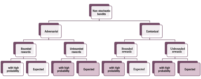
(a)

Figure 4: The framework of regret analysis in non-stochastic bandits.

As we see in Figure 4, the domain of regret analyses for non-stochastic regret bounds falls into 8 sub-categories by taking all the possible combinations of $A$ and $B$ and $C$, where $A=\{Contextual,Adversarial\},B=\{Bounded\,rewards,Unbounded\,rewards\},C=\{High\,probability\,bound,Expected\,bound\}$. The colored boxes in the leaf nodes correspond to the results in this paper and the remaining boxes are already covered by the existing literature. For contextual bandits, establishing a high probability regret bound is non-trivial even for bounded rewards since regret in a contextual setting significantly differs from the one in the adversarial setting. To this end, we propose a brand new algorithm EXP4.P that incorporates EXP3.P in adversarial MAB with EXP4. The analysis for regret of EXP4.P in unbounded cases is quite general and can be extended to EXP3.P without too much effort.

To conclude, the theoretical analyses regarding the upper bound fill the gap between the regret bound in Auer et al. [2002b] and all others in Figure 4.

E.2 Lower Bounds

Table 1: Boundary for $T$ as a function of $\mu$

$\mu$	$10^{-5}$	$10^{-4}$	$10^{-3}$	$10^{-2}$	$10^{-1}$
Upper bound for $T$	25001	2501	251	26	3.5

In view of unbounded bandits, the previous lower bound in Auer et al. [2002b] does not hold since unboundedness apparently increases regret. The relationship between the lower bound and time horizon is listed in Table  1 to facilitate the understanding of the lower bound. More precisely, Table 1 provides the values of the relationship between $\mu$ and largest $T$ in the Gaussian case where the inferior arms are distributed based on standard normal and the superior arms have mean $\mu>0$ and variance 1. As we can observe in the table, the maximum of $T$ for the lower bound to hold changes with instances. A small $\mu$ means the lower bound on regret of order $T$ holds for larger $T$. For example, there is no way to attain regret lower than $T\cdot 10^{-4}/4$ for any $1\leq T\leq 2501$. The function decreases very quickly. This coincides with the intuition since it would be difficult to distinguish between the optimal arm and the non-optimal ones given their rewards are close. A lower bound for large $T$ remains open.

References

- Auer et al. [2002a] P. Auer, N. Cesa-Bianchi, and P. Fischer. Finite-time analysis of the multiarmed bandit problem. Machine learning, 47(2-3):235–256, 2002a.
- Auer et al. [2002b] P. Auer, N. Cesa-Bianchi, Y. Freund, and R. E. Schapire. The nonstochastic multiarmed bandit problem. SIAM Journal on Computing, 32(1):48–77, 2002b.
- Balcan [2011] M. F. Balcan. 8803 machine learning theory. http://cs.cmu.edu/~ninamf/ML11/lect1117.pdf, 2011.
- Bellemare et al. [2016] M. Bellemare, S. Srinivasan, G. Ostrovski, T. Schaul, D. Saxton, and R. Munos. Unifying count-based exploration and intrinsic motivation. In Advances in Neural Information Processing Systems, pages 1471–1479, 2016.
- Burda et al. [2018] Y. Burda, H. Edwards, A. Storkey, and O. Klimov. Exploration by random network distillation. In International Conference on Learning Representations, 2018.
- Chatterjee [2014] S. Chatterjee. Superconcentration and related topics, volume 15. Cham: Springer, 2014.
- Deng et al. [2009] J. Deng, W. Dong, R. Socher, L.-J. Li, K. Li, and L. Fei-Fei. Imagenet: a large-scale hierarchical image database. In 2009 IEEE conference on Computer Vision and Pattern Recognition, pages 248–255. IEEE, 2009.
- Devroye et al. [2018] L. Devroye, A. Mehrabian, and T. Reddad. The total variation distance between high-dimensional gaussians. arXiv preprint arXiv:1810.08693, 2018.
- Duchi [2009] J. Duchi. Probability bounds. http://ai.stanford.edu/~jduchi/projects/probability_bounds.pdf, 2009.
- Fox et al. [2018] L. Fox, L. Choshen, and Y. Loewenstein. Dora the explorer: directed outreaching reinforcement action-selection. In International Conference on Learning Representations, 2018.
- Grünewälder et al. [2010] S. Grünewälder, J. Y. Audibert, M. Opper, and J. Shawe-Taylor. Regret bounds for gaussian process bandit problems. In Proceedings of the Thirteenth International Conference on Artificial Intelligence and Statistics, pages 273–280, 2010.
- Krizhevsky et al. [2012] A. Krizhevsky, I. Sutskever, and G. E. Hinton. Imagenet classification with deep convolutional neural networks. In Advances in Neural Information Processing Systems, pages 1097–1105, 2012.
- Mnih et al. [2013] V. Mnih, K. Kavukcuoglu, D. Silver, A. Graves, I. Antonoglou, D. Wierstra, and M. Riedmiller. Playing atari with deep reinforcement learning. arXiv preprint arXiv:1312.5602, 2013.
- Mnih et al. [2015] V. Mnih, K. Kavukcuoglu, D. Silver, A. A. Rusu, J. Veness, M. G. Bellemare, A. Graves, M. Riedmiller, A. K. Fidjeland, G. Ostrovski, and S. Petersen. Human-level control through deep reinforcement learning. Nature, 518(7540):529–533, 2015.
- Osband et al. [2016] I. Osband, C. Blundell, A. Pritzel, and B. Van Roy. Deep exploration via bootstrapped DQN. In Advances in Neural Information Processing Systems, pages 4026–4034, 2016.
- Osband et al. [2018] I. Osband, J. Aslanides, and A. Cassirer. Randomized prior functions for deep reinforcement learning. In Advances in Neural Information Processing Systems, pages 8617–8629, 2018.
- Rivlin [2019] O. Rivlin. Mountaincar_dqn_rnd. https://github.com/orrivlin/MountainCar_DQN_RND, 2019.
- Schulman et al. [2017] J. Schulman, F. Wolski, P. Dhariwal, A. Radford, and O. Klimov. Proximal policy optimization algorithms. arXiv preprint arXiv:1707.06347, 2017.
- Srinivas et al. [2010] N. Srinivas, A. Krause, S. Kakade, and M. Seeger. Gaussian process optimization in the bandit setting: no regret and experimental design. In Proceedings of the 27th International Conference on Machine Learning, 2010.
- Stadie et al. [2015] B. C. Stadie, S. Levine, and P. Abbeel. Incentivizing exploration in reinforcement learning with deep predictive models. arXiv preprint arXiv:1507.00814, 2015.
- Strehl and Littman [2008] A. L. Strehl and M. L. Littman. An analysis of model-based interval estimation for Markov decision processes. Journal of Computer and System Sciences, 74(8):1309–1331, 2008.
- Tokic [2010] M. Tokic. Adaptive -greedy exploration in reinforcement learning based on value differences. In Annual Conference on Artificial Intelligence, pages 203–210. Springer, 2010.
- Xia et al. [2011] R. Xia, C. Zong, and S. Li. Ensemble of feature sets and classification algorithms for sentiment classification. Information Sciences, 181(6):1138–1152, 2011.
- Zuo [2020] S. Zuo. Near optimal adversarial attack on UCB bandits. arXiv preprint arXiv:2008.09312, 2020.