Stochastic Gradient Langevin Dynamics Algorithms with Adaptive Drifts

Abstract

Bayesian deep learning offers a principled way to address many issues concerning safety of artificial intelligence (AI), such as model uncertainty,model interpretability, and prediction bias. However, due to the lack of efficient Monte Carlo algorithms for sampling from the posterior of deep neural networks (DNNs), Bayesian deep learning has not yet powered our AI system. We propose a class of adaptive stochastic gradient Markov chain Monte Carlo (SGMCMC) algorithms, where the drift function is biased to enhance escape from saddle points and the bias is adaptively adjusted according to the gradient of past samples. We establish the convergence of the proposed algorithms under mild conditions, and demonstrate via numerical examples that the proposed algorithms can significantly outperform the existing SGMCMC algorithms, such as stochastic gradient Langevin dynamics (SGLD), stochastic gradient Hamiltonian Monte Carlo (SGHMC) and preconditioned SGLD, in both simulation and optimization tasks.

Keywords: Adaptive MCMC, Adam, Bayesian Deep Learning, Momentum, Stochastic Gradient MCMC

1 Introduction

During the past decade, deep learning has been the engine powering many successes of artificial intelligence (AI). However, the deep neural network (DNN), as the basic model of deep learning, still suffers from some fundamental issues, such as model uncertainty, model interpretability, and prediction bias, which pose a high risk on the safety of AI. In particular, the standard optimization algorithms such as stochastic gradient descent (SGD) produce only a point estimate for the DNN, where model uncertainty is completely ignored. The machine prediction/decision is blindly taken as accurate and precise, with which the automated system might become life-threatening to humans if used in real-life settings. The universal approximation ability of the DNN enables it to learn powerful representations that map high-dimensional features to an array of outputs. However, the representation is less interpretable, from which important features that govern the function of the system are hard to be identified, causing serious issues in human-machine trust. In addition, the DNN often contains an excessively large number of parameters. As a result, the training data tend to be over-fitted and the prediction tends to be biased.

As advocated by many researchers, see e.g. Kendall and Gal (2017) and Chen (2018), Bayesian deep learning offers a principled way to address above issues. Under the Bayesian framework, a sparse DNN can be learned by sampling from the posterior distribution formulated with an appropriate prior distribution, see e.g. Liang et al. (2018) and Polson and Rockova (2018). For the sparse DNN, interpretability of the structure and consistency of the prediction can be established under mild conditions, and model uncertainty can be quantified based on the posterior samples, see e.g. Liang et al. (2018). However, due to the lack of efficient Monte Carlo algorithms for sampling from the posterior of DNNs, Bayesian deep learning has not yet powered our AI systems.

Toward the goal of efficient Bayesian deep learning, a variety of stochastic gradient Markov chain Monte Carlo (SGMCMC) algorithms have been proposed in the literature, including stochastic gradient Langevin dynamics (SGLD) (Welling and Teh, 2011), stochastic gradient Hamiltonian Monte Carlo (SGHMC) (Chen et al., 2014), and their variants. One merit of the SGMCMC algorithms is that they are scalable, requiring at each iteration only the gradient on a mini-batch of data as in the SGD algorithm. Unfortunately, as pointed out in Dauphin et al. (2014), DNNs often exhibit pathological curvature and saddle points, rendering the first-order gradient based algorithms, such as SGLD, inefficient. To accelerate convergence, the second-order gradient algorithms, such as stochastic gradient Riemannian Langevin dynamics (SGRLD)(Ahn et al., 2012; Girolami and Calderhead, 2011; Patterson and Teh, 2013) and stochastic gradient Riemannian Hamiltonian Monte Carlo (SGRHMC) (Ma et al., 2015), have been developed. With the use of the Fisher information matrix of the target distribution, these algorithms rescale the stochastic gradient noise to be isotropic near stationary points, which helps escape saddle points faster. However, calculation of the Fisher information matrix can be time consuming, which makes these algorithms lack scalability necessary for learning large DNNs. Instead of using the exact Fisher information matrix, preconditioned SGLD (pSGLD) (Li et al., 2016) approximates it by a diagonal matrix adaptively updated with the current gradient information.

Ma et al. (2015) provides a general framework for the existing SGMCMC algorithms (see Section 2), where the stochastic gradient of the energy function (i.e., the negative log-target distribution) is restricted to be unbiased. However, this restriction is unnecessary. As shown in the recent work, see e.g., Dalalyan and Karagulyan (2017), Song et al. (2020), and Bhatia et al. (2019), the stochastic gradient of the energy function can be biased as long as its mean squared error can be upper bounded by an appropriate function of $\theta_{t}$, the current sample of the stochastic gradient Markov chain. On the other hand, a variety of adaptive SGD algorithms, such as momentum (Qian, 1999), Adagrad (Duchi et al., 2011), RMSprop (Tieleman and Hinton, 2012), and Adam (Kingma and Ba, 2014), have been proposed in the recent literature for dealing with the saddle point issue encountered in deep learning. These algorithms adjust the moving direction at each iteration according to the current gradient as well as the past ones. It was shown in Staib et al. (2019) that, compared to SGD, these algorithms escape saddle points faster and can converge faster overall to the second-order stationary points.

Motivated by the two observations above, we propose a class of adaptive SGLD algorithms, where a bias term is included in the drift function to enhance escape from saddle points and accelerate the convergence in the presence of pathological curvatures. The bias term can be adaptively adjusted based on the path of the sampler. In particular, we propose to adjust the bias term based on the past gradients in the flavor of adaptive SGD algorithms (Ruder, 2016). We establish the convergence of the proposed adaptive SGLD algorithms under mild conditions, and demonstrate via numerical examples that the adaptive SGLD algorithms can significantly outperform the existing SGMCMC algorithms, such as SGLD, SGHMC and pSGLD.

2 A Brief Review of Existing SGMCMC Algorithms

Let ${X}_{N}=(X_{1},X_{2},\ldots,X_{N})$ denote a set of $N$ independent and identically distributed samples drawn from the distribution $f(x|\theta)$, where $N$ is the sample size and $\theta$ is the vector of parameters. Let $p({X}_{N}|\theta)=\prod_{i=1}^{N}f(X_{i}|\theta)$ denote the likelihood function, let $\pi(\theta)$ denote the prior distribution of $\theta$, and let $U(\theta)=-\log p({X}_{N}|\theta)-\log\pi(\theta)$ denote the energy function of the posterior distribution. If $\theta$ has a fixed dimension and $U(\theta)$ is differentiable with respect to $\theta$, then the SGLD algorithm can be used to simulate from the posterior, which iterates by

$$\theta_{t+1}=\theta_{t}-\epsilon_{t+1}\nabla_{\theta}\tilde{U}(\theta_{t})+\sqrt{2\epsilon_{t+1}\tau}\eta_{t+1},\ \ \eta_{t+1}\sim N(0,I_{d}),$$

where $d$ is the dimension of $\theta$, $I_{d}$ is an $d\times d$-identity matrix, $\epsilon_{t+1}$ is the learning rate, $\tau$ is the temperature, and $\nabla_{\theta}\tilde{U}(\theta)$ denotes an estimate of $\nabla_{\theta}U(\theta)$ based on a mini-batch of data. The learning rate can be kept as a constant or decreasing with iterations. For the former, the convergence of the algorithm was studied in Sato and Nakagawa (2014) and Dalalyan and Karagulyan (2017). For the latter, the convergence of the algorithm was studied in Teh et al. (2016).

The SGLD algorithm has been extended in different ways. As mentioned previously, each of its existing variants can be formulated as a special case of a general SGMCMC algorithm given in Ma et al. (2015). Let $\xi$ denote an augmented state, which may include some auxiliary components. For example, SGHMC augments the state to $\xi=(\theta,v)$ by including an auxiliary velocity component denoted by $v$. Then the general SGMCMC algorithm is given by

$$\theta_{t+1}=\theta_{t}-\epsilon_{t+1}[D(\xi)+Q(\xi)]\nabla_{\xi}\tilde{H}(\xi)+\Gamma(\xi)+\sqrt{2\epsilon_{t+1}\tau}Z_{t+1},$$

where $Z_{t+1}\sim N(0,D(\xi_{t}))$, $H(\xi)$ is the energy function of the augmented system, $\nabla_{\xi}\tilde{H}(\xi)$ denotes an unbiased estimate of $\nabla_{\xi}H(\xi)$, $D(\xi)$ is a positive semi-definite diffusion matrix, $Q(\xi)$ is a skew-symmetric curl matrix, and $\Gamma_{i}(\xi)=\sum_{j=1}^{d}\frac{\partial}{\partial\xi_{j}}(D_{ij}(\xi)+Q_{ij}(\xi))$. The diffusion $D(\xi)$ and curl $Q(\xi)$ matrices can take various forms and the choice of the matrices will affect the rate of convergence of the sampler. For example, for the SGHMC algorithm, we have $H(\xi)=U(\theta)+\frac{1}{2}v^{T}v$, $D(\xi)=\begin{pmatrix}0&0\\ 0&C\end{pmatrix}$ for some positive semi-definite matrix $C$, and $Q(\xi)=\begin{pmatrix}0&-I\\ I&0\end{pmatrix}$. For the SGRLD algorithm, we have $\xi=\theta$, $H(\xi)=U(\theta)$, $D(\xi)=G(\theta)^{-1}$, $Q(\xi)=0$, where $G(\theta)$ is the Fisher information matrix of the posterior distribution. By rescaling the parameter updates according to geometry information of the manifold, SGRLD generally converges faster than SGLD. However, calculating the Fisher information matrix and its inverse can be time consuming when the dimension of $\theta$ is high and the total sample size $N$ is large. To address this issue, pSGLD approximates $G(\theta)$ using a diagonal matrix and sequentially updates the approximator using the current gradient information. To be more precise, it is given by

$$\begin{split}G(\theta_{t+1})&={\rm diag}(1\oslash(\lambda\bf{1}+\sqrt{V(\theta_{t+1})})),\\ V(\theta_{t+1})&=\beta V(\theta_{t})+(1-\beta)\nabla_{\theta}\tilde{U}(\theta_{t})\odot\nabla_{\theta}\tilde{U}(\theta_{t}),\end{split}$$

where $\lambda$ denotes a small constant, $\odot$ and $\oslash$ represent element-wise vector product and division, respectively.

3 Stochastic Gradient Langevin Dynamics with Adaptive Drifts

Motivated by the observations that the stochastic gradient $\nabla_{\theta}\tilde{U}(\theta)$ used in SGLD is not necessarily unbiased and that the past gradients can be used to enhance escape from saddle points for SGD, we propose a class of adaptive SGLD algorithms, where the past gradients are used to accelerate the convergence of the sampler by forming a bias to the drift at each iteration. A general form of the adaptive SGLD algorithm is given by

$$\theta_{t+1}=\theta_{t}-\epsilon_{t+1}(\nabla_{\theta}\tilde{U}(\theta_{t})+aA_{t})+\sqrt{2\epsilon_{t+1}\tau}\eta_{t+1},$$ (1)

where $A_{t}$ is the adaptive bias term, $a$ is called the bias factor, and $\eta_{t+1}\sim N(0,I_{d})$. Two adaptive SGLD algorithms are given in what follows. In the first algorithm, the bias term is constructed based on the momentum algorithm (Qian, 1999); and in the second algorithm, the bias term is constructed based on the Adam algorithm (Kingma and Ba, 2014).

3.1 Momentum SGLD

It is known that SGD has trouble in navigating ravines, i.e., the regions where the energy surface curves much more steep in one dimension than in another, which are common around local energy minima (Ruder, 2016; Sutton, 1986). In this scenario, SGD oscillates across the slopes of the ravine while making hesitant progress towards the local energy minima. To accelerate SGD in the relevant direction and dampen oscillations, the momentum algorithm (Qian, 1999) updates the moving direction at each iteration by adding a fraction of the moving direction of the past iteration, the so-called momentum term, to the current gradient. By accumulation, the momentum term increases updates for the dimensions whose gradients pointing in the same directions and reduces updates for the dimensions whose gradients change directions. As a result, the oscillation is reduced and the convergence is accelerated.

Algorithm 1 MSGLD

  Input: Data $\{x_{i}\}_{i=1}^{N}$, subsample size $n$, smoothing factor $0<\beta_{1}<1$, bias factor $a$, temperature $\tau$, and learning rate $\epsilon$;

  Initialization: $\theta_{0}$ from an appropriate distribution, and $m_{0}=0$.

  for $i=1,2,\dots,$ do

     Draw a mini-batch of data $\{x_{j}^{*}\}_{j=1}^{n}$, and calculate

     $\theta_{t+1}=\theta_{t}-\epsilon(\nabla\tilde{U}(\theta_{t})+am_{t})+e_{t+1}$,

     $m_{t}=\beta_{1}m_{t-1}+(1-\beta_{1})\nabla\tilde{U}(\theta_{t-1})$, where $e_{t+1}\sim N(0,2\tau\epsilon I_{d})$, and $d$ is the dimension of $\theta$.

  end for

As an analogy of the momentum algorithm in stochastic optimization, we propose the so-called momentum SGLD (MSGLD) algorithm, where the momentum is calculated as an exponentially decaying average of past stochastic gradients and added as a bias term to the drift of SGLD. The resulting algorithm is depicted in Algorithm 1, where a constant learning rate $\epsilon$ is considered for simplicity. However, as mentioned in the Appendix, the algorithm also works for the case that the learning rate decays with iterations. The convergence of the algorithm is established in Theorem 3.1, whose proof is given in the Appendix.

Theorem 3.1 (Ergodicity of MSGLD)

Suppose the conditions (A.1)-(A.5) hold (given in Appendix), $\beta_{1}\in(0,1]$ is a constant, and the learning rate $\epsilon$ is sufficiently small. Then for any smooth function $\phi(\theta)$,

$$\frac{1}{L}\sum_{k=1}^{L}\phi(\theta_{k})-\int_{\Theta}\phi(\theta)\pi_{*}(\theta)d\theta\stackrel{{\scriptstyle p}}{{\to}}0,\quad\mbox{as $L\to\infty$},$$

where $\pi_{*}$ denotes the posterior distribution of $\theta$, and $\stackrel{{\scriptstyle p}}{{\to}}$ denotes convergence in probability.

Algorithm 1 contains a few parameters, including the subsample size $n$, smoothing factor $\beta_{1}$, bias factor $a$, temperature $\tau$, and learning rate $\epsilon$. Among these parameters, $n$, $\tau$ and $\epsilon$ are shared with SGLD and can be set as in SGLD. Refer to Nagapetyan et al. (2017) and Nemeth and Fearnhead (2019) for more discussions on their settings. The smoothing factor $\beta_{1}$ is a constant, which is typically set to 0.9. The bias factor $a$ is also a constant, which is typically set to 1 or a slightly large value.

3.2 Adam SGLD

The Adam algorithm (Kingma and Ba, 2014) has been widely used in deep learning, which typically converges much faster than SGD. Recently, Staib et al. (2019) showed that Adam can be viewed as a preconditioned SGD algorithm, where the preconditioner is estimated in an on-line manner and it helps escape saddle points by rescaling the stochastic gradient noise to be isotropic near stationary points.

Algorithm 2 ASGLD

  Input: Data $\{x_{i}\}_{i=1}^{N}$, subsample size $n$, smoothing factors $\beta_{1}$ and $\beta_{2}$, bias factor $a$, temperature $\tau$, and learning rate $\epsilon$;

  Initialization: $\theta_{0}$ from appropriate distribution, $m_{0}=0$ and $V_{0}=0$;

  for $i=1,2,\dots,$ do

     Draw a mini-batch of data $\{x_{j}^{*}\}_{j=1}^{n}$, and calculate

     $\theta_{t+1}=\theta_{t}-\epsilon(\nabla\tilde{U}(\theta_{t})+am_{t}\oslash\sqrt{V_{t}+\lambda{\bf 1}})+e_{t+1},$

     $m_{t}=\beta_{1}m_{t-1}+(1-\beta_{1})\nabla\tilde{U}(\theta_{t-1})$,

     $V_{t}=\beta_{2}V_{t-1}+(1-\beta_{2})\nabla\tilde{U}(\theta_{t-1})\odot\nabla\tilde{U}(\theta_{t-1})$, where $\lambda$ is a small constant added to avoid zero-divisors, $e_{t+1}\sim N(0,2\tau\epsilon I_{d})$, and $d$ is the dimension of $\theta$.

  end for

Motivated by this result, we propose the so-called Adam SGLD (ASGLD) algorithm. Ideally, we would construct the adaptive bias term as follows:

$$\begin{split}m_{t}&=\beta_{1}m_{t-1}+(1-\beta_{1})\nabla\tilde{U}(\theta_{t-1}),\\ \tilde{V}_{t}&=\beta_{2}\tilde{V}_{t-1}+(1-\beta_{2})\tilde{U}(\theta_{t-1})\tilde{U}(\theta_{t-1})^{T},\\ \tilde{A}_{t}&=\tilde{V}_{t}^{-1/2}m_{t},\end{split}$$ (2)

where $\beta_{1}$ and $\beta_{2}$ are smoothing factors for the first and second moments of stochastic gradients, respectively. Since $\tilde{V}_{t}$ can be viewed as an approximator of the true second moment matrix $E(\nabla_{\theta}\tilde{U}(\theta_{t-1})\nabla_{\theta}\tilde{U}(\theta_{t-1})^{T})$ at iteration $t-1$, $\tilde{A}_{t}$ can viewed as the rescaled momentum which is isotropic near stationary points. If the bias factor $a$ is chosen appropriately, ASGLD is expected to converge very fast. In particular, the bias term may guide the sampler to converge to a global optimal region quickly, similar to Adam in optimization. However, when the dimension of $\theta$ is high, calculation of $\tilde{V}_{t}$ and $\tilde{V}_{t}^{-1/2}$ can be time consuming. To accelerate computation, we propose to approximate $\tilde{V}_{t}$ using a diagonal matrix as in pSGLD. This leads to Algorithm 2. The convergence of the algorithm is established in Theorem 3.2, whose proof is given in the Appendix.

Theorem 3.2 (Ergodicity of ASGLD)

Suppose the conditions (A.1)-(A.5) hold (given in Appendix), $\beta_{1}^{2}<\beta_{2}$ are two constants between 0 and 1, and the learning rate $\epsilon$ is sufficiently small. Then for any smooth function $\phi(\theta)$,

$$\frac{1}{L}\sum_{k=1}^{L}\phi(\theta_{k})-\int_{\Theta}\phi(\theta)\pi_{*}(\theta)d\theta\stackrel{{\scriptstyle p}}{{\to}}0,\quad\mbox{as $L\to\infty$},$$

where $\pi_{*}$ denotes the posterior distribution of $\theta$, and $\stackrel{{\scriptstyle p}}{{\to}}$ denotes convergence in probability.

Compared to Algorithm 1, ASGLD contains one more parameter, $\beta_{2}$, which works as the smoothing factor for the second moment term and is suggested to take a value of 0.999 in this paper.

3.3 Other Adaptive SGLD Algorithms

In addition to the Momentum and Adam algorithms, other optimization algorithms, such as AdaMax (Kingma and Ba, 2014) and Adadelta (Zeiler, 2012), can also be incorporated into SGLD to accelerate its convergence. Other than the bias term, the past gradients can also be used to construct an adaptive preconditioner matrix in a similar way to pSGLD. Moreover, the adaptive bias and adaptive preconditioner matrix can be used together to accelerate the convergence of SGLD.

4 Illustrative Examples

Before applying the adaptive SGLD algorithms to DNN models, we first illustrate their performance on three low-dimensional examples. The first example is a multivariate Gaussian distribution with high correlation values. The second example is a multi-modal distribution, which mimics the scenario with multiple local energy minima. The third example is more complicated, which mimics the scenario with long narrow ravines.

4.1 A Gaussian distribution with high correlation values

Suppose that we are interested in drawing samples from $\pi(\theta)$, a Gaussian distribution with the mean zero and the covariance matrix $\Sigma=\begin{pmatrix}1&0.9\\ 0.9&1\end{pmatrix}$. For this example, we have $\nabla_{\theta}U(\theta)=\Sigma^{-1}\theta$, and set $\nabla\tilde{U}(\theta)=\nabla U(\theta)+e$ in simulations, where $\theta=(\theta_{1},\theta_{2})^{T}\in\mathbb{R}^{2}$ and $e\sim N(0,I_{2})$. For ASGLD, we set $\tau=1$, $a=0.1$, $\epsilon=0.1$, $\beta_{1}=0.9$ and $\beta_{2}=0.999$. For MSGLD, we set $\tau=1$, $a=0.01$, $\beta_{1}=0.9$ and $\epsilon=0.1$. For comparison, SGLD was also run for this example with the same learning rate $\epsilon=0.1$. Figure 1 shows that both ASGLD and MSGLD work well for this example, where the left panel shows that they can produce the same accurate estimate as SGLD for the covariance matrix as the number of iterations becomes large.

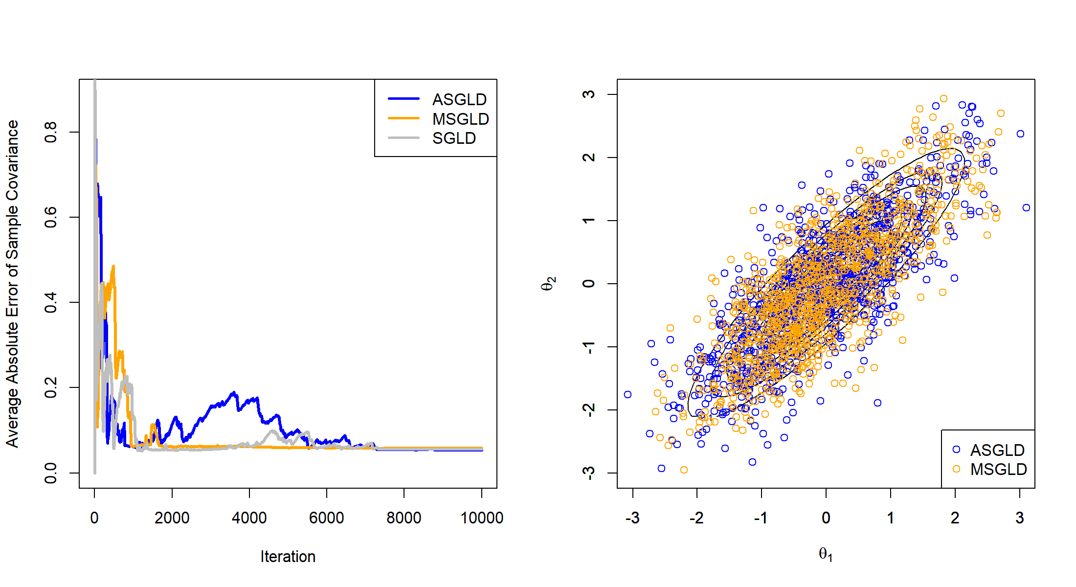
Figure 1: Performance of adaptive SGLD algorithms: (left) average absolute errors of the sample covariance matrix produced by SGLD, ASGLD and MSGLD along with iterations, and (right) scatter plots of the samples generated by ASGLD and MSGLD during their first 1000 iterations.

4.2 A multi-modal distribution

The target distribution is a 2-dimensional 5-component mixture Gaussian distribution, whose density function is given by $\pi(\theta)=\sum_{i=1}^{5}\frac{1}{10\pi}\exp(-\|\theta-\mu_{i}\|^{2})$, where $\mu_{1}=(-3,-3)^{T},\mu_{2}=(-3,0)^{T},\mu_{3}=(0,0)^{T},\mu_{4}=(3,0)^{T},\mu_{5}=(3,3)^{T}$. For this example, we considered the natural gradient variational inference (NGVI) algorithm (Lin et al., 2019), which is known to converge very fast in the variational inference field, as the baseline algorithm for comparison.

For adaptive SGLD method, both ASGLD and MSGLD were applied to this example. We set $\nabla_{\theta}\tilde{U}(\theta)=\nabla U(\theta)+e$, where $e\sim N(0,I_{2})$ and $U(\theta)=-\log\pi(\theta)$. For a fair comparison, each algorithm was run in 6.0 CPU minutes. The numerical results were summarized in Figure 2, which shows the contour of the energy function and its estimates by NGVI, MSGLD and ASGLD. The plots indicate that MSGLD and ASGLD are better at exploring the multi-modal distributions than NGVI.

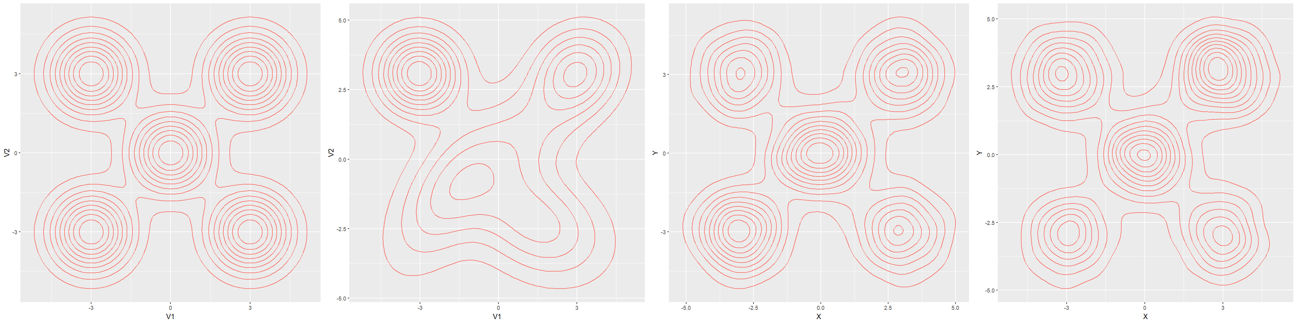
Figure 2: Contour plots of the true energy function (left) and its estimates by NGVI (middle left), MSGLD (middle right), and ASGLD (right).

4.3 A distribution with long narrow energy ravines

Consider a nonlinear regression

$$y=f_{\theta}(x)+\epsilon,\quad\epsilon\sim N(0,1),$$

where $x\sim Unif[-2,4]$, $\theta=(\theta_{1},\theta_{2})^{T}\in\mathbb{R}^{2}$, and $f_{\theta}(x)=(x-1)^{2}+2\sin(\theta_{1}x)+\frac{1}{30}\theta_{1}+\cos(\theta_{2}x-1)-\frac{1}{20}\theta_{2}$. As $\theta$ increases, the function $f_{\theta}(x)$ fluctuates more severely. Figure 3(a) depicts the regression, where we set $\theta_{1}=20$ and $\theta_{2}=10$. Since the random error $\epsilon$ is relatively large compared to the local fluctuation of $f_{\theta}(x)$, i.e., $2\sin(\theta_{1}x)+\frac{1}{30}\theta_{1}+\cos(\theta_{2}x-1)-\frac{1}{20}\theta_{2}$, identification of the exact values of $(\theta_{1},\theta_{2})$ can be very hard, especially when the subsample size $n$ is small.

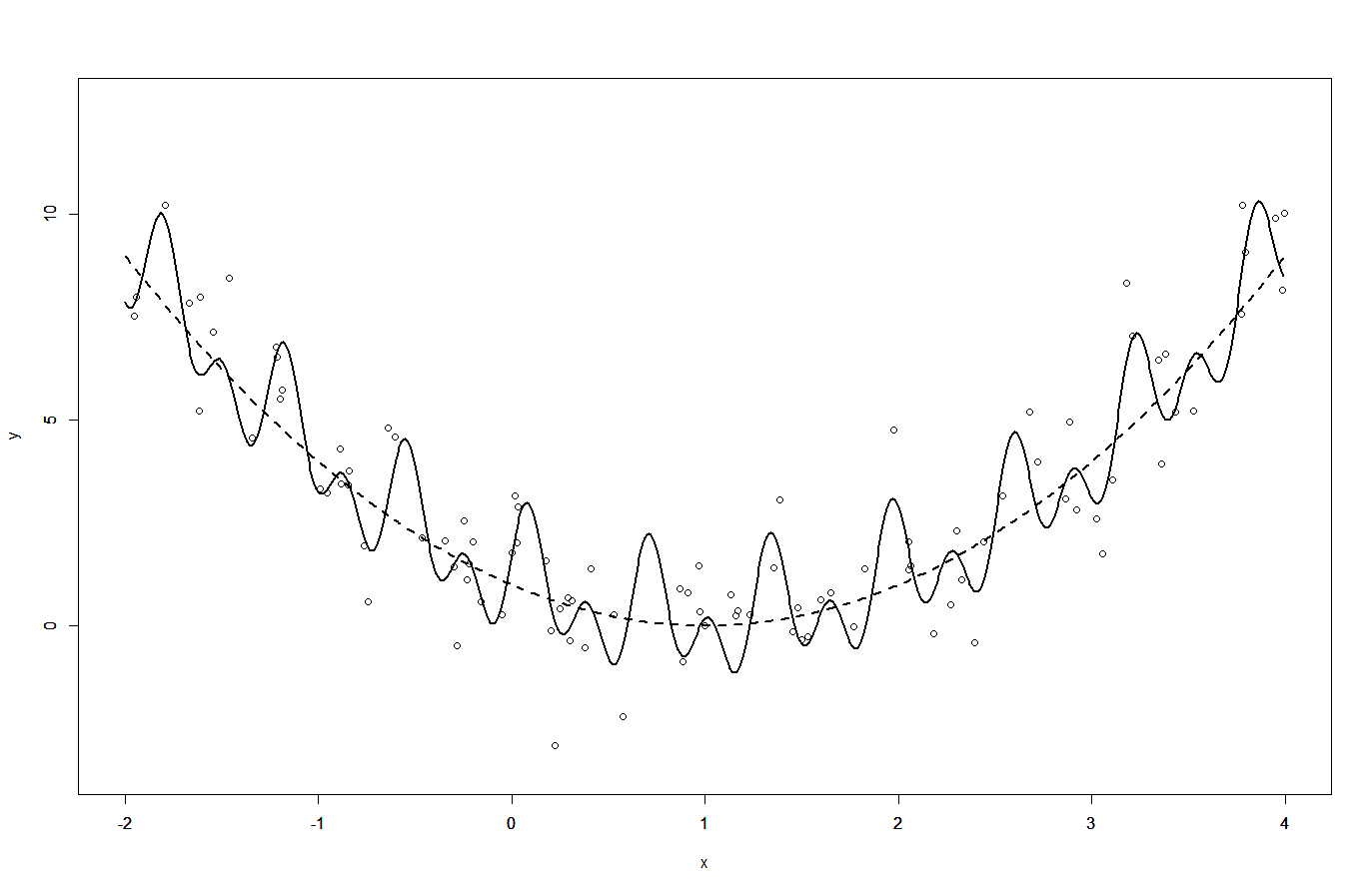
(a)

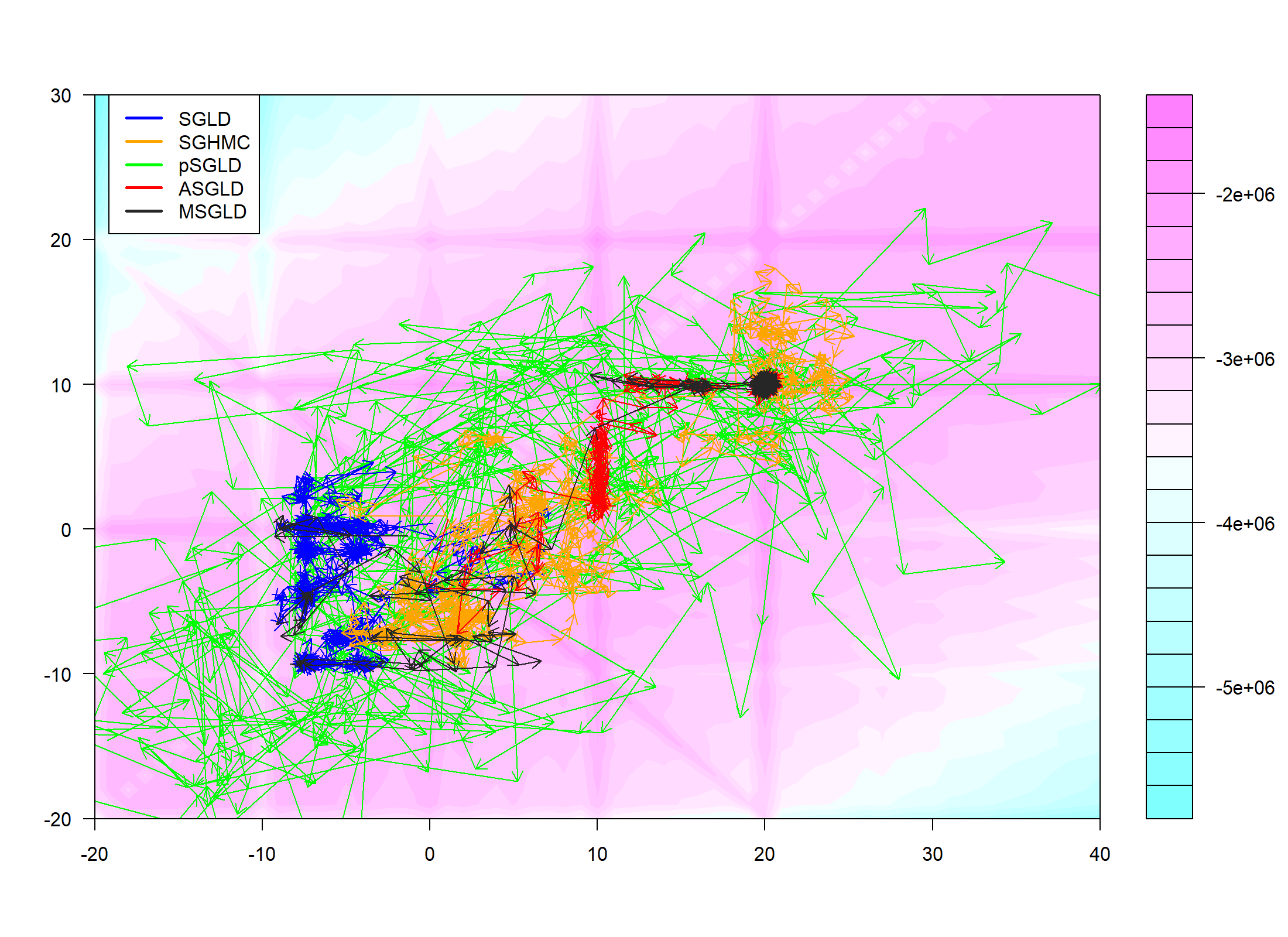
(b)

Figure 3: (a) The dashed line is for the global pattern $(x-1)^{2}$ and the solid line is for the regression function $f_{\theta}(x)$, where $\theta_{1}=20$ and $\theta_{2}=10$. The points represent 100 random samples from the regression. (b) Contour plot of the energy function for one dataset and the sample paths produced by SGLD, SGHMC, pSGLD, ASGLD and MSGLD in a run, where the sample paths have been thinned by a factor of 50 for readability of the plot.

From this regression, we simulated 5 datasets with $(\theta_{1},\theta_{2})=(20,10)$ independently. Each dataset consists of 10,000 samples. To conduct Bayesian analysis for the problem, we set the prior distribution: $\theta_{1}\sim N(0,1)$ and $\theta_{2}\sim N(0,1)$, which are a priori independent. This choice of the prior distribution makes the problem even harder, which discourages the convergence of the posterior simulation to the true value of $\theta$. Instead, it encourages to estimate $f_{\theta}(x)$ by the global pattern $(x-1)^{2}$.

Both ASGLD and MSGLD were run for each of the 5 datasets. Each run consisted of 30,000 iterations, where the first 10,000 iterations were discarded for the burn-in process and the samples generated from the remaining 20,000 iterations were averaged as the Bayesian estimate of $\theta$. In the simulations, we set the subsample size $n=100$. The settings of other parameters are given in the Appendix. Table 1 shows the Bayesian estimates of $\theta$ produced by the two algorithms in each of the five runs. The MSGLD estimate converged to the true value in all five runs, while the ASGLD estimates converged to the true value in four of five runs. For comparison, SGLD, SGHMC and pSGLD were also applied to this example with the settings given in the Appendix. As implied by Table 1, all the three algorithms essentially failed for this example: none of their estimates converged to the true value!

Table 1: Bayesian estimates of $\theta$ produced by different algorithms for the long narrow energy ravines example in five independent runs, where the true value of $\theta$ is (20,10).

Method	$\theta$	1	2	3	4	5
	$\theta_{1}$	-5.79	-6.59	17.43	0.99	-3.01
SGLD	$\theta_{2}$	-2.42	-1.76	9.02	-1.36	-4.74
	$\theta_{1}$	9.22	14.73	23.19	11.39	-4.22
SGHMC	$\theta_{2}$	1.27	6.23	11.03	2.65	-2.25
	$\theta_{1}$	1.27	-19.77	16.52	5.14	-9.08
pSGLD	$\theta_{2}$	-2.22	-15.44	8.17	0.65	3.75
	$\theta_{1}$	19.75	15.34	19.99	19.01	19.98
ASGLD	$\theta_{2}$	9.99	9.29	9.92	9.66	9.99
	$\theta_{1}$	20.01	20.07	19.99	20.00	19.99
MSGLD	$\theta_{2}$	9.99	10.00	9.99	9.99	9.99

For a further exploration, Figure 3(b) shows the contour plot of the energy function for one dataset as well as the sample paths produced by SGLD, SGHMC, pSGLD, ASGLD and MSGLD for the dataset. As shown by the contour plot, the energy landscape contains multiple long narrow ravines, which make the existing SGMCMC algorithms essentially fail. However, due to the use of momentum information, ASGLD and MSGLD work extremely well for this example. As indicated by their sample paths, they can move along narrow ravines, and converge to the true value of $\theta$ very quickly. It is interesting to point out that pSGLD does not work well for this example, although it has used the past gradients in constructing the preconditioned matrix. A possible reason for this failure is that it only approximates the preconditioned matrix by a diagonal matrix and missed the correlation between different components of $\theta$.

5 DNN Applications

5.1 Landsat Data

The dataset is available at the UCI Machine Learning Repository, which consists of 4435 training instances and 2000 testing instances. Each instance consists of 36 attributes which represent features of the earth surface images taken from a satellite. The training instances consist of 6 classes, and the goal of this study is to learn a classifier for the earth surface images.

We modeled this dataset by a fully connected DNN with structure 36-30-30-6 and Relu as the activation function. Let $\theta$ denote the vector of all parameters (i.e., connection weights) of the DNN. We let $\theta$ be subject to a Gaussian prior distribution: $\theta\sim N(0,I_{d})$, where $d$ is the dimension of $\theta$. The SGLD, SGHMC, pSGLD, ASGLD and MSGLD algorithms were all applied to simulate from the posterior of the DNN. Each algorithm was run for 3,000 epochs with the subsample size $n=50$ and a decaying learning rate

$$\epsilon_{k}=\epsilon_{0}\gamma^{\lfloor k/L\rfloor},$$ (3)

where $k$ indexes epochs, the initial learning rate $\epsilon_{0}=0.1$, $\gamma=0.5$, the step size $L=300$, and $\lfloor z\rfloor$ denotes the maximum integer less than $z$. For the purpose of optimization, the temperature was set to $\tau=0.01$. The settings for the specific parameters of each algorithm were given in the Appendix.

Each algorithm was run for five times for the example. In each run, the training and test classification accuracy were calculated by averaging over the last $200$ samples, which were collected from the last 100,000 iterations with a thinning factor of $500$. For each algorithm, Table 2 reports the mean classification accuracy, for both training and test, averaged over five runs and its standard deviation. The results indicate that MSGLD has significantly outperforms other algorithms in both training and test for this example. While ASGLD performs similarly to pSGLD for this example.

Table 2: Training and test classification accuracy produced by different SGMCMC algorithms for the Landsat data, where the accuracy and its standard error were calculated based on $5$ independent runs.

Method	Training Accuracy	Test Accuracy
SGLD	93.163$\pm$0.085	90.225$\pm$0.153
pSGLD	93.857$\pm$ 0.125	90.712$\pm$0.090
SGHMC	94.015$\pm$0.117	90.848$\pm$0.089
ASGLD	93.827$\pm$0.087	90.794$\pm$0.087
MSGLD	94.910 $\pm$0.105	91.247 $\pm$0.141

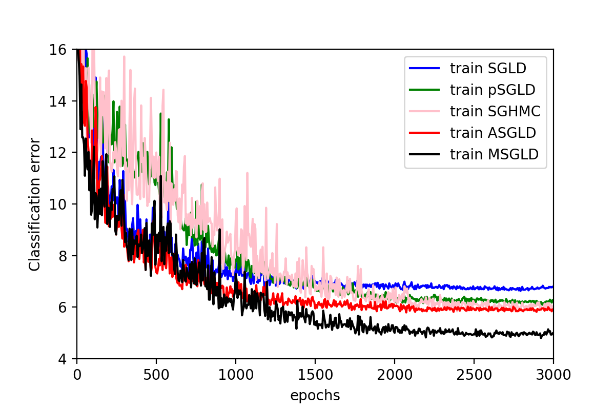
(a)

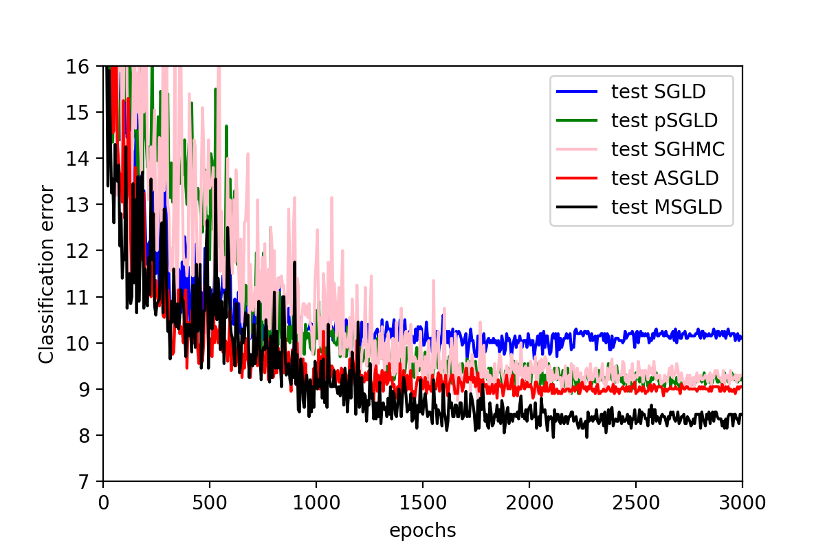
(b)

Figure 4: (a) Training classification errors produced by different SGMCMC algorithms for the Landsat data example. (b) Test classification errors produced by different SGMCMC algorithms for the Landsat data example.

Finally, we note that for this example, the SGMCMC algorithms have been run excessively long. Figure 4(a) and Figure 4(b) show, respectively, the training and test classification errors produced by SGLD, pSGLD, SGHMC, ASGLD and MSGLD along with iterations. It indicates again that MSGLD significantly outperforms other algorithms in both training and test.

5.2 MNIST data

The MNIST is a benchmark dataset of computer vision, which consists of 60,000 training instances and 10,000 test instances. Each instance is an image consisting of $28\times 28$ attributes and representing a hand-written number of 0 to 9. For this data set, we tested whether ASGLD or MSGLD can be used to train sparse DNNs. For this purpose, we considered a mixture Gaussian prior for each of the connection weights:

$$\pi(\theta_{k})\sim\lambda_{k}N(0,\sigma_{1,k}^{2})+(1-\lambda_{k})N(0,\sigma_{0,k}^{2}),$$ (4)

where $k$ is the index of hidden layers, and $\sigma_{0,k}$ is a relatively very small value compared to $\sigma_{1,k}$. In this paper, we set $\lambda_{k}=10^{-7},\ \sigma_{1,k}^{2}=0.02,\ \sigma_{0,k}^{2}=1\times 10^{-5}$ for all $k$.

We trained a DNN with structure 784-800-800-10 using ASGLD and MSGLD for 250 epochs with subsample size $100$. For the first $100$ epochs, the DNN was trained as usual, i.e., with a Gaussian prior $N(0,I_{d})$ imposed on each connection weight. Then the DNN was trained for 150 epochs with the prior (4). The settings for the other parameters of the algorithms were given in the Appendix. Each algorithm was run for 3 times. In each run, the training and prediction accuracy were calculated by averaging, respectively, the fitting and prediction results over the iterations of the last 5 epochs. The numerical results were summarized in Table 3, where “Sparse ratio” is calculated as the percentage of the learned connection weights satisfying the inequality $|\theta_{k}|\geq\sqrt{\log(\frac{1-\lambda_{k}}{\lambda_{k}}\frac{\sigma_{1k}}{\sigma_{0k}})\frac{2\sigma_{0k}^{2}\sigma_{1k}^{2}}{\sigma_{1k}^{2}-\sigma_{0k}^{2}}}$. The threshold is determined by solving the probability inequality $P\{\theta_{k}\sim N(0,\sigma_{0,k}^{2})|\theta_{k}\}\leq P\{\theta_{k}\sim N(0,\sigma_{1,k}^{2})|\theta_{k}\}$.

Table 3: Comparison of different algorithms for training sparse DNNs for the MNIST data, where the reported results for each algorithm were averaged based on three independent runs.

Method	Training Accuracy	Test Accuracy	Sparsity Ratio
ASGLD	99.542$\pm$ 0.026	98.417$\pm$0.044	3.176$\pm$0.155
MSGLD	99.494$\pm$ 0.002	98.319 $\pm$0.019	3.369$\pm$0.063
ADAM	99.383$\pm$0.072	98.332$\pm$0.003	2.169$\pm$0.013

Adam is a well known DNN optimization method for MNIST data. For comparison, it was also applied to train the sparse DNN. Interestingly, ASGLD outperforms Adam in both training and prediction accuracy, although its resulting network is a little more dense than that by Adam.

5.3 CIFAR 10 and CIFAR 100

The CIFAR-10 and CIFAR-100 are also benchmark datasets of computer vision. CIFAR-10 consists of 50,000 training images and 10,000 test images, and the images were classified into 10 classes. The CIFAR-100 dataset consists of 50,000 training images and 10,000 test images, but the images were classified into 100 classes. We modeled both datasets using a ResNet-18He et al. (2015), and trained the model for 250 epochs using various optimization and SGMCMC algorithms, including SGD, Adam, SGLD, SGHMC, pSGLD, ASGLD and MSGLD with data augmentation techniques. The temperature $\tau$ was set to $1.0e-5$ for all SGMCMC methods. The subsample sample size was set to 100. For CIFAR-10, the learning rate was set as in (3) with $L=40$ and $\gamma=0.5$; and the weight prior was set to $N(0,\frac{1}{25}I_{d})$ for all SGMCMC algorithms. For CIFAR-100, the learning rate was set as in (3) with $L=90$ and $\gamma=0.1$; and the weight prior was set to $N(0,\frac{1}{25}I_{d})$ for SGLD, pSGLD, and SGHMC, and $N(0,\frac{1}{75}I_{d})$ for ASGLD and MSGLD. For SGD and Adam, we set the objective function as

$$-\frac{1}{n}\sum_{i=1}^{n}\log f(x_{i}|\theta)+\frac{1}{2}\lambda\|\theta\|^{2},$$ (5)

where $f(x_{i}|\theta)$ denotes the likelihood function of observation $i$, and $\lambda$ is the regularization parameter. For SGD we set $\lambda=5.0e-4$; and for Adam we set $\lambda=0$. For Adam, we have also tried the case $\lambda\neq 0$, but the results were inferior to those reported below.

For each dataset, each algorithm was run for 5 times. In each run, the training and test classification errors were calculated by averaging over the iterations of the last 5 epochs. Table 4 reported the mean training and test classification accuracy (averaged over 5 runs) of the Bayesian ResNet-18 for CIFAR-10 and CIFAR-100. The comparison indicates that MSGLD outperforms all other algorithms in test accuracy for the two datasets. In terms of training accuracy, ASGLD and MSGLD work more like the existing momentum-based algorithms such as ADAM and SGHMC, but tend to generalize better than them. This result has been very remarkable, as all algorithms were run with a small number of epochs; that is, the Monte Carlo algorithms are not necessarily slower than the stochastic optimization algorithms in deep learning.

Table 4: Mean training and test classification accuracy (averaged over 5 runs) of the Bayesian ResNet-18 for CIFAR-10 and CIFAR-100 data

	CIFAR-10			CIFAR-100
Method	Training	Test		Training	Test
SGD	99.721$\pm$0.058	92.896$\pm$0.141		98.211$\pm$0.208	72.274$\pm$0.145
ADAM	99.515$\pm$0.087	92.144$\pm$0.154		96.744$\pm$0.390	67.564$\pm$0.501
SGLD	99.713$\pm$0.034	92.908$\pm$0.114		97.650$\pm$0.131	71.908$\pm$0.149
pSGLD	97.209$\pm$0.465	89.398$\pm$0.379		99.034$\pm$0.101	69.234$\pm$0.162
SGHMC	99.152$\pm$0.060	93.470$\pm$0.073		96.92$\pm$0.091	73.112$\pm$0.139
ASGLD	99.738$\pm$0.052	93.018$\pm$0.187		96.938$\pm$0.268	73.252$\pm$0.681
MSGLD	99.702$\pm$0.066	93.512$\pm$0.081		96.801$\pm$0.150	73.670$\pm$0.144

6 Conclusion

This paper has proposed a class of adaptive SGMCMC algorithms by including a bias term to the drift of SGLD, where the bias term is allowed to be adaptively adjusted with past samples, past gradients, etc. The proposed algorithms have extended the framework of the existing SGMCMC algorithms to an adaptive one in a flavor of extending the Metropolis algorithm Metropolis et al. (1953) to the adaptive Metropolis algorithm (Haaro et al., 2001) in the history of MCMC. The numerical results indicate that the proposed algorithms have inherited many attractive properties, such as quick convergence in the scenarios with long narrow ravines or saddle points, from their counterpart optimization algorithms, while ensuring more extensive exploration of the sample space than the optimization algorithms due to their simulation nature. As a result, the proposed algorithms can significantly perform the existing optimization and SGMCMC algorithms in both simulation and optimization.

For the adaptive SGMCMC algorithms, different bias terms represent different strengths in escaping from local traps, saddle points, or long narrow ravines. In the future, we will consider to develop an adaptive SGMCMC algorithm with a complex bias term which has incorporated all the strengths in escaping from local traps, saddle points, long narrow ravines, etc. We will also consider to incorporate other advanced SGMCMC techniques into adaptive SGMCMC algorithms to further improve their performance. For example, cyclical SGMCMC (Zhang et al., 2019) proposed a cyclical step size schedule, where larger steps discover new modes, and smaller steps characterize each mode. This technique can be easily incorporated into adaptive SGLD algorithms to improve their convergence to the stationary distribution.

Appendix

Appendix A Proofs of Theorems 3.1 and 3.2

Considered a generalized SGLD algorithm with a biased drift term for simulating from the target distribution $\pi_{*}(\theta)\propto\exp\{-U(\theta)\}$. Let $\theta_{k+1}$ and $\theta_{k}$ be two random vectors in $\Theta$ satisfying

$$\theta_{k+1}=\theta_{k}-\epsilon[\nabla U(\theta_{k})+\zeta_{k+1}]+\sqrt{2\epsilon}e_{k+1},$$ (6)

where $e_{k+1}\sim N(0,I_{p})$, and $\zeta_{k+1}=\nabla\widehat{U}(\theta_{k})-\nabla U(\theta_{k})$ denotes deviation between the drift $\nabla\widehat{U}(\theta_{k})$ used in simulations and the ideal drift $\nabla U(\theta_{k})=-\nabla\log\pi_{*}(\theta_{k})$. For example, in equation (1), we have $\nabla\widehat{U}(\theta_{k})=\nabla_{\theta}\widetilde{U}(\theta_{k})+aA_{k}$.

For the generalized SGLD algorithm (6), we aim to analyze the deviation of the averaging estimate $\hat{\phi}=\frac{1}{L}\sum_{k=1}^{L}\phi(\theta_{k})$ from the posterior mean $\bar{\phi}=\int_{\Theta}\phi(\theta)\pi_{*}(d\theta)$ for a bounded smooth function $\phi(\theta)$ of interest. The key tool we employed in the analysis is the Poisson equation which is used to characterize the fluctuation between $\phi$ and $\bar{\phi}$:

$$\mathcal{L}g(\theta)=\phi(\theta)-\bar{\phi},$$ (7)

where $g(\theta)$ is the solution to the Poisson equation, and $\mathcal{L}$ is the infinitesimal generator of the Langevin diffusion

$$\mathcal{L}g:=\langle\nabla g,\nabla U(\cdot)\rangle+\tau\Delta g.$$

By imposing the following regularity conditions on the function $g(\theta)$, we can control the fluctuation of $\frac{1}{L}\sum_{k=1}^{L}\phi(\theta_{k})-\bar{\phi}$, which enables convergence of the sample average.

• Given a sufficiently smooth function $g(\theta)$ as defined in (7) and a function $\mathcal{V}(\theta)$ such that the derivatives satisfy the inequality $\|D^{j}g\|\lesssim\mathcal{V}^{p_{j}}(\theta)$ for some constant $p_{j}>0$, where $j\in\{0,1,2,3\}$. In addition, $\mathcal{V}^{p}$ has a bounded expectation, i.e., $\sup_{k}E[\mathcal{V}^{p}(\theta_{k})]<\infty$; and $\mathcal{V}^{p}$ is smooth, i.e. $\sup_{s\in(0,1)}\mathcal{V}^{p}(s\theta+(1-s)\vartheta)\lesssim\mathcal{V}^{p}(\theta)+\mathcal{V}^{p}(\vartheta)$ for all $\theta,\vartheta\in\Theta$ and $p\leq 2\max_{j}\{p_{j}\}$.

For a stronger but verifiable version of the condition, we refer readers to Vollmer et al. (2016). In what follows, we present a lemma which is adapted from Theorem 3 of Chen et al. (2015) with a fixed learning rate $\epsilon$. Note that Chen et al. (2015) requires $\{\zeta_{k}:k=1,2,\ldots\}$ to be a zero mean sequence, while in our case $\{\zeta_{k}:k=1,2,\ldots\}$ forms an auto-regressive sequence which makes the proof of Chen et al. (2015) still go through. A similar lemma can also be established for a decaying learning rate sequence. Refer to Theorem 5 of Chen et al. (2015) for the detail.

Lemma A.1

Assume the condition (A.1) hold. For a smooth function $\phi$, the mean square error (MSE) of the generalized SGLD algorithm (6) at time $T=\epsilon L$ is bounded as

$$E\|\hat{\phi}-\bar{\phi}\|^{2}\lesssim\frac{1}{L^{2}}\sum_{k=1}^{L}E\|\zeta_{k}\|^{2}+\frac{1}{L\epsilon}+\epsilon^{2}.$$ (8)

To prove Theorems 3.1 and 3.2, we further make the following assumptions:

• (smoothness) $U(\theta)$ is $M$-smooth; that is, there exists a constant $M>0$ such that for any $\theta,\theta^{\prime}\in\Theta$,

  $$\|\nabla U(\theta)-\nabla U(\theta^{\prime})\|\leq M\|\theta-\theta^{\prime}\|.\\$$ (9)

The smoothness of $\nabla U(\theta)$ is a standard assumption in studying the convergence of SGLD, and it has been used in a few work, see e.g. Raginsky et al. (2017) and Xu et al. (2018).

• (Dissipativity) There exist constants $m>0$ and $b\geq 0$ such that for any $\theta\in\Theta$,

  $$\langle\nabla U(\theta),\theta\rangle\geq m\|\theta\|^{2}-b.$$ (10)

This assumption has been widely used in proving the geometric ergodicity of dynamical systems (Mattingly et al., 2002; Raginsky et al., 2017; Xu et al., 2018). It ensures the sampler to move towards the origin regardless the position of the current point.

• (Gradient noise) The stochastic gradient $\xi(\theta)=\nabla\widetilde{U}(\theta)-\nabla U(\theta)$ is unbiased; that is, for any $\theta\in\Theta$, $E[\xi(\theta)]=0$. In addition, there exists some constant $B>0$ such that the second moment of the stochastic gradient is bounded by $E\|\xi(\theta)\|^{2}\leq M^{2}\|\theta\|^{2}+B^{2}$, where the expectation is taken with respect to the distribution of the gradient noise.

Lemma A.2

(Uniform $L^{2}$ bound) Assume the conditions (A.2)-(A.4) hold. For any $0<\epsilon<Re(\frac{m-\sqrt{m^{2}-4M^{2}(M^{2}+1)}}{4M^{2}(M^{2}+1)})$, there exists a constant $G>0$ such that $E\|\theta_{k}\|^{2}\leq G$, where $G=\|\theta_{0}\|^{2}+\frac{1}{m}(b+2\epsilon B^{2}(M^{2}+1)+p)$, $p$ denotes the dimension of $\theta$, and $Re(\cdot)$ denotes the real part of a complex number.

• The proof follows that of Lemma 1 in Deng et al. (2019). To make use of that proof, we can rewrite equation (6) as

  $$\theta_{k+1}=\theta_{k}-\epsilon\nabla_{\theta}L(\theta_{k},\zeta_{k+1})+\sqrt{2\epsilon}e_{k+1},$$

  where $\nabla_{\theta}L(\theta_{k},\zeta_{k+1})=[\nabla_{\theta}U(\theta_{k})+\zeta_{k+1}]$ by viewing $\zeta_{k+1}$ as an argument of the function $L(\cdot,\cdot)$. Then it is easy to verify that the conditions (A.2)-(A.4) imply the conditions of Lemma 1 of Deng et al. (2019), and thus the uniform $L^{2}$ bound holds. Note that given the condition (A.3), the inequality $E\langle\nabla_{\theta}L(\theta_{k},\zeta_{k+1}),\theta_{k}\rangle\geq mE\|\theta_{k}\|^{2}-b$, required by Deng et al. (2019) in its proof, will hold as long as $\epsilon$ is sufficiently small or $\beta_{1}$ is not very close to 1.  $\Box$

Let $\theta_{*}$ denote the minimizer of $U(\theta)$. Therefore, $\nabla U(\theta_{*})=0$. Then, by Lemma A.2 and condition (A.2), there exists a constant $C_{1}$ such that

$$E\|\nabla U(\theta_{k})\|^{2}\leq 2M^{2}(G+\|\theta_{*}\|^{2}):=C_{1}<\infty.$$ (11)

Let $\xi_{k+1}:=\nabla\tilde{U}(\theta_{k})-\nabla U(\theta_{k})$ be the gradient estimation error. By Lemma A.2 and condition (A.4), there exists a constant $C_{2}$ such that

$$E(\|\xi_{k}\|^{2})\leq M^{2}G+B^{2}:=C_{2}<\infty.$$ (12)

A.1 Proof of Theorem 3.1

• The update of the MSGLD algorithm can be rewritten as $\theta_{k+1}=\theta_{k}-\epsilon[\nabla U(\theta_{k})+\zeta_{k+1}]+\sqrt{2\epsilon}e_{k+1}$, where $\zeta_{k+1}=am_{k}+\xi_{k+1}$ and $m_{0}=0$.

  First, we study the bias of $\zeta_{k}$. According to the recursive update rule of $m_{i}$, we have

  $$\begin{split}&E(\zeta_{k+1}|\mathcal{F}_{k})/a=E(m_{k}|\mathcal{F}_{k})=(1-\beta_{1})\nabla U(\theta_{k-1})+\beta_{1}E(m_{k-1}|\mathcal{F}_{k})\\ =&(1-\beta_{1})\nabla U(\theta_{k-1})+(1-\beta_{1})\beta_{1}\nabla U(\theta_{k-2})+\beta_{1}^{2}E(m_{k-2}|\mathcal{F}_{k})=\cdots\\ =&\sum_{i=1}^{k}(1-\beta_{1})\beta_{1}^{i-1}\nabla U(\theta_{k-i})+\beta_{1}^{k}E(m_{0}|\mathcal{F}_{k})=\sum_{i=1}^{k}(1-\beta_{1})\beta_{1}^{i-1}\nabla U(\theta_{k-i}).\\ \end{split}$$

  Hence, by Jensen’s inequality

  $$\begin{split}&\|E(\zeta_{k+1}|\mathcal{F}_{k})\|\leq a\sum_{i=1}^{k}(1-\beta_{1})\beta_{1}^{i-1}\|\nabla U(\theta_{k-i})\|\leq a\sqrt{\sum_{i=1}^{k}(1-\beta_{1})\beta_{1}^{i-1}\|\nabla U(\theta_{k-i})\|^{2}}.\\ \end{split}$$

  By (11), the bias is further bounded by

  $$\begin{split}E\|E(\zeta_{k+1}|\mathcal{F}_{k})\|^{2}&\leq a^{2}{\sum_{i=1}^{k}(1-\beta_{1})\beta_{1}^{i-1}E\|\nabla U(\theta_{k-i})\|^{2}}\leq a^{2}C_{1}.\end{split}$$ (13)

  For the variance of $\zeta_{k+1}$, we have

  $$\begin{split}&E\|\zeta_{k+1}-E(\zeta_{k+1}|\mathcal{F}_{k})\|^{2}=E\|\xi_{k+1}+am_{k}-E(am_{k}|\mathcal{F}_{k})\|^{2}\\ =&E\|\xi_{k+1}+a(1-\beta_{1})\tilde{\nabla}U(\theta_{k-1})+a\beta_{1}m_{k-1}-a(1-\beta_{1})\nabla U(\theta_{k-1})-a\beta_{1}E(m_{k-1}|\mathcal{F}_{k})\|^{2}\\ =&E\|\xi_{k+1}+a(1-\beta_{1})\xi_{k}+a\beta_{1}m_{k-1}-a\beta_{1}E(m_{k-1}|\mathcal{F}_{k})\|^{2}=\cdots\\ =&E\|\xi_{k+1}+\sum_{i=1}^{k}a(1-\beta_{1})\beta_{1}^{i-1}\xi_{k-i+1}\|^{2}.\end{split}$$

  Due to the independence among $\xi_{k}$’s, we have

  $$\begin{split}E\|\zeta_{k+1}-E(\zeta_{k+1}|\mathcal{F}_{k})\|^{2}&\leq E\|\xi_{k+1}\|^{2}+\sum_{i=1}^{k}a^{2}(1-\beta_{1})^{2}\beta_{1}^{2i-2}E\|\xi_{k-i+1}\|^{2}\\ &\leq C_{2}[1+a^{2}(1-\beta_{1})/(1+\beta_{1})],\end{split}$$ (14)

  where the last inequality follows from (12).

  Combining (13) and (14), we have

  $$E\|\zeta_{k+1}\|^{2}\leq a^{2}C_{1}+C_{2}[1+a^{2}(1-\beta_{1})/(1+\beta_{1})]<\infty,$$

  which conclude the proof by applying Lemma A.1 and Chebyshev’s inequality.  $\Box$

A.2 Proof of Theorem 3.2

• The update of the ASGLD algorithm can be rewritten as $\theta_{k+1}=\theta_{k}-\epsilon[\nabla U(\theta_{k})+\zeta_{k+1}]+\sqrt{2\epsilon}e_{k+1}$, where $\zeta_{k+1}=am_{k}\oslash\sqrt{v_{k}+\lambda{\mathbf{1}}}+\xi_{k+1}$.

  According to the recursive update rule of $m_{i}$ and $v_{i}$, we have

  $$\begin{split}m_{i}=&(1-\beta_{1})\tilde{U}(\theta_{i-1})+(1-\beta_{1})\beta_{1}\tilde{U}(\theta_{i-2})+(1-\beta_{1})\beta_{1}^{2}\tilde{U}(\theta_{i-3})+\cdots\\ v_{i}=&(1-\beta_{2})\tilde{U}(\theta_{i-1})\odot\tilde{U}(\theta_{i-1})+(1-\beta_{2})\beta_{2}\tilde{U}(\theta_{i-2})\odot\tilde{U}(\theta_{i-2})+(1-\beta_{2})\beta_{2}^{2}\tilde{U}(\theta_{i-3})\odot\tilde{U}(\theta_{i-3})+\cdots\end{split}$$

  Therefore, by Cauchy-Schwarz inequality, when $\beta_{1}^{2}<\beta_{2}$ , we have

  $$\begin{split}&\|m_{i-1}\oslash\sqrt{v_{i-1}}\|_{\infty}\leq\sqrt{\sum_{j=1}^{i-1}\frac{(1-\beta_{1})^{2}\beta_{1}^{2j-2}}{(1-\beta_{2})\beta_{2}^{j-1}}}\leq\sqrt{\frac{(1-\beta_{1})^{2}}{1-\beta_{2}}\frac{1}{1-\beta_{1}^{2}/\beta_{2}}}:=C.\\ \end{split}$$

  It implies that $\|m_{i-1}\oslash\sqrt{v_{i-1}+\lambda{\mathbf{1}}}\|\leq\sqrt{p}C$ almost surely, and in consequence,

  $$E\|E(\zeta_{k+1}|\mathcal{F}_{k})\|^{2}\leq a^{2}C^{2}p,$$ (15)

  and, by (12),

  $$\begin{split}E\|\zeta_{k+1}-E(\zeta_{k+1}|\mathcal{F}_{k})\|^{2}&\leq E\|\zeta_{k+1}\|^{2}\leq E\|\xi_{k+1}\|^{2}+a^{2}E\|m_{k}\oslash\sqrt{v_{k}+\lambda{\mathbf{1}}}\|^{2}\\ &\leq a^{2}C^{2}p+C_{2}.\end{split}$$ (16)

  Combining (15) and (16), we have

  $$E\|\zeta_{k+1}\|^{2}\leq 2a^{2}C^{2}p+C_{2}<\infty,$$

  which concludes the proof by applying Lemma A.1 and Chebyshev’s inequality.  $\Box$

Appendix B Experimental Setup

All numerical experiments on deep learning were done with pytorch. For all SGMCMC algorithms, the initial learning rates were set at the order of $O(1/N)$ in all experiments except for in MNIST training. For the optimization methods such as SGD and Adam, the objective function was set to (5), where $f(x_{i}|\theta)$ denotes the likelihood function of observation $i$, and $\lambda$ is the regularization parameter whose value varies for different datasets.

Multi-modal distribution

For NGVI method, we chose a 5-component mixture Gaussian distribution, and set the initial parameters as $\pi_{i}=\frac{1}{5}$, $\mu_{i}\sim N(0_{2},1.5I_{2})$, $\Sigma_{i}=I_{2}$ for $i=1,\dots,5$, and the learning rate $\epsilon=0.005$. For MSGLD, we set $(a,\beta_{1})=(10,0.9)$ and the learning rate $\epsilon=0.05$. For Adam SGLD, we set $(a,\beta_{1},\beta_{2})=(1,0.9,0.999)$ and the learning rate $\epsilon=0.05$. The CPU time limit was set to $6$ minutes.

Distribution with long narrow ravines

Each algorithm was run for $30,000$ iterations with the settings of specific parameters given in Table 5.

Table 5: Parameter setting for the distribution with long narrow ravines

Method	Initial value	$\beta_{1}$	$\beta_{2}$	a	$\lambda$
SGLD	$1e-4$
SGHMC	$1e-5$	0.9
pSGLD	$1e-4$	0.9			$1e-6$
ASGLD	$1e-4$	0.9	0.999	1000	$1e-5$
MSGLD	$1e-4$	0.99		10

Landsat

Each algorithm was run for 3000 epochs with the settings of specific parameters given in Table 6.

Table 6: Parameter setting for the Landsat data example

Method	Initial value	$\beta_{1}$	$\beta_{2}$	a	$\lambda$
SGLD	$0.1/4435$
SGHMC	$0.1/4435$	0.9
pSGLD	$0.1/4435$	0.9			$1e-5$
ASGLD	$0.1/4435$	0.9	0.999	10	$1e-5$
MSGLD	$0.1/4435$	0.9		5

MNIST

Each algorithm was run for 250 epochs, where the first 100 epochs were run with the conventional Gaussian prior $N(0,1)$, and the followed 150 epochs were run with the mixture Gaussian prior given in the paper. For Adam, the objective function was set as (5) with $\lambda=0$ for all 250 epochs. The settings of the specific parameters were given in Table 7.

Table 7: Parameter settings for MNIST before (stage I) and after (stage II) sparse learning

Stage I Stage II Method Initial $\beta_{1}$ $\beta_{2}$ a $\lambda$ $\tau$ Initial $\beta_{1}$ $\beta_{2}$ a $\lambda$ $\tau$ ADAM $0.001$ 0.9 0.999 $1e-8$ $0.0001$ 0.9 0.999 $1e-8$ ASGLD $0.5$ 0.9 0.999 10 $1e-6$ $1e-2$ $0.5/10$ 0.9 0.999 1 $1e-8$ $1e-5$ MSGLD $0.5$ 0.99 1 $1e-3$ $0.5/10$ 0.99 1 $1e-5$

Cifar-10 and Cifar-100

For SGD, the objective function was set as (5) with $\lambda=5.0e-4$. For Adam, the objective function was set as (5) with $\lambda=0$. The settings of specific parameters are given in Table 8.

Table 8: Parameter settings for CIFAR-10 and CIFAR-100

CIFAR-10 CIFAR-100 Method Initial $\beta_{1}$ $\beta_{2}$ a $\lambda$ Initial $\beta_{1}$ $\beta_{2}$ a $\lambda$ SGD $0.1$ $0.1$ ADAM $0.001$ 0.9 0.999 $1e-8$ $0.001$ 0.9 0.999 $1e-8$ SGLD $0.1/50000$ $0.1/50000$ SGHMC $0.1/50000$ 0.9 $0.1/50000$ 0.9 pSGLD $0.001/50000$ 0.99 $1e-6$ $0.0001/50000$ 0.99 $1e-6$ ASGLD $0.1/50000$ 0.9 0.999 20 $1e-6$ $0.1/50000$ 0.9 0.999 20 $1e-8$ MSGLD $0.1/50000$ 0.9 1 $0.1/50000$ 0.9 1

References

- Ahn et al. (2012) Ahn, S., Korattikara, A., and Welling, M. (2012), “Bayesian Posterior Sampling via Stochastic Gradient Fisher Scoring,” in ICML.
- Bhatia et al. (2019) Bhatia, K., Ma, Y.-A., Dragan, A. D., Bartlett, P. L., and Jordan, M. I. (2019), “Bayesian Robustness: A Nonasymptotic Viewpoint,” arXiv preprint arXiv:1907.11826.
- Chen (2018) Chen, C. (2018), “Uncertainty Estimation of Deep Neural Networks,” PhD dissertation, University of South Carolina, U.S.A.
- Chen et al. (2015) Chen, C., Ding, N., and Carin, L. (2015), “On the Convergence of Stochastic Gradient MCMC Algorithms with High-order Integrators,” in NeurIPS, pp. 2278–2286.
- Chen et al. (2014) Chen, T., Fox, E. B., and Guestrin, C. (2014), “Stochastic Gradient Hamiltonian Monte Carlo,” in ICML.
- Dalalyan and Karagulyan (2017) Dalalyan, A. S. and Karagulyan, A. G. (2017), “User-friendly guarantees for the Langevin Monte Carlo with inaccurate gradient,” CoRR, abs/1710.00095.
- Dauphin et al. (2014) Dauphin, Y. N., Pascanu, R., Gulcehre, C., Cho, K., Ganguli, S., and Bengio, Y. (2014), “Identifying and attacking the saddle point problem in high-dimensional non-convex optimization,” in Advances in Neural Information Processing Systems 27, eds. Ghahramani, Z., Welling, M., Cortes, C., Lawrence, N. D., and Weinberger, K. Q., Curran Associates, Inc., pp. 2933–2941.
- Deng et al. (2019) Deng, W., Zhang, X., Liang, F., and Lin, G. (2019), “An Adaptive Empirical Bayesian Method for Sparse Deep Learning,” in NeurIPS.
- Duchi et al. (2011) Duchi, J., Hazan, E., and Singer, Y. (2011), “Adaptive subgradient methods for online learning and stochastic optimization,” Journal of Machine Learning Research, 12, 2121–2159.
- Girolami and Calderhead (2011) Girolami, M. and Calderhead, B. (2011), “Riemann manifold Langevin and Hamiltonian Monte Carlo methods (with discussion),” Journal of the Royal Statistical Society, Series B, 73, 123–214.
- Haaro et al. (2001) Haaro, H., Saksman, E., and Tamminen, J. (2001), “An Adaptive Metropolis Algorithm,” Bernoulli, 7, 223–242.
- He et al. (2015) He, K., Zhang, X., Ren, S., and Sun, J. (2015), “Deep Residual Learning for Image Recognition,” CVPR.
- Kendall and Gal (2017) Kendall, A. and Gal, Y. (2017), “What uncertainties do we need in Bayesian deep learning for computer vision,” in The 31st Conference on Neural Information Processing Systems (NIPS 2017), Long Beach, CA, USA.
- Kingma and Ba (2014) Kingma, D. and Ba, J. (2014), “Adam: A Method for Stochastic Optimization,” International Conference on Learning Representations, 1–13.
- Li et al. (2016) Li, C., Chen, C., Carlson, D. E., and Carin, L. (2016), “Preconditioned Stochastic Gradient Langevin Dynamics for Deep Neural Networks,” in AAAI.
- Liang et al. (2018) Liang, F., Li, Q., and Zhou, L. (2018), “Bayesian Neural Networks for Selection of Drug Sensitive Genes,” Journal of the American Statistical Association, 113, 955–972.
- Lin et al. (2019) Lin, W., Khan, M. E., and Schmidt, M. (2019), “Fast and Simple Natural-Gradient Variational Inference with Mixture of Exponential-family Approximations,” in ICML, PMLR, Proceedings of Machine Learning Research.
- Ma et al. (2015) Ma, Y.-A., Chen, T., and Fox, E. B. (2015), “A Complete Recipe for Stochastic Gradient MCMC,” in NIPS.
- Mattingly et al. (2002) Mattingly, J., Stuartb, A., and Highamc, D. (2002), “Ergodicity for SDEs and Approximations: Locally Lipschitz Vector Fields and Degenerate Noise,” Stochastic Processes and their Applications, 101, 185–232.
- Metropolis et al. (1953) Metropolis, N., Rosenbluth, A., Rosenbluth, M., Teller, A., and Teller, E. (1953), “Equation of state calculations by fast computing machines,” Journal of Chemical Physics, 21, 1087–1091.
- Nagapetyan et al. (2017) Nagapetyan, T., Duncan, A., Hasenclever, L., Vollmer, S., L., S., and Zygalakis, K. (2017), “The True Cost of SGLD,” ArXiv:1706.02692v1.
- Nemeth and Fearnhead (2019) Nemeth, C. and Fearnhead, P. (2019), “Stochastic Gradient Markov Chain Monte Carlo,” arXiv:1907.06986.
- Patterson and Teh (2013) Patterson, S. and Teh, Y. W. (2013), “Stochastic Gradient Riemannian Langevin Dynamics on the Probability Simplex,” in Advances in Neural Information Processing Systems 26, eds. Burges, C. J. C., Bottou, L., Welling, M., Ghahramani, Z., and Weinberger, K. Q., Curran Associates, Inc., pp. 3102–3110.
- Polson and Rockova (2018) Polson, N. and Rockova, V. (2018), “Posterior Concentration for Sparse Deep Learning,” arXiv preprint arXiv:1803.09138.
- Qian (1999) Qian, N. (1999), “On the momentum term in gradient descent learning algorithms,” Neural Networks, 12, 145–151.
- Raginsky et al. (2017) Raginsky, M., Rakhlin, A., and Telgarsky, M. (2017), “Non-convex Learning via Stochastic Gradient Langevin Dynamics: a nonasymptotic analysis,” Proceedings of Machine Learning Research, 65, 1–30.
- Ruder (2016) Ruder, S. (2016), “An overview of gradient descent optimization algorithms,” CoRR, abs/1609.04747.
- Sato and Nakagawa (2014) Sato, I. and Nakagawa, H. (2014), “Approximation Analysis of Stochastic Gradient Langevin Dynamics by using Fokker-Planck Equation and Ito Process,” in ICML.
- Song et al. (2020) Song, Q., Sun, Y., Ye, M., and Liang, F. (2020), “Extended Stochastic Gradient MCMC for Large-Scale Bayesian Variable Selection,” arXiv:, 2002.02919v1.
- Staib et al. (2019) Staib, M., Reddi, S., Kale, S., Kumar, S., and Sra, S. (2019), “Escaping saddle points with adaptive gradient methods,” in ICML.
- Sutton (1986) Sutton, R. S. (1986), “Two Problems with Backpropagation and Other Steepest-Descent Learning Procedures for Networks,” in Proceedings of the Eighth Annual Conference of the Cognitive Science Society, Hillsdale, NJ: Erlbaum.
- Teh et al. (2016) Teh, Y. W., Thiery, A. H., and Vollmer, S. J. (2016), “Consistency and fluctuations for stochastic gradient Langevin dynamics,” The Journal of Machine Learning Research, 17, 193–225.
- Tieleman and Hinton (2012) Tieleman, T. and Hinton, G. (2012), “Lecture 6.5-RMSProp: Divide the gradient by a running average of its recent magnitude,” COURSERA: Neural Networks for Machine Learning, 4, 26–31.
- Vollmer et al. (2016) Vollmer, S. J., Zygalakis, K. C., and Teh, Y. W. (2016), “Exploration of the (Non-)Asymptotic Bias and Variance of Stochastic Gradient Langevin Dynamics,” Journal of Machine Learning Research, 17, 1–48.
- Welling and Teh (2011) Welling, M. and Teh, Y. W. (2011), “Bayesian Learning via Stochastic Gradient Langevin Dynamics,” in ICML.
- Xu et al. (2018) Xu, P., Chen, J., Zou, D., and Gu, Q. (2018), “Global Convergence of Langevin Dynamics Based Algorithms for Nonconvex Optimization,” in NeurIPS.
- Zeiler (2012) Zeiler, M. D. (2012), “ADADELTA: An Adaptive Learning Rate Method,” CoRR, abs/1212.5701.
- Zhang et al. (2019) Zhang, R., Li, C., Zhang, J., Chen, C., and Wilson, A. G. (2019), “Cyclical Stochastic Gradient MCMC for Bayesian Deep Learning,” arXiv preprint arXiv:1902.03932.