The linearized classical Boussinesq system on the half-line

Abstract.

The linearization of the classical Boussinesq system is solved explicitly in the case of nonzero boundary conditions on the half-line. The analysis relies on the unified transform method of Fokas and is performed in two different frameworks: (i) by exploiting the recently introduced extension of Fokas’s method to systems of equations; (ii) by expressing the linearized classical Boussinesq system as a single, higher-order equation which is then solved via the usual version of the unified transform. The resulting formula provides a novel representation for the solution of the linearized classical Boussinesq system on the half-line. Moreover, thanks to the uniform convergence at the boundary, the novel formula is shown to satisfy the linearized classical Boussinesq system as well as the prescribed initial and boundary data via a direct calculation.

1. Introduction

The classical Boussinesq system

$$\begin{array}[]{l}v_{t}+u_{x}+\left(vu\right)_{x}=0,\\ u_{t}+v_{x}+uu_{x}-u_{xxt}=0,\end{array}\quad$$ (1.1)

with $v=v(x,t)$, $u=u(x,t)$, is a central model in fluid dynamics that captures the propagation of small-amplitude, weakly nonlinear shallow waves on the free surface of an ideal irrotational fluid under the effect of gravity. The system (1.1) was first derived by Boussinesq [B1, B2] as an asymptotic approximation (in the regime specified above) of the celebrated Euler equations of hydrodynamics. As such, it has been the subject of several works in the literature [S, Am, BCS1, BCS2, AL, Ad, AD, L, MID, MTZ, LW] through various analytical as well as numerical techniques.

The classical Boussinesq system (1.1) is nonlinear and hence challenging to study analytically. At the same time, the system is also dispersive. Hence, the existence and uniqueness of its solution (upon the prescription of suitable data) can be established via the powerful contraction mapping technique. A central role in the implementation of that technique is played by the solution map of the linear counterpart of the problem under consideration. More precisely, the (explicit) solution formula of the forced linear problem inspires an implicit mapping for the solution of the nonlinear problem; this mapping is then shown to be a contraction in an appropriate function space, thereby implying a unique solution (namely, the unique fixed point of the contraction) for the nonlinear problem. Therefore, the derivation of a linear solution formula which is effective for the purpose of function estimates is crucial in the investigation of the solvability of the nonlinear system (1.1).

Moreover, there exists a particular aspect of the classical Boussinesq system (1.1) — and of nonlinear dispersive systems in general — which has not been explored much in the literature, namely, their formulation as initial-boundary value problems (IBVPs) on domains that involve a boundary, as opposed to the fully unbounded domain associated with the initial value problem. One of the main reasons behind the slow progress in the rigorous analysis of nonlinear dispersive IBVPs when compared to their associated initial value problems has been the absence of the Fourier transform in the IBVP setting. Indeed, we recall that in the case of the initial value problem the linear solution formulae, which are essential for obtaining the basic estimates used in the contraction mapping technique, are easily derived by simply applying a Fourier transform in the spatial variable. Nevertheless, once a boundary is introduced in the problem (e.g. in the case of the half-line $\{x>0\}$) the spatial Fourier transform is no longer available and, even more, no classical transform exists that can produce linear solution formulae which are effective for the purpose of estimates.

Motivated by the above, in this work we consider the linearization about zero of the classical Boussinesq system (1.1), i.e. we set $v(x,t)=\varepsilon r(x,t)$ and $u(x,t)=\varepsilon q(x,t)$ with $0<\varepsilon\ll 1$, and study the resulting linearized classical Boussinesq system as an IBVP on the half-line with a Dirichlet boundary condition:

$$r_{t}+q_{x}=0,\ \ q_{t}+r_{x}-q_{xxt}=0, x>0,\ t>0,$$ (1.2a)

$$r(x,0)=r_{0}(x),\ \ q(x,0)=q_{0}(x),\quad x\geqslant 0,$$ (1.2b)

$$q(0,t)=g_{0}(t),\ \ t\geqslant 0,$$ (1.2c)

where, for the purpose of this work, we assume initial and boundary data with sufficient smoothness and decay at infinity (e.g. in the Schwartz class). In particular, we assume compatibility of the initial and boundary data at the origin, namely $r_{0}(0)=g_{0}(0)$. We remark that the above IBVP is supplemented with just one boundary condition for $q$ and no boundary condition for $r$. Although it is not a priori clear that this choice of data is admissible (and sufficient), our analysis will reveal that this is indeed the case.

As noted earlier, no classical spatial transform can produce a solution formula for IBVP (1.2) which is appropriate for analyzing the corresponding nonlinear IBVP. We emphasize that this is not a pathogeny of the linearized classical Boussinesq system, but rather a challenge which is present across the whole spectrum of linear dispersive IBVPs with nonzero boundary conditions. The resolution to this important obstacle in the study of linear (and, eventually, nonlinear) dispersive IBVPs was provided in 1997 by Fokas [F1], who introduced the now well-established unified transform method (UTM), also known in the literature as the Fokas method. This novel method essentially provides the direct analogue of the Fourier transform in the IBVP framework. It relies on exploiting certain symmetries of the dispersion relation of the problem together with the ability to deform certain paths of integration to appropriate contours in the complex spectral plane. Over the last twenty years, UTM has been widely used for a plethora of linear as well as nonlinear evolution and elliptic equations, formulated on various domains in one or higher dimensions, and with a broad range of (admissible) boundary conditions — see, for example, the research articles [FK, FI, AnF, FF, FFSS, SSF, FL, HM1, DSS, CFF, KO], the books [F2, FP2] and the review articles [FS, DTV].

Fairly recently, Deconinck, Guo, Shlizerman and Vasan extended the linear component of UTM to systems of equations [DGSV]. In this work, we shall exploit that recent progress in order to derive the novel, explicit representation (3.9) for the solution of the linearized classical Boussinesq IBVP (1.2). Our derivation will be done under the assumption of existence of solution. Nevertheless, taking advantage of one of the key features of UTM, namely the uniform convergence of its solution formulae at the boundary, we shall explicitly demonstrate (via a direct calculation) that our novel formula does indeed satisfy IBVP (1.2) and is, in fact, a classical solution. Furthermore, we shall also provide an alternative way of solving IBVP (1.2) by converting the linearized classical Boussinesq system into a single equation. A slight downside of the latter approach is that the resulting single equation involves a second-order time derivative, which makes the analysis somewhat more tedious. At the same time, the latter approach illustrates that UTM as a method is equally effective in both the single equation and the system frameworks.

It should be noted that IBVP (1.2) has previously been considered by Fokas and Pelloni in [FP1]. However, the method employed in that paper was the nonlinear component of UTM, which relies on expressing the linearized classical Boussinesq system as a Lax pair and then using ideas inspired by the inverse scattering transform in order to associate the solution of IBVP (1.2) to that of a (scalar) Riemann-Hilbert problem. This Riemann-Hilbert problem is then solved explicitly with the help of Plemelj’s formulae to yield the solution to problem (1.2). Nevertheless, the highly technical aspects of the approach of [FP1] make it less accessible to the broader applied sciences community. Furthermore, the solution representation produced in [FP1] involves certain principal value integrals, which arise as byproducts of the Plemelj formulae. This feature does not seem convenient regarding (i) the derivation of linear estimates for the contraction mapping analysis of the nonlinear system (1.1), and (ii) numerical considerations. On the contrary, the new solution representation derived in the present work does not involve principal value integrals and, more importantly, relies solely on the linear component of UTM, which only requires knowledge of the Fourier transform and of Cauchy’s theorem from complex analysis.

Organization of the article. In Section 2, starting from the linearized classical Boussinesq IBVP (1.2) we derive an important spectral identity which plays a central role in UTM and is known as the global relation. In Section 3, we combine the global relation with appropriate deformations in the complex spectral plane in order to obtain the explicit solution formula of problem (1.2). Then, in Section 4, we revisit the problem by converting the linearized classical Boussinesq system into a single equation which we then solve via the standard version of UTM. This offers a first, indirect way of corroborating our novel solution formula. The direct, explicit verification of our formula is then presented in detail in Section 5. Finally, some concluding remarks are provided in Section 6.

2. Derivation of the global relation

We define the half-line Fourier transform by

$$\hat{f}(k)=\int_{x=0}^{\infty}e^{-ikx}f(x)dx,\quad\text{Im}(k)\leqslant 0,$$ (2.1a)

with inverse

$$f(x)=\frac{1}{2\pi}\int_{k\in\mathbb{R}}e^{ikx}\hat{f}(k)dk,\quad x\geqslant 0.$$ (2.1b)

We note that, unlike the standard Fourier transform, which is only valid on the real line, the half-line Fourier transform (2.1a) is valid on the closure of the lower half of the complex $k$-plane due to the fact that $x\geqslant 0$. Then, applying (2.1a) to the linearized classical Boussinesq system (1.2a) we obtain

$$\begin{array}[]{rcl}\partial_{t}\,\hat{r}(k,t)&=&-ik\,\hat{q}(k,t)+g_{0}(t),\\ \left(1+k^{2}\right)\partial_{t}\,\hat{q}(k,t)&=&-ik\,\hat{r}(k,t)+h_{0}(t)-g_{1}^{\prime}(t)-ikg_{0}^{\prime}(t),\end{array}$$ (2.2)

where ^′ denotes differentiation with respect to $t$ and we have introduced the notation

$$g_{j}(t)=\partial_{x}^{j}q(0,t),\quad h_{j}(t)=\partial_{x}^{j}r(0,t),\quad j\in\mathbb{N}\cup\{0\}.$$ (2.3)

For $k\neq\pm i$, we may express the system of ordinary differential equations (2.2) in matrix form as

$$\partial_{t}\,\hat{\mathbf{q}}(k,t)=A(k)\,\hat{\mathbf{q}}(k,t)+\mathbf{g}(k,t),$$ (2.4)

where

$$\hat{\mathbf{q}}(k,t)=\left(\begin{array}[]{c}\hat{r}(k,t)\\ \hat{q}(k,t)\end{array}\right),\quad A(k)=-ik\left(\begin{array}[]{cc}0&1\\ \frac{1}{1+k^{2}}&0\end{array}\right),$$ (2.9)

$$\mathbf{g}(k,t)=\left(\begin{array}[]{c}g_{0}(t)\\ \frac{1}{1+k^{2}}\left[h_{0}(t)-g_{1}^{\prime}(t)-ikg_{0}^{\prime}(t)\right]\end{array}\right).$$ (2.12)

Next, recalling the definition of the matrix exponential $e^{A}:=\sum_{j=0}^{\infty}\frac{A^{j}}{j!}$, we integrate (2.4) to obtain the following spectral identity which in the UTM terminology is known as the global relation (since it only involves integrals of the vector $\mathbf{q}=(r,q)^{T}$ and its initial and boundary values):

$$\widehat{\mathbf{q}}(k,t)=e^{A(k)t}\,\widehat{\mathbf{q}}_{0}(k)+\int_{\tau=0}^{t}e^{A(k)(t-\tau)}\,\mathbf{g}(k,\tau)\,d\tau,\quad\text{Im}(k)\leqslant 0,\ k\neq-i.$$ (2.13)

We emphasize that the global relation is valid for all $\text{Im}(k)\leqslant 0$ with $k\neq-i$ because the half-line Fourier transform (2.1a) makes sense for all $\text{Im}(k)\leqslant 0$.

It turns out convenient to express the global relation (2.13) in component form. For this purpose, we first diagonalize the matrix $A$ as

$$A=PDP^{-1}$$ (2.14)

with

$$P=\left(\begin{array}[]{cc}1&1\\ -\frac{1}{\mu}&\frac{1}{\mu}\end{array}\right),\quad D=\left(\begin{array}[]{cc}i\omega&0\\ 0&-i\omega\end{array}\right),\quad\omega=\omega(k):=\frac{k}{\mu(k)},$$ (2.15)

where the complex square root

$$\mu(k):=\left(1+k^{2}\right)^{\frac{1}{2}}$$ (2.16)

is made single-valued by taking a branch along the segment $\mathcal{B}:=i[-1,1]$. In particular, we define

$$\left(1+k^{2}\right)^{\frac{1}{2}}=\sqrt{\left|1+k^{2}\right|}\,e^{i\left(\theta_{1}+\theta_{2}-\pi\right)/2},\quad k\notin\mathcal{B},$$ (2.17)

with the angles $\theta_{1},\theta_{2}\in[0,2\pi)$ as shown in Figure 2.1 and for $k\in\mathcal{B}$ we identify $\mu(k)$ by its limit from the right.

Figure 2.1. The definition (2.17) of the complex square root $\mu(k)=\left(1+k^{2}\right)^{\frac{1}{2}}$ as a single-valued function by taking a branch cut along the segment $\mathcal{B}=i\left[-1,1\right]$.

The above diagonalization allows us to write $e^{At}$ explicitly as a matrix:

$$e^{At}=Pe^{Dt}P^{-1}=\frac{1}{2}\left(\begin{array}[]{cc}e^{i\omega t}+e^{-i\omega t}&-\mu\left(e^{i\omega t}-e^{-i\omega t}\right)\\ -\frac{1}{\mu}\left(e^{i\omega t}-e^{-i\omega t}\right)&e^{i\omega t}+e^{-i\omega t}\end{array}\right).$$ (2.18)

In turn, for $\text{Im}(k)\leqslant 0$ and $k\neq-i$ the global relation (2.13) can be expressed in component form as

$$\hat{r}(k,t) =\frac{1}{2}\left[\left(e^{i\omega t}+e^{-i\omega t}\right)\hat{r}_{0}(k)-\mu(k)\left(e^{i\omega t}-e^{-i\omega t}\right)\hat{q}_{0}(k)\right]$$ (2.19a)

$$\quad+\frac{1}{2\mu(k)}\,\bigg{\{}-\left[e^{i\omega t}\,\widetilde{h}_{0}(\omega,t)-e^{-i\omega t}\,\widetilde{h}_{0}(-\omega,t)\right]+\mu(k)\left[e^{i\omega t}\,\widetilde{g}_{0}(\omega,t)+e^{-i\omega t}\,\widetilde{g}_{0}(-\omega,t)\right]$$

$$\hskip 64.01869pt+ik\left[e^{i\omega t}\,\widetilde{g_{0}^{\prime}}(\omega,t)-e^{-i\omega t}\,\widetilde{g_{0}^{\prime}}(-\omega,t)\right]+\left[e^{i\omega t}\,\widetilde{g_{1}^{\prime}}(\omega,t)-e^{-i\omega t}\,\widetilde{g_{1}^{\prime}}(-\omega,t)\right]\bigg{\}}$$

and

$$\hat{q}(k,t) =\frac{1}{2}\left[\left(e^{i\omega t}+e^{-i\omega t}\right)\hat{q}_{0}(k)-\frac{1}{\mu(k)}\left(e^{i\omega t}-e^{-i\omega t}\right)\hat{r}_{0}(k)\right]$$ (2.19b)

$$\quad+\frac{1}{2\left(1+k^{2}\right)}\,\bigg{\{}\left[e^{i\omega t}\,\widetilde{h}_{0}(\omega,t)+e^{-i\omega t}\,\widetilde{h}_{0}(-\omega,t)\right]-\mu(k)\left[e^{i\omega t}\,\widetilde{g}_{0}(\omega,t)-e^{-i\omega t}\,\widetilde{g}_{0}(-\omega,t)\right]$$

$$\hskip 81.09052pt-ik\left[e^{i\omega t}\,\widetilde{g_{0}^{\prime}}(\omega,t)+e^{-i\omega t}\,\widetilde{g_{0}^{\prime}}(-\omega,t)\right]-\left[e^{i\omega t}\,\widetilde{g_{1}^{\prime}}(\omega,t)+e^{-i\omega t}\,\widetilde{g_{1}^{\prime}}(-\omega,t)\right]\bigg{\}},$$

where we have introduced the notation

$$\widetilde{f}(\omega,t)=\int_{\tau=0}^{t}e^{-i\omega\tau}f(\tau)d\tau.$$ (2.20)

3. Elimination of the unknown boundary values

The global relations (2.19) involve three boundary values, one for $r$ and two for $q$. As usual in the context of UTM, escaping to the complex $k$-plane by means of Cauchy’s theorem will allow us to eliminate two of those boundary values and thereby derive an effective solution representation, in the sense that it will only involve the boundary value $q(0,t)=g_{0}(t)$ prescribed as a datum in IBVP (1.2). This elimination procedure illustrates the ability of UTM to indicate which boundary values are admissible as data for a well-posed problem.

We begin by observing that the first of equations (1.2) evaluated at $x=0$ implies

$$g_{1}(t)=-h_{0}^{\prime}(t).$$ (3.1)

The above formal evaluation is done (as noted earlier) under the assumption of existence of a smooth solution; it can be verified a posteriori by direct evaluation of formula (3.9) using the methods of Section 5. Hence, the boundary value $g_{1}$ can be eliminated from the global relations (2.19), which now read

$$\hat{r}(k,t) =\frac{1}{2}\left[\left(e^{i\omega t}+e^{-i\omega t}\right)\hat{r}_{0}(k)-\mu(k)\left(e^{i\omega t}-e^{-i\omega t}\right)\hat{q}_{0}(k)\right]$$ (3.2a)

$$\quad+\frac{1}{2\mu(k)}\,\bigg{\{}-\left[e^{i\omega t}\,\widetilde{h}_{0}(\omega,t)-e^{-i\omega t}\,\widetilde{h}_{0}(-\omega,t)\right]-\left[e^{i\omega t}\,\widetilde{h_{0}^{\prime\prime}}(\omega,t)-e^{-i\omega t}\,\widetilde{h_{0}^{\prime\prime}}(-\omega,t)\right]$$

$$\hskip 64.01869pt+\mu(k)\left[e^{i\omega t}\,\widetilde{g}_{0}(\omega,t)+e^{-i\omega t}\,\widetilde{g}_{0}(-\omega,t)\right]+ik\left[e^{i\omega t}\,\widetilde{g_{0}^{\prime}}(\omega,t)-e^{-i\omega t}\,\widetilde{g_{0}^{\prime}}(-\omega,t)\right]\bigg{\}}$$

and

$$\hat{q}(k,t) =\frac{1}{2}\left[\left(e^{i\omega t}+e^{-i\omega t}\right)\hat{q}_{0}(k)-\frac{1}{\mu(k)}\left(e^{i\omega t}-e^{-i\omega t}\right)\hat{r}_{0}(k)\right]$$ (3.2b)

$$\quad+\frac{1}{2\left(1+k^{2}\right)}\,\bigg{\{}\left[e^{i\omega t}\,\widetilde{h}_{0}(\omega,t)+e^{-i\omega t}\,\widetilde{h}_{0}(-\omega,t)\right]+\left[e^{i\omega t}\,\widetilde{h_{0}^{\prime\prime}}(\omega,t)+e^{-i\omega t}\,\widetilde{h_{0}^{\prime\prime}}(-\omega,t)\right]$$

$$\hskip 71.13188pt-\mu(k)\left[e^{i\omega t}\,\widetilde{g}_{0}(\omega,t)-e^{-i\omega t}\,\widetilde{g}_{0}(-\omega,t)\right]-ik\left[e^{i\omega t}\,\widetilde{g_{0}^{\prime}}(\omega,t)+e^{-i\omega t}\,\widetilde{g_{0}^{\prime}}(-\omega,t)\right]\bigg{\}}.$$

Recall that the global relations (3.2) are valid for $\text{Im}(k)\leqslant 0$ with $k\neq-i$. Thus, using these expressions for $k\in\mathbb{R}$ in the Fourier inversion (2.1b) yields the following integral representations for the two components of system (1.2):

$$r(x,t) =\frac{1}{2\pi}\int_{k\in\mathbb{R}}e^{ikx}\,\frac{1}{2}\left[\left(e^{i\omega t}+e^{-i\omega t}\right)\hat{r}_{0}(k)-\mu(k)\left(e^{i\omega t}-e^{-i\omega t}\right)\hat{q}_{0}(k)\right]dk$$

$$\quad+\frac{1}{2\pi}\int_{k\in\mathbb{R}}e^{ikx}\,\frac{1}{2\mu(k)}\,\bigg{\{}-\left[e^{i\omega t}\,\widetilde{h}_{0}(\omega,t)-e^{-i\omega t}\,\widetilde{h}_{0}(-\omega,t)\right]-\left[e^{i\omega t}\,\widetilde{h_{0}^{\prime\prime}}(\omega,t)-e^{-i\omega t}\,\widetilde{h_{0}^{\prime\prime}}(-\omega,t)\right]$$

$$\quad+\mu(k)\left[e^{i\omega t}\,\widetilde{g}_{0}(\omega,t)+e^{-i\omega t}\,\widetilde{g}_{0}(-\omega,t)\right]+ik\left[e^{i\omega t}\,\widetilde{g_{0}^{\prime}}(\omega,t)-e^{-i\omega t}\,\widetilde{g_{0}^{\prime}}(-\omega,t)\right]\bigg{\}}\,dk$$ (3.3a)

and

$$q(x,t)=\frac{1}{2\pi}\int_{k\in\mathbb{R}}e^{ikx}\,\frac{1}{2}\left[\left(e^{i\omega t}+e^{-i\omega t}\right)\hat{q}_{0}(k)-\frac{1}{\mu(k)}\left(e^{i\omega t}-e^{-i\omega t}\right)\hat{r}_{0}(k)\right]dk$$

$$+\frac{1}{2\pi}\int_{k\in\mathbb{R}}e^{ikx}\,\frac{1}{2\left(1+k^{2}\right)}\,\bigg{\{}\left[e^{i\omega t}\,\widetilde{h}_{0}(\omega,t)+e^{-i\omega t}\,\widetilde{h}_{0}(-\omega,t)\right]+\left[e^{i\omega t}\,\widetilde{h_{0}^{\prime\prime}}(\omega,t)+e^{-i\omega t}\,\widetilde{h_{0}^{\prime\prime}}(-\omega,t)\right]\bigg{\}}\,dk$$

$$-\mu(k)\left[e^{i\omega t}\,\widetilde{g}_{0}(\omega,t)-e^{-i\omega t}\,\widetilde{g}_{0}(-\omega,t)\right]-ik\left[e^{i\omega t}\,\widetilde{g_{0}^{\prime}}(\omega,t)+e^{-i\omega t}\,\widetilde{g_{0}^{\prime}}(-\omega,t)\right]\bigg{\}}\,dk.$$ (3.3b)

Remark 3.1 (Crossing the branch cut).

Although $\omega$ inherits the branch cut $\mathcal{B}$ from $\mu$, the integrands involved in (3.3) are entire in $k$. Indeed, denoting by $\mu^{+}$ and $\mu^{-}$ the limits of $\mu$ as $k$ approaches $\mathcal{B}$ from the left and from the right respectively, according to (2.17) we have $\mu^{+}=-\mu^{-}$, i.e. $\mu$ changes sign across $\mathcal{B}$. In turn, $\omega^{+}=-\omega^{-}$ and hence the functions $e^{i\omega t}+e^{-i\omega t}$, $\frac{e^{i\omega t}-e^{-i\omega t}}{\mu}$, $\mu\left(e^{i\omega t}-e^{-i\omega t}\right)$ and $\mu^{2}$ are continuous across $\mathcal{B}$ and, therefore, the paths of integration in (3.3) are allowed to cross $\mathcal{B}$.

The integral representations (3.3) involve two boundary values, $q(0,t)=g_{0}(t)$ and $r(0,t)=h_{0}(t)$. However, only the first one is prescribed as a boundary condition in problem (1.2), which is the reason why (3.3) is not an effective solution formula. Next, we shall eliminate from (3.3) the unknown boundary value $h_{0}(t)$ or, more precisely, the transforms $\widetilde{h}_{0}$ and $\widetilde{h_{0}^{\prime\prime}}$, by using a symmetry of the global relations (3.2). More specifically, we note that the transformation $k\mapsto-k$ leaves $\omega$ invariant. This is because the definition (2.17) implies $\mu(-k)=-\mu(k)$ and hence $\omega(-k)=\omega(k)$. Thus, under the transformation $k\mapsto-k$ the global relations (3.2) yield the identities

$$\hat{r}(-k,t) =\frac{1}{2}\left[\left(e^{i\omega t}+e^{-i\omega t}\right)\hat{r}_{0}(-k)+\mu(k)\left(e^{i\omega t}-e^{-i\omega t}\right)\hat{q}_{0}(-k)\right]$$ (3.4a)

$$\quad+\frac{1}{2\mu(k)}\,\bigg{\{}\left[e^{i\omega t}\,\widetilde{h}_{0}(\omega,t)-e^{-i\omega t}\,\widetilde{h}_{0}(-\omega,t)\right]+\left[e^{i\omega t}\,\widetilde{h_{0}^{\prime\prime}}(\omega,t)-e^{-i\omega t}\,\widetilde{h_{0}^{\prime\prime}}(-\omega,t)\right]$$

$$\hskip 62.59596pt+\mu(k)\left[e^{i\omega t}\,\widetilde{g}_{0}(\omega,t)+e^{-i\omega t}\,\widetilde{g}_{0}(-\omega,t)\right]+ik\left[e^{i\omega t}\,\widetilde{g_{0}^{\prime}}(\omega,t)-e^{-i\omega t}\,\widetilde{g_{0}^{\prime}}(-\omega,t)\right]\bigg{\}}$$

and

$$\hat{q}(-k,t) =\frac{1}{2}\left[\left(e^{i\omega t}+e^{-i\omega t}\right)\hat{q}_{0}(-k)+\frac{1}{\mu(k)}\left(e^{i\omega t}-e^{-i\omega t}\right)\hat{r}_{0}(-k)\right]$$ (3.4b)

$$\quad+\frac{1}{2\left(1+k^{2}\right)}\,\bigg{\{}\left[e^{i\omega t}\,\widetilde{h}_{0}(\omega,t)+e^{-i\omega t}\,\widetilde{h}_{0}(-\omega,t)\right]+\left[e^{i\omega t}\,\widetilde{h_{0}^{\prime\prime}}(\omega,t)+e^{-i\omega t}\,\widetilde{h_{0}^{\prime\prime}}(-\omega,t)\right]$$

$$\hskip 65.44142pt+\mu(k)\left[e^{i\omega t}\,\widetilde{g}_{0}(\omega,t)-e^{-i\omega t}\,\widetilde{g}_{0}(-\omega,t)\right]+ik\left[e^{i\omega t}\,\widetilde{g_{0}^{\prime}}(\omega,t)+e^{-i\omega t}\,\widetilde{g_{0}^{\prime}}(-\omega,t)\right]\bigg{\}}.$$

Since the global relations (3.2) are valid for $\text{Im}(k)\leqslant 0$ with $k\neq-i$, the identities (3.4) hold for $\text{Im}(k)\geqslant 0$ with $k\neq i$. Thus, they can be readily employed for eliminating the unknown transforms $\widetilde{h}_{0}$ and $\widetilde{h_{0}^{\prime\prime}}$. However, before doing so, it turns out useful to first deform the contours of integration of the integrals in (3.3) which involve the boundary values from the real axis to the complex $k$-plane.

In particular, observe that, since $x>0$, the entire function $e^{ikx}$ is bounded for $\text{Im}(k)\geqslant 0$. Moreover, the functions $e^{i\omega(t-\tau)}+e^{-i\omega(t-\tau)}$ and $\frac{1}{\mu}\left[e^{i\omega(t-\tau)}+e^{-i\omega(t-\tau)}\right]$, which arise in the integrands of (3.3) through the relevant transforms of the boundary values, are analytic and bounded for all $k\neq\pm i$. Hence, using Cauchy’s theorem and Jordan’s lemma from complex analysis (e.g. see Lemma 4.2.2 in [AbF]), we are able to deform the contours of integration of the boundary values integrals in (3.3) from $\mathbb{R}$ to the closed contour $\mathcal{C}$ encircling $i$ (see Figure 3.1). We emphasize that Jordan’s lemma can be employed because of the uniform (in $\arg(k)$) decay of the quantities $\frac{1}{1+k^{2}}$, $\frac{1}{\mu(k)}$ and $\frac{k}{1+k^{2}}$ as $|k|\to\infty$. Hence, the integral representations (3.3) can be written as

$$r(x,t) =\frac{1}{2\pi}\int_{k\in\mathbb{R}}e^{ikx}\,\frac{1}{2}\left[\left(e^{i\omega t}+e^{-i\omega t}\right)\hat{r}_{0}(k)-\mu(k)\left(e^{i\omega t}-e^{-i\omega t}\right)\hat{q}_{0}(k)\right]dk$$

$$\quad+\frac{1}{2\pi}\int_{k\in\mathcal{C}}e^{ikx}\,\frac{1}{2\mu(k)}\,\bigg{\{}-\left[e^{i\omega t}\,\widetilde{h}_{0}(\omega,t)-e^{-i\omega t}\,\widetilde{h}_{0}(-\omega,t)\right]-\left[e^{i\omega t}\,\widetilde{h_{0}^{\prime\prime}}(\omega,t)-e^{-i\omega t}\,\widetilde{h_{0}^{\prime\prime}}(-\omega,t)\right]$$

$$\quad+\mu(k)\left[e^{i\omega t}\,\widetilde{g}_{0}(\omega,t)+e^{-i\omega t}\,\widetilde{g}_{0}(-\omega,t)\right]+ik\left[e^{i\omega t}\,\widetilde{g_{0}^{\prime}}(\omega,t)-e^{-i\omega t}\,\widetilde{g_{0}^{\prime}}(-\omega,t)\right]\bigg{\}}\,dk$$ (3.5a)

and

$$q(x,t)=\frac{1}{2\pi}\int_{k\in\mathbb{R}}e^{ikx}\,\frac{1}{2}\left[\left(e^{i\omega t}+e^{-i\omega t}\right)\hat{q}_{0}(k)-\frac{1}{\mu(k)}\left(e^{i\omega t}-e^{-i\omega t}\right)\hat{r}_{0}(k)\right]dk$$

$$\quad+\frac{1}{2\pi}\int_{k\in\mathcal{C}}e^{ikx}\,\frac{1}{2\left(1+k^{2}\right)}\,\bigg{\{}\left[e^{i\omega t}\,\widetilde{h}_{0}(\omega,t)+e^{-i\omega t}\,\widetilde{h}_{0}(-\omega,t)\right]+\left[e^{i\omega t}\,\widetilde{h_{0}^{\prime\prime}}(\omega,t)+e^{-i\omega t}\,\widetilde{h_{0}^{\prime\prime}}(-\omega,t)\right]$$

$$\quad-\mu(k)\left[e^{i\omega t}\,\widetilde{g}_{0}(\omega,t)-e^{-i\omega t}\,\widetilde{g}_{0}(-\omega,t)\right]-ik\left[e^{i\omega t}\,\widetilde{g_{0}^{\prime}}(\omega,t)+e^{-i\omega t}\,\widetilde{g_{0}^{\prime}}(-\omega,t)\right]\bigg{\}}\,dk.$$ (3.5b)

Figure 3.1. The closed contour $\mathcal{C}$ for the integrals involving the boundary values.

We are now ready to take advantage of the identities (3.4). Rearranging (3.4a), we have

$$\quad\frac{1}{2\mu(k)}\,\bigg{\{}\left[e^{i\omega t}\,\widetilde{h}_{0}(\omega,t)-e^{-i\omega t}\,\widetilde{h}_{0}(-\omega,t)\right]+\left[e^{i\omega t}\,\widetilde{h_{0}^{\prime\prime}}(\omega,t)-e^{-i\omega t}\,\widetilde{h_{0}^{\prime\prime}}(-\omega,t)\right]\bigg{\}}$$ (3.6a)

$$=\hat{r}(-k,t)-\frac{1}{2}\left[\left(e^{i\omega t}+e^{-i\omega t}\right)\hat{r}_{0}(-k)+\mu(k)\left(e^{i\omega t}-e^{-i\omega t}\right)\hat{q}_{0}(-k)\right]$$

$$\quad-\frac{1}{2\mu(k)}\,\bigg{\{}\mu(k)\left[e^{i\omega t}\,\widetilde{g}_{0}(\omega,t)+e^{-i\omega t}\,\widetilde{g}_{0}(-\omega,t)\right]+ik\left[e^{i\omega t}\,\widetilde{g_{0}^{\prime}}(\omega,t)-e^{-i\omega t}\,\widetilde{g_{0}^{\prime}}(-\omega,t)\right]\bigg{\}}.$$

Moreover, (3.4b) can be written as

$$\quad\frac{1}{2\left(1+k^{2}\right)}\,\bigg{\{}\left[e^{i\omega t}\,\widetilde{h}_{0}(\omega,t)+e^{-i\omega t}\,\widetilde{h}_{0}(-\omega,t)\right]+\left[e^{i\omega t}\,\widetilde{h_{0}^{\prime\prime}}(\omega,t)+e^{-i\omega t}\,\widetilde{h_{0}^{\prime\prime}}(-\omega,t)\right]\bigg{\}}$$ (3.6b)

$$=\hat{q}(-k,t)-\frac{1}{2}\left[\left(e^{i\omega t}+e^{-i\omega t}\right)\hat{q}_{0}(-k)+\frac{1}{\mu(k)}\left(e^{i\omega t}-e^{-i\omega t}\right)\hat{r}_{0}(-k)\right]$$

$$\quad-\frac{1}{2\left(1+k^{2}\right)}\,\bigg{\{}\mu(k)\left[e^{i\omega t}\,\widetilde{g}_{0}(\omega,t)-e^{-i\omega t}\,\widetilde{g}_{0}(-\omega,t)\right]+ik\left[e^{i\omega t}\,\widetilde{g_{0}^{\prime}}(\omega,t)+e^{-i\omega t}\,\widetilde{g_{0}^{\prime}}(-\omega,t)\right]\bigg{\}}.$$

Since the expressions (3.6) are valid for all $\text{Im}(k)\geqslant 0$ with $k\neq i$, we employ them for $k\in\mathcal{C}$ and combine them with the integral representations (3.5) to obtain

$$r(x,t) =\frac{1}{2\pi}\int_{k\in\mathbb{R}}e^{ikx}\,\frac{1}{2}\left[\left(e^{i\omega t}+e^{-i\omega t}\right)\hat{r}_{0}(k)-\mu(k)\left(e^{i\omega t}-e^{-i\omega t}\right)\hat{q}_{0}(k)\right]dk$$

$$\quad+\frac{1}{2\pi}\int_{k\in\mathcal{C}}e^{ikx}\,\frac{1}{2}\left[\left(e^{i\omega t}+e^{-i\omega t}\right)\hat{r}_{0}(-k)+\mu(k)\left(e^{i\omega t}-e^{-i\omega t}\right)\hat{q}_{0}(-k)\right]dk$$

$$\quad+\frac{1}{2\pi}\int_{k\in\mathcal{C}}e^{ikx}\,\bigg{\{}-\hat{r}(-k,t)+\left[e^{i\omega t}\,\widetilde{g}_{0}(\omega,t)+e^{-i\omega t}\,\widetilde{g}_{0}(-\omega,t)\right]$$

$$\hskip 92.47145pt+\frac{ik}{\mu(k)}\left[e^{i\omega t}\,\widetilde{g_{0}^{\prime}}(\omega,t)-e^{-i\omega t}\,\widetilde{g_{0}^{\prime}}(-\omega,t)\right]\bigg{\}}\,dk$$ (3.7a)

and

$$q(x,t) =\frac{1}{2\pi}\int_{k\in\mathbb{R}}e^{ikx}\,\frac{1}{2}\left[\left(e^{i\omega t}+e^{-i\omega t}\right)\hat{q}_{0}(k)-\frac{1}{\mu(k)}\left(e^{i\omega t}-e^{-i\omega t}\right)\hat{r}_{0}(k)\right]dk$$

$$\quad-\frac{1}{2\pi}\int_{k\in\mathcal{C}}e^{ikx}\,\frac{1}{2}\left[\left(e^{i\omega t}+e^{-i\omega t}\right)\hat{q}_{0}(-k)+\frac{1}{\mu(k)}\left(e^{i\omega t}-e^{-i\omega t}\right)\hat{r}_{0}(-k)\right]dk$$

$$\quad-\frac{1}{2\pi}\int_{k\in\mathcal{C}}e^{ikx}\,\bigg{\{}\hat{q}(-k,t)+\frac{1}{\mu(k)}\left[e^{i\omega t}\,\widetilde{g}_{0}(\omega,t)-e^{-i\omega t}\,\widetilde{g}_{0}(-\omega,t)\right]$$

$$\hskip 91.04872pt+\frac{ik}{1+k^{2}}\left[e^{i\omega t}\,\widetilde{g_{0}^{\prime}}(\omega,t)+e^{-i\omega t}\,\widetilde{g_{0}^{\prime}}(-\omega,t)\right]\bigg{\}}\,dk.$$ (3.7b)

Of course, the above expressions still involve unknown quantities, namely the transforms $\hat{r}(-k,t)$ and $\hat{q}(-k,t)$. However, both of these transforms, as well as the exponential $e^{ikx}$, are analytic in the upper half-plane. Hence, by Cauchy’s theorem inside the region enclosed by $\mathcal{C}$ we conclude that

$$\int_{k\in\mathcal{C}}e^{ikx}\,\hat{r}(-k,t)dk=\int_{k\in\mathcal{C}}e^{ikx}\,\hat{q}(-k,t)dk=0$$ (3.8)

for all $x,t$. Therefore, we arrive at the following UTM solution formula for the linearized classical Boussinesq IBVP (1.2):

$$r(x,t) =\frac{1}{2\pi}\int_{k\in\mathbb{R}}e^{ikx}\,\frac{1}{2}\left[\left(e^{i\omega t}+e^{-i\omega t}\right)\hat{r}_{0}(k)-\mu(k)\left(e^{i\omega t}-e^{-i\omega t}\right)\hat{q}_{0}(k)\right]dk$$

$$\quad+\frac{1}{2\pi}\int_{k\in\mathcal{C}}e^{ikx}\,\frac{1}{2}\left[\left(e^{i\omega t}+e^{-i\omega t}\right)\hat{r}_{0}(-k)+\mu(k)\left(e^{i\omega t}-e^{-i\omega t}\right)\hat{q}_{0}(-k)\right]dk$$

$$\quad+\frac{1}{2\pi}\int_{k\in\mathcal{C}}e^{ikx}\,\bigg{\{}\left[e^{i\omega t}\,\widetilde{g}_{0}(\omega,t)+e^{-i\omega t}\,\widetilde{g}_{0}(-\omega,t)\right]$$

$$\hskip 92.47145pt+i\omega(k)\left[e^{i\omega t}\,\widetilde{g_{0}^{\prime}}(\omega,t)-e^{-i\omega t}\,\widetilde{g_{0}^{\prime}}(-\omega,t)\right]\bigg{\}}\,dk$$ (3.9a)

and

$$q(x,t) =\frac{1}{2\pi}\int_{k\in\mathbb{R}}e^{ikx}\,\frac{1}{2}\left[\left(e^{i\omega t}+e^{-i\omega t}\right)\hat{q}_{0}(k)-\frac{1}{\mu(k)}\left(e^{i\omega t}-e^{-i\omega t}\right)\hat{r}_{0}(k)\right]dk$$

$$\quad-\frac{1}{2\pi}\int_{k\in\mathcal{C}}e^{ikx}\,\frac{1}{2}\left[\left(e^{i\omega t}+e^{-i\omega t}\right)\hat{q}_{0}(-k)+\frac{1}{\mu(k)}\left(e^{i\omega t}-e^{-i\omega t}\right)\hat{r}_{0}(-k)\right]dk$$

$$\quad-\frac{1}{2\pi}\int_{k\in\mathcal{C}}e^{ikx}\,\bigg{\{}\frac{1}{\mu(k)}\left[e^{i\omega t}\,\widetilde{g}_{0}(\omega,t)-e^{-i\omega t}\,\widetilde{g}_{0}(-\omega,t)\right]$$

$$\hskip 91.04872pt+\frac{ik}{1+k^{2}}\left[e^{i\omega t}\,\widetilde{g_{0}^{\prime}}(\omega,t)+e^{-i\omega t}\,\widetilde{g_{0}^{\prime}}(-\omega,t)\right]\bigg{\}}\,dk.$$ (3.9b)

We emphasize that, as explained in Remark 3.1, the integrands in the above formula are analytic functions of $k$ in the respective domains of integration despite the fact that they involve the branched function $\omega(k)$.

Remark 3.2 (Deformation back to $\mathbb{R}$).

Thanks to analyticity and exponential decay, it it is possible to deform the contour of integration $\mathcal{C}$ in formulae (3.9) back to $\mathbb{R}$. However, the resulting expression is not uniformly convergent at the boundary $x=0$, and hence it is not suitable for explicitly verifying that the UTM formulae (3.9) indeed satisfy IBVP (1.2). This fact is clearly illustrated by the computations of Section 5.

Remark 3.3 (Other types of boundary conditions).

The elimination procedure performed in this section works in the same way for other types of admissible boundary data. For example, instead of the Dirichlet condition (1.2c), one could prescribe the Neumann datum $q_{x}(0,t)=g_{1}(t)$ which, by integrating (3.1) and employing the compatibility condition $h_{0}(0)=r_{0}(0)$, is equivalent to the prescription of the Dirichlet datum $r(0,t)=h_{0}(t)$.

Remark 3.4 (Solution for the forced linear problem).

Thanks to the Duhamel principle, the UTM solution formula (3.9) can be easily adapted to the case of the forced counterpart of the linearized classical Boussinesq IBVP (1.2). The resulting formula can then be employed for studying the well-posedness of the nonlinear classical Boussinesq system (1.1) on the half-line via contraction mapping techniques.

4. Revisiting the problem as a single equation

In the previous section, we solved IBVP (1.2) for the linearized classical Boussinesq system using the recently introduced extension of UTM to systems [DGSV]. This extension provides a general method that can in principle be applied to any linear system of evolution equations. However, specifically in the case of IBVP (1.2), it is also possible to convert the problem into one involving a single equation and hence solve it via the standard UTM. Indeed, differentiating the first equation of system (1.2a) with respect to $x$ and the second one with respect to $t$, we have

$$r_{xt}+q_{xx}=0,\quad q_{tt}+r_{xt}-q_{xxtt}=0.$$ (4.1)

Thus, we can eliminate $r$ and obtain a single equation for $q$:

$$q_{tt}-q_{xx}-q_{xxtt}=0.$$ (4.2)

In the remaining of this section, we will employ UTM to solve equation (4.2) in terms of the initial and boundary data of problem (1.2). Once an explicit solution formula for $q$ is obtained, it will be straightforward to deduce a corresponding formula for $r$ since a simple integration of the first of equations (4.1) yields

$$r(x,t)=r_{0}(x)-\int_{\tau=0}^{t}q_{x}(x,\tau)d\tau$$ (4.3)

with $r_{0}(x)$ being the initial datum for $r$ prescribed in problem (1.2).

Applying the half-line Fourier transform (2.1a) to equation (4.2), we find

$$\partial_{t}^{2}\hat{q}(k,t)+\frac{k^{2}}{1+k^{2}}\,\hat{q}(k,t)=-\frac{1}{1+k^{2}}\left[g_{1}(t)+ikg_{0}(t)+g_{1}^{\prime\prime}(t)+ikg_{0}^{\prime\prime}(t)\right],$$ (4.4)

where $\text{Im}(k)\leqslant 0$ with $k\neq-i$ and we have denoted, as usual, $g_{0}(t)=q(0,t)$ and $g_{1}(t)=q_{x}(0,t)$. The second-order ordinary differential equation (4.4) can be solved via variation of parameters.

In particular, the general solution to the homogeneous counterpart of (4.4) is

$$\hat{q}_{h}(k,t)=c_{1}(k)e^{i\omega t}+c_{2}(k)e^{-i\omega t}$$ (4.5)

with $\omega$ defined by (2.15). The constants (with respect to $t$) $c_{1}(k)$ and $c_{2}(k)$ in the homogeneous solution (4.5) can be computed by enforcing the initial conditions of problem (1.2). First, note that the initial condition $q(x,0)=q_{0}(x)$ readily implies

$$\hat{q}(k,0)=\hat{q}_{0}(k).$$ (4.6)

Furthermore, the second of equations (1.2a) evaluated at $t=0$ and combined with the initial condition $r(x,0)=r_{0}(x)$ yields

$$q_{t}(x,0)-q_{xxt}(x,0)=-r_{0}^{\prime}(x)$$ (4.7)

and, therefore, taking the half-line Fourier transform (2.1a) we obtain

$$\hat{q}_{t}(k,0)=\frac{1}{1+k^{2}}\left[r_{0}(0)-ik\hat{r}_{0}(k)\ -g_{1}^{\prime}(0)-ikg_{0}^{\prime}(0)\right]=:\hat{q}_{1}(k).$$ (4.8)

The conditions (4.6) and (4.8) must be satisfied by the homogeneous solution formula (4.5). For this, we must have

$$c_{1}(k)=\frac{1}{2}\left[\hat{q}_{0}(k)+\frac{\hat{q}_{1}(k)}{i\omega}\right],\quad c_{2}(k)=\frac{1}{2}\left[\hat{q}_{0}(k)-\frac{\hat{q}_{1}(k)}{i\omega}\right].$$ (4.9)

Furthermore, variation of parameters yields a particular solution of (4.4) in the form

$$\hat{q}_{p}(k,t)=e^{i\omega t}\int_{\tau=0}^{t}\frac{e^{-i\omega\tau}\varphi(\tau)}{2i\omega}\,d\tau-e^{-i\omega t}\int_{\tau=0}^{t}\frac{e^{i\omega\tau}\varphi(\tau)}{2i\omega}\,d\tau,$$ (4.10)

where $\varphi(t)$ is simply the forcing on the right-hand side of (4.4):

$$\varphi(t)=\varphi(k,t)=-\frac{1}{1+k^{2}}\left[g_{1}(t)+ikg_{0}(t)+g_{1}^{\prime\prime}(t)+ikg_{0}^{\prime\prime}(t)\right].$$ (4.11)

Therefore, recalling the notation $\widetilde{f}(\omega,t)=\int_{\tau=0}^{t}e^{-i\omega\tau}f(\tau)d\tau$ and noting that $\hat{q}=\hat{q}_{h}+\hat{q}_{p}$, we overall find the solution to (4.4) as

$$\hat{q}(k,t) =\frac{1}{2}\left(e^{i\omega t}+e^{-i\omega t}\right)\hat{q}_{0}(k)+\frac{1}{2i\omega}\left(e^{i\omega t}-e^{-i\omega t}\right)\hat{q}_{1}(k)$$

$$\quad+\frac{1}{2i\omega\left(1+k^{2}\right)}\,\bigg{\{}-e^{i\omega t}\left[\widetilde{g}_{1}(\omega,t)+\widetilde{g_{1}^{\prime\prime}}(\omega,t)+ik\widetilde{g}_{0}(\omega,t)+ik\widetilde{g_{0}^{\prime\prime}}(\omega,t)\right]$$

$$\quad+e^{-i\omega t}\left[\widetilde{g}_{1}(-\omega,t)+\widetilde{g_{1}^{\prime\prime}}(-\omega,t)+ik\widetilde{g}_{0}(-\omega,t)+ik\widetilde{g_{0}^{\prime\prime}}(-\omega,t)\right]\bigg{\}},$$ (4.12)

valid for $\text{Im}(k)\leqslant 0$ with $k\neq-i$. In fact, integrating by parts we have

$$\widetilde{g_{0}^{\prime\prime}}(\pm\omega,t)=e^{\mp i\omega t}g_{0}^{\prime}(t)-g_{0}^{\prime}(0)\pm i\omega\widetilde{g_{0}^{\prime}}(\pm\omega,t)$$

and similarly for $\widetilde{g_{1}^{\prime\prime}}(\pm\omega,t)$. Thus, substituting also for $\hat{q}_{1}$ via (4.8), we can write (4) in the form

$$\hat{q}(k,t) =\frac{1}{2}\left(e^{i\omega t}+e^{-i\omega t}\right)\hat{q}_{0}(k)+\frac{1}{2i\omega\left(1+k^{2}\right)}\left(e^{i\omega t}-e^{-i\omega t}\right)\left[r_{0}(0)-ik\hat{r}_{0}(k)\right]$$ (4.13)

$$\quad-\frac{1}{2i\omega\left(1+k^{2}\right)}\,\bigg{\{}\left[e^{i\omega t}\,\widetilde{g}_{1}(\omega,t)-e^{-i\omega t}\,\widetilde{g}_{1}(-\omega,t)\right]+i\omega\left[e^{i\omega t}\,\widetilde{g_{1}^{\prime}}(\omega,t)+e^{-i\omega t}\,\widetilde{g_{1}^{\prime}}(-\omega,t)\right]$$

$$\hskip 79.6678pt+ik\left[e^{i\omega t}\,\widetilde{g}_{0}(\omega,t)-e^{-i\omega t}\,\widetilde{g}_{0}(-\omega,t)\right]-k\omega\left[e^{i\omega t}\,\widetilde{g_{0}^{\prime}}(\omega,t)+e^{-i\omega t}\,\widetilde{g_{0}^{\prime}}(-\omega,t)\right]\bigg{\}}.$$

Expression (4.13) is the global relation corresponding to equation (4.2). Since it is valid for $\text{Im}(k)\leqslant 0$ with $k\neq-i$, it can be combined with the Fourier inversion formula (2.1b) to yield an integral representation for $q$. This integral representation will involve two boundary values, $g_{0}$ and $g_{1}$. Since only the former one is prescribed as a boundary condition in problem (1.2), the latter one will have to be eliminated. This is achieved by using the transformation $k\mapsto-k$, which is a symmetry of $\omega$, and then by exploiting analyticity and Cauchy’s theorem. The whole procedure is just like the one presented in detail in Section 3 and so we do not repeat it here. In fact, it is easy to convert the global relation (4.13) to the global relation (3.2b) that we obtained earlier in Section 3 using the UTM for systems approach.

Indeed, integrating by parts and recalling (3.1), we find

$$\quad e^{i\omega t}\,\widetilde{g_{1}}(\omega,t)-e^{-i\omega t}\,\widetilde{g_{1}}(-\omega,t)=-e^{i\omega t}\,\widetilde{h_{0}^{\prime}}(\omega,t)+e^{-i\omega t}\,\widetilde{h_{0}^{\prime}}(-\omega,t)$$

$$=-e^{i\omega t}\left[e^{-i\omega t}\,h_{0}(t)-h_{0}(0)+i\omega\widetilde{h}_{0}(\omega,t)\right]+e^{-i\omega t}\left[e^{i\omega t}h_{0}(t)-h_{0}(0)-i\omega\widetilde{h}_{0}(-\omega,t)\right]$$

$$=\left(e^{i\omega t}-e^{-i\omega t}\right)r_{0}(0)-i\omega\left[e^{i\omega t}\,\widetilde{h}_{0}(\omega,t)+e^{-i\omega t}\,\widetilde{h}_{0}(-\omega,t)\right],$$ (4.14)

where the last equality follows from the compatibility at the origin: $h_{0}(0):=r(0,0)=:r_{0}(0)$. In addition, by (3.1) we have

$$e^{i\omega t}\,\widetilde{g_{1}^{\prime}}(\omega,t)+e^{-i\omega t}\,\widetilde{g_{1}^{\prime}}(-\omega,t)=-e^{i\omega t}\,\widetilde{h_{0}^{\prime\prime}}(\omega,t)-e^{-i\omega t}\,\widetilde{h_{0}^{\prime\prime}}(-\omega,t).$$ (4.15)

Therefore, (4.13) can also be written in the form

$$\hat{q}(k,t) =\frac{1}{2}\left(e^{i\omega t}+e^{-i\omega t}\right)\hat{q}_{0}(k)-\frac{1}{2\mu(k)}\left(e^{i\omega t}-e^{-i\omega t}\right)\hat{r}_{0}(k)$$

$$\quad+\frac{1}{2\left(1+k^{2}\right)}\,\bigg{\{}\left[e^{i\omega t}\,\widetilde{h}_{0}(\omega,t)+e^{-i\omega t}\,\widetilde{h}_{0}(-\omega,t)\right]+\left[e^{i\omega t}\,\widetilde{h_{0}^{\prime\prime}}(\omega,t)+e^{-i\omega t}\,\widetilde{h_{0}^{\prime\prime}}(-\omega,t)\right]$$

$$\quad-\mu(k)\left[e^{i\omega t}\,\widetilde{g}_{0}(\omega,t)-e^{-i\omega t}\,\widetilde{g}_{0}(-\omega,t)\right]-ik\left[e^{i\omega t}\,\widetilde{g_{0}^{\prime}}(\omega,t)+e^{-i\omega t}\,\widetilde{g_{0}^{\prime}}(-\omega,t)\right]\bigg{\}},$$ (4.16)

which is precisely the global relation (3.2b) that we obtained in Section 3 via the UTM for systems approach. Therefore, from this point onwards, following the elimination procedure of Section 3 we arrive once again at formula (3.9) for $q$. Once again, we emphasize that it is possible to obtain formula (3.9) directly from the global relation (4.13), i.e. without converting that global relation into (3.2b).

5. Explicit verification of the novel solution formula

Since the derivations of the previous sections were performed under the assumption of existence of solution, we shall now verify that the resulting formulae do indeed satisfy IBVP (1.2).

We begin with the linearized classical Boussinesq system (1.2a). Differentiating formula (3.9) with respect to $t$, we have

$$r_{t}(x,t) =\frac{1}{2\pi}\int_{k\in\mathbb{R}}e^{ikx}\,\frac{i\omega}{2}\left[\left(e^{i\omega t}-e^{-i\omega t}\right)\hat{r}_{0}(k)-\mu(k)\left(e^{i\omega t}+e^{-i\omega t}\right)\hat{q}_{0}(k)\right]dk$$

$$\quad+\frac{1}{2\pi}\int_{k\in\mathcal{C}}e^{ikx}\,\frac{i\omega}{2}\left[\left(e^{i\omega t}-e^{-i\omega t}\right)\hat{r}_{0}(-k)+\mu(k)\left(e^{i\omega t}+e^{-i\omega t}\right)\hat{q}_{0}(-k)\right]dk$$

$$\quad+\frac{1}{2\pi}\int_{k\in\mathcal{C}}e^{ikx}\,i\omega\,\bigg{\{}\left[e^{i\omega t}\,\widetilde{g}_{0}(\omega,t)-e^{-i\omega t}\,\widetilde{g}_{0}(-\omega,t)\right]$$

$$\hskip 103.85237pt+i\omega(k)\left[e^{i\omega t}\,\widetilde{g_{0}^{\prime}}(\omega,t)+e^{-i\omega t}\,\widetilde{g_{0}^{\prime}}(-\omega,t)\right]\bigg{\}}\,dk$$

$$\quad+\frac{1}{2\pi}\int_{k\in\mathcal{C}}e^{ikx}\,\bigg{\{}\left[g_{0}(t)+g_{0}(t)\right]+i\omega(k)\left[g_{0}^{\prime}(t)-g_{0}^{\prime}(t)\right]\bigg{\}}\,dk,$$ (5.1)

while taking the derivative of (3.9) with respect to $x$ gives

$$q_{x}(x,t) =\frac{1}{2\pi}\int_{k\in\mathbb{R}}e^{ikx}\,\frac{ik}{2}\left[\left(e^{i\omega t}+e^{-i\omega t}\right)\hat{q}_{0}(k)-\frac{1}{\mu(k)}\left(e^{i\omega t}-e^{-i\omega t}\right)\hat{r}_{0}(k)\right]dk$$

$$\quad-\frac{1}{2\pi}\int_{k\in\mathcal{C}}e^{ikx}\,\frac{ik}{2}\left[\left(e^{i\omega t}+e^{-i\omega t}\right)\hat{q}_{0}(-k)+\frac{1}{\mu(k)}\left(e^{i\omega t}-e^{-i\omega t}\right)\hat{r}_{0}(-k)\right]dk$$

$$\quad-\frac{1}{2\pi}\int_{k\in\mathcal{C}}e^{ikx}\,ik\,\bigg{\{}\frac{1}{\mu(k)}\left[e^{i\omega t}\,\widetilde{g}_{0}(\omega,t)-e^{-i\omega t}\,\widetilde{g}_{0}(-\omega,t)\right]$$

$$\hskip 102.43008pt+\frac{ik}{1+k^{2}}\left[e^{i\omega t}\,\widetilde{g_{0}^{\prime}}(\omega,t)+e^{-i\omega t}\,\widetilde{g_{0}^{\prime}}(-\omega,t)\right]\bigg{\}}\,dk.$$ (5.2)

Note, importantly, that the last integral in (5) is zero, since the function $e^{ikx}$ is analytic inside the region enclosed by $\mathcal{C}$ and the part of the integrand involving $\omega(k)$ vanishes identically. Thus, recalling that $\omega\mu=k$, we see that $r_{t}+q_{x}=0$, i.e. the first equation of system (1.2a) is satisfied.

Furthermore, using Cauchy’s residue theorem we compute

$$\int_{k\in\mathcal{C}}e^{ikx}\,\frac{ik}{1+k^{2}}\,dk=-\pi e^{-x}$$

and hence

$$q_{t}(x,t) =\frac{1}{2\pi}\int_{k\in\mathbb{R}}e^{ikx}\,\frac{i\omega}{2}\left[\left(e^{i\omega t}-e^{-i\omega t}\right)\hat{q}_{0}(k)-\frac{1}{\mu(k)}\left(e^{i\omega t}+e^{-i\omega t}\right)\hat{r}_{0}(k)\right]dk$$

$$\quad-\frac{1}{2\pi}\int_{k\in\mathcal{C}}e^{ikx}\,\frac{i\omega}{2}\left[\left(e^{i\omega t}-e^{-i\omega t}\right)\hat{q}_{0}(-k)+\frac{1}{\mu(k)}\left(e^{i\omega t}+e^{-i\omega t}\right)\hat{r}_{0}(-k)\right]dk$$

$$\quad-\frac{1}{2\pi}\int_{k\in\mathcal{C}}e^{ikx}\,i\omega\,\bigg{\{}\frac{1}{\mu(k)}\left[e^{i\omega t}\,\widetilde{g}_{0}(\omega,t)+e^{-i\omega t}\,\widetilde{g}_{0}(-\omega,t)\right]$$

$$\hskip 102.43008pt+\frac{ik}{1+k^{2}}\left[e^{i\omega t}\,\widetilde{g_{0}^{\prime}}(\omega,t)-e^{-i\omega t}\,\widetilde{g_{0}^{\prime}}(-\omega,t)\right]\bigg{\}}\,dk+e^{-x}g_{0}^{\prime}(t)$$ (5.3)

and

$$q_{xxt}(x,t) =\frac{1}{2\pi}\int_{k\in\mathbb{R}}e^{ikx}\,\frac{-ik^{2}\omega}{2}\left[\left(e^{i\omega t}-e^{-i\omega t}\right)\hat{q}_{0}(k)-\frac{1}{\mu(k)}\left(e^{i\omega t}+e^{-i\omega t}\right)\hat{r}_{0}(k)\right]dk$$ (5.4)

$$\quad-\frac{1}{2\pi}\int_{k\in\mathcal{C}}e^{ikx}\,\frac{-ik^{2}\omega}{2}\left[\left(e^{i\omega t}-e^{-i\omega t}\right)\hat{q}_{0}(-k)+\frac{1}{\mu(k)}\left(e^{i\omega t}+e^{-i\omega t}\right)\hat{r}_{0}(-k)\right]dk$$

$$\quad-\frac{1}{2\pi}\int_{k\in\mathcal{C}}e^{ikx}\left(-ik^{2}\omega\right)\bigg{\{}\frac{1}{\mu(k)}\left[e^{i\omega t}\,\widetilde{g}_{0}(\omega,t)+e^{-i\omega t}\,\widetilde{g}_{0}(-\omega,t)\right]$$

$$\hskip 133.72786pt+\frac{ik}{1+k^{2}}\left[e^{i\omega t}\,\widetilde{g_{0}^{\prime}}(\omega,t)-e^{-i\omega t}\,\widetilde{g_{0}^{\prime}}(-\omega,t)\right]\bigg{\}}\,dk+e^{-x}g_{0}^{\prime}(t).$$

Moreover,

$$r_{x}(x,t) =\frac{1}{2\pi}\int_{k\in\mathbb{R}}e^{ikx}\,\frac{ik}{2}\left[\left(e^{i\omega t}+e^{-i\omega t}\right)\hat{r}_{0}(k)-\mu(k)\left(e^{i\omega t}-e^{-i\omega t}\right)\hat{q}_{0}(k)\right]dk$$

$$\quad+\frac{1}{2\pi}\int_{k\in\mathcal{C}}e^{ikx}\,\frac{ik}{2}\left[\left(e^{i\omega t}+e^{-i\omega t}\right)\hat{r}_{0}(-k)+\mu(k)\left(e^{i\omega t}-e^{-i\omega t}\right)\hat{q}_{0}(-k)\right]dk$$

$$\quad+\frac{1}{2\pi}\int_{k\in\mathcal{C}}e^{ikx}\,ik\,\bigg{\{}\left[e^{i\omega t}\,\widetilde{g}_{0}(\omega,t)+e^{-i\omega t}\,\widetilde{g}_{0}(-\omega,t)\right]$$

$$\hskip 103.85237pt+\frac{ik}{\mu(k)}\left[e^{i\omega t}\,\widetilde{g_{0}^{\prime}}(\omega,t)-e^{-i\omega t}\,\widetilde{g_{0}^{\prime}}(-\omega,t)\right]\bigg{\}}\,dk.$$ (5.5)

Therefore, observing that $\omega-k\mu+k^{2}\omega=0$, we deduce that $q_{t}+r_{x}-q_{xxt}=0$, as required by the second component of system (1.2a).

Next, we verify the initial conditions (1.2b). Evaluating (3.9) at $t=0$, we have

$$r(x,0)=\frac{1}{2\pi}\int_{k\in\mathbb{R}}e^{ikx}\,\hat{r}_{0}(k)dk+\frac{1}{2\pi}\int_{k\in\mathcal{C}}e^{ikx}\,\hat{r}_{0}(-k)dk$$ (5.6)

and

$$q(x,0) =\frac{1}{2\pi}\int_{k\in\mathbb{R}}e^{ikx}\,\hat{q}_{0}(k)dk-\frac{1}{2\pi}\int_{k\in\mathcal{C}}e^{ikx}\,\hat{q}_{0}(-k)dk.$$ (5.7)

In view of the Fourier inversion formula (2.1b), the first integrals in the above expressions are simply $r_{0}(x)$ and $q_{0}(x)$, respectively. Moreover, the second integrals are zero because of analyticity of the integrands inside the region enclosed by $\mathcal{C}$. Hence, the initial conditions are satisfied.

Finally, we verify the boundary condition (1.2c). This task is a bit more challenging that the previous two verifications. We begin by observing that

$$\hat{q}_{0}(k):=\int_{y=0}^{\infty}e^{-iky}q_{0}(y)dy=\frac{1}{ik}\left[q_{0}(0)+\widehat{q_{0}^{\prime}}(k)\right]$$

and, similarly, $\widetilde{g_{0}^{\prime}}(\omega,t)=e^{-i\omega t}g_{0}(t)-g_{0}(0)+i\omega\widetilde{g}_{0}(\omega,t).$ Thus, noting that

$$\int_{k\in\mathbb{R}}e^{ikx}\left(e^{i\omega t}+e^{-i\omega t}\right)\hat{q}_{0}(k)dk=\mathchoice{{\vbox{\hbox{$\textstyle-$}}\kern-4.86108pt}}{{\vbox{\hbox{$\scriptstyle-$}}\kern-3.25pt}}{{\vbox{\hbox{$\scriptscriptstyle-$}}\kern-2.29166pt}}{{\vbox{\hbox{$\scriptscriptstyle-$}}\kern-1.875pt}}\!\int_{k\in\mathbb{R}}e^{ikx}\left(e^{i\omega t}+e^{-i\omega t}\right)\hat{q}_{0}(k)dk$$

since the integral on the left-hand side exists without the need for taking the principal value $\mathchoice{{\vbox{\hbox{$\textstyle-$}}\kern-4.86108pt}}{{\vbox{\hbox{$\scriptstyle-$}}\kern-3.25pt}}{{\vbox{\hbox{$\scriptscriptstyle-$}}\kern-2.29166pt}}{{\vbox{\hbox{$\scriptscriptstyle-$}}\kern-1.875pt}}\!\int$, we have

$$q(x,t) =\frac{1}{2i\pi}\mathchoice{{\vbox{\hbox{$\textstyle-$}}\kern-4.86108pt}}{{\vbox{\hbox{$\scriptstyle-$}}\kern-3.25pt}}{{\vbox{\hbox{$\scriptscriptstyle-$}}\kern-2.29166pt}}{{\vbox{\hbox{$\scriptscriptstyle-$}}\kern-1.875pt}}\!\int_{k\in\mathbb{R}}e^{ikx}\,\frac{\cos(\omega t)}{k}\left[q_{0}(0)+\widehat{q_{0}^{\prime}}(k)\right]dk+\frac{1}{2i\pi}\int_{k\in\mathcal{C}}e^{ikx}\,\frac{\cos(\omega t)}{k}\left[q_{0}(0)+\widehat{q_{0}^{\prime}}(-k)\right]dk$$

$$\quad+\frac{1}{2i\pi}\int_{k\in\mathbb{R}}e^{ikx}\,\frac{\sin(\omega t)}{\mu(k)}\,\hat{r}_{0}(k)dk+\frac{1}{2i\pi}\int_{k\in\mathcal{C}}e^{ikx}\,\frac{\sin(\omega t)}{\mu(k)}\,\hat{r}_{0}(-k)dk$$

$$\quad-\frac{1}{2\pi}\int_{k\in\mathcal{C}}e^{ikx}\frac{1}{\left(1+k^{2}\right)^{\frac{3}{2}}}\left[e^{i\omega t}\,\widetilde{g}_{0}(\omega,t)-e^{-i\omega t}\,\widetilde{g}_{0}(-\omega,t)\right]dk$$

$$\quad+\frac{g_{0}(t)}{i\pi}\int_{k\in\mathcal{C}}e^{ikx}\,\frac{k}{1+k^{2}}\,dk-\frac{g_{0}(0)}{2i\pi}\int_{k\in\mathcal{C}}e^{ikx}\frac{k}{1+k^{2}}\left(e^{i\omega t}+e^{-i\omega t}\right)dk.$$ (5.8)

Now, note that all the integrals in (5) whose contour is $\mathcal{C}$ are uniformly convergent and hence we can pass the limit $x\to 0$ inside them. The same is true for the integral along $\mathbb{R}$ involving $\sin(\omega t)$, since the integrand is of $O(k^{-2})$ as $|k|\to\infty$. The first integral, i.e. the one along $\mathbb{R}$ involving $\cos(\omega t)$, will be discussed separately below. Furthermore,

$$\int_{k\in\mathcal{C}}\frac{\sin(\omega t)}{\mu(k)}\,\hat{r}_{0}(-k)dk :=\int_{y=0}^{\infty}r_{0}(y)\int_{k\in\mathcal{C}}e^{iky}\,\frac{\sin(\omega t)}{\mu(k)}\,dkdy$$

$$=\int_{y=0}^{\infty}r_{0}(y)\int_{k\in\mathbb{R}}e^{iky}\,\frac{\sin(\omega t)}{\mu(k)}\,dkdy=\int_{k\in\mathbb{R}}\frac{\sin(\omega t)}{\mu(k)}\,\hat{r}_{0}(-k)dk$$ (5.9)

by applying Cauchy’s theorem and Jordan’s lemma along the upper semicircle of infinite radius in the complex $k$-plane. Therefore, (5) becomes

$$q(0,t) =\frac{1}{2i\pi}\lim_{x\to 0}\mathchoice{{\vbox{\hbox{$\textstyle-$}}\kern-4.86108pt}}{{\vbox{\hbox{$\scriptstyle-$}}\kern-3.25pt}}{{\vbox{\hbox{$\scriptscriptstyle-$}}\kern-2.29166pt}}{{\vbox{\hbox{$\scriptscriptstyle-$}}\kern-1.875pt}}\!\int_{k\in\mathbb{R}}e^{ikx}\,\frac{\cos(\omega t)}{k}\left[q_{0}(0)+\widehat{q_{0}^{\prime}}(k)\right]dk+\frac{1}{2i\pi}\int_{k\in\mathcal{C}}\frac{\cos(\omega t)}{k}\left[q_{0}(0)+\widehat{q_{0}^{\prime}}(-k)\right]dk$$

$$\quad+\frac{1}{2i\pi}\int_{k\in\mathbb{R}}\,\frac{\sin(\omega t)}{\mu(k)}\,\hat{r}_{0}(k)dk+\frac{1}{2i\pi}\int_{k\in\mathbb{R}}\frac{\sin(\omega t)}{\mu(k)}\,\hat{r}_{0}(-k)dk$$

$$\quad-\frac{1}{2\pi}\int_{k\in\mathcal{C}}\frac{1}{\left(1+k^{2}\right)^{\frac{3}{2}}}\left[e^{i\omega t}\widetilde{g}_{0}(\omega,t)-e^{-i\omega t}\widetilde{g}_{0}(-\omega,t)\right]dk$$

$$\quad+\frac{g_{0}(t)}{i\pi}\int_{k\in\mathcal{C}}\frac{k}{1+k^{2}}\,dk-\frac{g_{0}(0)}{2i\pi}\int_{k\in\mathcal{C}}\frac{k}{1+k^{2}}\left(e^{i\omega t}+e^{-i\omega t}\right)dk,$$ (5.10)

and making the change of variable $k\mapsto-k$ to see that the two integrals involving $\hat{r}_{0}$ cancel (recall that $\mu(-k)=-\mu(k)$), we obtain

$$q(0,t) =\frac{1}{2i\pi}\lim_{x\to 0}\mathchoice{{\vbox{\hbox{$\textstyle-$}}\kern-4.86108pt}}{{\vbox{\hbox{$\scriptstyle-$}}\kern-3.25pt}}{{\vbox{\hbox{$\scriptscriptstyle-$}}\kern-2.29166pt}}{{\vbox{\hbox{$\scriptscriptstyle-$}}\kern-1.875pt}}\!\int_{k\in\mathbb{R}}e^{ikx}\,\frac{\cos(\omega t)}{k}\left[q_{0}(0)+\widehat{q_{0}^{\prime}}(k)\right]dk+\frac{1}{2i\pi}\int_{k\in\mathcal{C}}\frac{\cos(\omega t)}{k}\left[q_{0}(0)+\widehat{q_{0}^{\prime}}(-k)\right]dk$$

$$\quad+\frac{1}{i\pi}\int_{\tau=0}^{t}g_{0}(\tau)\int_{k\in\mathcal{C}}\frac{\sin(\omega(t-\tau))}{\left(1+k^{2}\right)^{\frac{3}{2}}}\,dkd\tau+\frac{g_{0}(t)}{i\pi}\int_{k\in\mathcal{C}}\frac{k}{1+k^{2}}\,dk-\frac{g_{0}(0)}{i\pi}\int_{k\in\mathcal{C}}\frac{k\cos(\omega t)}{1+k^{2}}dk.$$ (5.11)

Next, we compute several integrals by exploiting the uniform convergence of Taylor series for $\cos$ and $\sin$ and using Cauchy’s residue theorem. First, we have

$$\int_{k\in\mathcal{C}}\frac{\cos(\omega t)}{k}\,q_{0}(0)dk=q_{0}(0)\sum_{j=0}^{\infty}(-1)^{j}\frac{t^{2j}}{(2j)!}\underbrace{\int_{k\in\mathcal{C}}\frac{k^{2j-1}}{\left(1+k^{2}\right)^{j}}\,dk}_{=\,i\pi\text{ for }j\in\mathbb{N}\text{ and }0\text{ for }j=0}=i\pi q_{0}(0)\left(\cos t-1\right),$$ (5.12)

where the above integral has been evaluated by using the standard complex analysis formula for the residue of a pole together with the Leibniz rule for the derivative of a product. Similarly,

$$\int_{k\in\mathcal{C}}\frac{\sin(\omega(t-\tau))}{\left(1+k^{2}\right)^{\frac{3}{2}}}\,dk =\sum_{j=0}^{\infty}(-1)^{j}\frac{\left(t-\tau\right)^{2j+1}}{\left(2j+1\right)!}\underbrace{\int_{k\in\mathcal{C}}\frac{k^{2j+1}}{\left(1+k^{2}\right)^{j+2}}\,dk}_{=\,0\,\forall j\in\mathbb{N}\cup\{0\}}=0.$$ (5.13)

Also, $\int_{k\in\mathcal{C}}\frac{k}{1+k^{2}}\,dk=i\pi$ and, finally,

$$\int_{k\in\mathcal{C}}\frac{k\cos(\omega t)}{1+k^{2}}dk=\sum_{j=0}^{\infty}(-1)^{j}\frac{t^{2j}}{(2j)!}\underbrace{\int_{k\in\mathcal{C}}\frac{k^{2j+1}}{\left(1+k^{2}\right)^{j+1}}dk}_{=\,i\pi\,\forall j\in\mathbb{N}\cup\{0\}}=i\pi\cos t.$$ (5.14)

Substituting the above computations in (5) and recalling the compatibility condition $q_{0}(0)=g_{0}(0)$, we obtain

$$q(0,t) =\frac{1}{2i\pi}\lim_{x\to 0}\mathchoice{{\vbox{\hbox{$\textstyle-$}}\kern-4.86108pt}}{{\vbox{\hbox{$\scriptstyle-$}}\kern-3.25pt}}{{\vbox{\hbox{$\scriptscriptstyle-$}}\kern-2.29166pt}}{{\vbox{\hbox{$\scriptscriptstyle-$}}\kern-1.875pt}}\!\int_{k\in\mathbb{R}}e^{ikx}\,\frac{\cos(\omega t)}{k}\left[g_{0}(0)+\widehat{q_{0}^{\prime}}(k)\right]dk+\frac{1}{2i\pi}\int_{k\in\mathcal{C}}\frac{\cos(\omega t)}{k}\,\widehat{q_{0}^{\prime}}(-k)dk$$

$$\quad-\frac{1}{2}g_{0}(0)\left(\cos t+1\right)+g_{0}(t).$$ (5.15)

Next, we discuss the first principal value integral in (5). We have

$$\mathchoice{{\vbox{\hbox{$\textstyle-$}}\kern-4.86108pt}}{{\vbox{\hbox{$\scriptstyle-$}}\kern-3.25pt}}{{\vbox{\hbox{$\scriptscriptstyle-$}}\kern-2.29166pt}}{{\vbox{\hbox{$\scriptscriptstyle-$}}\kern-1.875pt}}\!\int_{k\in\mathbb{R}}e^{ikx}\,\frac{\cos(\omega t)}{k}\,dk=\int_{k\in\Gamma}e^{ikx}\,\frac{\cos(\omega t)}{k}\,dk-\int_{k\in C_{\varepsilon}}e^{ikx}\,\frac{\cos(\omega t)}{k}\,dk,$$ (5.16)

where $\Gamma$ is the closed, anti-clockwise contour consisting of $(-\infty,-\varepsilon]$, $C_{\varepsilon}$, $[\varepsilon,\infty)$ and $C_{R}$, with $C_{\varepsilon}$ being the upper semicircle of radius $\varepsilon$ centered at the origin and oriented clockwise, and with $C_{R}$ being the upper semicircle of radius $R\to\infty$ centered at the origin and oriented anti-clockwise. We note that the deformation from $(-\infty,-\varepsilon]\cup C_{\varepsilon}\cup[\varepsilon,\infty)$ to $\Gamma$ is possible due to the fact that the integral along $C_{R}$ vanishes thanks to Jordan’s lemma. Now, by Cauchy’s theorem and (5.12) we have

$$\lim_{x\to 0}\int_{k\in\Gamma}e^{ikx}\,\frac{\cos(\omega t)}{k}\,dk =\lim_{x\to 0}\int_{k\in\mathcal{C}}e^{ikx}\,\frac{\cos(\omega t)}{k}\,dk=\int_{k\in\mathcal{C}}\frac{\cos(\omega t)}{k}\,dk=i\pi\left(\cos t-1\right).$$ (5.17)

Furthermore, noting that $C_{\varepsilon}$ is oriented clockwise, we compute

$$\lim_{x\to 0}\int_{k\in C_{\varepsilon}}e^{ikx}\,\frac{\cos(\omega t)}{k}\,dk=\int_{k\in C_{\varepsilon}}\frac{\cos(\omega t)}{k}\,dk=-i\pi\text{Res}\left[\frac{\cos(\omega t)}{k},k=0\right]=-i\pi.$$ (5.18)

Thus,

$$\lim_{x\to 0}\mathchoice{{\vbox{\hbox{$\textstyle-$}}\kern-4.86108pt}}{{\vbox{\hbox{$\scriptstyle-$}}\kern-3.25pt}}{{\vbox{\hbox{$\scriptscriptstyle-$}}\kern-2.29166pt}}{{\vbox{\hbox{$\scriptscriptstyle-$}}\kern-1.875pt}}\!\int_{k\in\mathbb{R}}e^{ikx}\,\frac{\cos(\omega t)}{k}\,dk=i\pi\cos t$$ (5.19)

and, in turn, (5) becomes

$$q(0,t)=\frac{1}{2i\pi}\mathchoice{{\vbox{\hbox{$\textstyle-$}}\kern-4.86108pt}}{{\vbox{\hbox{$\scriptstyle-$}}\kern-3.25pt}}{{\vbox{\hbox{$\scriptscriptstyle-$}}\kern-2.29166pt}}{{\vbox{\hbox{$\scriptscriptstyle-$}}\kern-1.875pt}}\!\int_{k\in\mathbb{R}}\frac{\cos(\omega t)}{k}\,\widehat{q_{0}^{\prime}}(k)dk+\frac{1}{2i\pi}\int_{k\in\mathcal{C}}\frac{\cos(\omega t)}{k}\,\widehat{q_{0}^{\prime}}(-k)dk-\frac{1}{2}g_{0}(0)+g_{0}(t),$$ (5.20)

where we have passed the limit $x\to 0$ inside the remaining principal value integral since this integral converges absolutely (i.e. without the help from $e^{ikx}$) thanks to the fact that, as $|k|\to\infty$, $\omega\simeq 1$ (and hence $\cos(\omega t)$ is bounded) and $\widehat{q_{0}^{\prime}}(k)=\frac{1}{ik}q_{0}^{\prime}(0)+\frac{1}{ik}\widehat{q_{0}^{\prime\prime}}(k)$ (recall that $q_{0}$ belongs to the Schwartz class).

Finally, invoking Cauchy’s theorem and Jordan’s lemma once again, we have

$$\int_{k\in\mathcal{C}}\frac{\cos(\omega t)}{k}\,\widehat{q_{0}^{\prime}}(-k)dk=\mathchoice{{\vbox{\hbox{$\textstyle-$}}\kern-4.86108pt}}{{\vbox{\hbox{$\scriptstyle-$}}\kern-3.25pt}}{{\vbox{\hbox{$\scriptscriptstyle-$}}\kern-2.29166pt}}{{\vbox{\hbox{$\scriptscriptstyle-$}}\kern-1.875pt}}\!\int_{k\in\mathbb{R}}\frac{\cos(\omega t)}{k}\,\widehat{q_{0}^{\prime}}(-k)dk+\int_{k\in C_{\varepsilon}}\frac{\cos(\omega t)}{k}\,\widehat{q_{0}^{\prime}}(-k)dk.$$ (5.21)

Therefore, using the change of variable $k\mapsto-k$ as appropriate, we find

$$q(0,t) =\frac{1}{2i\pi}\mathchoice{{\vbox{\hbox{$\textstyle-$}}\kern-4.86108pt}}{{\vbox{\hbox{$\scriptstyle-$}}\kern-3.25pt}}{{\vbox{\hbox{$\scriptscriptstyle-$}}\kern-2.29166pt}}{{\vbox{\hbox{$\scriptscriptstyle-$}}\kern-1.875pt}}\!\int_{k\in\mathbb{R}}\frac{\cos(\omega t)}{k}\,\widehat{q_{0}^{\prime}}(k)dk+\frac{1}{2i\pi}\mathchoice{{\vbox{\hbox{$\textstyle-$}}\kern-4.86108pt}}{{\vbox{\hbox{$\scriptstyle-$}}\kern-3.25pt}}{{\vbox{\hbox{$\scriptscriptstyle-$}}\kern-2.29166pt}}{{\vbox{\hbox{$\scriptscriptstyle-$}}\kern-1.875pt}}\!\int_{k\in\mathbb{R}}\frac{\cos(\omega t)}{k}\,\widehat{q_{0}^{\prime}}(-k)dk$$

$$\quad+\frac{1}{2i\pi}\int_{k\in C_{\varepsilon}}\frac{\cos(\omega t)}{k}\,\widehat{q_{0}^{\prime}}(-k)dk-\frac{1}{2}g_{0}(0)+g_{0}(t)$$

$$=\frac{1}{2i\pi}\mathchoice{{\vbox{\hbox{$\textstyle-$}}\kern-4.86108pt}}{{\vbox{\hbox{$\scriptstyle-$}}\kern-3.25pt}}{{\vbox{\hbox{$\scriptscriptstyle-$}}\kern-2.29166pt}}{{\vbox{\hbox{$\scriptscriptstyle-$}}\kern-1.875pt}}\!\int_{k\in\mathbb{R}}\frac{\cos(\omega t)}{k}\,\widehat{q_{0}^{\prime}}(k)dk+\frac{1}{2i\pi}\mathchoice{{\vbox{\hbox{$\textstyle-$}}\kern-4.86108pt}}{{\vbox{\hbox{$\scriptstyle-$}}\kern-3.25pt}}{{\vbox{\hbox{$\scriptscriptstyle-$}}\kern-2.29166pt}}{{\vbox{\hbox{$\scriptscriptstyle-$}}\kern-1.875pt}}\!\int_{k\in\mathbb{R}}\frac{\cos(\omega t)}{-k}\,\widehat{q_{0}^{\prime}}(k)dk$$

$$\quad+\frac{1}{2i\pi}\int_{k\in C_{\varepsilon}}\frac{\cos(\omega t)}{k}\,\widehat{q_{0}^{\prime}}(-k)dk-\frac{1}{2}g_{0}(0)+g_{0}(t)$$

$$=\frac{1}{2i\pi}\int_{k\in C_{\varepsilon}}\frac{\cos(\omega t)}{k}\,\widehat{q_{0}^{\prime}}(-k)dk-\frac{1}{2}g_{0}(0)+g_{0}(t).$$ (5.22)

Finally, by Cauchy’s residue theorem we compute

$$\frac{1}{2i\pi}\int_{k\in C_{\varepsilon}}\frac{\cos(\omega t)}{k}\,\widehat{q_{0}^{\prime}}(-k)dk =-\frac{1}{2}\text{Res}\left[\frac{\cos(\omega t)}{k}\,\widehat{q_{0}^{\prime}}(-k),k=0\right]$$

$$=-\frac{1}{2}\widehat{q_{0}^{\prime}}(0):=-\frac{1}{2}\int_{x=0}^{\infty}q_{0}^{\prime}(x)dx=\frac{1}{2}q_{0}(0)=\frac{1}{2}g_{0}(0)$$ (5.23)

with the last equality due to the compatibility condition $q_{0}(0)=q(0,0)=g_{0}(0)$. Hence, we overall conclude that if $q(x,t)$ is defined by the UTM formula (3.9) then $q(0,t)=g_{0}(t)$, i.e. the boundary condition (1.2c) is satisfied.

Remark 5.1 (Uniform convergence at the boundary).

As a final remark, we emphasize the importance of the complex contour $\mathcal{C}$ in the UTM solution formulae (3.9). Indeed, as illustrated by the above computations, had we deformed from $\mathcal{C}$ back to $\mathbb{R}$ it would not have been possible to explicitly verify that our formulae satisfy IBVP (1.2) (and, in particular, the boundary condition) due to the loss of uniform convergence at the boundary induced by the deformation to the real axis.

6. Conclusion

A novel solution formula for the linearized classical Boussinesq system on the half-line with Dirichlet boundary data was derived by employing the unified transform method of Fokas. More precisely, the analysis utilized the recently formulated extension of the linear component of Fokas’s method from single equations to systems [DGSV], as well as fundamental ideas of the method such as escaping to the complex spectral plane and exploiting the symmetries of a central identity known as the global relation.

The resulting solution formula (3.9) has the important advantage of uniform convergence at the boundary $x=0$, thereby allowing for its explicit verification against the linearized classical Boussinesq IBVP (1.2) through a direct calculation (see Section 5). Beyond uniform convergence, the novel formula enjoys exponentially decaying integrands and hence, as usual with formulae derived via the unified transform, it is expected to be particularly effective regarding numerical considerations. Indeed, only a few lines of code in Mathematica result in the three plots of Figure 6.1.

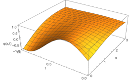
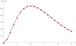
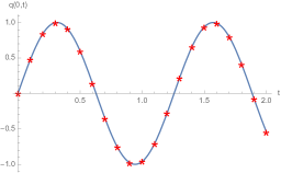
Figure 6.1. Evaluation of the novel solution formula (3.9) for the $q$-component of IBVP (1.2) with initial data $q_{0}(x)=x^{2}e^{-x}$ and boundary data $g_{0}(t)=\sin(5t)$. Left panel: The solution $q$ as a function of $(x,t)\in(0,3)\times(0,1)$. Center panel: The solution $q$ at $t=0$ as a function of $x\in(0,5)$. Right panel: The solution $q$ at $x=0$ as a function of $t\in(0,2)$. The red stars in the center and right panels represent the precise values of the data $q_{0}(x)$ and $g_{0}(t)$, respectively, showing perfect agreement of formula (3.9) with the prescribed data. Of particular importance for the third plot is the uniform convergence of formula (3.9) at the boundary $x=0$.

Furthermore, formula (3.9) was rederived in Section 4 from a different starting point, namely by reducing system (1.2a) to a single equation. This reduction is not possible for general dispersive systems, which is the main reason why the systems approach of Section 2 is preferable; however, the second approach demonstrates the versatility of the unified transform method and offers a different perspective concerning the types of admissible boundary data. Moreover, to the best of our knowledge, the analysis of Section 4 signifies the first time that the unified transform method has been applied to an equation whose dispersion relation is a quotient involving a complex square root (and hence branching), due to the presence of the mixed derivative $\left(1-\partial_{x}^{2}\right)\partial_{t}^{2}$.

We emphasize that the present article is not the first one devoted to the linearized classical Boussinesq IBVP (1.2) via the unified transform method. Indeed, Fokas and Pelloni had previously considered the same problem in [FP1]. Importantly, however, their approach was entirely different, as they utilized the nonlinear component of the unified transform method, which relies on formulating IBVP (1.2) as a Lax pair and then integrating it by using ideas inspired from the inverse scattering transform, namely by associating it with a Riemann-Hilbert problem which is then solved via Plemelj’s formulae. The complexity of those techniques naturally limits the accessibility of the derivation of [FP1] to a very specialized audience. In contrast, the present work employs the linear component of the unified transform method, which only requires knowledge of Fourier transform and Cauchy’s theorem from complex analysis and hence is accessible to a broad audience within the applied sciences.

Another significant difference between the present work and [FP1] is the fact that, due to the nature of the Riemann-Hilbert problem, the resulting solution formula in [FP1] involves certain principal value integrals. The presence of these integrals seems unsuitable for the purpose of effective numerical implementations. Furthermore, it will most likely pose an issue when attempting to use that formula for establishing well-posedness of the original, nonlinear classical Boussinesq system (1.1) via the contraction mapping approach (see relevant discussion in the introduction). On the other hand, the novel solution formula derived in this article does not involve any singularities and hence is expected to be effective for showing well-posedness of the classical Boussinesq system (1.1) on the half-line via the contraction mapping approach, along the lines of [FHM1, FHM2, HM2, HM3].

Acknowledgements. The first author would like to thank the Department of Mathematics of the University of Kansas for partially supporting their research through an undergraduate research award. All three authors are grateful to Andre Kurait for inspiring discussions during the 2018-19 academic year that paved the way to the present work. Finally, the authors are thankful to the reviewers of the manuscript for useful remarks and suggestions.

References

• [AbF] M. Ablowitz and A. Fokas, Complex variables: introduction and applications, Cambridge University Press, 2003 (2nd edition).
• [Ad] K. Adamy, Existence of solutions for a Boussinesq system on the half line and on a finite interval. Discrete Contin. Dyn. Syst. 29 (2011), 25-49.
• [AL] B. Alvarez-Samaniego and D. Lannes, Large time existence for 3D water-waves and asymptotics. Invent. Math. 171 (2008), 485-541.
• [Am] C. Amick, Regularity and uniqueness of solutions to the Boussinesq system of equations. J. Differential Equations 54 (1984), 231-247.
• [AnF] Y. Antipov and A. Fokas, The modified Helmholtz equation in a semi-strip. Math. Proc. Cambridge Philos. Soc. 138 (2005), 339-365.
• [AD] D. Antonopoulos and V. Dougalis, Numerical solution of the “classical” Boussinesq system. Math. Comput. Simul. 82 (2012), 984-1007.
• [BCS1] J. Bona, M. Chen and J.-C. Saut, Boussinesq equations and other systems for small-amplitude long waves in nonlinear dispersive media I: Derivation and linear theory. J. Nonlinear Sci. 12 (2002), 283-318.
• [BCS2] J. Bona, M. Chen and J.-C. Saut, Boussinesq equations and other systems for small-amplitude long waves in nonlinear dispersive media II: The nonlinear theory. Nonlinearity 17 (2004), 925-952.
• [B1] J. Boussinesq, Théorie des ondes et des remous qui se propagent le long d’un canal rectangulaire horizontal, en communiquant au liquide contenu dans ce canal des vitesses sensiblement pareilles de la surface au fond. J. Math. Pures Appl. 17 (1872), 55-108.
• [B2] J. Boussinesq, Essai sur la théorie des eaux courantes. Mémoires présentés par divers savants à l’Académie des Sciences 23 (1877), 1-680.
• [CFF] M. Colbrook, N. Flyer and B. Fornberg, On the Fokas method for the solution of elliptic problems in both convex and non-convex polygonal domains. J. Comput. Phys. 374 (2018), 996-1016.
• [DGSV] B. Deconinck, Q. Guo, E. Shlizerman and V. Vasan, Fokas’s unified transform method for linear systems. Quart. Appl. Math. 76 (2018), 463-488.
• [DSS] B. Deconinck, N. Sheils and D. Smith, The linear KdV equation with an interface. Comm. Math. Phys. 347 (2016), 489-509.
• [DTV] B. Deconinck, T. Trogdon and V. Vasan, The method of Fokas for solving linear partial differential equations. SIAM Rev. 56 (2014), 159-186.
• [F1] A. Fokas, A unified transform method for solving linear and certain nonlinear PDEs. Proc. R. Soc. A 453 (1997), 1411-1443.
• [F2] A. Fokas, A unified approach to boundary value problems, CBMS-NSF Regional Conference Series in Applied Mathematics 78, SIAM, Philadelphia, PA, 2008.
• [FFSS] A. Fokas, N. Flyer, S. Smitheman and E. Spence, A semi-analytical numerical method for solving evolution and elliptic partial differential equations. J. Comput. Appl. Math. 227 (2009), 59-74.
• [FHM1] A. Fokas, A. Himonas and D. Mantzavinos, The Korteweg-de Vries equation on the half-line. Nonlinearity 29 (2016), 489-527.
• [FHM2] A. Fokas, A. Himonas and D. Mantzavinos, The nonlinear Schrödinger equation on the half-line. Trans. Amer. Math. Soc. 369 (2017), 681-709.
• [FI] A. Fokas and A. Its, The nonlinear Schrödinger equation on the interval. J. Phys. A: Math. Gen. 37 (2004), 6091-6114.
• [FK] A. Fokas and A. Kapaev, On a transform method for the Laplace equation in a polygon. IMA J. Appl. Math. 68 (2003), 355-408.
• [FL] A. Fokas and J. Lenells, The unified method: I. Nonlinearizable problems on the half-line. J. Phys. A 45 (2012), 195201.
• [FF] N. Flyer and A. Fokas, A hybrid analytical numerical method for solving evolution partial differential equations. I: the half-line. Proc. R. Soc. 464 (2008), 1823-1849.
• [FP1] A. Fokas and B. Pelloni, Boundary value problems for Boussinesq type systems. Math. Phys. Anal. Geom. 8 (2005), 59-96.
• [FP2] A. Fokas and B. Pelloni, Unified transform for boundary value problems: applications and advances, SIAM, Philadelphia, PA, 2015.
• [FS] A. Fokas and E. Spence, Synthesis, as opposed to separation, of variables. SIAM Rev. 54 (2012), 291-324.
• [HM1] A. Himonas and D. Mantzavinos, On the initial-boundary value problem for the linearized Boussinesq equation. Stud. Appl. Math. 134 (2015), 62-100.
• [HM2] A. Himonas and D. Mantzavinos, The “good” Boussinesq equation on the half-line. J. Differential Equations 258 (2015), 3107-3160.
• [HM3] A. Himonas and D. Mantzavinos, Well-posedness of the nonlinear Schrödinger equation on the half-plane. Nonlinearity 33 (2020), 5567-5609.
• [KO] K. Kalimeris and T. Ozsari, An elementary proof of the lack of null controllability for the heat equation on the half line. Appl. Math. Lett. 104 (2020), 106241.
• [L] D. Lannes, The water waves problem: mathematical analysis and asymptotics, Amer. Math. Soc., 2013.
• [LW] D. Lannes and L. Weynans, Generating boundary conditions for a Boussinesq system. Nonlinearity 33 (2012), 6868-6889.
• [MID] D. Mitsotakis, B. Ilan and D. Dutykh, On the Galerkin/finite-element method for the Serre equations. J. Sci. Comput. 61 (2014), 166-195.
• [MTZ] L. Molinet, R. Talhouk and I. Zaiter, The classical Boussinesq system revisited. arXiv :2001.11870v1 (2020).
• [P] D. Peregrine, Long waves on a beach. J. Fluid Mech. 27 (1967), 815-827.
• [S] M. Schonbeck, Existence of solutions for the Boussinesq system of equations. J. Differential Equations 42 (1981), 325-352.
• [SSF] S. Smitheman, E. Spence and A. Fokas, A spectral collocation method for the Laplace and modified Helmholtz equations in a convex polygon. IMA J. Numer. Anal. 30 (2010), 1184-1205.
• [VD] V. Vasan and B. Deconinck, Well-posedness of boundary-value problems for the linear Benjamin-Bona-Mahony equation. Discrete Contin. Dyn. Syst. 33 (2013), 3171-3188.