Exploring the Linear Subspace
Hypothesis in Gender Bias Mitigation

Abstract

Bolukbasi et al. (2016) presents one of the first gender bias mitigation techniques for word embeddings. Their method takes pre-trained word embeddings as input and attempts to isolate a linear subspace that captures most of the gender bias in the embeddings. As judged by an analogical evaluation task, their method virtually eliminates gender bias in the embeddings. However, an implicit and untested assumption of their method is that the bias subspace is actually linear. In this work, we generalize their method to a kernelized, non-linear version. We take inspiration from kernel principal component analysis and derive a non-linear bias isolation technique. We discuss and overcome some of the practical drawbacks of our method for non-linear gender bias mitigation in word embeddings and analyze empirically whether the bias subspace is actually linear. Our analysis shows that gender bias is in fact well captured by a linear subspace, justifying the assumption of Bolukbasi et al. (2016).

1 Introduction

Pre-trained word representations are a necessity for strong performance on modern NLP tasks. These embeddings now serve as input to neural methods Goldberg (2017), which recently have become the standard models in the field. However, because these representations are constructed from large, human-created corpora, they naturally contain societal biases encoded in that data; gender bias is among the most well studied of these biases Caliskan et al. (2017). Both a-contextual word embeddings Mikolov et al. (2013); Pennington et al. (2014) and contextual word embeddings Peters et al. (2018); Devlin et al. (2019) have been shown to encode gender bias Bolukbasi et al. (2016); Caliskan et al. (2017); Zhao et al. (2019); May et al. (2019); Karve et al. (2019). More importantly, the bias in those embeddings has been shown to influence models for downstream tasks where they are used as input, e.g. coreference resolution (Rudinger et al., 2018; Zhao et al., 2018).

Bolukbasi et al. (2016) present one of the first methods for detecting and mitigating gender bias in word embeddings. They provide a novel linear-algebraic approach that post-processes word embeddings in order to partially remove gender bias. Under their evaluation, they find they can nearly perfectly remove bias in an analogical reasoning task. However, subsequent work Gonen and Goldberg (2019); Hall Maudslay et al. (2019) has indicated that gender bias still lingers in the embeddings, despite Bolukbasi et al. (2016)'s strong experimental results. In the development of their method, Bolukbasi et al. (2016) make a critical and unstated assumption: Gender bias forms a linear subspace of word embedding space. In mathematics, linearity is a strong assumption and there is no reason a-priori why one should expect complex and nuanced societal phenomena, such as gender bias, should be represented by a linear subspace.

In this work, we present the first non-linear gender bias mitigation technique for a-contextual word embeddings. In doing so, we directly test the linearity assumption made by Bolukbasi et al. (2016). Our method is based on the insight that Bolukbasi et al. (2016)'s method bears a close resemblance to principal component analysis (PCA). Just as one can kernelize PCA Schölkopf et al. (1997), we show that one can kernelize the method of Bolukbasi et al. (2016). Due to the kernelization, the bias is removed in the feature space, rather in the word embedding space. Thus, we also explore pre-image techniques Mika et al. (1999) to project the bias-mitigated vectors back into $\mathbb{R}^{d}$.

As previously noted, there are now multiple bias removal methodologies (Zhao et al., 2018, 2019; May et al., 2019) that have succeed the method by Bolukbasi et al. (2016). Furthermore Gonen and Goldberg (2019) point out multiple flaws in Bolukbasi et al. (2016)'s bias mitigation technique and the aforementioned methods. Nonetheless we believe that this method has received sufficient attention from the community such that research into its properties is both interesting and useful.

We test our non-linear gender bias technique in several experiments. First, we consider the Word Embedding Association Test (WEAT; Caliskan et al., 2017); we notice that across five non-linear kernels and convex combinations thereof, there is seemingly no significant difference between the non-linear bias mitigation technique and the linear one. Secondly, we consider the professions task Bolukbasi et al. (2016); Gonen and Goldberg (2019) that measures how word embeddings representing different professions are potentially gender-stereotyped. Again, as with the WEAT evaluation, we find that our non-linear bias mitigation technique performs on par with the linear method. We also consider whether the non-linear gender mitigation technique removes indirect bias from the vectors Gonen and Goldberg (2019); yet again, we find the non-linear method performs on par with the linear methods. As a final evaluation, we evaluate whether non-linear bias mitigation hurts semantic performance. On Simlex-999 Hill et al. (2015), we show that similarity estimates between the vectors remain on par with the linear methods. We conclude that much of the gender bias in word embeddings is indeed captured by a linear subspace, answering this paper's titular question.

2 Bias as a Linear Subspace

The first step of Bolukbasi et al. (2016)'s technique is the discovery of a subspace $B\subset\mathbb{R}^{d}$ that captures most of the gender bias. Specifically, they stipulate that this space is linear. Given word embeddings that live in $\mathbb{R}^{d}$, they provide a spectral method for isolating the bias subspace. In this section, we review their approach and show how it is equivalent to principal component analysis (PCA) on a specific design (input) matrix. Then, we introduce and discuss the implicit assumption made by their work; we term this assumption the linear subspace hypothesis and test it in § 4.

Hypothesis 1.

Gender bias in word embeddings may be represented as a linear subspace.

2.1 Construction of a Bias Subspace

We will assume the existence of a fixed and finite vocabulary $V$, each element of which is a word $\mathbf{w}_{i}$. The hard-debiasing approach takes a set of $N$ sets $\mathcal{D}=\{D_{n}\}_{n=1}^{N}$ as input. Each set $D_{n}$ contains words that are considered roughly semantically equivalent modulo their gender; Bolukbasi et al. (2016) call the $D_{n}$ defining sets. For example, $\{\textit{man},\textit{woman}\}$ and $\{\textit{he},\textit{she}\}$ form two such defining sets. We identify each word with a unique integer $i$ for the sake of our indexing notation; indeed, we exclusively reserve the index $i$ for words. We additionally introduce the function $f:[|V|]\rightarrow[N]$ that maps an individual word to its defining set. In general, the defining sets are not limited to a cardinality of two, but in practice Bolukbasi et al. (2016) exclusively employ defining sets with a cardinality of two in their experiments. Using the sets $D_{n}$, Bolukbasi et al. (2016) define the matrix ${\bm{C}}$

$${\bm{C}}:=\sum_{n=1}^{N}\frac{1}{|D_{n}|}\sum_{i\in D_{n}}\left(\mathbf{w}_{i}-{\bm{\mu}}_{D_{n}}\right)\left(\mathbf{w}_{i}-{\bm{\mu}}_{D_{n}}\right)^{\top}$$

where we write $\mathbf{w}_{i}$ for the $i^{\text{th}}$ word's embedding and the empirical mean vector ${\bm{\mu}}_{D_{n}}$ is defined as

$${\bm{\mu}}_{D_{n}}:=\frac{1}{|D_{n}|}\sum_{i\in D_{n}}\mathbf{w}_{i}$$

Bolukbasi et al. (2016) then extract a bias subspace $B$ using the singular value decomposition (SVD). Specifically, they define the bias subspace to be the space spanned by the first $k$ columns of ${\bm{V}}$ where

$${\bm{V}}{\bm{S}}{\bm{V}}^{\top}=\operatorname{SVD}({\bm{C}})$$ (1)

Since ${\bm{C}}$ is symmetric and positive semi-definite, the SVD is equivalent to an eigendecomposition as our notation in Equation 1 shows. We assume the columns of ${\bm{V}}$, the eigenvectors of ${\bm{C}}$, are ordered by the magnitude of their corresponding eigenvalues.

2.2 Bias Subspace Construction as PCA

As briefly noted by Bolukbasi et al. (2016), this can thus be cast as performing principal component analysis (PCA) on a recentered input matrix. We prove this assertion more formally. We first prove that the matrix ${\bm{C}}$ may be written as an empirical covariance matrix.

Proposition 1.

Suppose $|D_{n}|=2$ for all $n$. Then we have

$${\bm{C}}=\frac{1}{2}\sum_{i=1}^{2N}{\bm{W}}_{i,\cdot}^{\top}\,{\bm{W}}_{i,\cdot}$$ (2)

where we define the design matrix ${\bm{W}}$ as:

$${\bm{W}}_{i,\cdot}=\left(\mathbf{w}_{i}-{\bm{\mu}}_{D_{f(i)}}\right)^{\top}$$ (3)

Proof.

$${\bm{C}} =\sum_{n=1}^{N}\frac{1}{|D_{n}|}\sum_{i\in D_{n}}\left(\mathbf{w}_{i}-{\bm{\mu}}_{D_{n}}\right)\left(\mathbf{w}_{i}-{\bm{\mu}}_{D_{n}}\right)^{\top}$$

$$=\frac{1}{2}\sum_{n=1}^{N}\sum_{i\in D_{n}}\left(\mathbf{w}_{i}-{\bm{\mu}}_{D_{n}}\right)\left(\mathbf{w}_{i}-{\bm{\mu}}_{D_{n}}\right)^{\top}$$

$$=\frac{1}{2}\sum_{i=1}^{2N}\left(\mathbf{w}_{i}-{\bm{\mu}}_{D_{f(i)}}\right)\left(\mathbf{w}_{i}-{\bm{\mu}}_{D_{f(i)}}\right)^{\top}$$

$$=\frac{1}{2}\sum_{i=1}^{2N}{\bm{W}}_{i,\cdot}^{\top}\,{\bm{W}}_{i,\cdot}$$

where ${\bm{W}}_{i,\cdot}\in\mathbb{R}^{2N\times d}$ is defined as above. ∎

Next, we show that the matrix is centered, which is a requirement for PCA.

Proposition 2.

The matrix ${\bm{W}}$ is row-wise centered.

Proof.

$$\frac{1}{2}\sum_{i=1}^{2N}{\bm{W}}_{i,\cdot}^{\top} =\frac{1}{2}\sum_{i=1}^{2N}\left(\mathbf{w}_{i}-{\bm{\mu}}_{D_{f(i)}}\right)$$

$$=\frac{1}{2}\sum_{n=1}^{N}\sum_{i\in\mathcal{D}_{n}}\left(\mathbf{w}_{i}-{\bm{\mu}}_{D_{n}}\right)$$

$$=\frac{1}{2}\sum_{n=1}^{N}\left(-2{\bm{\mu}}_{D_{n}}+\sum_{i\in\mathcal{D}_{n}}\mathbf{w}_{i}\right)$$

$$=\frac{1}{2}\sum_{n=1}^{N}\left(2{\bm{\mu}}_{D_{n}}-2{\bm{\mu}}_{D_{n}}\right)=0$$

∎

Remark 3.

The method of Bolukbasi et al. (2016) may be considered principal component analysis performed on the matrix $2{\bm{C}}$.

Proof.

As the algebra in proposition 1 and proposition 2 show we may formulate the problem as an SVD on a mean-centered covariance matrix. One view of PCA is performing matrix factorization on such a matrix. ∎

3 Bolukbasi et al. (2016)

In this section, we review the bias mitigation technique introduced by Bolukbasi et al. (2016). When possible, we take care to reformulate their method in terms of matrix notation. They introduce a two-step process that neutralizes and equalizes the vectors to mitigate gender bias in the embeddings. The underlying assumption of their method is that there exists a linear subspace $B\subset\mathbb{R}^{d}$ that captures most of the gender bias.

3.1 Neutralize

After finding the linear bias subspace $B$, the gist behind Bolukbasi et al. (2016)'s approach is based on elementary linear algebra. We may decompose any word vector $\mathbf{w}$ as the sum of its orthogonal projection onto the bias subspace (range of the projection) and its orthogonal projection onto the complement of the bias subspace (null space of the projection), i.e.

$$\mathbf{w}=\mathbf{w}_{B}+\mathbf{w}_{\perp B}$$ (4)

We may then re-embed every vector as

$$\mathbf{w}_{\mathrm{ntr}}:=\mathbf{w}-\mathbf{w}_{B}=\mathbf{w}_{\perp B}$$ (5)

We may re-write this in terms of matrix notation in the following manner. Let $\{\mathbf{v}_{k}\}_{k=1}^{K}$ be an orthogonal basis for the linear bias subspace $B$. This may be found by taking the eigenvectors ${\bm{C}}$ that correspond to the top-$K$ eigenvalues with largest magnitude. Then, we define the projection matrix onto the bias subspace as ${\bm{P}}_{K}=\sum_{k=1}^{K}\mathbf{v}_{k}\mathbf{v}_{k}^{\top}$ it follows that the matrix $({\bm{I}}-{\bm{P}}_{K})$ is a projection matrix on the complement of $B$. We can then write the neutralize step using matrices

$$\mathbf{w}_{\mathrm{ntr}}:=({\bm{I}}-{\bm{P}}_{K})\,\mathbf{w}$$ (6)

The matrix formulation of the neutralize step offers a cleaner presentation of what the neutralize step does: it projects the vectors onto the orthogonal complement of the bias subspace.

3.2 Equalize

Bolukbasi et al. (2016) decompose words into two classes. The neutral words which undergo neutralization as explained above, and the gendered words, some of which receive the equalizing treatment. Given a set of equality sets $\mathcal{E}=\{E_{1},\ldots,E_{L}\}$ which we can see as a greater extension of the defining sets $\mathcal{D}$, i.e. $E_{i}=\{\textit{guy},\textit{gal}\}$, Bolukbasi et al. (2016) then proceed to decompose each of the words $\mathbf{w}\in\mathcal{E}$ into their gendered and neutral counterparts, setting their neutral component to a constant (the mean of the equality set) and the gendered component to its mean-centered projection into the gendered subspace:

$$\mathbf{w}_{\mathrm{eq}}:={\bm{\nu}}+Z\,(\mathbf{w}_{B}-{\bm{\mu}}_{B})$$ (7)

where we define the following quantities:

$$Z:=\frac{\sqrt{1-||{\bm{\nu}}||_{2}^{2}}}{||\mathbf{w}_{B}-{\bm{\mu}}_{B}||_{2}}\,$$

$${\bm{\mu}}:=\frac{1}{|E_{i}|}\sum_{\mathbf{w}\in E_{i}}\mathbf{w}$$

$${\bm{\nu}}:=({\bm{I}}-{\bm{P}}_{K})\,{\bm{\mu}}$$

the ``normalizer'' $Z$ ensures the vector is of unit length. This fact is left unexplained in the original work, but Hall Maudslay et al. (2019) provide a proof in their appendix.

4 Bias as a Non-Linear Subspace

We generalize the framework presented in Bolukbasi et al. (2016) and cast it to a non-linear setting by exploiting its relationship to PCA. Thus, the natural extension of Bolukbasi et al. (2016) is to kernelize it analogously to Schölkopf et al. (1997), which is the kernelized generalization of PCA. Our approach preserves all the desirable formal properties presented in the linear method of Bolukbasi et al. (2016).

4.1 Adapting the Design Matrix

The idea behind our non-linear bias mitigation technique is based on kernel PCA Schölkopf et al. (1998). In short, the idea is to map the original word embeddings $\mathbf{w}_{i}\in\mathbb{R}^{d}$ to a higher-dimensional space ${\mathcal{H}}$ via a function ${\bm{\Phi}}:\mathbb{R}^{d}\rightarrow{\mathcal{H}}$. We will consider cases where ${\mathcal{H}}$ is a reproducing kernel Hilbert space (RKHS) with reproducing kernel $\kappa(\mathbf{w}_{i},\mathbf{w}_{j})=\langle{\bm{\Phi}}(\mathbf{w}_{i}),{\bm{\Phi}}(\mathbf{w}_{j})\rangle$ where the notation $\langle\cdot,\cdot\rangle$ refers to an inner product in the RKHS. Traditionally, one calls ${\mathcal{H}}$ the feature space and will use this terminology throughout this work. Exploiting the reproducing kernel property, we may carry out Bolukbasi et al. (2016)'s bias isolation technique and construct a non-linear analogue.

We start the development of bias mitigation technique in feature space with a modification of the design matrix presented in Eq. 3. In the RKHS setting the non-linear analogue is

$${\bm{W}}^{{\bm{\Phi}}}_{i,\cdot}:={\bm{\Phi}}(\mathbf{w}_{i})-{\bm{M}}^{{\bm{\Phi}}}_{D_{f}(i)},\quad\forall\,\mathbf{w}_{i}\in V$$ (8)

where we define

$${\bm{M}}^{{\bm{\Phi}}}_{D_{n}}:=\frac{1}{|D_{n}|}\sum_{i\in D_{n}}{\bm{\Phi}}(\mathbf{w}_{i})$$ (9)

As one can see, this is a relatively straightforward mapping from the set of linear operations to non-linear ones.

4.2 Kernel PCA

Using our modified design matrix, we can cast our non-linear bias mitigation technique as a form of kernel PCA. Specifically, we form the following matrix

$${\bm{C}}^{{\bm{\Phi}}} =\frac{1}{2}\sum_{i=1}^{2N}({\bm{W}}^{{\bm{\Phi}}}_{i,\cdot})^{\top}{\bm{W}}^{{\bm{\Phi}}}_{i,\cdot}$$

Our goal is to find the eigenvalues $\lambda_{k}$ and their corresponding eigenfunctions ${\bm{V}}_{k}^{{\bm{\Phi}}}\in{\mathcal{H}}$ by solving the eigenvalue problem

$${\bm{C}}^{{\bm{\Phi}}}\,{\bm{V}}^{{\bm{\Phi}}}_{k} =\lambda_{k}{\bm{V}}^{{\bm{\Phi}}}_{k}$$ (10)

Computing these directly from Equation 10 is impossible since ${\mathcal{H}}$'s dimension may be prohibitively large or even infinite. However, Schölkopf et al. note that ${\bm{V}}_{k}^{{\bm{\Phi}}}$ is spanned by $\{{\bm{\Phi}}(\mathbf{w}_{i})\}_{i=1}^{2N}$. This allows us to rewrite Eq. 10 as

$${\bm{V}}^{{\bm{\Phi}}}_{k}=\sum_{i=1}^{2N}\alpha^{k}_{i}\,{\bm{\Phi}}(\mathbf{w}_{i})$$ (11)

where there exist coefficients $\alpha^{k}_{i}\in\mathbb{R}$. Now, by substituting Eq. 11 and Eq. 10 into the respective terms in $\lambda\langle{\bm{\Phi}}(\mathbf{w}_{i}),{\bm{V}}_{k}^{{\bm{\Phi}}}\rangle=\langle{\bm{\Phi}}(\mathbf{w}_{i}),{\bm{C}}\,{\bm{V}}_{k}^{{\bm{\Phi}}}\rangle$, Schölkopf et al. (1997) derive a computationally feasible eigendecomposition problem. Specifically, they consider

$$2N\lambda_{k}\,{\bm{\alpha}}^{k}={\bm{K}}{\bm{\alpha}}^{k}$$ (12)

where ${\bm{K}}_{ij}=\langle{\bm{\Phi}}(\mathbf{w}_{i}),{\bm{\Phi}}(\mathbf{w}_{j})\rangle$. Once all the ${\bm{\alpha}}^{k}$ vectors have been estimated the inner product between an eigenfunction ${\bm{V}}_{k}^{{\bm{\Phi}}}$ and a point $\mathbf{w}$ can be computed as

$$\beta_{k}(\mathbf{w}) =\langle{\bm{V}}^{{\bm{\Phi}}}_{k},{\bm{\Phi}}(\mathbf{w}_{i})\rangle$$

$$=\sum_{i=1}^{2N}\alpha_{i}^{k}\,\kappa(\mathbf{w}_{i},\mathbf{w})$$ (13)

A projection into the basis $\{{\bm{V}}^{{\bm{\Phi}}}_{k}\}_{k=1}^{K}$ can then be carried out by applying the projection operator $\operatorname{P}_{K}:{\mathcal{H}}\rightarrow{\mathcal{H}}$ as follows:

$$\operatorname{P}_{K}{\bm{\Phi}}(\mathbf{w})=\sum_{k=1}^{K}\beta_{k}(\mathbf{w})\,{\bm{V}}^{{\bm{\Phi}}}_{k}$$ (14)

where $K$ is the number of principal components. Projection operator $\operatorname{P}_{K}$ is analogous to the linear projection ${\bm{P}}_{K}$ introduced in § 3.1.

4.3 Centering Kernel Matrix

We can perform the required mean-centering operations on the design matrix by centering the kernel matrix in a similar fashion to Schölkopf et al. (1998). For the case of equality sets of size 2, which is what Bolukbasi et al. use in practice, we realize that the centered design matrix reduces to pairwise differences:

$${\bm{W}}^{{\bm{\Phi}}}_{i,\cdot} =\frac{1}{2}({\bm{\Phi}}(\mathbf{w}_{i})-{\bm{\Phi}}(\mathbf{w}_{j})),$$ (15)

$$\quad\quad\quad\mathbf{w}_{i},\mathbf{w}_{j}\in D_{n}\wedge\mathbf{w}_{j}\neq\mathbf{w}_{i}$$

which leads to a very simple re-centering in terms of the Gram matrices:

$$\tilde{{\bm{K}}}={\bm{K}}^{(11)}-{\bm{K}}^{(12)}-({\bm{K}}^{(12)})^{\top}+{\bm{K}}^{(22)}$$

where

$${\bm{K}}^{(xy)}_{ij} =\frac{1}{2}\kappa\left({\bm{W}}^{(x)}_{i,\cdot},{\bm{W}}^{(y)}_{j,\cdot}\right),$$

$${\bm{W}}^{(z)}_{i.\cdot} =\begin{cases}\mathbf{w}_{\pi_{1+i\text{\,mod\,}2}(\hat{f}({\lceil\frac{i}{2}\rceil}))}&z=1\\ \mathbf{w}_{\pi_{2-i\text{\,mod\,}2}(\hat{f}({\lceil\frac{i}{2}\rceil}))}&z=2\end{cases}$$ (16)

where $\hat{f}:[N]\rightarrow[|V|]\times[|V|]$ maps a defining set index to a tuple containing the word indices in the corresponding defining set and $\pi_{1},\pi_{2}:[|V|]\times[|V|]\rightarrow[|V|]$ are projection operators which return the first or second elements of a tuple respectively. In simpler terms, Eq. 16 is creating two matrices: matrix ${\bm{W}}^{(1)}$ which is constructed by looping over the definition sets and placing pairs within the same definition set as adjacent rows, then ${\bm{W}}^{(2)}$ is constructed in the same way but the order of the adjacent pairs is swapped relative to ${\bm{W}}^{(1)}$. Once we have this pairwise centered Gram matrix $\tilde{{\bm{K}}}$ we can apply the eigendecomposition procedure described in Equation 12 directly on $\tilde{{\bm{K}}}$. We note that carrying out this procedure using a linear kernel recovers the linear bias subspace from Bolukbasi et al. (2016).

4.4 Inner Product Correction (Neutralize)

We now focus on neutralizing and equalizing the inner products in the RKHS rather than correcting the word embeddings directly. Just as in the linear case, we can decompose the representation of a word in the RKHS into biased and neutral components

$${\bm{\Phi}}(\mathbf{w})=\operatorname{P}_{K}^{\perp}{\bm{\Phi}}(\mathbf{w})+\operatorname{P}_{K}{\bm{\Phi}}(\mathbf{w}),$$ (17)

which provides a nonlinear equivalent for Eq. 6

$${{\bm{\Phi}}_{\mathrm{ntr}}}(\mathbf{w}) =\operatorname{P}_{K}^{\perp}{\bm{\Phi}}(\mathbf{w})$$ (18)

$$={\bm{\Phi}}(\mathbf{w})-\operatorname{P}_{K}{\bm{\Phi}}(\mathbf{w})$$

Proposition 4.

The corrected inner product in the feature space for two neutralized words $\mathbf{z},\mathbf{w}$ is given by

$$\langle{{\bm{\Phi}}_{\mathrm{ntr}}} (\mathbf{z}),{{\bm{\Phi}}_{\mathrm{ntr}}}(\mathbf{w})\rangle$$ (19)

$$=\kappa(\mathbf{z},\mathbf{w})-\sum_{k=1}^{K}\beta_{k}(\mathbf{z})\,\beta_{k}(\mathbf{w})$$

Proof.

$$\Big{<} {{\bm{\Phi}}_{\mathrm{ntr}}}(\mathbf{z}),{{\bm{\Phi}}_{\mathrm{ntr}}}(\mathbf{w})\Big{>}=$$

$$\Big{<}{\bm{\Phi}}(\mathbf{z})-\operatorname{P}_{K}{\bm{\Phi}}(\mathbf{z}),\>{\bm{\Phi}}(\mathbf{w})-\operatorname{P}_{K}{\bm{\Phi}}(\mathbf{w})\Big{>}$$

Applying Eq. 13 and Eq. 14

$$=\kappa(\mathbf{z},\mathbf{w})-\sum_{k=1}^{K}\beta_{k}(\mathbf{w})\sum_{i=1}^{2N}\alpha_{i}^{k}\kappa(\mathbf{z},\mathbf{w}_{i})$$

$$-\sum_{k=1}^{K}\beta_{k}(\mathbf{z})\sum_{i=1}^{2N}\alpha_{i}^{k}\kappa(\mathbf{w},\mathbf{w}_{i})+\sum_{k=1}^{K}\beta_{k}(\mathbf{w})\beta_{k}(\mathbf{z})$$

$$=\kappa(\mathbf{z},\mathbf{w})-\sum_{k=1}^{K}\beta_{k}(\mathbf{w})\sum_{i=1}^{2N}\alpha_{n}^{k}\kappa(\mathbf{z},\mathbf{w}_{i})$$

$$=\kappa(\mathbf{z},\mathbf{w})-\sum_{k=1}^{K}\beta_{k}(\mathbf{w})\beta_{k}(\mathbf{z}),$$ (20)

where

$$\beta_{k}(\mathbf{w})=\bm{V}_{k}^{{\bm{\Phi}}\top}{\bm{\Phi}}(\mathbf{w})=\sum_{i=1}^{2N}\alpha_{i}^{k}\,\kappa(\mathbf{w},\mathbf{w}_{i})$$

as derived by Schölkopf et al. (1998). ∎

An advantage of this approach is that it will not rely on errors due to the approximation of the pre-image. However, it will not give us back a set of debiased embeddings. Instead, it returns a debiased metric, thus limiting the classifiers and regressors we could use. Equation Eq. 19 provides us with an $\mathcal{O}(KNd)$ approach to compute the inner product between two feature-space neutralized words.

4.5 Inner Product Correction (Equalize)

To equalize, we may naturally convert Eq. 7 to its feature-space equivalent. We define an equalizing function

$${\bm{\theta}}_{\mathrm{eq}}(\mathbf{w}_{i}) :={\bm{\nu}}^{{\bm{\Phi}}}+Z^{{\bm{\Phi}}}\,\operatorname{P}_{K}\left({\bm{\Phi}}(\mathbf{w}_{i})-{\bm{M}}^{{\bm{\Phi}}}_{E_{g(i)}}\right)$$

where we define

$${\bm{\nu}}^{{\bm{\Phi}}} :=\operatorname{P}_{K}^{\perp}{\bm{M}}^{{\bm{\Phi}}}_{E_{g(i)}}$$

$$Z^{{\bm{\Phi}}} :=\frac{\sqrt{1-||\nu_{{\bm{\Phi}}}||^{2}}}{||\operatorname{P}_{K}({\bm{\Phi}}(\mathbf{w})-{\bm{M}}^{{\bm{\Phi}}}_{E_{g(i)}})||}$$

where $g:[|V|]\rightarrow[L]$ maps an individual word index to its corresponding equality set index. Given vector dot products in the linear case follow the same geometric properties as inner products in the RKHS we can show that ${\bm{\theta}}_{\mathrm{eq}}(\mathbf{w})$ is unit norm follows directly from the proof for Proposition 1 in Hall Maudslay et al. (2019) which can be found in Appendix A of Hall Maudslay et al. (2019).

Proposition 5.

For any two vectors in the observed space $\mathbf{w},\mathbf{z}$ and their corresponding representations in feature space ${\bm{\Phi}}(\mathbf{w}),{\bm{\Phi}}(\mathbf{z})$ the inner product $\langle{\bm{\Phi}}(\mathbf{w})-\operatorname{P}_{K}{\bm{\Phi}}(\mathbf{w}),\operatorname{P}_{K}{\bm{\Phi}}(\mathbf{z})\rangle$ is $0$.

Proof.

$$\langle{\bm{\Phi}} (\mathbf{w})-\operatorname{P}_{K}{\bm{\Phi}}(\mathbf{w}),\operatorname{P}_{K}{\bm{\Phi}}({\bm{e}})\rangle$$

$$=\langle{\bm{\Phi}}(\mathbf{w}),\operatorname{P}_{K}{\bm{\Phi}}(\mathbf{z})\rangle-\langle\operatorname{P}_{K}{\bm{\Phi}}(\mathbf{w}),\operatorname{P}_{K}{\bm{\Phi}}(\mathbf{z})\rangle$$

$$=\sum_{k=1}^{K}\beta_{k}(\mathbf{w})\beta_{k}(\mathbf{z})-\sum_{k=1}^{K}\beta_{k}(\mathbf{w})\beta_{k}(\mathbf{z})=0$$

∎

Proposition 6.

For a given neutral word $\mathbf{w}$ and a word in an equality set ${\bm{e}}\in\mathcal{E}$ the inner product $\left<{{\bm{\Phi}}_{\mathrm{ntr}}}(\mathbf{w}),{\bm{\theta}}_{\mathrm{eq}}({\bm{e}})\right>$ is invariant across members in the equality set $\mathcal{E}$.

Proof.

$$\langle {{\bm{\Phi}}_{\mathrm{ntr}}}(\mathbf{w}),{\bm{\theta}}_{\mathrm{eq}}({\bm{e}})\rangle\overset{\textit{(}i)}{=}\langle{{\bm{\Phi}}_{\mathrm{ntr}}}(\mathbf{w}),{\bm{\nu}}^{{\bm{\Phi}}}\rangle$$

$$=\frac{1}{|E|}\sum_{i\in E}\langle{{\bm{\Phi}}_{\mathrm{ntr}}}(\mathbf{w}),\operatorname{P}_{K}^{\perp}{\bm{\Phi}}(\mathbf{w}_{i})\rangle$$

$$=\frac{1}{|E|}\sum_{i\in E}\langle\operatorname{P}_{K}^{\perp}{\bm{\Phi}}(\mathbf{w}),\operatorname{P}_{K}^{\perp}{\bm{\Phi}}(\mathbf{w}_{i})\rangle$$

$$\overset{\textit{(}ii)}{=}\frac{1}{|E|}\sum_{i\in E}\left(\kappa(\mathbf{w},\mathbf{w}_{i})-\sum_{k=1}^{K}\beta_{k}(\mathbf{w})\beta_{k}(\mathbf{w}_{i})\right)$$

where (i) follows from proposition 5 and (ii) follows from proposition 4. ∎

At this point we have completely kernelized the approach in Bolukbasi et al. (2016). Note that a linear kernel reduces to the method described in Bolukbasi et al. (2016) as we would expect. We can see an initial disadvantage that equalizing via inner product correction has in comparison to Bolukbasi et al. (2016) and that is that we now require switching in between three different inner products at test time depending on whether the words are neutral or not. To overcome this in practice, we neutralize all words and do not use the equalize correction, however we present it for completeness.

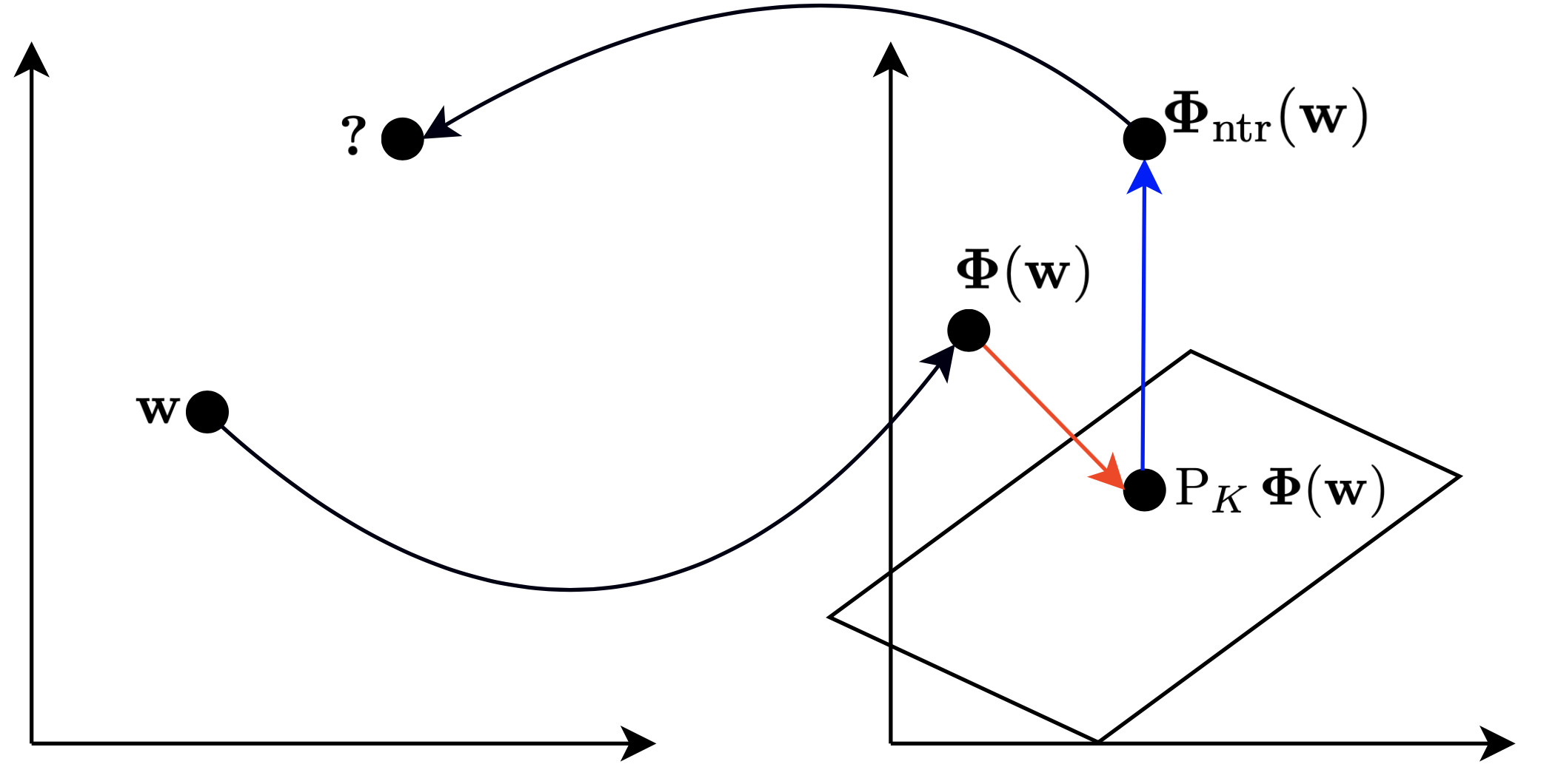
Figure 1: Pre-image problem illustration for the neutralised embeddings (null-space). The plane represents represents the bias subspace in the RKHS.

5 Computing the Pre-Image

As mentioned in the previous section, a downfall of the metric correction approach is that it does not provide us embeddings that we can use in downstream tasks: the bias-mitigated embeddings only exist in feature space. Thus, when it comes to transfer tasks such as classification we are limited to kernel methods such (i.e. support vector machines). One way to resolve this problem is by obtaining the pre-image of the corrected representations in the feature space.

Finding the pre-image is a well studied problem for kernel PCA Kwok and Tsang (2004). The goal is to fine the pre-image mappings $\Gamma:\mathcal{H}_{K}\oplus\mathcal{H}_{K}^{\perp}\rightarrow\mathbb{R}^{d}$, $\Gamma^{\perp}:\mathcal{H}_{K}^{\perp}\rightarrow\mathbb{R}^{d}$ and $\Gamma^{\top}:\mathcal{H}_{K}\rightarrow\mathbb{R}^{d}$ that compute (or approximate) the pre-images for ${\bm{\Phi}}(\mathbf{w}_{i}),{\bm{\Phi}}_{\operatorname{P}_{K}}^{\perp}(\mathbf{w}_{i})$ and ${\bm{\Phi}}_{\operatorname{P}_{K}}(\mathbf{w}_{i})$, respectively. In our case, with the pre-image maping, the neutralize step from Bolukbasi et al. (2016) becomes

$$\mathbf{z}_{i}^{\star}=\Gamma^{\perp}\left({\bm{\Phi}}(\mathbf{w}_{i})-\operatorname{P}_{K}{\bm{\Phi}}(\mathbf{w}_{i})\right)$$ (21)

In general, we will not have access to $\Gamma^{\perp}$ so we discuss the following approximation scheme.

Additive Decomposition Approach.

Alternatively, following Kandasamy and Yu (2016), we can construct an approximation to $\Gamma$ that additively decomposes over the direct sum $\oplus$. We decompose $\Gamma$ additively over the direct sum $\mathcal{H}_{K}\oplus\mathcal{H}_{K}^{\perp}$. That is, we assume that the pre-image mappings have the following form:

kernel	$\kappa(\mathbf{w}_{i},\mathbf{w}_{j})$
Cosine	$\frac{\mathbf{w}_{i}^{\top}\mathbf{w}_{j}}{||\mathbf{w}_{i}||_{2}\,||\mathbf{w}_{j}||_{2}}$
RBF Kernel	$\exp\left(-\gamma\,||\mathbf{w}_{i}-\mathbf{w}_{j}||_{2}^{2}\right)$
Sigmoid Kernel	$\tanh(\gamma\,\mathbf{w}_{i}^{\top}\mathbf{w}_{j}+c_{0})$
Polynomial Kernel	$(\gamma\,\mathbf{w}_{i}^{\top}\mathbf{w}_{j}+c_{0})^{d}$
Laplace Kernel	$\exp(-\gamma\,||\mathbf{w}_{i}-\mathbf{w}_{j}||_{1})$
Convex Combination	$\sum_{\ell=1}^{L}\alpha_{\ell}\,\kappa_{n}(\mathbf{w}_{i},\mathbf{w}_{j}),$

Table 1: Different kernels used throughout experiments.

Targets	Original		PCA		KPCA (rbf)		KPCA (sig)		KPCPA (lap)
	d	p	d	p	d	p	d	p	d	p
Google News Word2Vec Mikolov et al. (2013)
Career , Family	1.622	0.000	1.327	0.001	1.321	0.005	1.319	0.006	1.311	0.002
Math, Arts	0.998	0.017	-0.540	0.859	-0.755	0.922	-0.754	0.933	-0.024	0.507
Science , Arts	1.159	0.005	0.288	0.281	0.271	0.307	0.269	0.283	1.110	0.009
GloVe Pennington et al. (2014)
Career , Family	1.749	0.000	1.160	0.007	1.166	0.006	1.165	0.01	1.443	0.000
Math, Arts	1.162	0.007	0.144	0.389	0.096	0.437	0.095	0.411	0.999	0.015
Science , Arts	1.281	0.008	-1.074	0.985	-1.114	0.995	-1.112	0.993	-0.522	0.839

Table 2: WEAT results using GloVe and Google News word embeddings.

$$\Gamma({\bm{\Phi}}(\mathbf{w})) =\Gamma^{\perp}\left({\bm{\Phi}}_{\operatorname{P}_{K}}^{\perp}(\mathbf{w})\right)+\Gamma^{\top}({\bm{\Phi}}_{\operatorname{P}_{K}}(\mathbf{w}))$$

$$\Gamma^{\perp}\left({\bm{\Phi}}_{\operatorname{P}_{K}}^{\perp}(\mathbf{w})\right) =\Gamma({\bm{\Phi}}(\mathbf{w}))-\Gamma^{\top}({\bm{\Phi}}_{\operatorname{P}_{K}}(\mathbf{w}))$$

Given that we will always know that the pre-image of $\Gamma({\bm{\Phi}}(\mathbf{w}))$ exists and is $\mathbf{w}$, we can select $\Gamma$ to return $\mathbf{w}$ resulting in:

$$\Gamma^{\perp}\left({\bm{\Phi}}_{\operatorname{P}_{k}}^{\perp}(\mathbf{w})\right)=\mathbf{w}-\Gamma^{\top}({\bm{\Phi}}^{\top}(\mathbf{w}))$$ (22)

We then learn an analytic approximation for $\Gamma^{\top}$ using the method in Bakır et al. (2004).

Dataset Bolukbasi et al. (2016) PCA d p d p Google News Word2Vec Mikolov et al. (2013) Career , Family 1.299 0.003 1.327 0.001 Math, Arts -1.173 0.995 -0.540 0.859 Science , Arts -0.509 0.832 0.288 0.281              GloVe Pennington et al. (2014) Career , Family 1.160 0.000 1.160 0.007 Math, Arts -0.632 0.887 0.144 0.389 Science , Arts 0.937 0.937 -1.074 0.985

Table 3: Effect of the equalize step

Note that most pre-imaging methods, e.g., Mika et al. (1999) and Bakır et al. (2004), are designed to approximate a pre-image $\Gamma^{\top}$ and do not generalize to approximating the pre-image mappings $\Gamma$ and $\Gamma^{\perp}$. This is because such methods explicitly optimise for pre-imaging representations in the space $\Gamma^{\top}$ using points in the training set as examples of their pre-image, for the null-space $\Gamma^{\perp}$ we have no such examples.

6 Experiments and Results

We carry out experiments across a range of benchmarks and statistical tests designed to quantify the underlying bias in word embeddings Gonen and Goldberg (2019). Our experiments focus on quantifying both direct and indirect bias as defined in Gonen and Goldberg (2019); Hall Maudslay et al. (2019). Furthermore we also carry out word similarity experiments using the Hill et al. (2015) benchmark in order to asses that our new debiased spaces still preserve the original properties of word embeddings Mikolov et al. (2013).

6.1 Experimental Setup

Across all experiments we apply the neutralize metric correction step to all word embeddings, in contrast to Bolukbasi et al. (2016) where the equalize step is applied to the equality sets $\mathcal{E}$ and the neutralize step to a set of neutral words as determined in Bolukbasi et al. (2016). We show in Tab. 3 that applying the equalize step does not bring an enhancement over neutralizing all words. We varied kernel hyper-parameters using a grid search and found that they had little effect on performance, as a result we used default initialisation strategies as suggested in Schölkopf et al. (1998). Unless mentioned otherwise, all experiments use the inner product correction approach introduced in § 4.4.

Figure 2: 2D toy example of non-linear component removal using Kernel PCA and the pre-image (neutralize step) described in § 5.

6.2 Kernel Variations

The main kernels used throughout experiments are specified in Tab. 1. We also explored the following compound kernels: (i) convex combinations of the Laplace, radial basis function (RBF), cosine and sigmoid kernels; (ii) convex combinations of cosine similarity, RBF, and sigmoid kernels; (iii) convex combinations of RBF and sigmoid kernels; (iv) polynomial kernels up to 4${}^{\text{th}}$ degree. We only report the results on the most fundamental kernels out of the explored kernels.

6.3 Direct Bias: WEAT

The Word Embeddings Association Test Caliskan et al. (WEAT; 2017) is a statistical test analogous to the implicit association test (IAT) for quantifying human biases in textual data (Greenwald and Banaji, 1995). WEAT computes the difference in relative cosine similarity between two sets of target words $X$ and $Y$ (e.g. careers and family) and two sets of attribute words $A$ and $B$ (e.g. male names and female names). Formally, this quantity is Cohen's $d$-measure Cohen (1992) also known as the effect size: The higher the measure, the more biased the embeddings. To quantify the significance of the estimated $d$, Caliskan et al. (2017) define the null-hypothesis that there is no difference between the two sets of target words and the sets of attribute words in terms of their relative similarities (i.e. $d=0$). Using this null hypothesis, Caliskan et al. (2017) then carry out a one-sided hypothesis test where failure to reject the null-hypothesis $(p>0.05)$ means that the degree of bias measured by $d$ is not significant.

We obtain WEAT scores across different kernels (Tab. 2). We observe that the differences between the linear and the non-linear kernels is small and, in most cases, the linear kernel has a smaller value for the effect size indicating a lesser degree of bias in the corrected space. Overall, we conclude that the non-linear kernels do not reduce the linear bias as measured by WEAT further than the linear kernels. We also experiment with polynomial kernels and obtain similar results, which can be found in Tab. 7 of App. A.

6.4 Professions Gonen and Goldberg (2019)

We consider the professions dataset introduced by Bolukbasi et al. (2016) and apply the benchmark defined in Gonen and Goldberg (2019). We find the neighbors (100 nearest neighbors) of each word using the corrected cosine similarity and count the number of male neighbors. We then report the Pearson correlation coefficient between the number of male neighbors for each word and the original bias of that word. The original bias of a word vector $\mathbf{w}$ is given by the cosine similarity $\cos(\mathbf{w},\textbf{{he}}-\textbf{{she}})$ in the original word embedding space. We can observe from the results in Tab. 4 that the non-linear kernels yield only marginally different results which in most cases seem to be slightly worse, i.e. their induced space exhibits marginally higher correlations with the original biased vector space.

Embeddings Original PCA KPCA(rbf) KPCA(sig) KPCA(lap) Word2Vec 0.740 0.675 0.678 0.675 0.708 Glove 0.758 0.675 0.681 0.680 0.715

Table 4: Pearson correlation coefficients of professions analogy task. All observed at significant at $\alpha=0.05$. Indeed, all have $p$-values $<10^{-30}$.

Embeddings Original PCA KPCA(rbf) KPCA(sig) KPCA(lap) Word2Vec 0.974 0.702 0.716 0.715 0.720 Glove 0.978 0.757 0.754 0.753 0.914

Table 5: Classification accuracy results on male versus female terms.

6.5 Indirect Bias

Following Gonen and Goldberg (2019), we build a balanced training set of male and female words using the 5000 most biased words according to the bias in the original embeddings as described in Section 6.4, and then train an RBF-kernel support vector machine (SVM) classifier Pedregosa et al. (2011) on a random sample of 1000 (training set) of them to predict the gender, and evaluate its generalization on the remaining 4000 (test set). We can perform classification in our corrected RKHS with any SVM kernel $\kappa_{\mathrm{svm}}({{\bm{\Phi}}_{\mathrm{ntr}}}(\mathbf{w}),{{\bm{\Phi}}_{\mathrm{ntr}}}(\mathbf{z}))$ that can be written in the forms $\kappa_{\mathrm{svm}}(\langle\mathbf{w},\mathbf{z}\rangle)$ or $\kappa_{\mathrm{svm}}(||\mathbf{w}-\mathbf{z}||^{2})$ since we can use the kernel trick in our corrected RKHS $\langle{{\bm{\Phi}}_{\mathrm{ntr}}}(\mathbf{w}),{{\bm{\Phi}}_{\mathrm{ntr}}}(\mathbf{z})\rangle=\tilde{\kappa}(\mathbf{w},\mathbf{z})$ to compute the inputs to our SVM kernel, resulting in

$$\kappa_{\mathrm{svm}} (||\mathbf{w}-\mathbf{z}||^{2})$$ (23)

$$=\kappa_{\mathrm{svm}}(\tilde{\kappa}(\mathbf{w},\mathbf{w})-2\tilde{\kappa}(\mathbf{w},\mathbf{z})+\tilde{\kappa}(\mathbf{z},\mathbf{z})).$$

It is clear that the RBF kernel is an example of a kernel that follows Eq. 23.

We can see that the bias removal induced by non-linear kernels results in a slightly higher classification accuracy (shown in Tab. 5) of gendered words for GoogleNews Word2Vec embeddings Mikolov et al. (2013) and a slightly lower classification accuracy for GloVe embeddings Pennington et al. (2014) (with the exception of the Laplace kernel which has a very high classification accuracy). Overall for the RBF and the sigmoid kernels there is no improvement in comparison to the linear kernel (PCA), the Laplace kernel seems to have notably worse results than the others, still being able to classify gendered words at a high accuracy of 91.4% for GloVe embeddings.

6.6 Word Similarity: SimLex-999

The quality of a word vector space is traditionally measured by how well it replicates human judgments of word similarity. We use the SimLex-999 benchmark by Hill et al. (2015) which provides a ground-truth measure of similarity produced by 500 native English speakers. Similarity scores by our method are computed using Spearman correlation between embedding and human judgments are reported. We can observe that the metric corrections only slightly change the Spearman correlation results on SimLex-999 (Tab. 6) from the original embedding space. We can thus conclude that the embedding quality is mostly preserved.

Embeddings Original PCA KPCA(rbf) KPCA(sig) KPCA(lap) Word2Vec 0.121 0.119 0.118 0.118 0.118 Glove 0.302 0.298 0.298 0.298 0.305

Table 6: Correlation on SimLex-999 using GoogleNews Word2Vec and GloVe embeddings. The significance level is $\alpha=0.05$ with $p<0.001$.

7 Conclusion

We offer a non-linear extension to the method presented in Bolukbasi et al. (2016) by connecting its bias space construction to PCA and subsequently applying kernel PCA. We contend our extension is natural in the sense that it reduces to the method of Bolukbasi et al. (2016) in the special case when we employ a linear kernel and in the non-linear case it preserves all the desired linear properties in the feature space. This allows us to provide equivalent constructions of the neutralize and equalize steps presented.

We compare the linear bias mitigation technique to our new kernelized non-linear version across a suite of tasks and datasets. We observe that our non-linear extensions of Bolukbasi et al. (2016) show no notable performance differences across a set of benchmarks designed to quantify gender bias in word embeddings. Furthermore, the results in Tab. 7(App. A) show that gradually increasing the degree of non-linearity has again no significant change in performance for the WEAT Caliskan et al. (2017) benchmark. Thus, we provide empirical evidence for the linear subspace hypothesis; our results suggest representing gender bias as a linear subspace is a suitable assumption. We would like to highlight that our results are specific to our proposed kernelized extensions and does not imply that all non-linear variants of Bolukbasi et al. (2016) will yield similar results. There may very well exist a non-linear technique that works better, but we were unable to find one in this work.

8 Acknowledgements

We would like to thank Jennifer C. White for amending several typographical errors in final version of this manuscript.

Targets	Original		PCA		KPCA (poly-2)		KPCA (poly-3)		KPCPA (poly-4)
	d	p	d	p	d	p	d	p	d	p
Google News Word2Vec Mikolov et al. (2013)
Career , Family	1.622	0.000	1.327	0.001	1.320	0.004	1.321	0.001	1.312	0.002
Math, Arts	0.998	0.017	-0.540	0.859	-0.755	0.927	-0.755	0.933	-0.754	0.932
Science , Arts	1.159	0.005	0.288	0.281	0.271	0.312	0.272	0.305	0.272	305
GloVe Pennington et al. (2014)
Career , Family	1.749	0.000	1.160	0.007	1.166	0.000	1.166	0.009	1.667	0.005
Math, Arts	1.162	0.007	0.144	0.389	0.096	0.429	0.097	0.421	0.097	0.432
Science , Arts	1.281	0.008	-1.074	0.985	-1.113	0.995	-1.114	0.994	-1.114	0.992

Table 7: Results for polynomial Kernel Experiments on Glove and Google News embeddings.

Appendix A Polynomial Kernel Results

For experimental completeness, we provide direct bias experiments on WEAT using a range of polynomial kernels. The results are displayed in Tab. 7. The results for the polynomial kernels suggest the same conclusions we arrived at in the main text, i.e. a linear kernel is generally enough.

References

- Bakır et al. (2004) Gökhan H. Bakır, Jason Weston, and Bernhard Schölkopf. 2004. Learning to find pre-images. Advances in Neural Information Processing Systems, 16:449–456.
- Bolukbasi et al. (2016) Tolga Bolukbasi, Kai-Wei Chang, James Y. Zou, Venkatesh Saligrama, and Adam T. Kalai. 2016. Man is to computer programmer as woman is to homemaker? Debiasing word embeddings. In Advances in Neural Information Processing Systems, pages 4349–4357.
- Caliskan et al. (2017) Aylin Caliskan, Joanna J. Bryson, and Arvind Narayanan. 2017. Semantics derived automatically from language corpora contain human-like biases. Science, 356(6334):183–186.
- Cohen (1992) Jacob Cohen. 1992. Statistical power analysis. Current Directions in Psychological Science, 1(3):98–101.
- Devlin et al. (2019) Jacob Devlin, Ming-Wei Chang, Kenton Lee, and Kristina Toutanova. 2019. BERT: Pre-training of deep bidirectional transformers for language understanding. In Proceedings of the 2019 Conference of the North American Chapter of the Association for Computational Linguistics: Human Language Technologies, Volume 1 (Long and Short Papers), pages 4171–4186, Minneapolis, Minnesota. Association for Computational Linguistics.
- Goldberg (2017) Yoav Goldberg. 2017. Neural Network Methods in Natural Language Processing. Morgan & Claypool Publishers.
- Gonen and Goldberg (2019) Hila Gonen and Yoav Goldberg. 2019. Lipstick on a pig: Debiasing methods cover up systematic gender biases in word embeddings but do not remove them. In Proceedings of the 2019 Conference of the North American Chapter of the Association for Computational Linguistics: Human Language Technologies, Volume 1 (Long and Short Papers), pages 609–614, Minneapolis, Minnesota. Association for Computational Linguistics.
- Greenwald and Banaji (1995) Anthony G. Greenwald and Mahzarin R. Banaji. 1995. Implicit social cognition: Attitudes, self-esteem, and stereotypes. Psychological Review, 102(1):4.
- Hall Maudslay et al. (2019) Rowan Hall Maudslay, Hila Gonen, Ryan Cotterell, and Simone Teufel. 2019. It's all in the name: Mitigating gender bias with name-based counterfactual data substitution. In Proceedings of the 2019 Conference on Empirical Methods in Natural Language Processing and the 9th International Joint Conference on Natural Language Processing (EMNLP-IJCNLP), pages 5266–5274, Hong Kong, China. Association for Computational Linguistics.
- Hill et al. (2015) Felix Hill, Roi Reichart, and Anna Korhonen. 2015. Simlex-999: Evaluating semantic models with (genuine) similarity estimation. Computational Linguistics, 41(4):665–695.
- Kandasamy and Yu (2016) Kirthevasan Kandasamy and Yaoliang Yu. 2016. Additive approximations in high dimensional nonparametric regression via the SALSA. In International Conference on Machine Learning, pages 69–78.
- Karve et al. (2019) Saket Karve, Lyle Ungar, and João Sedoc. 2019. Conceptor debiasing of word representations evaluated on WEAT. arXiv preprint arXiv:1906.05993.
- Kwok and Tsang (2004) James T. Kwok and Ivor W. Tsang. 2004. The pre-image problem in kernel methods. IEEE Transactions on Neural Networks, 15(6):1517–1525.
- May et al. (2019) Chandler May, Alex Wang, Shikha Bordia, Samuel R. Bowman, and Rachel Rudinger. 2019. On measuring social biases in sentence encoders. In Proceedings of the 2019 Conference of the North American Chapter of the Association for Computational Linguistics: Human Language Technologies, Volume 1 (Long and Short Papers), pages 622–628, Minneapolis, Minnesota. Association for Computational Linguistics.
- Mika et al. (1999) Sebastian Mika, Bernhard Schölkopf, Alex J. Smola, Klaus-Robert Müller, Matthias Scholz, and Gunnar Rätsch. 1999. Kernel PCA and de-noising in feature spaces. In Advances in Neural Information Processing Systems, pages 536–542.
- Mikolov et al. (2013) Tomas Mikolov, Kai Chen, Greg Corrado, and Jeffrey Dean. 2013. Efficient estimation of word representations in vector space. arXiv preprint arXiv:1301.3781.
- Pedregosa et al. (2011) F. Pedregosa, G. Varoquaux, A. Gramfort, V. Michel, B. Thirion, O. Grisel, M. Blondel, P. Prettenhofer, R. Weiss, V. Dubourg, J. Vanderplas, A. Passos, D. Cournapeau, M. Brucher, M. Perrot, and E. Duchesnay. 2011. Scikit-learn: Machine Learning in Python . Journal of Machine Learning Research, 12:2825–2830.
- Pennington et al. (2014) Jeffrey Pennington, Richard Socher, and Christopher Manning. 2014. Glove: Global vectors for word representation. In Proceedings of the 2014 Conference on Empirical Methods in Natural Language Processing (EMNLP), pages 1532–1543, Doha, Qatar. Association for Computational Linguistics.
- Peters et al. (2018) Matthew Peters, Mark Neumann, Mohit Iyyer, Matt Gardner, Christopher Clark, Kenton Lee, and Luke Zettlemoyer. 2018. Deep contextualized word representations. In Proceedings of the 2018 Conference of the North American Chapter of the Association for Computational Linguistics: Human Language Technologies, Volume 1 (Long Papers), pages 2227–2237, New Orleans, Louisiana. Association for Computational Linguistics.
- Rudinger et al. (2018) Rachel Rudinger, Jason Naradowsky, Brian Leonard, and Benjamin Van Durme. 2018. Gender bias in coreference resolution. In Proceedings of the 2018 Conference of the North American Chapter of the Association for Computational Linguistics: Human Language Technologies, Volume 2 (Short Papers), pages 8–14, New Orleans, Louisiana. Association for Computational Linguistics.
- Schölkopf et al. (1997) Bernhard Schölkopf, Alexander Smola, and Klaus-Robert Müller. 1997. Kernel principal component analysis. In International Conference on Artificial Neural Networks, pages 583–588. Springer.
- Schölkopf et al. (1998) Bernhard Schölkopf, Alexander Smola, and Klaus-Robert Müller. 1998. Nonlinear component analysis as a kernel eigenvalue problem. Neural Computation, 10(5):1299–1319.
- Zhao et al. (2019) Jieyu Zhao, Tianlu Wang, Mark Yatskar, Ryan Cotterell, Vicente Ordonez, and Kai-Wei Chang. 2019. Gender bias in contextualized word embeddings. In Proceedings of the 2019 Conference of the North American Chapter of the Association for Computational Linguistics: Human Language Technologies, Volume 1 (Long and Short Papers), pages 629–634, Minneapolis, Minnesota. Association for Computational Linguistics.
- Zhao et al. (2018) Jieyu Zhao, Tianlu Wang, Mark Yatskar, Vicente Ordonez, and Kai-Wei Chang. 2018. Gender bias in coreference resolution: Evaluation and debiasing methods. In Proceedings of the 2018 Conference of the North American Chapter of the Association for Computational Linguistics: Human Language Technologies, Volume 2 (Short Papers), pages 15–20, New Orleans, Louisiana. Association for Computational Linguistics.