Lagrangian and Hamiltonian Dynamics for Probabilities on the Statistical Bundle
Abstract
We provide an Information-Geometric formulation of accelerated natural gradient on the Riemannian manifold of probability distributions, which is an affine manifold endowed with a dually-flat connection. In a non-parametric formalism, we consider the full set of positive probability functions on a finite sample space, and we provide a specific expression for the tangent and cotangent spaces over the statistical manifold, in terms of a Hilbert bundle structure that we call the Statistical Bundle. In this setting, we compute velocities and accelerations of a one-dimensional statistical model using the canonical dual pair of parallel transports and define a coherent formalism for Lagrangian and Hamiltonian mechanics on the bundle. We show how our formalism provides a consistent framework for accelerated natural gradient dynamics on the probability simplex, paving the way for direct applications in optimization.
keywords:
Information Geometry, Statistical Bundle, Kullback–Leibler Lagrangian, Accelerated Natural Gradient, Variational Approaches to Optimization Methods1 Introduction
Gradient-based optimization and its application to large-scale statistical inference problems are a very active topic in machine learning [15]. In recent years, following the milestone work of [36], accelerated gradient methods [37, 38, 39] had significant impact in optimization, given their ability to improve their convergence rate compared to gradient-based algorithms, and in certain cases to yield optimal rates [35].
Despite the large amount of work on acceleration in optimization, and the intuitive explanation that the Nesterov method can be described in terms of momentum, there is the lack of a unifying theoretical framework for the derivations of accelerated methods from a unique underlying principle. Recently, [52] addressed this issue by proposing a generative approach for accelerated methods, where accelerated optimization is recast in the form of a variational problem. In this setting, the Euler-Lagrange equations derived from a family of Bregman Lagrangians provide a continuous time analogue of the typical oracle’s gradient descent dynamics which allows to generate a large class of accelerated methods, including non-Euclidean extensions.
In statistics and machine learning, inference procedures are often characterized by the minimization of a loss function defined over parameterized statistical models, accomplished by gradient descent methods. Under common regularity conditions, statistical models admit a manifold structure [6, 9] and the optimization process often benefits by being set in a Riemannian context [2]. Indeed, the Riemannian natural gradient [8], that takes into account the metric of the space for the identification of the direction of steepest descent, has proved to provide benefits in terms of speed of convergence in optimization, compared to the plain vanilla Euclidean gradient. The generalization of accelerated methods to Riemannian manifolds has been investigated more recently by several authors, including [32, 53, 3].
In this paper, motivated by the approach developed by [52], suitable for an arbitrary Hessian metric over a convex set in , and with the general aim to inquire about the relation between the geometric mechanics and Information Geometry [18, 31, 42, 20],111The interest of dynamical systems on probability functions has raised in several areas, for example, Compartmental Models, Replicator Equations, Prey-Predator Equations, Mass Action Equations, Differential Games, beside in Optimization Methods and Machine Learning Theory. we define a theoretical framework for accelerated continuous-time dynamics over statistical manifolds, leading to the acceleration of the natural gradient. Notably, our framework defines Lagrangian and Hamiltonian mechanics of statistical manifolds, starting from generic diverge functions between probability distributions, hence including the Bregman Lagrangian as a special case.
Our construction is not limited to statistical manifolds, but it can be applied to any dually-flat geometry characterizing Hessian manifolds. Specifically, by considering functions defined over the natural parameters of the exponential family, which is a convex set by definition, together with the Fisher information matrix as a metric, we recover as a special case an instance of the framework developed in [52].
Two specific qualifications characterise our approach. Information Geometry, as firstly formalized by [9], views parametric statistical models as a manifold endowed with a Riemannian metric and a family of dual connections, the -connections. Differently, we consider the full set of positive probability functions on a finite sample space and discuss Information Geometry in the non-parametric geometric language (cf. [30, 27]). In data analysis, the non-parametric statistical study of compositional data has been started by [4]. We use here the simplest instance of non-parametric Information Geometry as it is described in the review papers by [41, 44].
The second and most qualifying choice, consists in considering Information Geometry as defined on a linear bundle, not just on a manifold of probability densities. In classical mechanics, the study of the evolution of a system requires both position and velocities , or position and conjugate momenta in the phase space description. Lagrangian and Hamiltonian mechanics are defined, respectively, on the tangent and co-tangent bundle of a finite-dimensional Riemannian manifold [10, Ch. III-IV]. Similarly, in statistics, we argue that the study of probability evolution is most naturally described by a fiber bundle structure comprising couples of probability densities and associated scores (-derivatives), or equivalently by densities and score conjugate momenta . We call such a bundle the Statistical Bundle [42]. This idea should be compared with the use of the Grassmannian manifold, as defined, for example in [2], to describe the various centering of the space of the sufficient statistics of an exponential family [33, 34].
In the case of strictly positive densities, the affine geometry of the Statistical Bundle is fully characterised by an affine atlas and a couple of dual parallel transports. With that, one easily computes the form of all the relevant second-order quantities which are necessary to define a notion of acceleration for in the space of probability densities.
In this setting, first order differential equations are confirmed to correspond to replicator equations, as discussed, for example, in [12, §6.2]. However, we are able to show that also the second-order Euler-Lagrange equation (as well as the Hamiltonian equation) can be expressed as a system of replicator equations. In this sense, the statistical bundle framework provides a possible solution to the problem of second-order evolution equation on the simplex, which has been raised in the optimization literature.
The paper is organised as follows. In section 2, we introduce the non-parametric description of the statistical bundle and the maximal exponential family. We define a convenient full bundle extension for this structure, which carries tuples of both exponential and mixture fibers at each point. In section 3, we recall the main features of the Hessian geometry of the maximal exponential family. We focus on the second-order geometry, introducing consistent notions of velocity, covariant derivative, and acceleration on higher order statistical bundles. In section 4, we generalize the computation of the natural gradient to the Lagrangian and the Hamiltonian function on the full bundle. Therefore, in section 5, we gathered all the necessary structure to define a mechanics of the probability simplex. We define an action integral in terms of a generic notion on Lagrangian function on the statistical bundle. We can then derive the Euler-Lagrange equation via a standard variational approach on the simplex [42]. We define a Legendre transform, hence we derive the Hamilton equations. As a starting point for our analysis, we look at the dynamics induced by a standard, though local here, particle Lagrangian obtained from the quadratic form on the statistical bundle, where the role of the point particle is played by a probability density as a point on the statistical manifold. We take the quadratic particle Lagrangian as a quadratic approximation of a Kullback-Leibler (KL) divergence function. We focus on the formal construction of a Lagrangian function from a divergence and we setup the study of the dynamics induced by a family of parameterised KL divergence Lagrangians. Finally, motivated by our interest in applications in optimization, in section 6 we consider the case of a time-dependent damped extensions of the KL Lagrangian and we apply the Lagrange-Hamilton duality to provide a first realization on the statistical bundle of the variational approach to accelerated optimisation methods recently proposed in [52]. We end with a brief discussion in section 7. In the appendices we include examples, comments, and additional derivations. Therein, we provide the full analytic solution of the geodesic motion for the free quadratic Lagrangian, complete examples of both quadratic and KL Lagrangian and Hamiltonian flows on the bundle, as well as the explicit expressions of the ODEs systems associated to the dynamics derived in section 5 and section 6.
2 Statistical Bundle
We work on a finite sample space , with . However, we are careful in using a general language that could be used in the study of an infinite or continous state space. Probabilities on a finite sample space can be presented as probability functions, that is real non-negative vectors whose components sum to 1, . In this presentation, the uniform probability function is , , . The set of all probability functions is the probability simplex , which is also described as the convex set in generated by the Dirac functions , . In this paper, we focus on strictly positive probability functions, that is our base set is the relative interior of the probability simplex. A random variable is a real function on and its expected value with respect to the probability function is . Equivalently, a probability function on is described by its density with respect to the uniform probability function, . A random variable is centered with respect to if .
Given a probability density , we shall look systematically to a random variable as the sum of its -mean value and the fluctuation . We define the entropy function to be , so that the entropy of the uniform probability density is 0. The Kullback-Leibler divergence is , so that . We represent the open probability simplex as the maximal exponential family in the sense that each strictly positive probability density can be written in exponential form as , where is identified up to a constant. Uniqueness of the exponent can be obtained in at least two ways, both relevant for our construction. For each given reference density , considered as a reference state, one can write either
| (1) |
where is a constraint and the normalising constant becomes , or
| (2) |
where is a constraint and the normalizing constant becomes .
In the first case (1), the set of all possible ’s is the vector space of -centered random variables and the inverse mapping provides a chart of . In the second case (2), the co-domain for the mapping is not a vector space. Notice the equalities and .
The statistical bundle with base is
| (3) |
The bundle projection is . The mapping , uniquely defined by eq. 2, provides a section of the statistical bundle. Each fiber is the vector space of fluctuations with respect to . The statistical bundle is designed to allow for the discussion of the time evolution of curves in a space of states involving both probability distributions and fluctuations.
The statistical bundle is a semi-algebraic subset of , namely the open subset of the -Grassmannian defined by
In the following, we will retain the manifold structure induced by and proceed by adding further structure.
It will be useful to distinguish between the exponential (statistical) bundle and the mixture (statistical) bundle denoted by and introduce a duality pairing. The two bundles are algebraically equal, but they will carry different affine geometries. The duality pairing is defined on each fiber at by
| (4) |
We will consider a mixture chart defined on by . The exponential chart previously defined requires positive densities, while the mixture chart is in fact defined on all random variable whose sum of values equal 1, without any restriction on the sign. The relevance of the joint consideration of the two types of chart is shown by the following computation. If is represented by and by , it holds
The geometry of statistical models is frequently identified with a Riemannian geometry whose metric is given by the so-called Fisher metric. Such a Riemannian metric is derived either from the Hessian matrix of the log-likelihood of the model or, in a non parametric way, from the metric of the unit sphere via a square root embedding [9]. We discuss here the relation of this approach to our construction of statistical manifold.
Consider the positive quadrant of the sphere of radius 2 of and its tangent bundle . An element in the bundle is characterised by the equations , , . In this finite case, the set of positive probability densities is a convex subset of . An element of the tangent bundle is characterised by the equations , , . The tangent mapping of the so-called square embedding identifies the two bundles:
| (5) |
The inverse transformation is so that the inner product of restricted to the fiber is pushed forward to the (trivial) fiber , , as
that is, the Fisher metric. If we now move from the statistical bundle to the tangent bundle by the trivialization mapping
| (6) |
the push forward of the Fisher metric to is
that is, the restriction of the inner product of . In conclusion, the same metric structure has three different canonical expressions, according to the choice of the bundle among isomorphic expressions,
Our choice of the statistical bundle as basic representation is motivated by two arguments. First, the representation on the sphere produces results that do not have a clear statistical interpretation. Second, the description of the affine connections is especially simple in the statistical bundle.
Let us discuss briefly the issue of the parameterization of the statistical bundle. For the purpose of doing computations, it could be convenient to represent probabilities as probability functions in the open probability simplex instead of probability densities with respect to the uniform probability. Moreover, one could restrict to the set of probabilities defined by parameters , . In this presentation the tangent space is the space . A straightforward computation shows that the Fisher metric is represented in the standard basis by the matrix .
We now proceed to introduce the affine geometry of the statistical bundle. Recall that we look at the inner product on the fibers as a duality pairing between and . This point of view allows for a natural definition of a dual covariant structure. Namely, we define two affine transports among the fibers of each of the statistical bundles. See the parametric version in [9] and the first non-parametric version in [23].
For each random variable , it holds
| (7) |
so that both and belong to . This prompts for the following definition.
Definition 2.1.
The exponential transport is defined for each by
| (8) |
while the mixture transport is
| (9) |
The e-transport and the m-trasport are semi-groups of affine transformations which are compatible with the statistical bundle and are dual of each other with respect to the scalar product on each fiber. In particular, we have and , respectively.
The following properties are easily proved by applying the semi-group property of the transports and the definition of pairing .
Proposition 2.2.
The two transports defined above are conjugate with respect to the duality pairing,
| (10) |
Moreover, it holds
| (11) |
We now use these notions of transport to define a special affine atlas of charts, which will then be used to introduce the affine manifold structure providing the set-up of Information Geometry in this setting [44].
Definition 2.3.
The exponential atlas of the exponential statistical bundle is the collection of charts given for each by
| (12) |
where
| (13) |
As , we say that is the chart centered at . If , from eq. 13 follows the exponential form of as a density with respect to , namely . As , then , so that the cumulant function is defined on by
| (14) |
that is, is the expression in the chart at of Kullback-Leibler divergence of , and we can write
| (15) |
In conclusion, the patch centered at is
| (16) |
In statistical terms, the random variable is the relative point-wise information about relative to the reference , while is the deviation from its mean value at .
The expression of the other divergence in the chart centered at is
| (17) |
Definition 2.4.
The dual atlas of the mixture statistical bundle is the collection of charts given for each by
| (18) |
We say that is the chart centered at . The patch centered at is
| (19) |
we will see that the affine structure is defined by the affine atlases.
Remark 2.5.
As an aside, we underline that there is a further structure of interest, namely the Hilbert bundle. This is obtained by considering each fiber as an expression of the tangent bundle and taking the inner product as a Riemannian metric. In this case, the relevant Levi-Civita connection associated to the metric induces a parallel transport and a geometry on the bundle which is not affine in our sense. The push forward of the Riemannian parallel transport can be computed explicitly so to have the isometric property [44]. The notion of Hilbert bundle was introduced originally by [29] and developed by [7] as a general set-up for the study of sub-models. See also the discussion in the monograph by [26, § 10.1-2]. We will not make any use of this in the following.
In some cases, especially in discussing higher-order geometry, we will need bundles whose fibers are the product of multiple copies of the mixture and exponential fibers. As a first example, the full bundle is
In general, will denote mixture factors and exponential factors. Note and .
3 Hessian Structure and Second-Order Geometry
In the construction of the statistical bundle given above, we were inspired by the original Amari’s Information Geometry [9] in that we have shown that the statistical bundle is an extension of the tangent bundle of the Riemannian manifold whose metric is the Fisher metric and, moreover, we have provided a system of dually affine parallel transports. In this section, we proceed by introducing a further structure, namely, we show that the base manifold is actually a Hessian manifold with respect to any of the convex functions , , see [47]. Many useful computations in classical Statistical Physics and, later, in Mathematical Statistics, have been actually performed using the derivatives of a master convex function, that is, using the Hessian structure.
The connection is established by the fact that the -th differential of at in the direction , given by the -linear continuous form applied to , is the -th cumulant of under the probability density , see [45, Proposition 2.4]. In particular, the following equations can be easily derived
| (20) | |||
| (21) | |||
| (22) |
For Hessian manifolds the second-order geometry gets fully encoded in the first three cumulants. In the first cumulant the directional derivative is computed by an expected value; the second cumulant defines a metric bilinear form and allows to compute inner products as covariances; the third cumulant directly relates to the computation of the covariant derivative for Hessian manifolds. With such computational tools, we can proceed to discuss the kinematics of the statistical bundles.
3.1 Velocities and Covariant Derivatives
Let us compute the expression of the velocity at time of a smooth curve
| (23) |
in the exponential chart centered at . The expression of the curve is
| (24) |
and hence we have, by denoting the ordinary derivative of a curve in by the dot,
| (25) |
and
| (26) |
There is a clear advantage in expressing the tangent at each time in the moving frame centered at the position of the curve itself. Because of that, we define the velocity of the curve
| (27) |
to be
| (28) |
It follows that is a curve in the statistical bundle whose expression in the chart centered at (the reference density in eq. 27) is . In fact,
| (29) |
The mapping is a lift of the curve to the statistical bundle.
The velocity as defined above is nothing else but the score function of a one-dimensional parametric statistical model, see, for example, the contemporary textbook by [19], §4.2.
Let us turn to the interpretation of the second component in eq. 26. Given the exponential parallel transport, we define a covariant derivative by setting
| (30) |
Throughout the paper, the notation denotes the covariant time derivative in a given transport or connection, whose choice will depend on the context.
Let us do the computation in the dual bundle. The curve now is and the expression of the second component is . This gives
| (31) |
which, in turn, gives the dual covariant derivative
| (32) |
The couple of covariant derivatives of eqs. 28 and 30 are compatible with the duality pairing, as the following proposition shows.
Proposition 3.1 (Duality of the covariant derivatives).
For each smooth curve in the full statistical bundle,
it holds
| (33) |
Proof 3.2.
The proof is a simple computation based on LABEL:{eq:transports-duality}.
Let us now look at the duality pairing as an inner product on the Hilbert space . As topological vector spaces, we can use the identification , so that we can consider the full bundle as an Hilbert bundle. Let be given a smooth curve in such a bundle, . Because now the two statistical bundles are identified, we are bound to provisionally use different notations for the two covariant derivatives.
By using the symmetry, we get
where
Up now, we have defined the following derivation operators on the statistical bundles:
-
1.
A velocity , which is the expression in the moving frame of the derivative.
-
2.
An exponential covariant derivative .
-
3.
A mixture covariant derivative, .
-
4.
A Hilbert covariant derivative
corresponding to the canonical Riemannian (or Levi-Civita) connection on the Hilbert bundle.
Remark 3.3.
We have used here a presentation based on one-dimensional statistical models. From the differential geometry point of view is more common to define covariant derivation on a vector field. We briefly comment about this issue below.
Given two smooth section of the statistical bundle, that is two differentiable mappings , such that for all it holds , the covariant derivative is defined by
A detailed discussion of the geometry associated to our setting should include, for example, the computation of the Christoffel coefficients and the curvature of each of the three connections we have introduced. Some of these computations are not really relevant for our main goal, that is, the foundations of the mechanics of the statistical bundle. Others are probably useful and interesting.
As an example, let us verify that the Hilbert connection defined above is the unique Levi-Civita connection. We shall check that the connection is torsion-free, that is , where indicates the commutator of vector fields in the Hilbert bundle modeled on the Riemannian connection of the positive sphere.
We have, for each and , that
The form of the Hilbert covariant derivative in terms of ordinary derivatives of fields is
It follows that the bracket is
In fact, the expectation term is zero because .
We define the second statistical bundle to be
| (34) |
with charts centered at each defined by
| (35) |
The second bundle is an expression of the tangent bundle of the exponential bundle. For each curve in the statistical bundle, we define its velocity at to be
| (36) |
because is a curve in the second statistical bundle and that its expression in the chart at has the last two components equal to the values given in eq. 25 and eq. 26, respectively. The corresponding notion of gradient will be discussed in the next section.
In particular, for each smooth curve , the velocity of its lift is
| (37) |
where the acceleration at is
| (38) |
Notice that the computations above are performed in the embedding space.
The acceleration has been defined using the transports. Indeed, the connection here is defined by the transports , an approach that seems natural from the probabilistic point of view, cf. [23]. The non-parametric approach to Information Geometry allows to define naturally a dual transport, hence the dual connection of [9].
The acceleration defined above has the one-dimensional exponential families as (differential) geodesics. Every exponential (Gibbs) curve has velocity , so that the acceleration is . Conversely, if one writes , then
so that .
Example 3.4.
Let us discuss a representation of the acceleration that does not involve the construction of a second-order bundle. Consider the curve and its lift . From the retraction , we can define a new curve
such that .
Let us compute the velocity of .
where is a scalar. That is, and differ by a scalar, in particular,
In conclusion, the following representation of the acceleration in terms of the velocities and holds true:
| (39) |
In a chart centered at , we have , , so that . In particular, in the case of an exponential model, and , a property that is equivalent to the geodesic property .
We can also define other types of acceleration. In fact, we have three different interpretation of the lifted curve, namely, we can consider as a curve in the statistical bundle , or, a curve in the dual bundle , or, a curve in the Hilbert bundle. Each of these frameworks provides a different derivation, hence, a different acceleration.
We have already defined the exponential acceleration . Further, we can define the mixture acceleration as
| (40) |
and the Riemannian acceleration by
| (41) |
In the review papers by [41, 43], the various accelerations are used to derive the relevant Taylor formulæ and the relevant Hessians. Moreover, it is shown that the Riemannian acceleration can be derived using a family of isometric transport on the Hilbert bundle. Here, we will be mostly interested in the mechanical interpretation of the acceleration.
4 Natural Gradient
In this section we generalize the (non-parametric) natural gradient to the statistical bundles. Let us first recall the definition we are going to generalize. Given a scalar field the natural gradient is the section of the dual bundle such that for all smooth curve it holds
| (42) |
The natural gradient can be computed in some cases without recourse to the computation in charts, for example,
| (43) |
In general, the natural gradient could be expressed in charts as a function of the ordinary gradient as follows. In the generic chart at , with and , it holds
| (44) |
Therefore, the natural gradient is defined as
We use here the name of natural gradient for a computation which does not involve the Fisher matrix because of our choice of the inner product. The push forward of our definition to the tangent bundle of the simplex with the Fisher metric would indeed map our definition to the Riemannian one.
We are going to generalize the computation of the gradient to other cases are of interest, namely, the Lagrangian function, or Lagrangian field, defined on the exponential bundle , and the Hamiltonian function, or Hamiltonian field, defined on the dual bundle .
To include both cases, we derive below the generalization of natural gradient to functions defined on the full statistical bundle and possibly depending on external parameters. While this derivation is essentially trivial, nevertheless we present here a full proof in order to introduce and clarify the geometrical features of our presentation of the mechanics of the open probability simplex in the next section.
In the statistical bundles the partial derivatives are not defined, but they are defined in the trivialisations given by the affine charts. Precisely, let be given a scalar field , a domain of , and a generic smooth curve
We want to write
| (45) |
where the four components of the gradient are
Let us fix a reference density and express both the given function and the generic curve in the chart at . We can write the total derivative as
In the equation above, , with denotes the differential of with respect to the -th variable, which is intended to provide a linear operator to be represented by the appropriate dual vector, that is, the value of the proper gradient.
The last term does not require any comment and we can use the ordinary Euclidean gradient:
Let us consider together the second and the third term. This is a computation of the fiber derivative and does not involve the representation in chart. Given and , that is, , we have
where denotes the fiber derivative in , which is expressed, in turn, with the relevant gradients. The notation is possibly confusing, but consider that the inner product has is always first, followed by and that the subscript to the symbol displays which component of the full bundle is considered.
We have that
Putting together all results up now, we have proved that
To identify the first term in the total derivative above, consider the “constant” case,
so that the first term reduces to . It follows that the proper way to compute the first gradient is to consider the function on defined by
which has a natural gradient whose chart representation is precisely that first term.
We state the results obtained above in the following formal statement.
Proposition 4.1.
The total derivative eq. 45 holds true, where
-
1.
is the natural gradient of
that is, with the representation in -chart
it is defined by
-
2.
and are the fiber gradients;
-
3.
is the Euclidean gradient w.r.t. the last variable.
We have concluded the computation of the total derivative of a parametric function of the full bundle. The special cases of the Lagrangian and the Hamiltonian easily follows as a specialization. Notice that the computation of the natural gradient (1) in Proposition 4.1 is done by fixing the variables in the fibers to be translations of fixed ones.
We are going to discuss the following examples: the quadratic Lagrangian ; the cumulant Lagrangian ; conjugate cumulant Hamiltonian . Detailed computations of the relevant gradients are given in C.
5 Mechanics of the Statistical Bundle
If is a smooth curve in the exponential manifold and is its lift to the statistical bundle, the action integral of the Lagrangian is
| (46) |
In the exponential chart centered at , the curve is , the coordinates of the lift are , and the expression of the Lagrangian is
The expression of the action integral in coordinates is
| (47) |
and the Euler-Lagrange equation of eq. 47 is
By using Proposition 4.1, we obtain the intrinsic expression of the Euler-Lagrange equations in the statistical bundle.
Proposition 5.1 (The Euler-Lagrange equation).
If is an extremal of the action integral, then, with the notations of Proposition 4.1,
| (48) |
At each fixed density , and each time , the partial mapping is defined on the vector space , and its gradient mapping in the duality of is . The standard Legendre transform argument provides the intrinsic form of the Hamilton equations under the following assumption.
Assumption 5.2
We will always restrict our attention to Lagrangians such that the fiber gradient mapping at , is a 1-to-1 mapping from to . In particular, this true when the partial mappings are strictly convex for each .
In our finite dimensional context, this assumption is actually equivalent to the assumption that the fiber gradient is a diffeomorphism of the statistical bundles . This is related to the properties of regularity and hyper-regularity, cf. [1, § 3.6]. The bilinear form will always be written in this order. The Legendre transform of is defined for each of the image of , so that the Hamiltonian is
| (49) |
If a solution of Euler-Lagrange eq. 48, the curve in , where is the momentum.
Proposition 5.3 (The Hamilton equations).
The two proposition above do not require here a proof because they are standard results in classical mechanics. What is relevant here is the special intrinsic form which is obtained by the use of the covariant derivatives and the gradients of the statistical bundles.
As simple examples, one can compute the Euler-Lagrange equation and the Hamilton equation for the quadratic Lagrangian and the cumulant Lagrangian, see C. A slightly more sophisticate example is inspired by the standard free particle Lagrangian, where the role of the point particle is played by a probability density as a point on the statistical manifold [42]. The Lagrangian is written as a difference of the quadratic form and a potential function given by the negative of the entropy function . We keep the inertial mass as a parameter,
The first component of the natural gradient is easily computed and the natural gradient of the entropy is eq. 43. The Euler-Lagrangian equation is
| (52) |
which is Newton’s law, written in terms of the mixture acceleration. We express this equation as a system of ordinary differential equations for and by writing and note that . (see cf. E).
A non-quadratic, non-symmetric generalization of the kinetic energy on the simplex is realised via the Kullback-Leibler divergence. We introduce this case by first discussing the very idea of deducing a Lagrangian, or a Hamiltonian, from a divergence function.
A divergence is a smooth mapping , such that for all it holds and if, and only if, . Typically, a divergence is not symmetric, and frequently the discussion involves both the divergence and the so-called dual divergence . Every divergence can be associated to a Lagrangian by the canonical mapping:
| (53) |
where , that is, . The inverse mapping is the retraction
| (54) |
As the curve has null exponential acceleration, one could say that eq. 54 defines the exponential mapping of the exponential connection, while eq. 53 defines the so-called logarithmic mapping.
The expression in a chart centered at of the mapping of eq. 54 is affine:
| (55) |
In conclusion, the correspondence above maps every divergence into a divergence Lagrangian, and conversely,
| (56) |
Notice that, according to our assumptions on the divergence, the divergence Lagrangian defined in eq. 56 is non-negative and zero if, and only if, .
Similarly, every divergence can be associated to a Hamiltonian function on the dual bundle by the canonical mapping:
| (57) |
where . The inverse mapping is
| (58) |
The canonical example is the Kullback-Leibler divergence , with cumulant Lagrangian function . Accordingly, the dual divergence is naturally associated to the Hamiltonian function
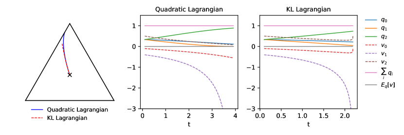
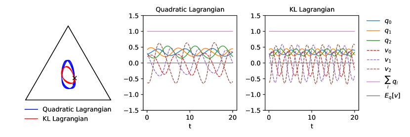
Figures 1 and 2 provide an illustration of the free motion and the motion in a potential for the quadratic and the Kullback-Leibler case.
Motivated by our interest in optimization, we will discuss now, in detail, a family of parameterized Lagrangians of the following standard form,
| (59) |
where and is a scalar field on as, for example, the negative entropy previously introduced. The Lagrangian above is parameterized in such a way that
The cumulant term is the scaled Lagrangian whose divergence function in terms of and is
| (60) |
and the limit for is null. Notice that the first term on the rhs of (60) is proportional to the -Rényi divergence of from [46].
Here, the constant is intended to introduce a mass effect in the model in such a way that implies that the Lagrangian lost any dependence on the velocity . We could talk also of an inertia of the system. Typically, the notion of inertia describes the resistance of any physical object to any change in its velocity. In our statistical setting, the dynamics of a state along some direction in the manifold can be interpreted as the result of the balance of a gain of motion, determined from the descent along some potential function (payoff), against the cost of motion to changes along a given direction from the given state. In this sense, the Lagrangian vector field on the statistical manifold consistently minimizes the action of the difference of a divergence and a potential function.
From an optimization viewpoint, our variational problem corresponds to the minimization of an objective function, the potential, with a proximity constraint enforced via the kinetic energy term. The kinetic energy acts as a regulariser for the velocities, leading to faster converging and more stable optimization algorithms [14, 22, 21].
Let us derive the Hamiltonian of our standard Lagrangian in eq. 59. If is a real function with convex conjugate , then defines a new function whose convex conjugate is , where the conjugate momentum is now a function of the parameters. In the case of a convex function, the Legendre transform coincides with the convex conjugate on the interior of the proper domain. In our case, , , and , so that
| (61) |
As , we have .
We now proceed to compute the relevant natural gradients with Proposition 4.1. By computing the total differential on the curve , we get
The Euler-Lagrange equation is
| (63) |
Let us compute the covariant time-derivative on the lhs using the trick of example 3.4. We write and recall we are using the mixture covariant derivative for . Then the left-hand side of the Euler-Lagrange equation becomes
| (64) |
where
which in turn implies
so that
The Euler-Lagrange equation becomes an equation in , , ,
or, moving the transports to the right-hand side,
| (65) |
where the right-hand side could be rewritten with . Notice that the limit form as is . For example, if , then .
A similar argument applies to the computation of the gradients of the Hamiltonian (61). The variation of on the curve is
Substitution gives
The Hamilton equations are
| (66) |
Remark 5.4.
There is a way, other than the Hamilton equations, to write a first-order system of differential equations equivalent to the second-order Euler-Lagrange eq. 65. We have found in eq. 64 that the Euler-Lagrange eq. 63 can be written as
which simplifies to
and, in turn, provides a remarkably simple system of replicator equations,
| (67) |
Notice that the vector field is null if, and only if, and .
We proceed now to express the equations we have obtained in the ordinary Euclidean space. After computing the transports in the right-hand side, the Euler-Lagrange eq. 65 becomes
| (68) |
Notice the common constant factor
in each term.
There are many ways to rewrite eq. 68 as a system of ordinary differential equations in . An immediate option is to introduce the variables and , in which case the solution will stay in the Grassmannian manifold . It holds . The acceleration is
An explicit expression for eq. 68 as a system of ordinary differential equations is given in section E.2. The solution of the ODEs system is plot in fig. 2.
The Hamiltonian equations (66) form a differential system in the two variables in the dual statistical bundle, which is an open subset of the Grassmanian manifold. The solution curve and its derivatives can be expressed in the global space in which the dual bundle is embedded by observing that and using , .
6 Application to Accelerated Optimization
As a final example of statistical Lagrangian dynamics, we consider the case of a damped mass-spring system on the probability space, defined via a time-dependent parameterized KL Lagrangian. This choice is motivated by a series of recent interesting results in optimization, where a time-dependent family of so-called Bregman Lagrangians [52] is introduced to derive a variational approach to accelerated optimization methods.
While the geometric setting in [52] is a generic Hessian manifold over a convex set in , our goal is to reproduce such a derivation on the statistical bundle, as to provide a first consistent description of accelerated optimization on the dually-flat geometry of the exponential manifold. Recent related work on the accelerated gradient flow for probability distributions can be found in [50], [51], and some relevant references therein.
6.1 Damped KL Lagrangian
On the statistical bundle, let us consider a damped Lagrangian given by the difference of time-scaled KL divergence and potential function, multiplied by an overall time-dependent damping factor,
| (69) | ||||
For each fixed , the time-dependent Lagrangian above is an instance of the standard Lagrangian eq. 59 with
which reproduces, on the statistical bundle, the time-dependent family of Bregman Lagrangians proposed in [52]. As in [52], we assume to be continuously differentiable functions of time. The overall damping factor is responsible for the dissipative behaviour of the Lagrangian system; provides the potential with an explicit time dependence; finally, defines a scaling in time of the score velocity.
In our setting, the scaling of the score is associated to a time-dependent lift to the statistical bundle. In the exponential map, we consider a time-dependent scaling of the shift vector, such that and , with smooth, open time interval. With this choice the KL divergence reads
The overall scaling by the inverse factor makes the divergence closed under time-dilation and leads to a time-reparameterization invariant [48, 16, 17] action
where we set .
It follows directly from eq. 61 that the Hamiltonian is
| (70) |
The gradients of the Lagrangian have been already computed in eq. 62,
The Euler-Lagrange equation is
or, canceling the factor ,
| (71) |
Let us compute the left-hand side. If we write , then
where
It follows that
and, in turn, the Euler-Lagrange eq. 71 becomes
The equation above can be rearranged to read
We shall now see the Euler-Lagrange equation above as the solution of an optimization problem on the simplex, where the potential represents the objective function to be minimized, with a proximity condition induced by the KL divergence. The explicit time-dependence of the Lagrangian is the fundamental ingredient in order for the dynamical system to dissipate energy and relax to a minimum of the potential, hence to a minimum of the objective function.
Remark 6.1.
In the dynamics induced by the Bregman Lagrangian analogue to eq. 69 in , [52] propose a set of ideal scaling conditions , by which solutions of the Euler-Lagrange equations reduce to vanishing-step-size-limit trajectories of the accelerated gradient optimization schemes (see also [49, 28, 11]). Applying the same ideal scaling conditions to the KL Euler-Lagrange equations on the statistical bundle leads to the simplified equation
| (72) |
Along with [52], the following choice of parameters, indexed by ,
| (73) |
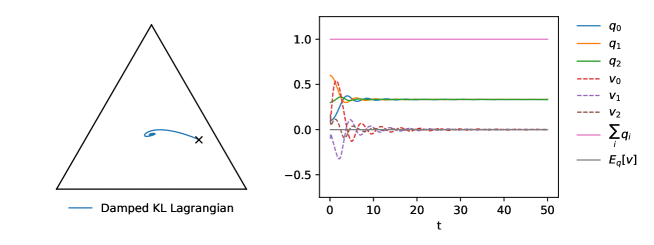
where is a constant, can be associated to the continuous-time limit of Nesterov’s accelerated mirror descent (when ) and that of Nesterov’s accelerated cubic-regularized Newton’s method (when ) on the simplex. Fig. 3 shows the solution of the system of ODEs for eq. 72. The explicit expression of the ODEs system is given in section E.3 in appendix.
6.2 Damped KL Hamiltonian
The momentum corresponding to the damped KL Lagrangian is given by
| (74) |
corresponding to a time-dependent damping of the mechanic momentum associated to the free KL Lagrangian
Now, for , we can use the exponential chart at to easily invert the Legendre transform and solve for the velocity . We have
Thereby, we can write the KL Hamiltonian as
as presented in (70).
Remark 6.2.
In classical mechanics, we normally identify the Hamiltonian with the total energy of the system, given by the sum of the kinetic and potential energy. In facts, the kinetic energy is the conjugate to the Lagrangian kinetic energy. This is apparent in the generalised case of the KL, where the symmetry of the standard quadratic form is generalised to a conjugacy relation with respect to the dual pairing. In the finite dimensional case, where the statistical bundle coincides with the dual statistical bundle, the mechanic interpretation is then preserved.
The Hamilton equations read
| (75) |
As for eq. 66, we can express the system in the global space in which the dual bundle is embedded by using , (see cf. eq. 101), section E.3 in the appendix).
Remark 6.3.
It is interesting to note that the momentum derived from the parametric Lagrangian in (69) (a generalization of the Kanai–Caldirola Lagrangian (see for example [13, 25]) is nothing but the mechanic conjugate momentum to , defined in Proposition C.5 for the undamped system, multiplied by a scaling factor . In fact, despite giving the correct equation of motion for the damped harmonic oscillator, a Lagrangian of the type has been shown to rather describe a harmonic oscillator with variable mass [24]. This is an interesting perspective to be explored for understanding the role of inertia and acceleration in the momentum approaches for optimization.
7 Discussion
This paper has the character of a first full analysis of a new formalism to be of interest in the study of the evolution of probability densities on a finite sample space. We showed that a fully non-parametric presentation of the Lagrangian and Hamiltonian dynamics can be realized on the statistical bundle. Our version of the mechanical formalism applies to a set up that is different from the standard one. Namely, it acts on that specific version of the tangent bundle of the open probability simplex that has the most natural interpretation in terms of statistical quantities.
All the underlying mechanical concepts, such as velocity, parallel transport, accelerations, second-order equations, oscillation, damping, receive a specific statistical interpretation and are, in some cases, related with non-mechanical features, such as a divergence. Several simple examples illustrate the numerical implementation and graphical illustration of the results, which are both important in statistical and machine learning applications, as well as for a deeper understanding of accelerated methods and the construction of new geometric discretization schemes for optimization algorithms (see, for example, [53, 5]).
The use of formal mechanical concepts in statistical modelling has been unusual in the applied literature, and we believe this paper could prompt for a change of perspective. On the other side, the non-parametric treatment clearly shows the relation with the modelling used in Statistical Physics that is, Boltzmann-Gibbs theory. The case of a generic exponential family is obtained by considering the vector space generated by the constant 1 and a finite set of sufficient statistics, . In this case the fibers are . The exponential transport acts properly, while the mixture transport is computed as
where is the orthogonal projection onto .
As a further direction for future research, the dynamical system induced by the Hamilton equations on the dual bundle suggests the study of the measures on the statistical bundle and their evolution. The consideration of such measures provides an interesting extension of the Bayes paradigm in that there is a probability measure on the simplex and a transition to a measure on the fiber. Future work should consider the extension of the statistical bundle mechanics to the continuous state space, which requires the definition of a proper functional set-up. One option would be to model the fibers of the statistical bundle with an exponential Orlicz space. In such a case, the fibers of the dual statistical bundle should be modeled as the pre-dual space. Many other options are available, in particular, Orlicz-Sobolev Banach spaces, or Frèchet spaces of infinitely differentiable densities. An extension to the continuous state space and to arbitrary exponential families would allow a broad application of the information geometric formalism for accelerated methods to the optimization over statistical models, in particular in large dimensions. Three examples of such applications are the optimization of functions defined over the cone of the positive definite matrices, the minimization of a loss function for the training of neural networks, and the stochastic relaxation of functions defined over the sample space.
Acknowledgements
G.C. and L.M. are supported by the DeepRiemann project, co-funded by the European Regional Development Fund and the Romanian Government through the Competitiveness Operational Programme 2014-2020, Action 1.1.4, project ID P_37_714, contract no. 136/27.09.2016, SMIS code 103321. G.P. is supported by de Castro Statistics, Collegio Carlo Alberto, Turin, Italy. He is a member of GNAMPA-INDAM.
Appendix A Covering
The mapping (5) of the positive part of the sphere to the open simplex is actually a restriction of a smooth mapping of the full sphere to whose image is the closed simplex. The unrestricted mapping provides a topological covering of the simplex. Hence, the geodesic dynamics of the sphere is naturally mapped to a dynamics of the simplex. The following example shows how this particular behaviour is expressed in our framework.
The expression in the chart centered at of the quadratic Lagrangian follows from eq. 21,
| (76) |
where and .
The two components of the natural gradient are
With , Euler-Lagrange equation is
Notice that the belongs to the fiber of the dual bundle.
Let us express this equation as a system of second-order ODEs. By recalling that here is the dual (mixture) covariant derivative, we find that
If , this is a system of 2nd order ODE,
A second option is to take as an indeterminate . It follows that
and the equation becomes
There is a closed form solution. In fact, the solution is the image of the Riemannian exponential on the sphere of radius 1 by a proper transformation.
The mapping
where is the tangent bundle of the unit sphere , is well defined, is 1-to-1 onto the positive quadrant, and preserves the respective metrics. In fact,
Notice that this is not the Amari’s embedding that maps onto .
The exponential mapping on the Riemannian manifold is given by the geodesic defined for each by
We have ,
We leave out the check it is a geodesic.
Given , let us apply the isometric transformation, and define
with
We assume that and . Let us compute the velocity and the acceleration of . It holds and
It follows that the Riemannian acceleration on the Hilbert bundle is null.
Appendix B Entropy Flow
We compute the natural gradient of the entropy by using the Hessian formalism. Notice that, by definition, .
If
| (78) |
is a smooth curve in expressed in the chart centered at , then we can write
| (79) |
where the argument of the expectation belongs to the fiber and we have expressed the expected value as a derivative by using Eq (20).
We use then the identities
| (80) | |||
| (81) | |||
| (82) |
to obtain
| (83) |
Hence, we can identify the gradient of the entropy in the statistical bundle as
| (84) |
The integral curves of the gradient flow equation
are exponential families of the form . In fact, if we write the equation in , we get the quasi-linear ODE
and, in turn,
The behaviour as and other properties follow easily [40].
Given a section , the variation of the entropy along the integral curves, , is
For example, the condition for entropy production becomes
Appendix C Simple Examples
Here, we have collected simple examples of Lagrangian and Hamiltonian dynamics of the simplex.
Example C.1 (Quadratic Lagrangian).
If , then
| (85) |
with derivative with respect to in the direction given by
which, in turn, identifies the natural gradient as .
Example C.2 (Cumulant functional).
If , then
| (86) |
Notice that last member of the equalities is the Bregman divergence of the convex function . The derivative with respect to in the direction is
The first term is
In conclusion, . The fiber gradient is easily seen to be
In the notations of Example 3.4, , we have, for example,
This example shall be of interest for us because it is connected with the KL divergence, .
Example C.3 (Conjugate cumulant functional).
The Hamiltonian
is the Legendre transform of the cumulant function ,
In particular, the fiber gradient of is which is the inverse of the fiber gradient of . Notice that is a density, and .
Let us compute the natural gradient. The expression of the Hamiltonian in the chart at is
As, for ,
the derivative of with respect to in the direction is given by
hence .
Example C.4 (Mechanics of the quadratic Lagrangian).
If , then the Legendre transform is . The gradients are
For , the Euler-Lagrange equation is
where the covariant derivative is computed in , that is, . In terms of the exponential acceleration , the Euler-Lagrange equation reads
while in terms of the Riemannian acceleration in eq. 41, it holds .
The Hamilton equations are
with the covariant derivative again computed in .
The conserved energy is
In fact, this variational problem has a closed-form solution which is the image of a geodesic (great circle) on the sphere through an isometric covering from the tangent bundle of the sphere to the statistical bundle, see appendix A. It is interesting to note that this solution is a periodic curve in the set of all densities, but consists of different sections in because it is interrupted when it touches tangentially the border of the simplex of probability densities.
Example C.5 (Mechanics of the cumulant Lagrangian).
If , then its Legendre transform is . This is an expression of the dual divergence: as with , then , namely the relative entropy dual to the cumulant.
The gradients are
The Euler-Lagrange equation is
| (87) |
The Hamilton equations are
| (88) |
The conserved energy is
Appendix D Covariant Time-Derivative of the KL Legendre Transform
We report here the explicit calculation of the covariant time derivative
derived by expressing in the p-chart, contracted with in the direction . The calculation gives an explicit example of the formalism adopted while dealing with a triple covariance. We have
We have
Hence, eventually, we get
Appendix E ODEs Systems for the Figures in the Article
We provide here the explicit ODEs expressions for the Lagrangian dynamics on the simplex derived in the main text. There are many ways to rewrite the Euler-Lagrange equations on the simplex as a system of ordinary differential equations in . An immediate option is to introduce the variables and , in which case the solution will stay in the Grassmannian manifold .
E.1 Quadratic Lagrangian Systems - Figures 1,2
Consider first the Euler-Lagrange equation for the motion of a probability density within a potential on the statistical manifold (cf. eq. 52 in the article). This is given by
| (89) |
Let us express eq. 89 as a system of ordinary differential equations for and . We write and note that implies
| (90) |
In particular, eq. 90, together with the assumption implies . Conversely, if , then .
We have
| (91) |
where the first term on the rhs is the mixture acceleration of eq. 40. Thereby, via eq. 89, we have
| (92) |
If we write the vectors and , the system of first order differential equations is
| (93) |
The case of a free-particle Lagrangian system, whose solution is pictured in fig. 1 in the article, is obtained by setting .
E.2 Kullback-Leibler Lagrangian System - Figure 2
Consider now the family of parametrised Lagrangians given in eq. 59 in the article. We have
| (94) |
where and is a scalar field on . The associated Euler-Lagrange equation reads
| (95) |
For , the acceleration can be written as
The left-hand side of eq. 68 becomes , while the right-hand side becomes
Writing the expected values as sums, we obtain a system of ordinary differential equations. The system could be further reduced to equations between independent variables by using one of the possible parametrizations of the Grassmanian manifold.
In fig. 2 in the article, we plot a solution of the Euler-Lagrangian equation for a KL Lagrangian parametrised by and . The associated ODEs is given by
| (96) |
E.3 Damped Kullback-Leibler Lagrangian/Hamiltonian Systems under Ideal-Scaling Conditions - Figures 3,4
Here, we consider the case of the Euler-Lagrange equations for the damped KL Lagrangian under ideal scaling conditions (cf. eq. 72 in the article),
| (97) |
Again, we have such that
| (98) |
from which we get
| (99) |
Then, along with [52], the choice of parameters, indexed by (, a constant)
| (100) |
leads to the ODEs system
A solutions of the Lagrangian system above (for is shown the plot in fig. 3.
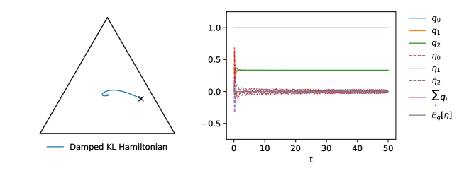
Analogously, let us consider the the damped KL Hamiltonian system (cf. eq. 75 in the article), under ideal scaling condition and with the same parametrisation given in eq. 100.
Given , we get a system of first order equations (see fig. 4)
| (101) |
A solutions of the Hamiltonian ODEs system (for ) is plot in fig. 4 in the article.
References
- [1] Ralph Abraham and Jerrold E. Marsden, Foundations of mechanics, Benjamin/Cummings Publishing Co., Inc., Advanced Book Program, Reading, Mass., 1978, Second edition, revised and enlarged, With the assistance of Tudor Raţiu and Richard Cushman. MR 515141
- [2] P.-A. Absil, R. Mahony, and R. Sepulchre, Optimization algorithms on matrix manifolds, Princeton University Press, 2008, With a foreword by Paul Van Dooren.
- [3] Kwangjun Ahn and Suvrit Sra, From nesterov’s estimate sequence to riemannian acceleration, Proceedings of Thirty Third Conference on Learning Theory (Jacob Abernethy and Shivani Agarwal, eds.), Proceedings of Machine Learning Research, vol. 125, PMLR, 09–12 Jul 2020, pp. 84–118.
- [4] J. Aitchison, The statistical analysis of compositional data, Monographs on Statistics and Applied Probability, Chapman & Hall, London, 1986. MR 865647
- [5] Foivos Alimisis, Antonio Orvieto, Gary Bécigneul, and Aurelien Lucchi, A continuous-time perspective for modeling acceleration in riemannian optimization, 2019.
- [6] Shun-ichi Amari, Differential-geometrical methods in statistics, Lecture Notes in Statistics, vol. 28, Springer-Verlag, 1985. MR 86m:62053
- [7] , Dual connections on the Hilbert bundles of statistical models, Geometrization of statistical theory (Lancaster, 1987), ULDM Publ., 1987, pp. 123–151.
- [8] Shun-Ichi Amari, Natural gradient works efficiently in learning, Neural Computation 10 (1998), no. 2, 251–276.
- [9] Shun-ichi Amari and Hiroshi Nagaoka, Methods of information geometry, American Mathematical Society, 2000, Translated from the 1993 Japanese original by Daishi Harada. MR 1 800 071
- [10] V. I. Arnold, Mathematical methods of classical mechanics, Graduate Texts in Mathematics, vol. 60, Springer-Verlag, New York, 1989, Translated from the 1974 Russian original by K. Vogtmann and A. Weinstein, Corrected reprint of the second (1989) edition. MR 1345386
- [11] Hedy Attouch, Zaki Chbani, Juan Peypouquet, and Patrick Redont, Fast convergence of inertial dynamics and algorithms with asymptotic vanishing viscosity, Mathematical Programming 168 (2018), no. 1, 123–175.
- [12] Nihat Ay, Jürgen Jost, Hông Vân Lê, and Lorenz Schwachhöfer, Information geometry, Ergebnisse der Mathematik und ihrer Grenzgebiete. 3. Folge. A Series of Modern Surveys in Mathematics [Results in Mathematics and Related Areas. 3rd Series. A Series of Modern Surveys in Mathematics], vol. 64, Springer, Cham, 2017. MR 3701408
- [13] H. Bateman, On dissipative systems and related variational principles, Phys. Rev. 38 (1931), 815–819.
- [14] Michael Betancourt, A conceptual introduction to Hamiltonian Monte Carlo, arXiv:1701.02434, 2017.
- [15] Léon Bottou, Frank E. Curtis, and Jorge Nocedal, Optimization methods for large-scale machine learning, SIAM Review 60 (2018), no. 2, 223–311.
- [16] Goffredo Chirco, Rényi relative entropy from homogeneous kullback-leibler divergence lagrangian, Geometric Science of Information (Cham) (Frank Nielsen and Frédéric Barbaresco, eds.), Springer International Publishing, 2021, pp. 744–751.
- [17] Goffredo Chirco, Thibaut Josset, and Carlo Rovelli, Statistical mechanics of reparametrization-invariant systems. It takes three to tango., Class. Quant. Grav. 33 (2016), no. 4, 045005.
- [18] Florio M. Ciaglia, Fabio Di Cosmo, Domenico Felice, Stefano Mancini, Giuseppe Marmo, and Juan M. Pérez-Pardo, Hamilton-Jacobi approach to potential functions in information geometry, Journal of Mathematical Physics 58 (2017), no. 6, 063506.
- [19] Bradley Efron and Trevor Hastie, Computer age statistical inference, Institute of Mathematical Statistics (IMS) Monographs, vol. 5, Cambridge University Press, New York, 2016, Algorithms, evidence, and data science. MR 3523956
- [20] Domenico Felice and Nihat Ay, Dynamical systems induced by canonical divergence in dually flat manifolds, 2018.
- [21] Guilherme França, Michael I. Jordan, and René Vidal, On dissipative symplectic integration with applications to gradient-based optimization, 2020.
- [22] Guilherme França, Jeremias Sulam, Daniel P. Robinson, and René Vidal, Conformal symplectic and relativistic optimization, 2019.
- [23] Paolo Gibilisco and Giovanni Pistone, Connections on non-parametric statistical manifolds by Orlicz space geometry, IDAQP 1 (1998), no. 2, 325–347. MR 1 628 177
- [24] Daniel M. Greenberger, A critique of the major approaches to damping in quantum theory, Journal of Mathematical Physics 20 (1979), no. 5, 762–770.
- [25] L. Herrera, L. Núñez, A. Patiño, and H. Rago, A variational principle and the classical and quantum mechanics of the damped harmonic oscillator, American Journal of Physics 54 (1986), 273.
- [26] Robert E. Kass and Paul W. Vos, Geometrical foundations of asymptotic inference, Wiley Series in Probability and Statistics: Probability and Statistics, John Wiley & Sons, Inc., New York, 1997, A Wiley-Interscience Publication. MR 1461540 (99b:62032)
- [27] Wilhelm P. A. Klingenberg, Riemannian geometry, second ed., De Gruyter Studies in Mathematics, vol. 1, Walter de Gruyter & Co., Berlin, 1995. MR 1330918
- [28] Walid Krichene, Alexandre Bayen, and Peter L Bartlett, Accelerated mirror descent in continuous and discrete time, Advances in Neural Information Processing Systems 28 (C. Cortes, N. D. Lawrence, D. D. Lee, M. Sugiyama, and R. Garnett, eds.), Curran Associates, Inc., 2015, pp. 2845–2853.
- [29] Masayuki Kumon and Shun-ichi Amari, Differential geometry of testing hypothesis—a higher order asymptotic theory in multi-parameter curved exponential family, J. Fac. Engrg. Univ. Tokyo Ser. B 39 (1988), no. 3, 241–273. MR 1407894
- [30] Serge Lang, Differential and Riemannian manifolds, third ed., Graduate Texts in Mathematics, vol. 160, Springer-Verlag, 1995. MR 96d:53001
- [31] Melvin Leok and Jun Zhang, Connecting information geometry and geometric mechanics, Entropy 19 (2017), no. 10, 518.
- [32] Yuanyuan Liu, Fanhua Shang, James Cheng, Hong Cheng, and Licheng Jiao, Accelerated first-order methods for geodesically convex optimization on riemannian manifolds, Proceedings of the 31st International Conference on Neural Information Processing Systems (Red Hook, NY, USA), NIPS’17, Curran Associates Inc., 2017, p. 4875–4884.
- [33] Luigi Malagò and Giovanni Pistone, Combinatorial optimization with information geometry: Newton method, Entropy 16 (2014), 4260–4289.
- [34] Mateusz Michałek, Bernd Sturmfels, Caroline Uhler, and Piotr Zwiernik, Exponential varieties, Proc. Lond. Math. Soc. (3) 112 (2016), no. 1, 27–56. MR 3458144
- [35] Arkadii Semenovich. Nemirovsky A.S. and D. B. Yudin, Problem complexity and method efficiency in optimization, Wiley,, Chichester, 1983, ”A Wiley-Interscience publication.”.
- [36] Y. Nesterov, A method for solving the convex programming problem with convergence rate , Proceedings of the USSR Academy of Sciences 269 (1983), 543–547.
- [37] Yu Nesterov, Smooth minimization of non-smooth functions, Math. Program. 103 (2005), no. 1, 127–152.
- [38] Yu. Nesterov, Gradient methods for minimizing composite objective function, LIDAM Discussion Papers CORE 2007076, Université catholique de Louvain, Center for Operations Research and Econometrics (CORE), 2007.
- [39] Yurii Nesterov, Introductory lectures on convex optimization: A basic course, 1 ed., Springer Publishing Company, Incorporated, 2014.
- [40] Giovanni Pistone, Examples of the application of nonparametric information geometry to statistical physics, Entropy 15 (2013), no. 10, 4042–4065.
- [41] , Nonparametric information geometry, Geometric science of information (Frank Nielsen and Frédéric Barbaresco, eds.), Lecture Notes in Comput. Sci., vol. 8085, Springer, Heidelberg, 2013, First International Conference, GSI 2013 Paris, France, August 28-30, 2013 Proceedings, pp. 5–36. MR 3126029
- [42] , Lagrangian function on the finite state space statistical bundle, Entropy 20 (2018), no. 2, 139.
- [43] , Information geometry of the probability simplex: A short course, NPCS (Nonlinear Phenomena in Complex Systems) 23 (2019), 221–242, arXiv:1911.01876.
- [44] , Information geometry of the probability simplex: A short course, (to appear, see arXiv:1911.01876), 2020.
- [45] Giovanni Pistone and Carlo Sempi, An infinite-dimensional geometric structure on the space of all the probability measures equivalent to a given one, Ann. Statist. 23 (1995), no. 5, 1543–1561. MR 97j:62006
- [46] Alfréd Rényi, On measures of entropy and information, Proceedings of the Fourth Berkeley Symposium on Mathematical Statistics and Probability, Volume 1: Contributions to the Theory of Statistics (Berkeley, Calif.), University of California Press, 1961, pp. 547–561.
- [47] Hirohiko Shima, The geometry of Hessian structures, World Scientific Publishing Co. Pte. Ltd., Hackensack, NJ, 2007. MR 2293045
- [48] Jean-Marie Souriau, Structure des systèmes dynamiques, Dunod, 1970, Réimpression autorisées, tirage, Èditions Jacques Gabay 2012.
- [49] Weijie Su, Stephen Boyd, and Emmanuel J. Candès, A differential equation for modeling Nesterov’s accelerated gradient method: Theory and insights, Journal of Machine Learning Research 17 (2016), no. 153, 1–43.
- [50] Amirhossein Taghvaei and Prashant Mehta, Accelerated flow for probability distributions, Proceedings of Machine Learning Research (Long Beach, California, USA) (Kamalika Chaudhuri and Ruslan Salakhutdinov, eds.), vol. 97, PMLR, 09–15 Jun 2019, pp. 6076–6085.
- [51] Yifei Wang and Wuchen Li, Accelerated information gradient flow, 2020, arXiv:1909.02102.
- [52] Andre Wibisono, Ashia C. Wilson, and Michael I. Jordan, A variational perspective on accelerated methods in optimization, Proceedings of the National Academy of Sciences 113 (2016), no. 47, E7351–E7358.
- [53] Hongyi Zhang and Suvrit Sra, Towards Riemannian accelerated gradient methods, 2018, arXiv:1806.02812.