The mass splitting in an 331-TC coupled Scenario

Abstract

The root of most of the technicolor (TC) problems lies in the way the ordinary fermions acquire their masses, where an ordinary fermion (f) couples to a technifermion (F) mediated by an Extended Technicolor (ETC) boson leading to fermion masses that vary with the ETC mass scale ($M_{E}$) as $1/M_{E}^{2}$. Recently, we discussed a new approach consisting of models where TC and QCD are coupled through a larger theory, in this case the solutions of these equations are modified compared to those of the isolated equations, and TC and QCD self-energies are of the Irregular form, which allows us to build models where ETC boson masses can be pushed to very high energies. In this work we extend these results for 331-TC models, in particular considering a coupled system of Schwinger-Dyson equations, we show that all technifermions of the model exhibit the same asymptotic behavior for TC self-energies. As an application we discuss how the mass splitting of the order $O(100)GeV$ could be generated between the second and third generation of fermions.

I Introduction

The gauge and chiral symmetry breaking in quantum field theories can be promoted by fundamental scalar bosons. However, the main ideas about symmetry breaking and spontaneous generation of fermion and gauge boson masses in field theory were based on the superconductivity theory. Nambu and Jona-LasinioNambu proposed one of the first field theoretical models where all the most important aspects of symmetry breaking and mass generation were established, as known nowadays. The possibility of spontaneous gauge and chiral symmetry breaking promoted by a composite scalar boson in the context of the Standard Model (SM) was formulated in the seventies by Weinberg we and Susskind su . The most popular version of these models was dubbed as technicolor (TC), where new fermions (or technifermions) condensate and may be responsible for the chiral and SM gauge symmetry breaking Rev1 ; Rev2 ; Rev3 .

The root of most of the TC problems lies in the way the ordinary fermions acquire their masses, where an ordinary fermion (f) couples to a technifermion (F) mediated by an Extended Technicolor (ETC) boson. These problems occur when new extended technicolor interactions (ETC) are introduced in order to provide masses to the standard quarks, leading to quark masses that vary with the ETC mass scale ($M_{E}$) as $1/M_{E}^{2}$. A likely solution of this problem was proposed by Bob Holdomholdom many years ago, remembering that TC self-energy behaves as $\Sigma_{TC}(p^{2})\approx\frac{\left\langle{\bar{F}}F\right\rangle_{\mu}}{p^{2}}\left(\frac{p}{\mu}\right)^{\gamma_{m}}$, where $\gamma_{m}$ is the mass anomalous dimension associated to the fermionic condensate.

Solutions to the above dilemma seem to require a large $\gamma_{m}$ value holdom leading to a TC self-energy with a harder momentum behavior, and many models along this idea can be found in the literature lane0 ; appel ; yamawaki ; aoki ; appelquist ; shro ; walk6 ; walk7 ; walk8 ; kura ; yama1 ; yama2 ; mira2 ; yama3 ; mira3 ; yama4 . In particular we may quote the work of Takeuchi takeuchi where the TC Schwinger-Dyson equation (SDE) was solved with the introduction of an ad hoc four-fermion interaction, which can lead to the Irregular solution for the TC self-energy, which is described by Eq.(1)

$$\Sigma_{TC}(p^{2}\rightarrow\infty)\propto\mu_{TC}[1+bg^{2}(\mu^{2}_{TC})\ln(p^{2}/\mu^{2}_{TC})]^{-\delta},$$ (1)

where $g$ is the TC running coupling constant, $b$ is the coefficient of $g^{3}$ term in the renormalization group $\beta(g)$ function and $\delta$ is a function of model parameters.

Recently we solved numerically the coupled system of the gap equations, TC (based on a $SU(2)$ group) and QCDus1 ; us2 . It turned out that both self-energies(TC and QCD) have the same asymptotic behavior of Eq.(1)(with the appropriate exchange in the respective energy scales $TC\leftrightarrow QCD$). In this work we extend the results obtained inus1 ; us2 for 331-TC model , whose structure is presented in the sequence.

In particular considering the coupled system described in Fig.(1), we show that only for the coupled system all technifermions present in the model have the same asymptotic behavior given by Eq.(1). In addition as an application we discuss how the mass splitting between the second and third generation of fermions can be generated in this model.

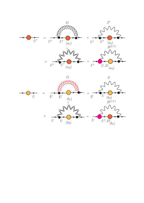
Figure 1: The coupled system of SDEs for 331-TC: In this figure (U’ $\equiv$ 1) denotes exotic techniquarks and (U $\equiv$ 2) techniquarks including ($Z^{\prime}$, $B^{(U,V)}$) and electroweak corrections. $G$ indicate technigluons interactions.

This article is organized as follows: In section 2 we present a brief review in relation to the main aspects of 331-TC models, in section 3 we discuss their coupled Schwinger-Dyson equations (SDE). In section 4 will show how the boundary conditions of the anharmonic oscillator representation of the coupled gap equation are directly related with the mass anomalous dimensions, leading to a $\gamma_{m}$ to coupled system that is compatible with a self-energy corresponding to Eq.(1). Finally, in section 5 we discuss how the mass splitting between the second and third generation of fermions can be generated , in the last section we draw our conclusions.

II $SU(N)_{{}_{TC}}\otimes SU(3)_{{}_{L}}\otimes U(1)_{{}_{X}}$ models

In some extensions of the standard model (SM), as in the so called 3-3-1 models $SU(3)_{{}_{L}}\otimes SU(3)_{{}_{c}}\otimes U(1)_{{}_{X}}$331a ; 331b ; 331c ; 331d ; 331e , new massive neutral and charged gauge bosons, $Z^{\prime}$ and $B^{(U,V)}=V^{\pm},U^{\pm\pm}$, are predicted. The 3-3-1 model is the minimal gauge group that at the leptonic level admits charged fermions and their antiparticles as members of the same multiplet, the extra predictions of these $GW=SU(2)_{{}_{L}}\otimes U(1)_{{}_{Y}}$ alternative models are leptoquark fermions with electric charges $5/3$ and $-4/3$ and bilepton gauge bosons with lepton number $L=\pm 2$. The quantization of electric charge is inevitable in the $G=3-m-1$(where m=3,4) modelsQQ1 ; QQ2 ; QQ3 ; QQ4 ; QQ5 ; QQ6 with three non-repetitive fermion generations, breaking universality independently of the character of the neutral fermions.

In the Refs.df331TC1 ; Das it was suggested that the gauge symmetry breaking of a specific version of a 3-3-1 model could be implemented dynamically, because at the scale of a few TeVs the $U(1)_{X}$ coupling constant becomes strong and the exotic quark $T$(charge $5/3$) will form a $U(1)_{X}$ condensate breaking $SU(3)_{{}_{L}}\otimes U(1)_{X}$ to the electroweak symmetry.

This possibility was explored in the Refs.df331TC2 assuming a model based on the gauge symmetry $SU(2)_{TC}\otimes SU(3)_{{}_{L}}\otimes SU(3)_{{}_{c}}\otimes U(1)_{{}_{X}}$, where the electroweak symmetry is broken dynamically by a technifermion condensate. In general TC can be characterized by the $SU(N)_{TC}$ technicolor gauge group, taking the configuration $SU(N)_{{}_{TC}}\otimes SU(3)_{{}_{L}}\otimes U(1)_{{}_{X}}$df331TC4 that we refer generically as 331-TC models.

On the lines below we describe the main features these models, the fermionic content has the following form

$$Q_{3L}=\left(\begin{array}[]{c}t\\ b\\ T\end{array}\right)_{L}\,\,\sim\,\,({\bf 1},{\bf 3},2/3)$$ (5)

$$t_{R}\,\sim\,({\bf 1},{\bf 1},2/3)\,,\,b_{R}\,\sim\,({\bf 1},{\bf 1},-1/3)$$

$$T_{R}\,\sim\,({\bf 1},{\bf 1},5/3)$$

$$Q_{\alpha L}=\left(\begin{array}[]{c}D\\ u\\ d\end{array}\right)_{\alpha L}\,\,\sim\,\,({\bf 1},{\bf 3^{*}},-1/3)$$ (9)

$$u_{\alpha R}\,\sim\,({\bf 1},{\bf 1},2/3)\,,\,d_{\alpha R}\,\sim\,({\bf 1},{\bf 1},-1/3)$$

$$D_{\alpha R}\,\sim\,({\bf 1},{\bf 1},-4/3)$$ (10)

$\alpha=1,2$ is the family index and we represent the third quark family by $Q_{3L}$. In these expressions $({\bf 1},{\bf 3},X)$, $({\bf 1},{\bf 3^{*}},X)$ or $({\bf 1},{\bf 1},X)$ denote the transformation properties under $SU(N_{TC})\otimes SU(3)_{{}_{L}}\otimes U(1)_{{}_{X}}$ and $X\equiv\frac{Y}{2}$ is the corresponding $U(1)_{X}$ charge331b ; 331c ; Das . The leptonic sector includes, besides the conventional charged leptons and their respective neutrinos, the charged heavy leptons $E_{a}$331e .

$$l_{aL}=\left(\begin{array}[]{c}\nu_{a}\\ l_{a}\\ E^{c}_{a}\end{array}\right)_{L}\,\sim\,({\bf 1},{\bf 3},0)$$ (14)

where $a=1,2,3$ is the family index and $l_{aL}$ transforms as triplets under $SU(3)_{L}$. Moreover, we have to add the corresponding right-handed components, $l_{aR}\sim({\bf 1},{\bf 1},-1)$ and $E^{c}_{aR}\sim({\bf 1},{\bf 1},+1)$.

Regarding the TC sector the fermionic has the form

$$\Psi_{1L}=\left(\begin{array}[]{c}U_{1}\\ D_{1}\\ U^{\prime}\end{array}\right)_{L}\,\,\sim\,\,({\bf N_{TC}},{\bf 3},1/2)$$ (18)

$$U_{1R}\,\sim\,({\bf N_{TC}},{\bf 1},1/2)\,,\,D_{1R}\,\sim\,({\bf N_{TC}},{\bf 1},-1/2)$$

$$U^{\prime}_{R}\,\sim\,({\bf N_{TC}},{\bf 1},3/2),$$

$$\Psi_{2L}=\left(\begin{array}[]{c}D^{\prime}\\ U_{2}\\ D_{2}\end{array}\right)_{L}\,\,\sim\,\,({\bf N_{TC}},{\bf 3^{*}},-1/2)$$ (22)

$$U_{2R}\,\sim\,({\bf N_{TC}},{\bf 1},1/2)\,,\,D_{2R}\,\sim\,({\bf N_{TC}},{\bf 1},-1/2)$$

$$D^{\prime}_{R}\,\sim\,({\bf N_{TC}},{\bf 1},-3/2),$$ (23)

the index $1$ and $2$ label the first and second techniquark families, $U^{\prime}$ and $D^{\prime}$ can be considered as exotic techniquarks making an analogy with exotic quarks $(T,D)$ that appear in the ordinary fermionic content of the model. The model is anomaly free if we have equal numbers of triplets$(3)$ and antitriplets$(3^{*})$, counting the color of $SU(3)_{c}$. Therefore, in order to make the model anomaly free two of the three quark generations transform as ${\bf 3^{*}}$, the third quark family and the three leptons generations transform as ${\bf 3}$. It is easy to check that all gauge anomalies cancel out in this model, in the TC sector the triangular anomaly cancels between the two generations of technifermions. In the present version of the model the technifermions are singlets of $SU(3)_{c}$.

III 331-TC coupled system of Schwinger-Dyson equations

The starting point in this analysis is the diagrammatic representation of the coupled SDEs for the exotic techniquarks $U^{\prime}$ and usual techniquarks $U$ self-energies, shown in the first and second lines of Fig. 1, respectively. In this figure the curly lines correspond to technigluons $(G)$ , the wavy lines to the $(Z,Z^{\prime},U,V)$ bosons and double wavy lines to fotons $(\gamma)$.

Notice that the above coupled system is rather intricate, it involves different full boson propagators and fully dressed vertices, which should be closely intertwined through the different mass scales of the theories, namely, $(\mu_{331,TC})$. Here, we restrict ourselves to exploring the result of this coupled system in a rather simplified context. Besides that, we neglect the possible contributions that the diagrams $(a_{3},b_{3})$ may give, since electromagnetic coupling constant $\alpha<\alpha_{X},\alpha_{TC}$.

In the analysis presented in this work, the conventional self-energies of the exotic techniquarks ($a_{1}$) and techniquarks ($b_{1}$) receive the perturbative corrections generated by $(Z^{\prime},U,V)$ interactions, and corrections generated by the ETC discussed in section 5. The new 3-3-1 bosons $(U,V)$ couples the exotic techniquarks to techniquarks (and vice versa), as represented by the diagrams ($a_{4}$) and ($b_{4}$).

Finally, we approximate the fully dressed propagators and vertices, entering into the gap equations, by their tree level expressions. In order to convert the system of coupled equations described in Fig. 1 into a coupled system of differential equations, we will consider the angle approximation ang , transforming terms as

$$\frac{1}{(p-k)^{2}+M^{2}}=\frac{\pi}{2}\left[\frac{\theta(p-k)}{p^{2}+M^{2}}+\frac{\theta(k-p)}{k^{2}+M^{2}}\right].$$ (24)

where $M=M_{G,Z^{\prime}}$ or $M=M_{B^{(U,V)}}$.

Moreover, we defined the notation indicated by the index $j$, where $(j=1=U^{\prime})$ and $(j=2=U)$, leading to the following TC coupled system of equations

$$\Sigma_{1}(p)=\frac{\theta_{1}}{p^{2}+m^{2}_{G}}\int^{p^{2}}_{0}dk^{2}\frac{k^{2}\Sigma_{1}(k^{2})}{k^{2}+\Sigma^{2}_{1}(k^{2})}+\theta_{1}\int^{\Lambda^{2}}_{p^{2}}dk^{2}\frac{k^{2}\Sigma_{1}(k^{2})}{k^{2}+\Sigma^{2}_{1}(k^{2})}\frac{1}{k^{2}+m^{2}_{G}}$$

$$+\frac{\theta_{Z^{\prime}}}{p^{2}+M^{2}_{Z^{\prime}}}\int^{p^{2}}_{0}dk^{2}\frac{k^{2}\Sigma_{1}(k^{2})}{k^{2}+\Sigma^{2}_{1}(k^{2})}+\theta_{Z^{\prime}}\int^{\Lambda^{2}}_{p^{2}}dk^{2}\frac{k^{2}\Sigma_{1}(k^{2})}{k^{2}+\Sigma^{2}_{1}(k^{2})}\frac{1}{k^{2}+M^{2}_{Z^{\prime}}}$$

$$+\frac{\theta_{B_{U,V}}}{p^{2}+M^{2}_{B_{U,V}}}\int^{p^{2}}_{0}dk^{2}\frac{k^{2}\Sigma_{2}(k^{2})}{k^{2}+\Sigma^{2}_{2}(k^{2})}+\theta_{B_{U,V}}\int^{\Lambda^{2}}_{p^{2}}dk^{2}\frac{k^{2}\Sigma_{2}(k^{2})}{k^{2}+\Sigma^{2}_{2}(k^{2})}\frac{1}{k^{2}+M^{2}_{B_{U,V}}}.$$

(25)

with $\theta_{j}=\frac{3C_{TC}\alpha_{TC}}{4\pi}$, $\theta_{Z^{\prime}}=\frac{3\alpha_{X}Y_{{}_{L}}Y_{{}_{R}}}{4\pi}$ and $\theta_{B_{V,U}}=\frac{3\alpha_{L}Y_{{}_{L}}Y_{{}_{R}}}{4\pi\alpha_{TC}\sqrt{2}}$. In this expressions the coupling constants $\alpha_{L}=g^{2}_{331}/4\pi$, $\alpha_{X}=g^{2}_{X}/4\pi$ are associated to the gauge group $SU(3)_{{}_{L}}\otimes U(1)_{{}_{X}}$ , and

$$\frac{\alpha_{{}_{X}}}{\alpha_{L}}=\frac{\sin^{2}\theta_{{}_{W}}(\mu)}{1-4\sin^{2}\theta_{{}_{W}}(\mu)}$$ (26)

$\theta{{}_{W}}$ is the electroweak mixing angle and $\mu=\mu_{331}$ is 331 mass scale$(\sim O(TeV))$.

The effective coupling indicated by $\theta_{B_{U,V}}$(Magenta bubble in Fig.(1)) was determined in Ref.df331TC6 . For the techniquark $U$ self-energy we have a similar equation just changing the index $1\leftrightarrow 2$, with $Z^{\prime}\to Z$ and $\theta_{Z}=\frac{3\alpha_{w}C_{w}}{4\pi}[w=weak]$.

In order to obtain the gap equation, Eq.(25), in the dimensionless form we will consider the definitions below

$$p^{2}=M^{2}_{j}x\,\,\,,\,\,\,\Sigma_{j}(p^{2})=M_{j}f_{j}(x)\,\,\,,\,\,\,\delta_{G}=\frac{m^{2}_{G}}{M^{2}_{j}}$$

$$k^{2}=M^{2}_{j}y\,\,\,,\,\,\,\Sigma_{j}(k^{2})=M_{j}f_{j}(y)\,\,\,,\,\,\,\delta_{Z,Z^{\prime},B_{U,V}}=\frac{M^{2}_{Z,Z^{\prime},B_{U,V}}}{M^{2}_{j}}$$

(27)

where $M_{j}=M_{j}(0)$ correspond respectively to the dynamical masses , $m_{G}$ represents technigluons dynamical mass scale mg1 ; mg2 ; mg3 ; mg4 , whereas $M_{Z}$ corresponds to the $Z_{0}$ mass and $M_{Z^{\prime},B_{U,V}}$ gauge boson masses related to $SU(3)_{{}_{L}}\otimes U(1)_{{}_{X}}$ model. Therefore, considering the set of parameters identified above, we obtain

$$f_{1}(x)=\frac{\theta_{1}}{x+\delta_{G}}\int^{x}_{0}dy\frac{yf_{1}(y)}{y+f^{2}_{1}(y)}+\theta_{1}\int^{\frac{\Lambda^{2}}{M^{2}_{1}}}_{x}dy\frac{yf_{1}(y)}{y+f^{2}_{1}(y)}\frac{1}{y+\delta_{G}}$$

$$+\frac{\theta_{Z^{\prime}}}{x+\delta_{Z^{\prime}}}\int^{x}_{0}dy\frac{yf_{1}(y)}{y+f^{2}_{1}(y)}+\theta_{Z^{\prime}}\int^{\frac{\Lambda^{2}}{M^{2}_{1}}}_{x}dy\frac{yf_{1}(y)}{y+f^{2}_{1}(y)}\frac{1}{y+\delta_{Z^{\prime}}}$$

$$+\frac{\theta_{B_{U,V}}}{x+\delta_{\theta_{B_{U,V}}}}\left(\frac{M_{2}}{M_{1}}\right)\int^{x}_{0}dy\frac{yf_{2}y)}{y+\frac{M^{2}_{2}}{M^{2}_{1}}f^{2}_{2}(y)}$$

$$+\theta_{B_{U,V}}\left(\frac{M_{2}}{M_{1}}\right)\int^{\frac{\Lambda^{2}}{M^{2}_{1}}}_{x}dy\frac{yf_{2}(y)}{y+\frac{M^{2}_{2}}{M^{2}_{1}}f^{2}_{2}(y)}\frac{1}{y+\delta_{\theta_{B_{U,V}}}},$$ (28)

so that for the coupled system the integral equation above, together with the equation for $j=2$, lead to

$$f_{1}(x)=\sigma_{1}(x)I^{a}_{1}(x)+\theta_{1}(x)I^{b}_{1}(x)+\sigma_{Z^{\prime}}(x)I^{a}_{1}(x)+\theta_{Z^{\prime}}I^{b}_{Z^{\prime}}(x)$$

$$\hskip 31.2982pt+\,\sigma_{B_{U,V}}(x)\left(\frac{M_{2}}{M_{1}}\right)I^{a}_{2\frac{M_{2}}{M_{1}}}(x)+\theta_{B_{U,V}}\left(\frac{M_{2}}{M_{1}}\right)I^{b}_{2B_{U,V}}(x)$$

$$f_{2}(x)=\sigma_{2}(x)I^{a}_{2}(x)+\theta_{2}(x)I^{b}_{2}(x)+\sigma_{Z}(x)I^{a}_{2}(x)+\theta_{Z}I^{b}_{Z}(x)$$

$$\hskip 31.2982pt+\,\sigma_{B_{U,V}}(x)\left(\frac{M_{1}}{M_{2}}\right)I^{a}_{1\frac{M_{1}}{M_{2}}}(x)+\theta_{B_{U,V}}\left(\frac{M_{1}}{M_{2}}\right)I^{b}_{1B_{U,V}}(x).$$ (29)

The variables introduced in Eq.(29), for $j,k=1,2$ and $k\neq j$, are described in the sequence

$$\sigma_{j}(x)=\frac{\theta_{j}}{x+\delta_{G}}\,\,\,,\,\,\,\sigma_{Z,Z^{\prime},B_{V,U}}(x)=\frac{\theta_{Z,Z^{\prime},B_{V,U}}}{x+\delta_{Z,Z^{\prime},B_{V,U}}}$$

$$I^{a}_{j}(x)=\int^{x}_{0}dy\frac{yf_{j}(y)}{y+f^{2}_{j}(y)}\,\,\,,\,\,\,I^{b}_{j}(x)=\int^{\frac{\Lambda^{2}}{M^{2}_{j}}}_{x}dy\frac{yf_{j}(y)}{y+f^{2}_{j}(y)}\frac{1}{y+\delta_{G}}$$

$$I^{b}_{Z,Z^{\prime}}(x)=\int^{\frac{\Lambda^{2}}{M^{2}_{j}}}_{x}dy\frac{yf_{j}(y)}{y+f^{2}_{j}(y)}\frac{1}{y+\delta_{Z,Z^{\prime}}}\,\,,\,\,I^{a}_{k\frac{M_{j}}{M_{k}}}(x)=\int^{x}_{0}dy\frac{yf_{j}(y)}{y+\frac{M^{2}_{j}}{M^{2}_{k}}f^{2}_{j}(y)}$$

$$I^{b}_{jB_{U,V}}(x)=\int^{\frac{\Lambda^{2}}{M^{2}_{k}}}_{x}dy\frac{yf_{j}(y)}{y+\frac{M^{2}_{j}}{M^{2}_{k}}f^{2}_{j}(y)}\frac{1}{y+\delta_{B_{U,V}}},$$ (30)

for $M_{1}=M_{2}$, the coupled equation system becomes equivalent to a system composed of identical particles that   are coupled by the term $\theta_{B_{U,V}}$, and in this case it is possible to assume the following simplifications

$$\sigma_{1}(x)=\sigma_{2}(x)$$

$$I^{a}_{1}(x)=I^{a}_{2}(x)=I^{a}_{1\frac{M_{2}}{M_{1}}}(x)=I^{a}_{2\frac{M_{1}}{M_{2}}}(x)=I^{a}(x).$$ (31)

The system of the integral equations above, Eq.(29), now can be converted into a differential equation system. As consequence, the derivatives $f^{\prime}_{j}(x)$ of Eq.(29) present a series of cancellations between the terms proportional to $I^{a}(x)$, and $I^{b}_{j}(x)$,$I^{b}_{Z,Z^{\prime},B_{U,V}}(x)$ leading to the following set of equations

$$f_{1}^{\prime\prime}(x)+H_{1}(x)f_{1}^{\prime}(x)+P_{1}(x)f_{1}(x)=0$$

$$f_{2}^{\prime\prime}(x)+H_{2}(x)f_{2}^{\prime}(x)+P_{2}(x)f_{2}(x)=0,$$ (32)

where

$$H_{j}(x)\equiv 2\frac{(\frac{\sigma_{j}(x)}{(x+\delta_{G})^{2}}+\frac{\sigma_{Z^{\prime},Z}(x)}{(x+\delta_{Z^{\prime},Z})^{2}}+\frac{\sigma_{B_{U,V}}(x)}{(x+\delta_{B_{U,V}})^{2}})}{(\frac{\sigma_{j}(x)}{(x+\delta_{G})}+\frac{\sigma_{Z^{\prime},Z}(x)}{(x+\delta_{Z^{\prime},Z})}+\frac{\sigma_{B_{U,V}}(x)}{(x+\delta_{B_{U,V}})})}$$

$$P_{j}(x)\equiv(\frac{\sigma_{j}(x)}{(x+\delta_{G})}+\frac{\sigma_{Z^{\prime},Z}(x)}{(x+\delta_{Z^{\prime},Z})}+\frac{\sigma_{B_{U,V}}(x)}{(x+\delta_{B_{U,V}})}).$$ (33)

The function $H_{j}(x)$ can be rewritten as

$$H_{j}(x)\equiv\frac{2}{(x+\delta_{G})}\left[\frac{1+\kappa_{Z^{\prime},Z}\frac{(x+\delta_{G})^{3}}{(x+\delta_{Z^{\prime},Z})^{3}}+\kappa_{B_{U,V}}\frac{(x+\delta_{G})^{3}}{(x+\delta_{Z^{\prime},Z})^{3}}}{1+\kappa_{Z^{\prime},Z}\frac{(x+\delta_{G})^{2}}{(x+\delta_{Z^{\prime},Z})^{2}}+\kappa_{B_{U,V}}\frac{(x+\delta_{G})^{2}}{(x+\delta_{Z^{\prime},Z})^{2}}}\right],$$ (34)

in the last expression we identify $\kappa_{Z^{\prime},Z}=\frac{\theta_{Z^{\prime},Z}}{\theta_{j}}$ and $\kappa_{B_{U,V}}=\frac{\theta_{B_{U,V}}}{\theta_{j}}$. In order to obtain the asymptotic behavior for Eq.(32), we can consider the limit $x=\delta_{Z^{\prime}}\approx\delta_{B_{U,V}}\to\infty$, which implies

$$H_{1}(x)\approx\frac{2}{(x+\delta_{G})}\left[\frac{1+\frac{\kappa_{1}}{8}}{1+\frac{\kappa_{1}}{4}}\right]\,\,,\,\,H_{2}(x)\approx\frac{2}{(x+\delta_{G})}\left[\frac{1+\kappa_{2}}{1+\kappa_{2}+\frac{\kappa_{B_{U,V}}}{8}}\right]$$ (35)

being the effective couplings $\kappa_{j}$, listed below

$$\kappa_{1}=\kappa_{Z^{\prime}}+\kappa_{B_{U,V}}$$

$$\kappa_{2}=\kappa_{Z}+\frac{\kappa_{B_{U,V}}}{8}.$$ (36)

As consequence, the Eq.(32) in the asymptotic region can be represented by

$$f_{1}^{\prime\prime}(x)+\frac{2}{(x+\delta_{G})}\left[\frac{1+\frac{\kappa_{1}}{8}}{1+\frac{\kappa_{1}}{4}}\right]f^{\prime}_{1}(x)+\frac{\theta_{1}}{(x+\delta_{G})^{2}}(1+\frac{\kappa_{1}}{4})\frac{xf_{1}(x)}{x+f^{2}_{1}(x)}=0$$

$$f_{2}^{\prime\prime}(x)+\frac{2}{(x+\delta_{G})}\left[\frac{1+\kappa_{2}}{1+K_{2}}\right]f^{\prime}_{2}(x)+\frac{\theta_{1}}{(x+\delta_{G})^{2}}(1+K_{2})\frac{xf_{2}(x)}{x+f^{2}_{2}(x)}=0,$$ (37)

where in the last expression $K_{2}\equiv\kappa_{2}+\frac{B_{U,V}}{8}$. Note that the importance of transforming the coupled system of integral equations in a coupled system of differential equations is that we can now establish a connection with a very interesting analysis of the problem of dynamical symmetry breaking made by Cohen and Georgigeorgi , who reduced this problem to the one of a mass subjected to an anharmonic potential.

The representation for the TC gap equation discussed in Ref.georgi corresponds to the equation of a unit mass subjected to the anharmonic potential

$$V(X)=\frac{1}{2}\left[3X^{2}(t)+a\ln\left(1+X^{2}(t)\right)\right],$$ (38)

which is quadratic with a logarithmic correction due to the $SU(N)_{TC}$ gauge theory, where the differential form of this gap equation is given by

$$\ddot{X}(t)+4\dot{X}(t)+3X(t)+a\frac{X(t)}{1+X^{2}(t)}=0,$$ (39)

with $a=\frac{\theta}{\theta_{c}}=\frac{\alpha_{TC}}{\alpha_{TC(c)}}=\frac{\alpha}{\alpha_{c}}$ and $t=\frac{1}{2}\ln(\frac{p^{2}}{\mu^{2}_{TC}})$.

For the system of equations discussed throughout this section , described by Eq.(37), $SU(3)_{{}_{L}}\otimes U(1)_{{}_{X}}$ radiative corrections will lead to corrections to this potential that can be parametrized by the terms $\kappa_{Z^{\prime},B_{U,V}}$. In the next section, we will determine how such corrections will lead to $\gamma_{m}$ compatible with a self-energy equal to Eq.(1).

IV 331-TC coupled system in the anharmonic oscillator representation

In order to determine the corresponding Eq.(38) of our problem, it is necessary to introduce the following new variables

$$t=\frac{1}{2}\ln(x)\,\,\,,\,\,\,f_{j}(x)=e^{\frac{t}{2}}X_{j}(t)$$

$$\delta_{1}(\kappa_{1})=\frac{\kappa_{1}}{8+2\kappa_{1}}\,\,\,,\,\,\,\delta_{2}(\kappa_{2})=\frac{\frac{\kappa_{B_{U,V}}}{8}}{1+K_{2}}$$ (40)

which take the following form for the gap equation system, Eq.(37), in the representation introduced in Ref.georgi

$$\ddot{X_{j}}(t)+4(1-\delta_{j}(\kappa_{j}))\dot{X}_{j}(t)+3X_{j}(t)+a^{\prime}_{j}\frac{X_{j}(t)}{1+X^{2}_{j}(t)}=0,$$ (41)

where we define $a^{\prime}_{j}\equiv a+\theta_{j}\kappa_{j}-4\delta_{j}(\kappa_{j})$. The potential described by Eq.(38) is now corrected by $a\to a^{\prime}_{j}$, with $j=1,2$ that contain the corrections resulting from of Eqs.(37) described in the previous section.

In the limit of small and large $X(t)$ the potential of Eq.(38) is approximately harmonic, and in these limits the criticallity condition of Eq.(39) can be analyzed, making analogy with the critical behavior shown by a damped harmonic oscillator subjected to the boundary conditions in the infrared (IR)[$t=t_{0}$] and ultraviolet (UV)[$t=t_{\Lambda}$] regionsgeorgi ; Richard

$$\lim_{t\rightarrow t_{0}}\frac{\dot{X}(t)}{X(t)}=-1$$

$$\lim_{t\rightarrow t_{\Lambda}}\frac{\dot{X}(t)}{X(t)}=-3,$$ (42)

where $t_{0}=\ln\frac{p}{\mu_{TC}}(p\to 0)$ and $t_{\Lambda}=\ln\frac{\Lambda}{\mu_{TC}}(\Lambda\to\infty)$.

Eq.(39) is described by a damped harmonic oscillator in the limit of small $X(t)$, which corresponds to the known behavior of the gap equation solution in the asymptotic region, $t\to t_{\Lambda}$, obtained for $a<1$. According to Ref.georgi precisely in this case OPE(Operator Product Expansion) provides an interpretation of the parameters appearing in the asymptotic solution of the gap equation.

The solution of the corresponding linearized equation [Eq.(39)] for $a<1$ is described by

$$X(t)=Ae^{-(2+\sqrt{1-a})t}+Be^{-(2-\sqrt{1-a})t}=Ae^{-(3-\gamma_{m})t}+Be^{-(1+\gamma_{m})t}.$$ (43)

where the mass anomalous dimension ($\gamma_{m}$) of the techniquark condensate $\langle\bar{Q}Q\rangle$, can be identified as $\gamma_{m}=1-\omega=1-\sqrt{1-a}$. Moreover, dynamical chiral symmetry breaking does not occur for $a<1$, on the other hand it is possible to investigate the critical behavior of this gap equation when $a\to 1$ with the following transformation georgi

$$Y(t)=e^{(1+\gamma_{m})t}X(t)$$ (44)

with this new coordinate shown in Eq.(44) we can verify the following relation between $X(t)$ and $Y(t)$

$$\frac{\dot{X}(t)}{X(t)}=-(1+\gamma_{m})+\frac{\dot{Y}(t)}{Y(t)}.$$ (45)

Now the differential equation satisfied by $Y(t)$ takes the formgeorgi

$$\ddot{Y}(t)+2\sqrt{1-a}\dot{Y}(t)-a\frac{Y^{3}(t)}{Y^{2}(t)+e^{2(1+\gamma_{m})t}}=0$$ (46)

and the boundary conditions for $Y(t)$ in the infrared (IR)[$t=t_{o}$] and ultraviolet (UV)[$t=t_{\Lambda}$] regions can be obtained from Eq.(42), leading to

$$\lim_{t\rightarrow t_{0}}\frac{\dot{Y}(t)}{Y(t)}=\gamma_{m}$$

$$\lim_{t\rightarrow t_{\Lambda}}\frac{\dot{Y}(t)}{Y(t)}=\gamma_{m}-2.$$ (47)

As can be verified the gap equation for the TC coupled system in the anharmonic oscillator representation are modified by $SU(3)_{{}_{L}}\otimes U(1)_{{}_{X}}$ interactions. The solution of the corresponding linearized equation, Eq.(41), now for $a^{\prime}_{j}<1$ is described by

$$X(t)=Ae^{-(2-2\delta_{j}(\kappa_{j})+\sqrt{1-a^{\prime}_{j}})t}+Be^{-(2-2\delta_{j}(\kappa_{j})-\sqrt{1-a^{\prime}_{j}})t}=Ae^{-(3-\gamma^{\prime}_{jm})t}+Be^{-(1+\gamma^{\prime}_{jm})t}$$ (48)

whereas for the coupled system the mass anomalous dimension ($\gamma^{\prime}_{jm}$) of the techniquark condensate $\langle\bar{Q}Q\rangle^{j}$ is now changed to $\gamma^{\prime}_{jm}=\gamma_{m}+2\delta_{j}(\kappa_{j})$.

Therefore, the boundary condition for $Y(t)$ in the ultraviolet (UV)[$t=t_{\Lambda}$] region for the coupled system, can be obtained from Eq.(47), with the replacement $\gamma_{m}\to\gamma^{\prime}_{jm}$ leading to

$$\lim_{t\rightarrow t_{\Lambda}}\left(\frac{\dot{Y}(t)}{Y(t)}\right)_{j}=\gamma^{\prime}_{jm}-2=\gamma_{m}+2\delta_{j}(\kappa_{j})-2.$$ (49)

The Eq.(49) shows that we will have a much smoother dependency than $1/p$ (walk) at $\gamma_{m}=1$ limit, since we will have for the coupled system $\left(\frac{\dot{Y}(t_{\Lambda})}{Y(t_{\Lambda})}\right)_{j}>-1$. Besides that, the above expression naturally recovers the Lane condition, Lane $(2\delta<1)$, where $\delta$ represents the total correction to $\gamma_{m}$.

V The mass splitting between the second and third generation of fermions

The mass generated for ordinary fermions in TC models appears through the diagram shown in Fig.(2), where an ordinary fermion (f) couples to a technifermion $(F)$ mediated by an Extended Technicolor (ETC) boson.

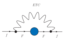
Figure 2: Ordinary fermion mass (f) in ETC models

As consequence, it is possible verify that the mass generated for the fermion (f) is given byholdom

$$m_{f}\approx C_{ETC}\alpha_{ETC}\frac{\mu^{3}_{{}_{TC}}}{M^{2}_{ETC}}\left(\frac{M_{ETC}}{\mu_{{}_{TC}}}\right)^{\gamma_{m}}.$$ (50)

In order to consider the contributions of radiative corrections for coupled system described in Fig.(1), without specifying a model, we will assume that $(Q^{\prime},Q,q)$ and TC are embedded into a ETC gauge group, where $Q=(U,D)$ , $Q^{\prime}=(U^{\prime},D^{\prime})$ and $q=(f,f^{\prime})$. The mass anomalous dimension $\gamma_{m}$ indicated in Eq.(50) should be replaced by $\gamma^{\prime}_{jm}$ with $F=(Q,Q^{\prime})$. In this case the calculation for $(m_{f})$ obtained from Fig. (2), leads to

$$m_{fj}\sim C_{ETC}\alpha_{ETC}\frac{\mu^{3}_{{}_{TC}}}{M^{2}_{ETC}}\left(\frac{M_{ETC}}{\mu_{{}_{TC}}}\right)^{\gamma_{m}+2\delta_{j}(\kappa_{j})}.$$ (51)

In addition to the corrections shown in Fig. 1, radiative ETC corrections to $\gamma_{m}$ lead to $\gamma_{m}+2\delta_{E}(\kappa_{E})$, with

$$\delta_{E}(\kappa_{E})=\frac{\kappa_{E}}{8+2\kappa_{E}}$$

and $\kappa_{E}\approx\alpha_{E}$. For a walking theory , where $\gamma_{m}\approx 1$, we can finally estimate that

$$m_{fj}\sim C_{ETC}\alpha_{ETC}\frac{\mu^{2}_{{}_{TC}}}{M_{ETC}}\left(\frac{M_{ETC}}{\mu_{{}_{TC}}}\right)^{2\delta_{j}(\kappa_{j})+2\delta_{E}(\kappa_{E})}=c\left(\frac{M_{ETC}}{\mu_{{}_{TC}}}\right)^{2\delta_{j}(\kappa_{j})+2\delta_{E}(\kappa_{E})-1}$$ (52)

where $c=C_{ETC}\alpha_{ETC}\mu_{{}_{TC}}$. Considering the Eqs.(23), (36) and (40), assuming $g^{2}_{X}\approx g^{2}_{{}_{TC}}$ and also the MAC hypothesis $C_{TC}\alpha_{TC}\sim 1$mac , with $\alpha_{E}\sim 0.032$us1 ; us2 , we get $2\delta_{1}(\kappa_{1})+2\delta_{E}(\kappa_{E})\sim O(0.65)$. A similar estimate considering Eqs.(23), (26), (36) and (40) can be made for $j=2$ leading to $2\delta_{2}(\kappa_{2})+2\delta_{E}(\kappa_{E})\sim O(0.3)$.

In the Ref.dne we consider a mechanism to generate mass split between different femionic generations, the first fermionic generation basically obtain mass due to the interaction with the QCD condensate, characterized by the effective scalar boson $\eta$. Whereas the third generation obtain mass due to its coupling with an TC condensate characterized by the effective scalar boson $\varphi$. The reason for this particular coupling is provided by the $SU(3)_{H}$ horizontal symmetry, where we assign different horizontal quantum numbers to first and third fermionic generations such that the couplings between these generations happen with the composite scalar bosons $\eta$ and $\varphi$.

The condensates formed by $Q$ and $Q’$ can be related to a system formed by two composite scalars denote by $\phi$ and $\phi’$. It is possible to consider a similar mechanism to that discussed in Ref.dne , where the introduction of a horizontal symmetry would provide only the coupling between the effective scalars $\phi$ and $\phi^{\prime}$ with fermions of the second (f) and third generation (f’) so that fermion couplings with exotic techniquarks $(U^{\prime},D^{\prime})$ are represented by $(f^{\prime})$, while with usual techniquarks by $(f)$.

In Fig. (3) we show the behavior of Eq.(52) for $SU(2)_{TC}$ , the curve (dotted-blue) correspond to $m_{f^{\prime}}$ , while the (dashed-orange) to $m_{f}$.

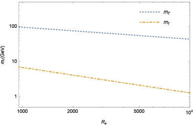
Figure 3: This figure shows the behavior of Eq.(52), where $m=m_{fj}$ and $R_{e}=\left(\frac{M_{ETC}}{\mu_{{}_{TC}}}\right)$. The curves depicted were obtained for technifermions in the fundamental representation of $SU(N_{TC})$[R=F].

VI Conclusions

In the Refs.us1 ; us2 we discussed a new approach consisting of models where TC and QCD are coupled through a larger theory, in this case the solutions of these equations are modified compared to those of the isolated equations , which allows us to build models where ETC boson masses can be pushed to very high energies. We calculated numerically the self-energy ($\Sigma(p^{2})$) of two coupled strong interaction theories and verified that the coupled TC self-energy behaves as Eq.(1).

In this work we extend the results obtained inus1 ; us2 for 331-TC models , considering the coupled system described in Fig.(1) we find that $(U^{\prime},U)$ self-energies have a much smoother dependence with the momentum than $1/p$ (walk). The diagrams on the right-hand side of Fig.(1), $(a_{4})$ and $(b_{4})$, plays the same role of the ETC interactions in the coupled system discussed in us1 ; us2 . The $V^{\pm},U^{\pm\pm}$ interactions modify the UV boundary condition of the SDE in differential form exactly as happens in (QCD and $SU(2)_{{}_{TC}}$) case in such a way that the ultraviolet behavior of the $(U^{\prime},U)$self-energies turn out to be of the form of Eq.(1), being this result confirmed by the behavior presented in Eq.(52).

The condensates formed by $Q$ and $Q’$ can be related to a system formed by composite scalars $\phi(\phi’)$, in the section 5 considering an extension of the mechanism proposed in Ref.dne , we discussed the possibility of generating the mass splitting between the second and third generation of fermions. The Fig.(3) illustrates how the mass splitting of the order $O(100)GeV$(dashed-dotted lines) could be generated for $\frac{M_{ETC}}{\mu_{{}_{TC}}}=10^{3}$ or $M_{ETC}=O(10^{6})GeV$ for $c\sim O(1)TeV$.

The composite scalars bosons $\phi(\phi^{\prime})$ mimics the behavior of a (2HDM) that can lead to interesting phenomenological implications. The few aspects discussed here show that models along the line of coupled strong interactions may open way for the construction of realistic theories of dynamical symmetry breaking.

VII References

References

• (1) Y. Nambu and G. Jona-Lasinio, Phys. Rev. 122, 345 (1961).
• (2) S. Weinberg, Phys. Rev. D 13, 974 (1976); S. Weinberg, Phys. Rev. D 19 1277 (1979).
• (3) L. Susskind, Phys. Rev. D 20, 2619 (1979); S. Dimopoulos and L. Susskind, Nucl. Phys. B155 , 237 (1979).
• (4) C. T. Hill and E. H. Simmons, Phys. Rept. 381, 235 (2003) [Erratum-ibid. 390, 553 (2004)].
• (5) F. Sannino, hep-ph/0911.0931, Lectures presented at the 49th Cracow School of Theoretical Physics. Conformal Dynamics for TeV Physics and Cosmology, Cracow, Nov , 2009; Acta Phys. Polon.. B 40, 3533 (2009); Int. J. Mod. Phys. A 20, 6133 (2005).
• (6) K. Lane, Technicolor 2000 , Lectures at the LNF Spring School in Nuclear, Subnuclear and Astroparticle Physics, Frascati (Rome), Italy, May 15-20, 2000.
• (7) Holdom B., Phys. Rev. D 24, 1441 (1981).
• (8) K. D. Lane and M. V. Ramana, Phys. Rev. D 44, 2678 (1991).
• (9) T. W. Appelquist, J. Terning and L. C. R. Wijewardhana, Phys. Rev. Lett. 79, 2767 (1997).
• (10) K. Yamawaki, Prog. Theor. Phys. Suppl. 180, 1 (2010); and hep-ph/9603293.
• (11) Y. Aoki et al., Phys. Rev. D 85, 074502 (2012).
• (12) T. Appelquist, K. Lane and U. Mahanta, Phys. Rev. Lett. 61, 1553 (1988).
• (13) T. Appelquist, M. Piai, and R. Shrock, Phys. Rev. D69, 015002 (2004).
• (14) T. Appelquist, M. Piai and R. Shrock, Phys. Lett. B 593 , 175 (2004).
• (15) T. Appelquist and R. Shrock, Phys. Rev. Lett. 90, 201801-1 (2003).
• (16) T. Appelquist and R. Shrock, Phys. Lett. B 548 , 204 (2002).
• (17) M. Kurachi, R. Shrock and K. Yamawaki, Phys. Rev. D 76, 035003 (2007).
• (18) V. A. Miransky and K. Yamawaki, Mod. Phys. Lett. A 4, 129 (1989).
• (19) K.-I. Kondo, H. Mino and K. Yamawaki, Phys. Rev. D39, 2430 (1989).
• (20) V. A. Miransky, T. Nonoyama and K. Yamawaki, Mod. Phys. Lett. A4, 1409 (1989).
• (21) T. Nonoyama, T. B. Suzuki and K. Yamawaki, Prog. Theor. Phys.81, 1238 (1989).
• (22) V. A. Miransky, M. Tanabashi and K. Yamawaki, Phys. Lett. B221, 177 (1989).
• (23) K.-I. Kondo, M. Tanabashi and K. Yamawaki, Mod. Phys. Lett. A8, 2859 (1993).
• (24) T. Takeuchi, Phys. Rev. D 40, 2697 (1989).
• (25) A. Doff, Eur.Phys.J. C 76, 33 (2016).
• (26) A. Doff, Int. J. Mod. Phys. A 34, 1950030 (2019).
• (27) A. Doff, Phys.Rev. D 76, 037701 (2007).
• (28) A. Doff, Phys.Rev. D 81, 117702 (2010).
• (29) A. Doff and A. A. Natale, Phys.Rev. D 87, 095004 (2013).
• (30) A. C. Aguilar, A. Doff and A. A. Natale, Phys. Rev. D 97, 115035 (2018).
• (31) A. Doff and A. A. Natale, Eur. Phys. J. C 78, 872 (2018).
• (32) M. Singer, J. W. F. Valle and J. Schechter, Phys. Rev. D 22, 738 (1980).
• (33) F. Pisano and V. Pleitez, Phys. Rev. D 46, 410 (1992).
• (34) P. H. Frampton, Phys. Rev. Lett. 69, 2889 (1992).
• (35) R. Foot, H. N. Long and Tuan A. Tran, Phys. Rev. D 50, 34 (1994).
• (36) V. Pleitez and M.D. Tonasse, Phys. Rev. D48, 2353 (1993).
• (37) F. Pisano, Mod. Phys. Lett A 11, 2639 (1996).
• (38) A. Doff and F. Pisano, Mod. Phys. Lett A 14, 1133 (1999).
• (39) A. Doff and F. Pisano, Phys.Rev. D 63, 097903 (2001)
• (40) C. A. de S. Pires and O. P. Ravinez, Phys. Rev. D 58, 035008 (1998).
• (41) C. A. de S. Pires, Phys. Rev. D 60, 075013 (1999).
• (42) P. V. Dong and H. N. Long, Int. J. Mod. Phys. A 21, 6677 (2006).
• (43) Prasanta Das and Pankaj Jain, Phys. Rev. D 62, 075001 (2000).
• (44) Craig D. Robertz and Bruce H. J. McKellar, Phys. Rev.D 41, 672 (1990).
• (45) J. M. Cornwall, Phys. Rev. D 26, 1453 (1982).
• (46) A. C. Aguilar, D. Binosi and J. Papavassiliou, Phys. Rev. D 78, 025010 (2008).
• (47) A. C. Aguilar and J. Papavassiliou, Phys. Rev. D 83, 014013 (2011).
• (48) A. Doff, F. A. Machado and A. A. Natale, Annals of Physics 327, 1030 (2012).
• (49) A. Cohen and H. Georgi, Nucl. Phys. B 314, 7 (1989).
• (50) Richard W. Haymaker and Juan Perez-Mercader, Phys. Rev. D 27, 1353 (1983).
• (51) K. Lane, Phys. Rev. D 10, 2605 (1974).
• (52) S. Raby, S. Dimopoulos, and L. Susskind, Nucl. Phys. B 169, 373 (1980).
• (53) A. Doff and A. A. Natale, Eur. Phys. J. C 32, 417 (2003).