SKEWED PROBIT REGRESSION - IDENTIFIABILITY, CONTRACTION AND REFORMULATION

Abstract

Skewed probit regression is but one example of a statistical model that generalizes a simpler model, like probit regression. All skew-symmetric distributions and link functions arise from symmetric distributions by incorporating a skewness parameter through some skewing mechanism. In this work we address some fundamental issues in skewed probit regression, and more genreally skew-symmetric distributions or skew-symmetric link functions.

We address the issue of identifiability of the skewed probit model parameters by reformulating the intercept from first principles. A new standardization of the skew link function is given to provide and anchored interpretation of the inference. Possible skewness parameters are investigated and the penalizing complexity priors of these are derived. This prior is invariant under reparameterization of the skewness parameter and quantifies the contraction of the skewed probit model to the probit model.

The proposed results are available in the R-INLA package and we illustrate the use and effects of this work using simulated data, and well-known datasets using the link as well as the likelihood.

1 INTRODUCTION

Skew-symmetric distributions have acclaimed fame due to their ability to model skewed data, by introducing a skewness parameter to a symmetric distribution, through some skewing mechanism. In the preceding decades, an abundance of skewed distributions has been proposed from the basis of symmetric distributions, like the skew-normal [27, 3], skew-t [6] and more generally skew-elliptical distributions [20]. In each of these skew distributions, an additional parameter is introduced that indicates the direction of skewness or alternatively, symmetry.

With the introduction of the additional parameter, the inferential problem can become more challenging. The identifiability of the parameters and the existence of the maximum likelihood estimators (MLEs) are issues to keep in mind. In the Bayesian paradigm, the choice of a prior for the skewness parameter emerges. Either way, the inference of the skewness parameter is crucial in evaluating the appropriateness of the underlying (skewed) model.

A continuous random variable $X$, follows a skew-normal (SN) distribution with location, scale and skewness(shape) parameters $\xi,\omega$ and $\alpha$, respectively, if the probability density function (pdf) is as follows:

$$g(x)=\frac{2}{\omega}\phi\left(\frac{x-\xi}{\omega}\right)\Phi\left[\alpha\left(\frac{x-\xi}{\omega}\right)\right],$$ (1)

where $\alpha\in\Re$, $\omega>0$, $\xi\in\Re$, and $\phi(\cdot)$ and $\Phi(\cdot)$ are the density and cumulative distribution function (CDF) of the standard Gaussian distribution, respectively. Denote by $G(x)$ the CDF of the skew-normal density.

The parameterisation in (1) poses difficulties since the mean and variance depends on $\alpha$, as $E[X]=\xi+\omega\delta\sqrt{2/\pi}$ and $V[X]=\omega^{2}\left(1-2\delta^{2}/\pi\right)$, where $\delta=\alpha/\sqrt{1+\alpha^{2}}$. This implies that inference for $\alpha$ will also influence the inference for the mean and variance, since both are functions of $\alpha$.

A similar challenge arises in the binary regression framework where the skew-normal link function is used as a generalization of probit regression, namely skewed probit regression. The need for asymmetric link functions have been noted by [14]. In binary regression, asymmetric link functions are essential in cases where the probability of a particular binary response approaches zero and one at different rates. In this case, a symmetric link function will result in substantially biased estimators with over(under)estimation of the mean probability of the binary response, due to the different rates of approaching zero and one (see [16] for more details on this issue). Skewed probit regression is an extension of probit regression, where covariates are transformed through the skew-normal CDF instead of the standard normal CDF.

Here, it might not be intuitive when the skewed link function is more appropriate than the symmetric link function. The estimate of the skewness parameter could provide some insights into this, only if the inference of the skewness parameter is reliable and interpretable.

Regarding the inference of the skewness parameter, $\alpha$ in (1), being it in the skewed probit regression or the skew-normal distribution as the underlying response model (which are conceptually the same estimation setup), various works have been contributed, most of them dedicated to the skew-normal response model framework. The identifiability of the parameters in the skew-normal response model was investigated by [21] (and skew-elliptical in general), [28] (for finite mixtures) and [13] (for extensions of the skew-normal distributions). For binary regression, identifiability of the parameters was considered by [23] where some issues concerning identifiability were raised. We address the identifiability problem from a first principles viewpoint, so that the parameters are identifiable, even with weak covariates, hence adding to [23].

In the skew-normal response model, the bias of the MLEs is a well-known fact (see [30] for more details). For small and moderate sample sizes, the MLE of the skewness parameter could be infinite with positive probability and the profile likelihood function has a singularity as the skewness parameter approaches zero, as noted early on by [3] (see also [24]). Some approaches to alleviate this feature of the skew-normal likelihood function have been proposed, including reparameterization of the model by [3] using the mean and variance (instead of location and scale parameters), or using a Bayesian framework by [25] (default priors) and [7] (proper priors). Also, [30] used the work of [19] to propose an adjusted (penalized) score function for frequentist estimation of the skewness parameter. A penalized MLE approach for all the parameters, including the skewness parameter, is presented by [5]. Bias-reduction regimes were proposed by [26].

From a Bayesian viewpoint, various priors for the skewness parameter have been proposed such as the Jeffrey’s prior [25], truncated Gaussian prior [1], Student t prior and approximate Jeffery’s prior [7], uniform prior [2], probability matching prior [11], informative Gaussian and unified skew-normal priors [12] and the beta-total variation prior [17]. All of these Bayesian approaches, with the exception of the latter, are based on somewhat arbitrary prior choices for mainly mathematical or computational convenience. These priors (as many others) are not invariant under reparameterization of the skewness parameter. The beta-total variation prior presented by [17] is based on the total variation from the symmetric Gaussian model to the skew-normal model, viewing the skewness parameter as a measure of perturbation. This prior is indeed invariant under one-to-one transformation of the skewness parameter.

Amongst the many works on the skew-normal response model, it seems that the genesis of the skew-normal model has been neglected. The skew-normal model was introduced by [3] as an (asymmetric) extension of the Gaussian model. The motivation for this extension is found in data. When data behaves like the Gaussian model, but the profile of the density is asymmetric, the skew-normal model might be appropriate. Conversely, we need an inferential framework wherein the skew-normal model would contract (or reduce) to the Gaussian model, in the absence of sufficient evidence of non-trivial skewness. The priors mentioned before do not provide a quantification framework with which the modeler can understand, and subsequently control this contraction. To achieve this, we need to consider the model (either skewed probit regression or the skew-normal response model) from an information theoretic perspective. Then we can construct a prior with which the quantification of contraction (or not) can be done, and used as a translation of prior information from the modeler to the model.

In this paper we address some issues (identifiability, standardizing, skewness parameters) prevalent in skewed-probit regression in Section 2 and construct the penalized complexity (PC) prior for the skewness parameter of the link function (which is translatable to the skew-normal response model) in Section 4. This PC prior is implemented in the R-INLA [29] package for general use by others. We use a numerical study to illustrate the solutions proposed in Section 2 and apply the PC prior to simulated and real data in Sections 5 and Section 6. The paper is concluded by a discussion in Section 7 in which we sketch the wider applicability of this work and contributions to the wider skew-symmetric family.

2 SKEWED PROBIT REGRESSION AND ISSUES

We consider skewed probit regression as an extension of probit regression, where the link function is the skew-normal CDF instead of the standard normal CDF. We formulate skewed probit regression that can include random effects like spline functions of the covariates, spatial and/or temporal effects. For this paper, we assume the following structure. From a sample of size $n$, the responses $\boldsymbol{y}_{n\times 1}$ are counts of successful trials out of $N_{n\times 1}$ trials and hence we assume a Binomial distribution with success probability $p$. We gather all $m$ covariates in $\boldsymbol{X}_{n\times m}$ and use these to build an additive linear predictor, defined as $\boldsymbol{\eta}_{n\times 1}$. So then,

$$y_{i} \sim \text{Binomial}(N_{i},p_{i})$$

$$p_{i} = G(\eta_{i}),\quad i=1,\ldots,n$$ (2)

where $G(\cdot)$ is the CDF of the Skew-Normal that depends on $(\xi,\omega,\alpha)$. The linear predictor $\eta_{i}$ is an additive linear predictor defined as follows,

$$\eta_{i}=\beta_{0}+\boldsymbol{\beta}^{\prime}\boldsymbol{X}_{i}+\sum_{k=1}^{K}f^{k}(\boldsymbol{Z}_{i}),$$ (3)

where $\boldsymbol{X}$ and $\boldsymbol{Z}$ are the covariates for the fixed and random effects, respectively, the functions $\{f^{k}(.)\}$ are random effects like spatial, spline, temporal effects with hyperparameters $\boldsymbol{\theta}$.

2.1 Issue 1 - Standardizing the link function

With the aim of standardizing the link function, [23] assumed $\xi=0,\omega=1$, similar to [9] and many others. Initially, the idea behind this choice feels intuitive since the skew probit link is an extension of the probit link through the skewness parameter. However, the $(0,1)$ parameter values of the probit link should not be naively copied to the skewed probit link. The choice, $\xi=0,\omega=1$ implicitly concedes that a skew-normal density (1) with mean

$$E[X]=\alpha\sqrt{\frac{2}{\pi(1+\alpha^{2})}},$$

and variance

$$V[X]=1-\frac{2\alpha^{2}}{\pi(1+\alpha^{2})},$$

is used to calculate the probability of success, for all $\alpha$. This essentially implies that for different skewness parameter values, different means and variances are used. This way of standardizing is a parameter-based method, instead of the intended property-based method like in the probit link. We do not expect the assumption $\xi=0,\omega=1$ to work well since the mean and variance are not anchored and can attain many values based on different values of $\alpha$.

We posit that the mean and the variance (properties of the link) should be fixed, like in the probit case, instead of the skew-normal location and scale parameters. This is analogous to the idea of the centered parametrization of the skew-normal density and mentioned by [8].

We propose the link function $F(y|\alpha)$ that is the CDF of the Skew-Normal density (1) scaled to have zero mean and unit variance for all values of $\alpha$. That is,

$$F(y|\alpha)=\int_{-\infty}^{y}f(x|\alpha)\,dx$$

where

$$f(x|\alpha)=\frac{2}{\omega(\alpha)}\phi\left(\frac{x-\xi(\alpha)}{\omega(\alpha)}\right)\Phi\left[\alpha\left(\frac{x-\xi(\alpha)}{\omega(\alpha)}\right)\right],$$ (4)

$$\xi(\alpha)=-\omega\alpha\sqrt{\frac{2}{\pi(1+\alpha^{2})}},$$

and

$$\omega(\alpha)=\sqrt{\left(1-\frac{2\alpha^{2}}{\pi(1+\alpha^{2})}\right)^{-1}}.$$

This provides an anchored link function with zero mean and unit variance, for all $\alpha$. If this standardization is not used then an arbitrary unknown scale is introduced to the model, with no means of recovering it. By fixing the mean and variance, we have a better understanding of the properties of the link and we do approach the probit case in the neighborhood of $\alpha=0$.

2.2 Issue 2 - The quantile intercept and identifiability of parameters

The identifiability of the parameters in skewed probit regression were first investigated by [23]. They showed that without the presence of a continuous covariate, the intercept $\beta_{0}$, and skewness parameters are not identifiable. This is expected due to the traditional definition of the skewed probit model (2) and (3). We rectify the formulation of the skewed probit regression intercept, by introducing the quantile intercept, and subsequently solve this issue of non-identifiability by returning to first principles.

In simple linear regression, the intercept is used to calculate the expected value of the linear predictor without any effect from covariates. In probit regression, the intercept contains information about the probability of the event, without the effects from covariates. The value of the intercept should not provide any information about the other parameters in the model.

However, when we introduce a skewness parameter to a symmetric family to formulate a skew-symmetric link then we are fundamentally changing the meaning of what is traditionally called the intercept of the linear predictor, i.e. $\beta_{0}$ in (3).

Consider probit regression with one centered covariate $X$,

$$p=\text{Prob}[Y=1]=\Phi(\beta_{0}+\beta_{1}X).$$

Now if $\beta_{1}X=0$, then

$$q=\text{Prob}[Y=1]=\Phi(\beta_{0}),$$

which implies that $\beta_{0}$ is the $q^{\text{th}}$ quantile of the standard Gaussian distribution. There is thus a one-to-one relationship between $q$ and $\beta_{0}$. When $\beta_{1}\neq 0$, then $\text{Prob}[Y=1]$ changes because of $\beta_{1}X$, without affecting $\beta_{0}$, because $\Phi$ remains the same function. In this sense, $\beta_{0}$ is uninformative for $\beta_{1}$.

Conversely, consider skewed-probit regression from (2) and (4),

$$p=\text{Prob}[Y=1]=F(\beta_{0}+\beta_{1}X|\alpha).$$

Here, $\beta_{0}$ should, in the same way, be uninformative for $\beta_{1}$. This does not hold because the dependence of $\alpha$. We can ensure this, if

$$q=\text{Prob}[Y=1]=F(\beta_{0}|\alpha)$$

is constant for varying $\alpha$, which is the case if $\beta_{0}$ is defined as the $q^{\text{th}}$ quantile of the distribution with CDF $F$. Therefore, we reformulate $\beta_{0}$ as

$$\beta_{0}(q,\alpha)=F^{-1}(q|\alpha),$$ (5)

so $\beta_{0}$ is the $q^{\text{th}}$ quantile of $F(.|\alpha)$. The quantile level $q$ is now the unknown intercept-parameter instead of $\beta_{0}$.

Note that there is (generally) not a one-to-one relationship between $\beta_{0}$ and $q$ since the $q^{\text{th}}$ quantile depends on $\alpha$. In this new formulation, the intercept as defined implicitly by $q$, provides no information about $\beta_{1}$ and parameters of $F(\eta_{i}|\alpha)$ are identifiable. We return in 5.3 to a numerical study of this issue.

This formulation might seem surprising at first sight, but in the case of a symmetric link, the intercept is the quantile of a distribution with fixed (no) skewness. In the case of the probit or identity links for example, this formulation will reduce to the usual intercept parameter since in these cases there is a one-to-one relationship between $\beta_{0}$ and $q$.

In terms of implementation in R-INLA, the new formulation of the skew normal model in terms of $q$ is available and subsequently, the prior distribution for $q$ can be derived from a corresponding informative $N(\mu_{0},\tau_{0})$ prior for $\beta_{0}$ in the case where $\alpha=0$. This will ensure that the probit and the skewed-probit models have comparable priors for their respective ”intercept” parameters.

2.3 Issue 3 - Skewness-related parameters

It is well-known that the skew-normal likelihood has a (double) singularity in the neighbourhood $\alpha\simeq 0$ [3]. Various adaptations of maximum likelihood estimation and some Bayes estimators have been proposed as solutions to this singularity. [22] used the Fisher information to propose a reparameterization that uses $\alpha^{3}$ as the skewness parameter since this solves the double singularity problem in the likelihood. In our venture to derive the PC prior for the skewness, we derived the Kullback-Leibler divergence (KLD) from the skew-normal link to the probit link and noticed the same feature as mentioned in [22]. This resemblance is expected since the Fisher information metric is the Hessian of the KLD.

From (4), the KLD for small $|\alpha|$ can be found to be

$$\text{KLD}(\alpha) = \int f(x|\alpha)\log\frac{f(x|\alpha)}{f(x|\alpha=0)}dx$$ (6)

$$= \frac{\pi^{2}+16-8\pi}{6\pi^{3}}\alpha^{6}-\frac{144\pi+3\pi^{3}-38\pi^{2}-168}{6\pi^{4}}\alpha^{8}$$

$$+\frac{-42240\pi-2560\pi^{3}+16176\pi^{2}+129\pi^{4}+39936}{120\pi^{5}}\alpha^{10}+\mathcal{O}(\alpha^{12})$$

$$\approx c_{1}\alpha^{6}+c_{2}\alpha^{8}+c_{3}\alpha^{10}.$$

Interestingly, the behavior of $\alpha$ around $\alpha=0$ does not have the usual asymptotics (consistency rate of $\sqrt{n}$) since the leading term is $\alpha^{6}$. This implies that the estimator of $\alpha$ in the neighbourhood $\alpha\simeq 0$, has a consistency rate $n^{\frac{1}{6}}$ but a skewness parameter $\gamma=\alpha^{3}$, such that $\alpha=\text{sign}(\gamma)\sqrt[3]{|\gamma|}$, will have the normal asymptotics in the sense that the estimator of $\gamma$ will be $\sqrt{n}$ consistent.

Even though $\gamma$ has the usual asymptotic behaviour, the estimate of it is hard to interperate since it does not relate easily to an interpretable property. We can instead focus on the more intepretable (standarised) skewness of the skew-normal distribution, $\gamma_{1}$, which is a monotone function of $\gamma$

$$\gamma_{1}=\frac{(4-\pi)\left(\sqrt{\frac{2\delta^{2}}{\pi}}\right)^{3}}{2(1-\frac{2\delta^{2}}{\pi})^{\frac{3}{2}}},$$ (7)

where $\delta=\frac{\alpha}{\sqrt{1+\alpha^{2}}}$ (and $\gamma=\alpha^{3}$). The skewness take values in the interval $-0.99527<\gamma_{1}<0.99527$, which is correct up to five digits.

The question arises if we should formulate a prior for $\alpha$, $\gamma$ or the skewness $\gamma_{1}$. If priors are assigned more ad-hoc parameters, this question poses a challenge. The PC prior is invariant under reparameterizations [31], implying that this framework will produce equivalent priors for $\alpha$, $\gamma$ and $\gamma_{1}$. They are equivalent in the inferential sense, and will produce the same posterior inference.

3 SKEW-NORMAL MEAN REGRESSION

In this section we focus on skew-normal regression, although these issues also exist in more general skew-symmetric regression models.

In the preceeding section we mentioned the different parameters that can be used to capture the skewness in the skewed probit model, and the proposals pertain to the skew-normal regression model as well.

Most works on skew-normal regression propose a regression model for the location parameter, $\xi$, from (1). This generalization of Gaussian regression seems straightforward but when we keep in mind that the location parameter of the Gaussian is equal to the mean, then we can see that regressing through the location parameter of the skew-normal is not practical. In the spirit of generalizing Gaussian regression to skew-normal regression, we should formulate the regression model based on the mean. Hence for $y_{i}\sim SN(\xi,\omega,\alpha)$ from (1),

$$E[Y_{i}]=\eta_{i},$$ (8)

with $\eta_{i}$ from (3), instead of $\xi_{i}=\eta_{i}$. Note that here we do not reformulate the intercept as in Section 2.2 for skewed probit regression, since the identity link function is used. We illustrate the proposed skew-normal regression model in Section 6.

4 PENALIZING COMPLEXITY PRIOR FOR THE SKEWNESS PARAMETER

The work of [31] introduced the notion of penalizing complexity priors for parameters and provided the framework for deriving priors that quantify the contraction from a complex model to a simpler model. These PC priors are especially helpful and very needed in cases where priors have traditionally been chosen due to mathematical convenience, or convention.

In this section we derive the PC prior for $\alpha$ due to the invariance of the PC prior under reparameterization of the skewness parameter. The derivations of the PC prior for $\gamma$ and $\gamma_{1}$ follows then directly from a change-of-variable exercise.

Using [31] and (6), define the uni-directional distance from the skew-normal to the Gaussian density as,

$$d(\alpha) = \sqrt{2\text{KLD}(\alpha)}$$ (9)

$$\approx \sqrt{2(c_{1}\alpha^{6}+c_{2}\alpha^{8}+c_{3}\alpha^{10})}$$

The penalizing complexity prior for the skewness parameter $\alpha$ is then formed by assigning an exponential prior with parameter $\theta$ to the distance. The parameter $\theta$ incorporates information from the user to control the tail behavior and thus the rate of contraction towards the probit link function. The penalizing complexity prior follows then directly, as

$$\pi(\alpha) = \frac{1}{2}\theta\exp\left[-\theta d(\alpha)\right]\left|\frac{\partial d(\alpha)}{\partial\alpha}\right|$$ (10)

$$\approx \frac{\theta}{2\sqrt{2(c_{1}\alpha^{6}+c_{2}\alpha^{8}+c_{3}\alpha^{10})}}\left|2(6c_{1}\alpha^{5}+8c_{2}\alpha^{7}+10c_{3}\alpha^{9})\right|$$

$$\times\exp\left[-\theta|\alpha^{3}|\sqrt{2(c_{1}+c_{2}\alpha^{2}+c_{3}\alpha^{4})}\right].$$

for small values of $|\alpha|$. The user-defined parameter $\theta$ is used to govern the contraction towards probit regression, e.g., for small $p_{U}>0$,

$$\text{Prob}(d(\alpha)>U) = p_{U}=\exp(-\theta U)$$

which gives $\theta=-{\log p_{U}}/{U}$. There is no explicit expression for the penalizing complexity prior of $\alpha$ in general, but the prior can be computed numerically. The prior for $\gamma_{1}$ is available in the R-INLA package[29] with prior = "pc.sn" and parameter param=$\theta$. We use the $\gamma_{1}$ reparameterization, since $\gamma_{1}$ quantifies the skewness as a property with good interpretation.

The PC priors of $\alpha$ and $\gamma_{1}$ are illustrated in Figure 1 for $\theta=5$, on the $\alpha$ and $\gamma_{1}$ scales. In Figure 2 various values for $\theta$ are considered to provide an intuition about the effect of $\theta$.

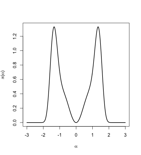
Figure 1: PC prior (10) for $\theta=5$ on the $\alpha$ scale (left) and the $\gamma_{1}$ scale (right)

From Figure 1 we can see the shape of the PC prior for $\alpha$ is quite peculiar, but has a clear interpretation in terms of a prior on the distance. It just shows that if we assign priors to parameters, like $\alpha$, instead of to a property, like $\gamma_{1}$, it is highly improbable that we could think of a density function for the parameter that has good translatable properties. Another interesting note is that from the prior density of $\alpha$ around $\alpha=0$, we can see that most priors of $\alpha$ proposed in literature actually results in underfitting, instead of the usual overfitting, since they assign too much density to the neighborhood around $\alpha=0$. Conversely, the PC prior of $\gamma_{1}$ is as expected with a mode at the value for the probit link.

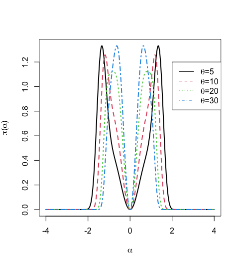
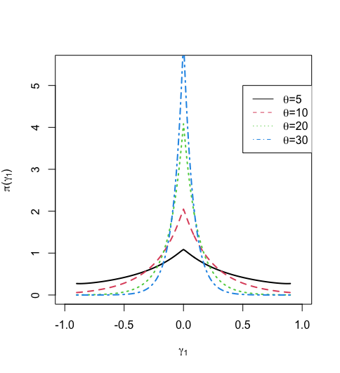
Figure 2: PC prior (10) for various $\theta$’s on the $\alpha$ scale (left) and the $\gamma_{1}$ scale (right)

5 SIMULATION STUDY

In this section we present condensed results from a simulation study with the aim to show the results proposed in this work for experiments with a large and small number of trials. The setup is to simulate linear predictors $\eta_{i}=\beta_{0}(\alpha,q)+\beta_{1}x_{i}$, where $x_{i}\sim\text{N}(0,0.5)$ for $i=1,\ldots,n$. The success probabilities are then $p_{i}=F(\eta_{i}|\alpha)$ from (2) and subsequently the response variable $y_{i}$, wherere $y_{i}\sim\text{Bin}(N_{i},p_{i})$. Throughout, we assume $\theta=5$ for the PC prior and a weak Gaussian prior with parameters $(0,10^{2})$ for the skewness.

5.1 Large number of trials

For an experiment that consists of a large number of trials, we consider four simulation scenario’s which can be summarized as:

1. $q=\frac{1}{3},\beta_{1}=1,\gamma_{1}=0(\alpha=0),N_{i}=200$

2. $q=0.25,\beta_{1}=-1,\gamma_{1}=\frac{2}{3}(\alpha=10),N_{i}=200$

3. $q=0.30,\beta_{1}=1,\gamma_{1}=\frac{1}{3}(\alpha=2),N_{i}=200$

4. $q=0.10,\beta_{1}=-1,\gamma_{1}=-\frac{1}{3}(\alpha=-2),N_{i}=200$

In each case we consider the PC prior as well as the Gaussian prior for the skewness $\gamma_{1}$, and weakly informative Gaussian priors for the fixed effects.

5.1.1 Results

The fixed effects were recovered well and here we focus on the skewness $\gamma_{1}$. From Table 1 it is clear that the PC prior (and the Gaussian prior) performs as expected since the sample size and number of trials are large. In Figure 3 the posterior results for the skewness are summarised with coverage probability and median length of the credible interval. The results for other scenarios are similar and omitted here. From this (and many other) simulation studies, we conclude that for a large number of trials the skewed-probit link works well and the inference is accurate. It is clear that the PC prior does not contract towards the probit model when the data presents strong support for the skewed probit model (scenarios 2,3 and 4).

Scenario	PC prior		Gaussian prior
	CP	MLCI	CP	MLCI
1	$95$	$0.28$	$94$	$0.35$
2	$96$	$0.28$	$97$	$0.34$
3	$95$	$0.31$	$95$	$0.34$
4	$95$	$0.32$	$95$	$0.35$

Table 1: Coverage probability (CP) and median length of the credible interval (MLCI) for the skewness $\gamma_{1}$ under the PC and Gaussian (G) priors, for large $N_{i}$

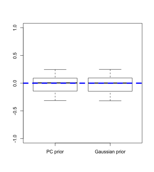
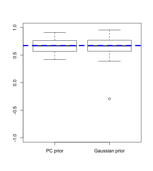
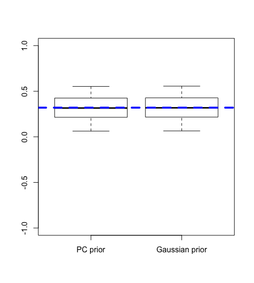
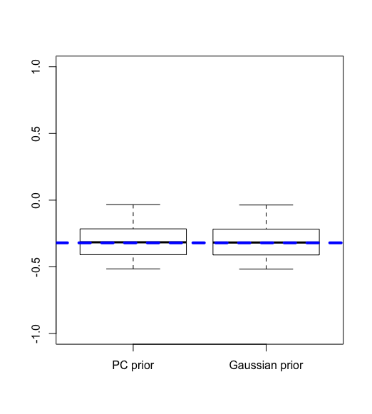
Figure 3: Median of $95\%$ credible intervals for the different scenario’s with the true skewness (dashed line): Scenario 1, 2, 3 and 4 from left to right

5.2 Small number of trials

Here we focus our attention on samples of size $200$ of binary trials, and the scenario’s we consider are:

1. $q=\frac{1}{2},\beta_{1}=1,\gamma_{1}=-\frac{2}{3}(\alpha=-10),N_{i}=1$

2. $q=\frac{1}{2},\beta_{1}=1,\gamma_{1}=0(\alpha=0),N_{i}=1$

We consider the PC prior as well as the Gaussian prior for the skewness parameter, and weakly informative Gaussian priors for the fixed effects.

5.2.1 Results

From Table 2 it is clear that the skewness is not recovered well for a small number of trials. In the case of the PC prior, the coverage is poor but the credible intervals are still relatively narrow. For the Gaussian prior, the coverage is high mainly due to the very wide credible intervals. For a small number of trials or binary trials, the skewness is hard to capture. Even though the nominal coverage for the Gaussian prior is still high from Table 2, the median length of the credible interval implies that the credible intervals span most of the support of $\gamma_{1}$. However, the PC prior contracts to zero with relatively narrow credible intervals and exhibits poor coverage for $\gamma_{1}\neq 0$. It is evident that the skewness is hard to estimate with a small number of trials. This is not unexpected since in binary data, we only observe a success or failure for each subject and subsequently the data does not provide sufficient information about the skewness. We need repetitions in the data to learn more about the skewness. We can see in Figure 4 that the PC prior contracts to zero if there is not enough evidence for the skewed link, but the Gaussian prior proposes an arbitrary value for the skewness from most of the range of $\gamma_{1}$ (possibly with the wrong sign as in Figure 4]). In this case, using the skewed-probit link for binary data might not be useful.

Scenario	PC prior		Gaussian prior
	CP	MLCI	CP	MLCI
1	$65$	$0.41$	$90$	$1.24$
2	$95$	$0.33$	$90$	$1.45$

Table 2: Coverage probability (CP) and median length of the credible interval (MLCI) for the skewness $\gamma_{1}$ under the PC and Gaussian (G) priors, for small $N_{i}$

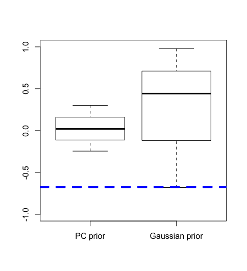
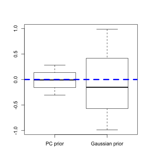
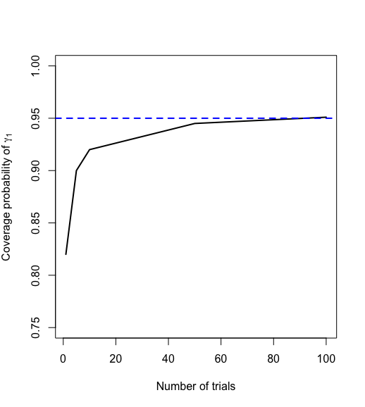
Figure 4: $95\%$ credible intervals for $\gamma_{1}$ with $n_{i}=1$ and $\gamma_{1}=-\frac{2}{3}$ (left) or $\gamma_{1}=0$ (middle). Coverage probabilities for $\gamma_{1}$ under scenario 1 as $n_{i}$ increases (right)

5.3 Confounding and the effect of the quantile intercept

In this section we look at the effect of not using the new quantile intercept. We used a simulated dataset, similar to the preceeding section, with $q=0.4,\beta_{1}=0.1,\gamma_{1}=-\frac{2}{3}$. In this setup the linear predictor is close to zero, for a centered covariate, the confounding between the classical intercept and the skewness parameter is clear. In Figure 5 the median of the $95\%$ credible intervals of the skewness (for 500 repetitions) as well as the true value of the skewness are presented. On the left we have the case of the quantile intercept and on the right, the classical intercept. By using the classical intercept, as in the case of GLM, the skewness is not estimated correctly in the sense that the direction is not even recovered. It is clear that the quantile intercept solves the confounding of the intercept of the linear predictor, with the skewness of the link.

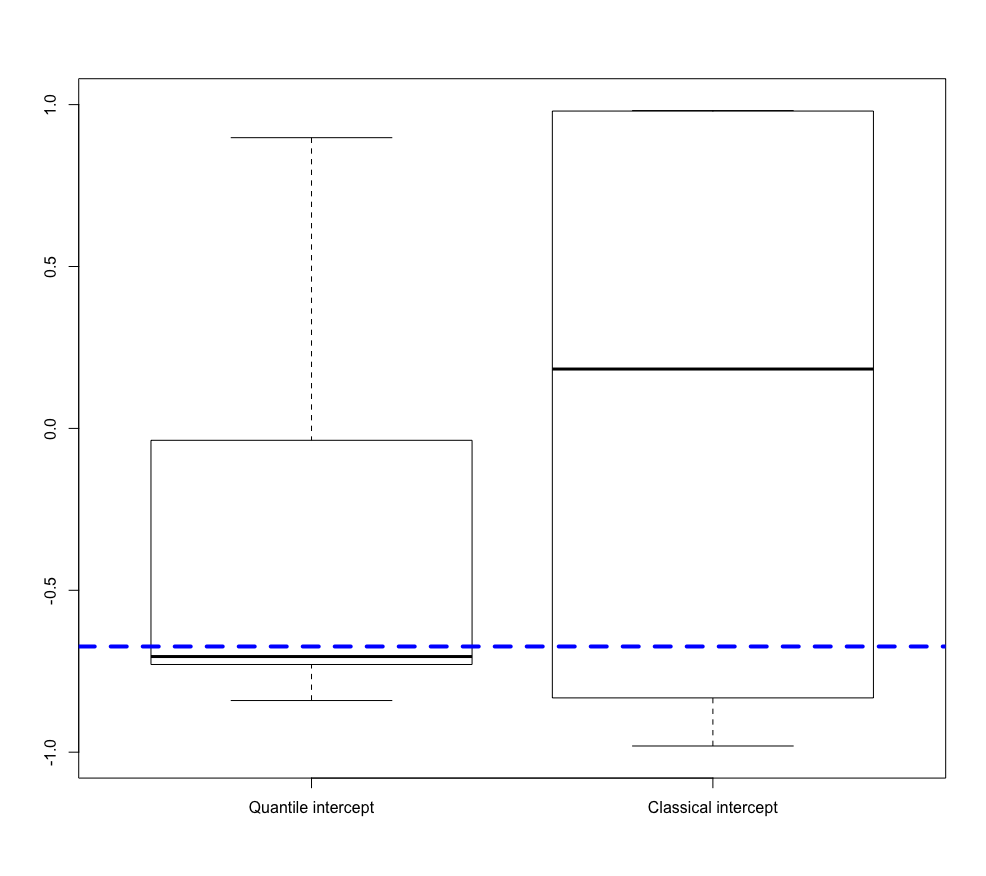
Figure 5: Median credible intervals for the skewness $\gamma_{1}$ using the quantile intercept vs the classical intercept

6 APPLICATIONS

In this section we illustrate the use of skewed probit regression with the PC prior using two well-known datasets, the beetle mortality data [10] (binomial response with multiple trails) and the UCI Cleveland heart disease data [18] (Bernoulli response). We also present the analysis of the Wines data to illustrate the use of this work in the skew-normal likelihood.

6.1 Beetle mortality data

In this well-known dataset from [15] the number of adult flour beetles killed by differing dosages of poison is modelled based on the centered dosage value. We use the proposed skewed probit model with the PC prior and the quantile intercept. We also fit a probit model and compare the fitted values of both with the observed data. These, together with the $95\%$ credible intervals are presented in Figure 6. We note that the skewed probit model seem to fit the observed data better than the probit model, and the $95\%$ credible interval for the skewness of the skewed probit model from Table 3 does not include $0$. The marginal log-likelihood for the skewed probit model is $-21.75$ versus $-23.93$ from the probit model. The difference between the marginal log-likelihoods does not provide a convincing argument in favor of the skewed probit model, as opposed to the probit model.

Effect	Estimate	$\mathbf{95\%}$ credible interval
Quantile of the intercept ($q$)	$0.643$	$(0.572;0.703)$
Dosage	$19.132$	$(16.074;22.316)$
Skewness ($\gamma_{1}$)	$-0.456$	$(-0.848;-0.053)$

Table 3: Posterior estimates for the beetle mortality data

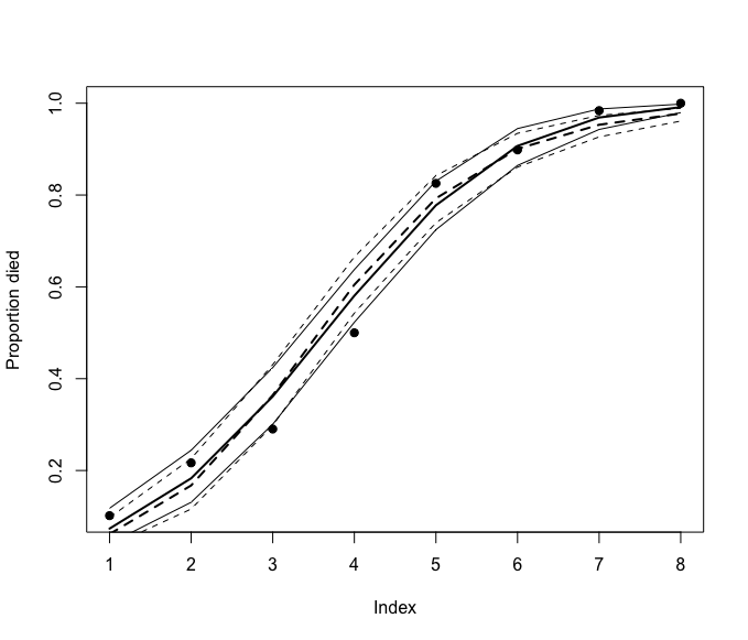
Figure 6: Fitted and observed proportions (– Skewed Probit, - - Probit) with $95\%$ credible intervals

6.2 Heart disease data

We will use the Cleveland data obtained by Robert Detrano from the V.A. Medical Center, Long Beach and Cleveland Clinic Foundation.

The response is a binary observation indicating the occurrence of a $>50\%$ diameter narrowing in an angiography. Various covariates are available in this data and we will use a subset of these namely, gender (male/female), type of chest pain (1 - typical angina, 2 - atypical angina, 3 - non-anginal pain, 4 - asymptomatic), resting blood pressure, the slope of the peak exercise ST segment (1 - upsloping, 2 - flat, 3 - down sloping), the number of colored vessels by fluoroscopy and the results from the thallium heart scan (3 - normal, 6 - fixed defect, 7 - reversable defect). We centered the two continuous covariates, resting heart rate and the number of colored vessels by fluoroscopy. Further details can be found in [18].

There are 297 subjects with complete information in the dataset of which 137 experienced the event of $>50\%$ diameter narrowing in an angiography. We fit a skewed-probit regression model to explain the probability of the event based on the values of the covariates similar to [23]. In [23] divergent results were obtained based on different estimation frameworks, namely maximum likelihood estimation, bootstrap bias correction, Jeffrey’s prior, generalized information matrix prior and Cauchy prior penalized frameworks. The inconsistent results could be attributed to the issues we mentioned in this paper, since all these estimation methods were developed for the skewed-probit regression model without the good standardization, based on the skewness parameter $\alpha$ and defined using the classical intercept.

Also, there is a lack of information on the skewness in binary data. The consequence is thus that various values of the skewness could be supported. This setup necessitates the need for the PC prior of the skewness, so that we will use probit regression unless the data strongly supports skewed probit regression.

Here, we can use the PC prior (10) for the skewness and the quantile intercept from Section 2.2. All quantitative covariates are centered. The results are given in Table 4.

	Posterior mean	$\mathbf{95\%}$ credible interval
Quantile Intercept ($q$)	$0.045$	$(0.006;0.184)$
Gender (male)	$1.025$	$(0.605;1.461)$
Type of chest pain (2)	$0.198$	$(-0.538;0.942)$
Type of chest pain (3)	$-0.074$	$(-0.732;0.590)$
Type of chest pain (4)	$1.288$	$(0.673;1.920)$
Resting heart rate	$0.016$	$(0.005;0.027)$
Slope of the peak exercise (2)	$1.027$	$(0.637;1.452)$
Slope of the peak exercise (3)	$0.791$	$(0.059;1.540)$
Number of colored vessels	$0.704$	$(0.477;0.945)$
Skewness $(\gamma_{1})$	$0.02$	$(-0.214;0.235)$

Table 4: Results for the Cleveland heart disease data

From the estimate of $\gamma_{1}$ in Table 4 we deduce that the skewness is not supported by the data and a probit regression model could be sufficient. We did the analysis using probit regression and the inference is very similar. This result coincides with most of the results in [23]. The posterior densities (and prior densities in dashed) of the skewness, $\gamma_{1}$, and quantile intercept, $q$, are presented in Figure 7.

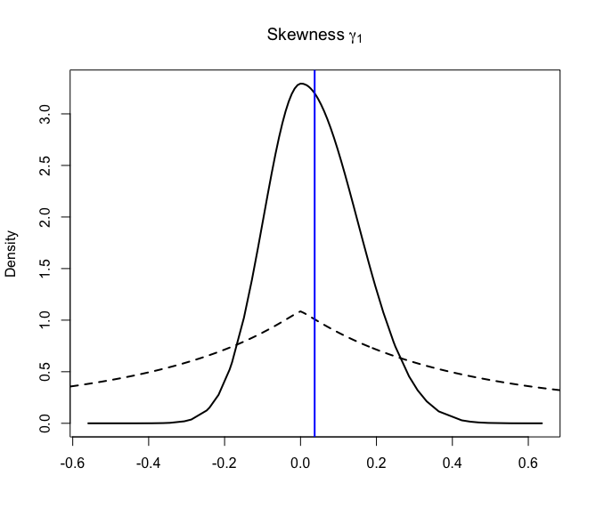
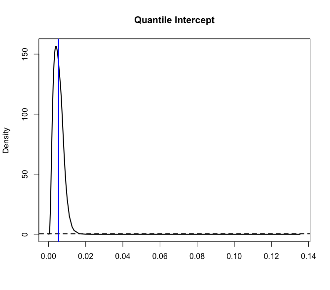
Figure 7: Posterior (prior - dashed) density of the skewness $\gamma_{1}$ (left) and quantile intercept $q$ (right) with the corresponding point estimates (vertical line)

We also see that being a male, having asymptomatic chest pain, higher resting heart rate, a flat or downwards slope of the peak exercise ST segment and more colored vessels by fluoroscopy, all contribute to a higher probability of the event under investigation, i.e. $>50\%$ diameter narrowing in an angiography.

The posterior densities (and prior densities in dashed) of the fixed effects are presented in Figure 8.

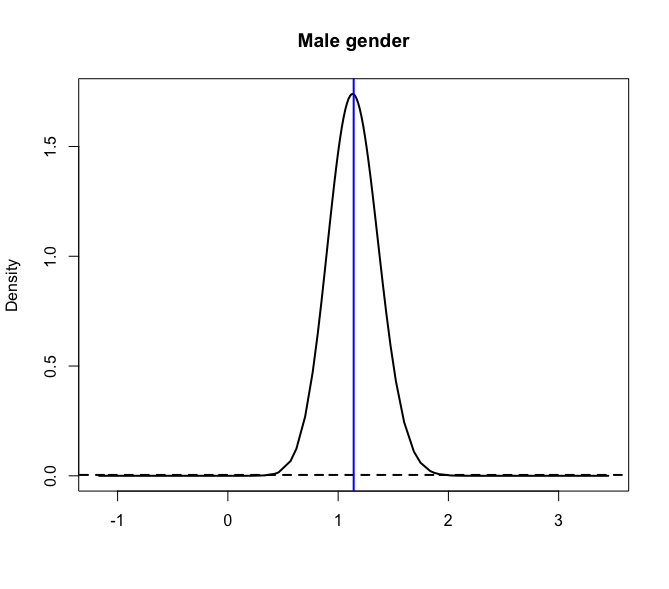
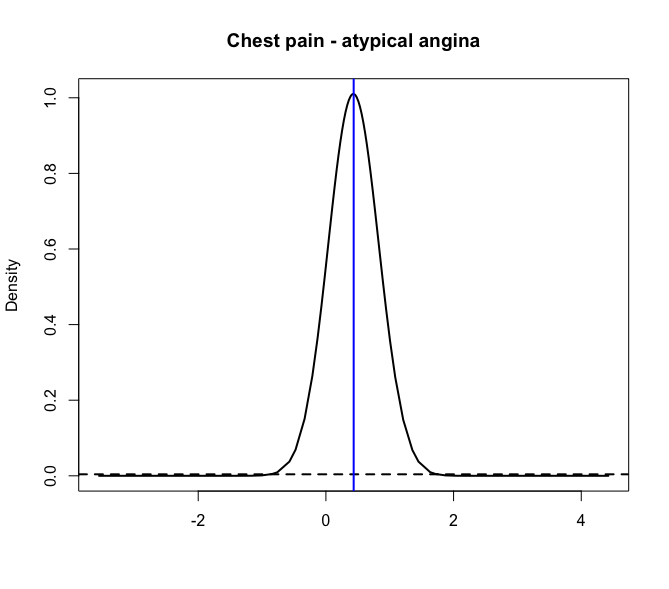
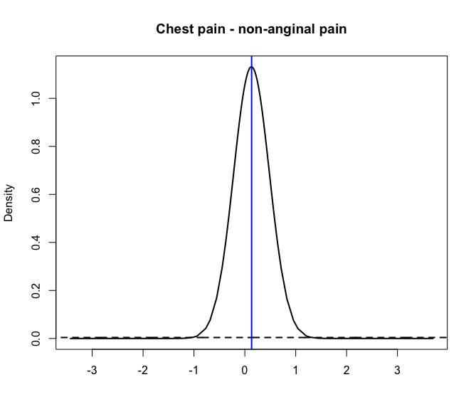
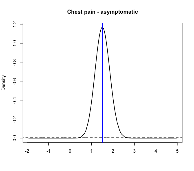
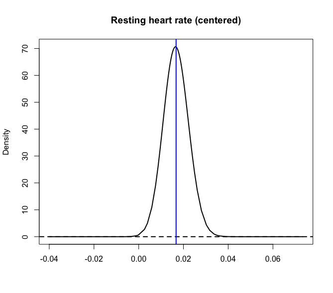
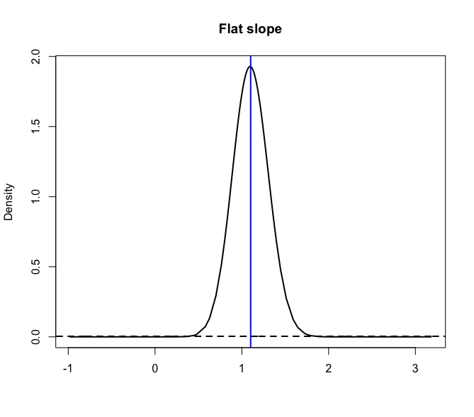
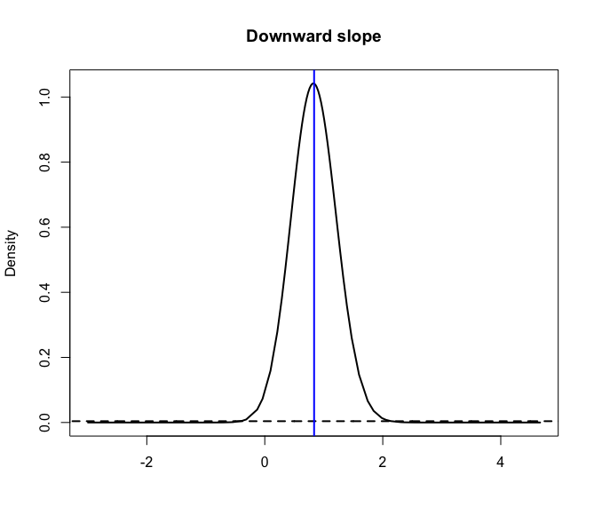
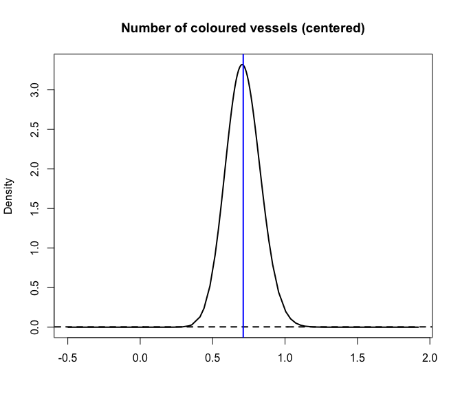
Figure 8: Posterior (prior - dashed) densities of the fixed effects with the corresponding point estimate (vertical line)

We calculated the marginal log-likelihoods for the probit and skewed-probit models to be $-150.62$ and $-158.41$, respectively, indicating that the probit model is preferred by the data. Both models achieved a correct classification percentage of $84.55\%$, on a $50\%$ holdout sample.

6.3 Wines data

This section illustrates the new results when the response variable is continuous and assumed to follow a skew-normal distribution. As mentioned in Section 3, the results derived in this paper hold for skewed-probit models, as well as skew-normal regression models. We use the wines dataset from [4], where the acidity of the wine is assumed to follow a skew-normal distribution as illustrated in Figure 9, where we see the tail behaviour is correctly captured by the fitted Gaussian density, but not the skewness. The mean acidity (not the location parameter) is modelled using the type of wine, sugar content and pH level as covariates (after backwards elimination). We assign PC priors for the precision [31] as well as skewness (10). The results are given in Table 5. The marginal log-likelihood for the skew-normal model is $-722.21$ and for the Gaussian model it is $-724.59$.

	Posterior mean	$\mathbf{95\%}$ credible interval
Intercept	$77.053$	$(73.824;80.252)$
Wine (Grignolino)	$5.088$	$(0.478;9.693)$
Wine (Barbera)	$23.613$	$(19.003;28.280)$
Sugar	$3.118$	$(1.150;5.080)$
pH	$-8.350$	$(-10.122;-6.574)$
Skewness $(\gamma_{1})$	$0.439$	$(0.128;0.702)$
Precision for the data	$0.008$	$(0.006;0.009)$

Table 5: Results for the wines data

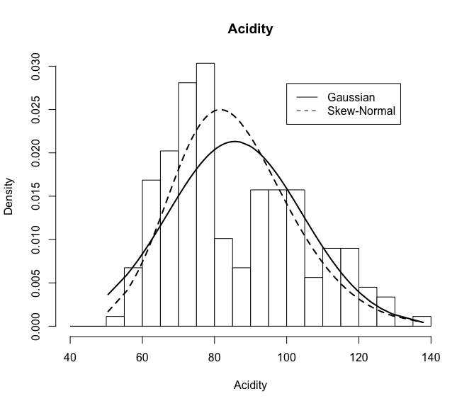
Figure 9: Histogram with model-based Gaussian curve and skew-normal curve

7 DISCUSSION

The use of skew-symmetric distributions or links is popular due to the perceived flexibility inherited through the extra parameter that controls the skewness. The skew normal skewness parameter in particular, poses various challenges in the inference thereof. As we set out with the initial aim to derive the penalizing complexity prior for the skewness, we realized that there are various other issues that we could not found addressed in the literature. It is apparent that with the generalizing to skew-symmetric distributions and links from the symmetric counterparts, various fundamental concepts have gone amiss.

Here we rectify the formulation of the intercept in the linear predictor of all skew-symmetric links, firstly to ensure that it behaves as an intercept and secondly due to the confounding with the skewness parameter and fixed effects. We also show that the popular method of standardizing the skewed link function by inheriting the parameter values of the symmetric link, fundamentally changes the way the link function maps the data to the linear predictor, and we provide an anchored standardization approach. We believe that many of the contradicting works in this area can be attributed to the inappropriate use of the classical intercept and parameter-based standardization, instead of property-based standardization. In skew-symmetric regression models, we formulate the regression model based on the mean, instead of the location parameter.

After the fundamental corrections to the formulation of the skewed-probit link, the penalizing complexity prior for the skewness was derived. One particular advantage of this prior is that it is invariant to reparameterizations of the skewness parameter. In light of this, we implemented the PC prior for the skewness in R-INLA [29] for use by others. We noted, expectedly, that binary data (or with few trials) does not provide information about the skewness, and we thus advise against the use of the skewed-probit link for data with a small number of trials. We advocate the use of the PC prior even more feverently because of this feature, since the PC prior will contract to the simpler probit link instead of providing an incorrect unreliable estimate of the skewness. Other inferential frameworks might not be able to ensure this contraction in the absence of convincing evidence from the data about the necessary skewness, and could lead to unfounded complicated models.

We hope that the issues raised and addressed here will improve the inference of the skewed probit model (and more broadly the skew-symmetric links and likelihoods) and provide insights into the fundamental considerations necessary when distributions or links are generalized.

Appendix

We give here a small example for how to do skew probit regression in R-INLA. In the code below, the unusual statement is remove.names="(Intercept)" which remove the intercept in the formula after doing the expansion of factors in the model. We need this as we replace the traditional intercept with the quantile intercept in the link, and the expansion of factors depends on the presence or not, of an intercept in the model.

library(INLA)
n = 200
Ntrials = 200
x = rnorm(n, sd = 0.5)
eta = x
skew <- 0.5
prob = inla.link.invsn(eta, skew = skew, intercept = 0.75)
y = rbinom(n, size = Ntrials,  prob = prob)
r = inla(y ~ 1 + x,
    family = "binomial",
    data = data.frame(y, x),
    Ntrials = Ntrials,
    control.fixed = list(remove.names = "(Intercept)",
                         prec = 1),
    control.family = list(
        control.link = list(model = "sn",
                            hyper = list(
                                skew = list(param = 10)))))
summary(r)

References

- Arellano-Valle et al., [2007] Arellano-Valle, R., Bolfarine, H., and Lachos, V. (2007). Bayesian inference for skew-normal linear mixed models. Journal of Applied Statistics, 34(6):663–682.
- Azevedo et al., [2011] Azevedo, C. L., Bolfarine, H., and Andrade, D. F. (2011). Bayesian inference for a skew-normal irt model under the centred parameterization. Computational Statistics & Data Analysis, 55(1):353–365.
- Azzalini, [1985] Azzalini, A. (1985). A class of distributions which includes the normal ones. Scandinavian journal of statistics, pages 171–178.
- Azzalini, [2013] Azzalini, A. (2013). The skew-normal and related families, volume 3. Cambridge University Press.
- Azzalini and Arellano-Valle, [2013] Azzalini, A. and Arellano-Valle, R. B. (2013). Maximum penalized likelihood estimation for skew-normal and skew-t distributions. Journal of Statistical Planning and Inference, 143(2):419–433.
- Azzalini and Capitanio, [2003] Azzalini, A. and Capitanio, A. (2003). Distributions generated by perturbation of symmetry with emphasis on a multivariate skew t-distribution. Journal of the Royal Statistical Society: Series B (Statistical Methodology), 65(2):367–389.
- Bayes and Branco, [2007] Bayes, C. L. and Branco, M. D. (2007). Bayesian inference for the skewness parameter of the scalar skew-normal distribution. Brazilian Journal of Probability and Statistics, pages 141–163.
- Bazán et al., [2010] Bazán, J. L., Bolfarine, H., and Branco, M. D. (2010). A framework for skew-probit links in binary regression. Communications in Statistics-Theory and Methods, 39(4):678–697.
- Bazán et al., [2006] Bazán, J. L., Branco, M. D., Bolfarine, H., et al. (2006). A skew item response model. Bayesian analysis, 1(4):861–892.
- Bliss, [1935] Bliss, C. I. (1935). The calculation of the dosage-mortality curve. Annals of Applied Biology, 22(1):134–167.
- Cabras et al., [2012] Cabras, S., Racugno, W., Castellanos, M. E., and Ventura, L. (2012). A matching prior for the shape parameter of the skew-normal distribution. Scandinavian Journal of Statistics, 39(2):236–247.
- Canale et al., [2016] Canale, A., Kenne Pagui, E. C., and Scarpa, B. (2016). Bayesian modeling of university first-year students’ grades after placement test. Journal of Applied Statistics, 43(16):3015–3029.
- Castro et al., [2013] Castro, L. M., Martín, E. S., and Arellano-Valle, R. B. (2013). A note on the parameterization of multivariate skewed-normal distributions. Brazilian Journal of Probability and Statistics, pages 110–115.
- Chen et al., [1999] Chen, M.-H., Dey, D. K., and Shao, Q.-M. (1999). A new skewed link model for dichotomous quantal response data. Journal of the American Statistical Association, 94(448):1172–1186.
- Collet, [2003] Collet, D. (2003). Modelling Binary Data. , 2nd ed. Chapman & Hall/CRC, Boca Raton , FL.
- Czado and Santner, [1992] Czado, C. and Santner, T. J. (1992). The effect of link misspecification on binary regression inference. Journal of statistical planning and inference, 33(2):213–231.
- Dette et al., [2018] Dette, H., Ley, C., and Rubio, F. (2018). Natural (non-) informative priors for skew-symmetric distributions. Scandinavian Journal of Statistics, 45(2):405–420.
- Dua and Graff, [2017] Dua, D. and Graff, C. (2017). UCI machine learning repository.
- Firth, [1993] Firth, D. (1993). Bias reduction of maximum likelihood estimates. Biometrika, 80(1):27–38.
- Genton, [2004] Genton, M. G. (2004). Skew-elliptical distributions and their applications: a journey beyond normality. CRC Press.
- Genton and Zhang, [2012] Genton, M. G. and Zhang, H. (2012). Identifiability problems in some non-gaussian spatial random fields. Chilean Journal of Statistics, 3(2):171–179.
- Hallin et al., [2014] Hallin, M., Ley, C., et al. (2014). Skew-symmetric distributions and fisher information: the double sin of the skew-normal. Bernoulli, 20(3):1432–1453.
- Lee and Sinha, [2019] Lee, D. and Sinha, S. (2019). Identifiability and bias reduction in the skew-probit model for a binary response. Journal of Statistical Computation and Simulation, 89(9):1621–1648.
- Liseo, [1990] Liseo, B. (1990). The skew-normal class of densities: inferential aspects from a bayesian viewpoint. Statistica, 50:59–70.
- Liseo and Loperfido, [2006] Liseo, B. and Loperfido, N. (2006). A note on reference priors for the scalar skew-normal distribution. Journal of Statistical Planning and Inference, 136(2):373–389.
- Maghami et al., [2020] Maghami, M. M., Bahrami, M., and Sajadi, F. A. (2020). On bias reduction estimators of skew-normal and skew-t distributions. Journal of Applied Statistics, pages 1–23.
- O’hagan and Leonard, [1976] O’hagan, A. and Leonard, T. (1976). Bayes estimation subject to uncertainty about parameter constraints. Biometrika, 63(1):201–203.
- Otiniano et al., [2015] Otiniano, C., Rathie, P., and Ozelim, L. (2015). On the identifiability of finite mixture of skew-normal and skew-t distributions. Statistics & Probability Letters, 106:103–108.
- Rue et al., [2009] Rue, H., Martino, S., and Chopin, N. (2009). Approximate Bayesian inference for latent Gaussian models by using integrated nested laplace approximations. Journal of the Royal Statistical Society: Series B (Statistical Methodology), 71(2):319–392.
- Sartori, [2006] Sartori, N. (2006). Bias prevention of maximum likelihood estimates for scalar skew normal and skew t distributions. Journal of Statistical Planning and Inference, 136(12):4259–4275.
- Simpson et al., [2017] Simpson, D., Rue, H., Riebler, A., Martins, T. G., Sørbye, S. H., et al. (2017). Penalising model component complexity: A principled, practical approach to constructing priors. Statistical Science, 32(1):1–28.