Robust generation of logical qubit singlet states with reverse engineering and optimal control with spin qubits

Abstract

A protocol is proposed to generate singlet states of three logical qubits constructed by pairs of spins. Single and multiple operations of logical qubits are studied for the construction of an effective Hamiltonian, with which robust control fields are derived with invariant-based reverse engineering and optimal control. Moreover, systematic errors are further compensated by periodic modulation for better robustness. Furthermore, resistance to decoherence of the protocol is also shown with numerical simulations. Therefore, the protocol may provide useful perspectives for generations of logical qubit entanglement in spin systems.

I Introduction

Quantum entanglement is one of the most fascinating properties of quantum mechanics. It has been shown in the past decades that different types of entangled states, e.g., the Bell states BellPhysics1 , Greenberger-Horne-Zeilinger (GHZ) states Greenberger and W states DurPRA62 can be alternative candidates in testing non-locality CabelloPRA65 and realizing quantum information processing (QIP) BennettNat404 . As entangled states have been widely applied in the field of QIP, understanding of entanglement is gradually enhanced. Thus, increasing interests have been recently attracted by generalized entangled states, including high-dimensional entangled states TureciPRB75 ; LGWPRA76 ; LWAPRA83 ; SXQPRA89 ; SCPRA93 , logical qubit entangled states FrowisPRL106 ; MunroNP6 ; FrowisPRA85 ; ZLPRA92 , and macroscopic entangled state RDPRA102 ; CYHarxiv .

High-dimensional entangled states are entangled states defined in Hilbert spaces with more than two dimensions. Compared with typical two-dimensional entangled states, high-dimensional entangled states have shown stronger violations of local realism, larger information capability and better security in quantum key distribution KaszlikowskiPRL85 ; BourennanePRA64 ; BrubPRL88 ; CerfPRL88 . The singlet state is an important kind of high-dimensional entangled states. As a generalization of Bell singlet state $(|01\rangle-|10\rangle)/\sqrt{2}$, a $D$-dimensional ($D=3,4,5,...$) singlet state encoded on $D$ qubits with $D$-dimensional basis is defined as CabelloPRL89

$$|S_{D}\rangle=\frac{1}{\sqrt{D!}}\sum\limits_{\nu}(-1)^{\tau(\nu)}|\nu\rangle.$$ (1)

In Eq. (1), $\nu$ is a permutation of $0,1,2,...,D-1$, and $\tau(\nu)$ is the least times required to make transpositions of pairs of elements for the canonical order, i.e., $0,1,2,...,D-1$. Singlet states have shown violations of Bell inequalities MerminPRD22 , and can be used in solving various problems CabelloPRL89 ; CabelloJMO50 . These attractive features have encouraged many researchers to study high-fidelity generations of singlet states in different physical systems during the past few years SHPRA95 ; SXQPRA85 ; CXPRA96 ; SXQPRA94 ; CXPRA98 ; SXQNJP12 .

In addition, logical qubit entangled states are entangled states encoded on logical qubits constructed by a group of physical qubits HMKPRL99 ; ShawPRA78 ; ZJPRL109 ; KapitPRL120 . Logical qubit entangled states have potential to build up decoherence-free subspaces against collective decoherence WaltonPRL91 ; SYBSR5 ; ZLSR6 . When a part of physical qubits suffer from decoherence, errors may be corrected through feedback control or entanglement concentration and purification HLNP15 ; QCQIP14 ; WXQIP17 . To date, various types of logical qubit entangled states, e.g., logical Bell states ZLSR62 and concatenated GHZ states KestingPRA88 ; LHNP8 , have been investigated with a lot of advantages shown. How to realize high-fidelity preparations of these states is now a question attracting continuously attention.

Spin systems are promising platforms with long coherence time, good scalability and operability XZLRMP85 , which have been exploited in generations of typical entangled states such as the Bell states, GHZ states and W states PaulPRA94 ; StefanatosPRA99 ; YXTPRA97 ; JLPRA79 ; CJPRA95 ; JYPRA99 ; KYHPRA100 . To realize scalable quantum information processing, it is essential to expand results of protocols PaulPRA94 ; StefanatosPRA99 ; YXTPRA97 ; JLPRA79 ; CJPRA95 ; JYPRA99 ; KYHPRA100 , and study generations of multi-dimensional entanglement. However, in contrast to research in atomic systems SHPRA95 ; SXQPRA85 ; CXPRA96 ; SXQPRA94 ; CXPRA98 ; SXQNJP12 , there are still not many works in spin systems for generations of high-dimensional entangled states including singlet states with more than three qubits. One of the reasons is that a single spin has only two natural states $|\uparrow\rangle$ and $|\downarrow\rangle$. Considering features of logical qubits, they provide extensible way to encode quantum information in spin systems, and may be more robust against collective decoherence FrowisPRL106 ; FrowisPRA85 . From this point, we propose a protocol to generate logical qubit singlet states in the spin system. We analyze the dynamics of a system with three logical qubits constructed by pairs of spins, and derive Hamiltonians for single- and multi-qubit operations. Based on the results, robust control fields are derived based on invariant-based reverse engineering CXPRA86 ; ImpensPRA96 ; OdelinRMP91 ; IbanezPRA87 ; TorronteguiPRA89 ; KYHPRA101 and optimal control RuschhauptNJP14 ; DaemsPRL111 ; DammePRA95 ; DammePRA96 ; LXJPRA88 ; KYHPRA102 . Moreover, we further reduce the influence of systematic errors by periodic modulation. Numerical simulations show the protocol holds better robustness than protocols with time-independent couplings and with only reverse engineering. Influence of decoherence is also taken into account with reported coherence time of spins XZLRMP85 , the results demonstrate the protocol can generate singlet states with acceptable fidelities in the presence of decoherence. With current technology in quantum dots and nuclear magnetic resonance (NMR) systems, physical implementation of the protocol is feasible. The systematic errors discussed in the protocol are also relevant to realistic physical systems. Therefore, the protocol may be helpful to generations of singlet states in spin systems.

II Lewis-Riesenfeld invariant theory

Let us first briefly introduce the Lewis-Riesenfeld invariant theory LewisJMP10 . We consider a quantum system with Hamiltonian $H(t)$. Introducing an invariant Hermitian operator $I(t)$, satisfying ($\hbar=1$)

$$\dot{I}(t)+i[H(t),I(t)]=0,$$ (2)

an arbitrary solution $|\Psi(t)\rangle$ of time-dependent Schrödinger equation $i|\dot{\Psi}(t)\rangle=H(t)|\Psi(t)\rangle$ can be expanded by eigenstates of $I(t)$ as

$$|\Psi(t)\rangle=\sum\limits_{k}C_{k}e^{i\alpha_{k}}|\Phi_{k}(t)\rangle.$$ (3)

Here, $|\Phi_{k}(t)\rangle$ is the $k$-th eigenstate of $I(t)$, and $C_{k}=\langle\Phi_{k}(0)|\Psi(0)\rangle$ denotes the corresponding coefficient. $\alpha_{k}(t)$ is the Lewis-Riesenfeld phase acquired by $|\Phi_{k}(t)\rangle$, obeying

$$\dot{\alpha}_{k}(t)=i\langle\Phi_{k}(t)|\dot{\Phi}_{k}(t)\rangle-\langle\Phi_{k}(t)|H(t)|\Phi_{k}(t)\rangle,$$ (4)

with $\alpha_{k}(0)=0$ and the initial time $t_{i}=0$. In practice, one can realize construction of dynamic invariants and invariant-based reverse engineering with the help of Lie algebra, which are briefly introduced in Appendix B.

III Physical model and Hamiltonian

We now introduce the physical model for generations of singlet states of three logical qubits. Considering a system with three pairs of spins, which are used as three logical qubits, named $q_{1}$, $q_{2}$ and $q_{3}$, respectively. The spins in pair $q_{j}$ ($j=1,2,3$) are denoted by $q_{j_{1}}$ and $q_{j_{2}}$, respectively. Generally, state of each logical qubit can be described with a Bell-state basis as

$$|0\rangle=\frac{1}{\sqrt{2}}(|\uparrow\uparrow\rangle+|\downarrow\downarrow\rangle),\ |1\rangle=\frac{1}{\sqrt{2}}(|\uparrow\downarrow\rangle+|\downarrow\uparrow\rangle),$$ (5)

$$|2\rangle=\frac{1}{\sqrt{2}}(|\uparrow\uparrow\rangle-|\downarrow\downarrow\rangle),\ |3\rangle=\frac{1}{\sqrt{2}}(|\uparrow\downarrow\rangle-|\downarrow\uparrow\rangle).$$

The singlet state to be prepared reads $|\Psi_{s}\rangle=(|012\rangle+|120\rangle+|201\rangle-|102\rangle-|210\rangle-|021\rangle)/\sqrt{6}$. When spins $q_{j_{1}}$ and $q_{j_{2}}$ interact with each other through Heisenberg exchange interactions with Hamiltonian YXTPRA97 ; ZajacSci359 ; RussPRB97 ; VargasPRB100

$$H_{j}=\sum\limits_{\jmath=x,y,z}\frac{J_{\jmath j}}{4}\sigma_{\jmath}^{(q_{j_{1}})}\otimes\sigma_{\jmath}^{(q_{j_{2}})},$$ (6)

we can obtain a single-qubit operation for logical qubit $q_{j}$ in the Bell-state basis as

$$H_{j}=\frac{1}{4}[(J_{xj}-J_{yj}+J_{zj})|0\rangle_{j}\langle 0|+(J_{xj}+J_{yj}-J_{zj})|1\rangle_{j}\langle 1|$$ (7)

$$+(-J_{xj}+J_{yj}+J_{zj})|2\rangle_{j}\langle 2|-(J_{xj}+J_{yj}+J_{zj})|3\rangle_{j}\langle 3|],$$

where $J_{\jmath j}$ ($\jmath=x,y,z$) is the strength of exchange interaction in $\jmath$-direction. From Eq. (7), we find that $H_{j}$ only induces energy splits among different Bell states in the Bell-state basis of logical qubit $q_{j}$. Thus, if we encode quantum information on states $|0\rangle$, $|1\rangle$ and $|2\rangle$ in the generation of three-logical-qubit singlet state, state $|3\rangle$ is dynamically decoupled to the considered subspace through $H_{j}$.

To obtain entanglement of logical qubits $\{q_{j}\}$, we also require multi-qubit operations between each pair of logical qubits. Here, we construct a two-qubit operation for logical qubits $q_{1}$ and $q_{2}$ as an example for constructions of multi-qubit operations. We assume that two spins in pair $(q_{1_{\iota}},q_{2_{\iota^{\prime}}})$ ($\iota,\iota^{\prime}=1,2$) interact with each other through exchange interactions with the same strengths $\{g_{\jmath}(t)|\jmath=x,y,z\}$ in three different directions, such that the Hamitonian can be written by YXTPRA97 ; ZajacSci359 ; RussPRB97 ; VargasPRB100

$$H_{12}(t)=\sum\limits_{\jmath=x,y,z}\sum\limits_{\iota,\iota^{\prime}=1,2}\frac{g_{\jmath}(t)}{4}\sigma_{\jmath}^{(q_{1_{\iota}})}\otimes\sigma_{\jmath}^{(q_{2_{\iota^{\prime}}})}.$$ (8)

$H_{12}$ can described by a product Bell-state basis of $q_{1}$ and $q_{2}$ as

$$H_{12}(t) =H_{ex}^{(12)}(t)+H_{dp}^{(12)}(t),$$ (9)

$$H_{ex}^{(12)}(t) =g_{x}(t)|01\rangle_{12}\langle 10|+g_{y}(t)|12\rangle_{12}\langle 21|+g_{z}(t)|02\rangle_{12}\langle 20|+\mathrm{H.c.},$$

$$H_{dp}^{(12)}(t) =g_{x}(t)|00\rangle_{12}\langle 11|-g_{y}(t)|11\rangle_{12}\langle 22|+g_{z}(t)|00\rangle_{12}\langle 22|+\mathrm{H.c.}$$

According to Eq. (9), $H_{12}(t)$ can be divided into two parts. $H_{ex}^{(12)}(t)$ exchanges the states of logical qubits $q_{1}$ and $q_{2}$, while $H_{du}^{(12)}(t)$ only works when two logical qubits in the same state in the Bell-state basis. With similar deviations to the two-qubit operation of logical qubits $q_{1}$ and $q_{3}$ ($q_{2}$ and $q_{3}$), we can also obtain $H_{13}(t)$ ($H_{23}(t)$) with similar form of Eq. (9). Consequently, if we prepare the system in state $|012\rangle$ initially, the Hamiltonian component

$$H_{dp}(t)=\sum\limits_{j<j^{\prime}}H_{dp}^{(jj^{\prime})}(t),$$ (10)

does not work, thus the evolution can be studied in a six-dimensional subspace spanned by

$$|\psi_{1}\rangle=|012\rangle,\ |\psi_{2}\rangle=|102\rangle,\ |\psi_{3}\rangle=|120\rangle,\ |\psi_{4}\rangle=|210\rangle,\ |\psi_{5}\rangle=|201\rangle,\ |\psi_{6}\rangle=|021\rangle.$$ (11)

In this subspace, the singlet state $|\Psi_{s}\rangle$ can be described by a simple form as

$$|\Psi_{s}\rangle=\frac{1}{\sqrt{6}}\sum\limits_{n=1}^{6}(-1)^{n+1}|\psi_{n}\rangle,$$ (12)

and the multi-qubit Hamiltonian can also be simplified as

$$H_{mu}(t)=\sum\limits_{j<j^{\prime}}H_{ex}^{(jj^{\prime})}(t)=g(t)(|\psi_{1}\rangle+|\psi_{3}\rangle+|\psi_{5}\rangle)(\langle\psi_{2}|+\langle\psi_{4}|+\langle\psi_{6}|)+\mathrm{H.c.},$$ (13)

with isotropic interactions $g_{x}(t)=g_{y}(t)=g_{z}(t)=g(t)$ RussPRB97 ; VargasPRB100 .

Since the singlet state $|\Psi_{s}\rangle$ is an eigenstate of the Hamiltonian $H_{mu}(t)$, the generation of $|\Psi_{s}\rangle$ from initial state $|\psi_{1}\rangle$ is impossible with only $H_{mu}(t)$. Thus, assistance of the single-qubit Hamiltonian $\{H_{j}|j=1,2,3\}$ is important to the protocol. To construct an effective Hamiltonian towards the target state $|\Psi_{s}\rangle$, we select interaction strengths in $\{H_{j}\}$ as YXTPRA97

$$J_{x1}=J_{z1}=J_{x2}=J_{y2}=J_{y3}=J_{z3}=J,\ J_{y1}=J_{z2}=J_{x3}=0.$$ (14)

In this case, Hamiltonian of the total system in the rotation frame of $R(t)=\exp(-i\sum_{j=1}^{3}H_{j}t)$ reads

$$H_{R}(t)=g(t)e^{-iJt}(e^{i3Jt}|\psi_{1}\rangle+|\psi_{3}\rangle+|\psi_{5}\rangle)(\langle\psi_{2}|+\langle\psi_{4}|+\langle\psi_{6}|)+\mathrm{H.c.}$$ (15)

By setting

$$g(t)=[2g_{1}(t)\sin(2Jt)+\sqrt{2}g_{2}(t)\sin(Jt)]/\sqrt{3},$$ (16)

we obtain an effective Hamiltonian as

$$H_{e}(t)=ig_{1}(t)|\phi_{1}\rangle\langle\phi_{2}|-ig_{2}(t)|\phi_{3}\rangle\langle\phi_{2}|+\mathrm{H.c.},$$ (17)

with

$$|\phi_{1}\rangle=|\psi_{1}\rangle,\ |\phi_{2}\rangle=\frac{1}{\sqrt{3}}(|\psi_{2}\rangle+|\psi_{4}\rangle+|\psi_{6}\rangle),\ |\phi_{3}\rangle=\frac{1}{\sqrt{2}}(|\psi_{3}\rangle+|\psi_{5}\rangle),$$ (18)

under the condition $|g_{1}(t)|,|g_{2}(t)|\ll J$. In the next section, we would show that invariant-based reverse engineering can be exploited to construct evolution path for the generation of the singlet state $|\Psi_{s}\rangle$ with the effective Hamiltonian $H_{e}(t)$.

IV Construction of evolution path via invariant-based reverse engineering

Now, let us design the control functions $g_{1}(t)$ and $g_{2}(t)$ via invariant-based reverse engineering to obtain the singlet state $|\Psi_{s}\rangle$. According to Eq. (17), the effective Hamiltonian can be decomposed as

$$H_{e}(t)=g_{1}(t)G_{1}+g_{2}(t)G_{2}+0\times G_{3},$$ (19)

with

$$G_{1}=\left[\begin{array}[]{ccc}0&\ i&\ 0\\ -i&\ 0&\ 0\\ 0&\ 0&\ 0\\ \end{array}\right],\ G_{2}=\left[\begin{array}[]{ccc}0&\ 0&\ 0\\ 0&\ 0&\ i\\ 0&\ -i&\ 0\\ \end{array}\right],\ G_{3}=\left[\begin{array}[]{ccc}0&\ 0&\ i\\ 0&\ 0&\ 0\\ -i&\ 0&\ 0\\ \end{array}\right],$$ (20)

being generators of special orthogonal Lie algebra so(3) obeying commutation relations

$$[G_{1},G_{2}]=iG_{3},\ [G_{2},G_{3}]=iG_{1},\ [G_{3},G_{1}]=iG_{2}.$$ (21)

As invariants can be always constructed by generators of Lie algebra TorronteguiPRA89 , we here consider an invariant in form of

$$I(t)=\lambda_{1}(t)G_{1}+\lambda_{2}(t)G_{2}+\lambda_{3}(t)G_{3},$$ (22)

with $\lambda_{1}(t)$, $\lambda_{2}(t)$ and $\lambda_{3}(t)$ being three real time-dependent coefficients. Substituting the invariant $I(t)$ in Eq. (22) and the effective Hamiltonian $H_{e}(t)$ in Eq. (19) into Eq. (2), we obtain

$$\dot{\lambda}_{1}=g_{2}\lambda_{3},\ \dot{\lambda}_{2}=-g_{1}\lambda_{3},\ \dot{\lambda}_{3}=g_{1}\lambda_{2}-g_{2}\lambda_{1}.$$ (23)

As the rank of the three equations in Eq. (23) is 2, a constraint equation can be derived as $\lambda_{1}^{2}+\lambda_{2}^{2}+\lambda_{3}^{2}=\mathrm{Const.}$ A simple way to parameterize $\lambda_{1}(t)$, $\lambda_{2}(t)$ and $\lambda_{3}(t)$ is using spherical coordinates for a unit sphere as

$$\lambda_{1}=\cos\theta\cos\beta,\ \lambda_{2}=\cos\theta\sin\beta,\ \lambda_{3}=\sin\theta.$$ (24)

Consequently, the control functions can be reversely solved from Eq. (23) as

$$g_{1}(t)=\dot{\theta}\sin\beta-\dot{\beta}\cot{\theta}\cos\beta,\ g_{2}(t)=-\dot{\theta}\cos\beta-\dot{\beta}\cot{\theta}\sin\beta.$$ (25)

In addition, eigenstates of the invariant $I(t)$ can be derived as

$$|\Phi_{0}(t)\rangle=\left[\begin{array}[]{c}\cos\theta\sin\beta\\ -\sin\theta\\ \cos\theta\cos\beta\\ \end{array}\right],\ |\Phi_{+}(t)\rangle=\left[\begin{array}[]{c}\sin\theta\sin\beta+i\cos\beta\\ \cos\theta\\ \sin\theta\cos\beta-i\sin\beta\\ \end{array}\right],\ |\Phi_{-}(t)\rangle=\left[\begin{array}[]{c}\sin\theta\sin\beta-i\cos\beta\\ \cos\theta\\ \sin\theta\cos\beta+i\sin\beta\\ \end{array}\right]\$$ (26)

corresponding to eigenvalues 0, 1 and -1, respectively. The Lewis-Riesenfeld phase acquired by $|\Phi_{0}(t)\rangle$ and $|\Phi_{\pm}(t)\rangle$ respectively read

$$\alpha_{0}(t)=0,\ \ \alpha_{\pm}(t)=\int_{0}^{t}\pm 2\dot{\beta}(t^{\prime})\csc[\theta(t^{\prime})]dt^{\prime}.$$ (27)

When we consider boundary conditions as

$$\theta(0)=0,\ \beta(0)=\pi/2,\ \theta(T)=\pi/4,\ \beta(T)=\arcsin(\sqrt{3}/3),$$ (28)

with $T$ being the operation time, invariant-based engineering allows us to evolve the system from the initial state $|\Psi(0)\rangle=|\phi_{1}\rangle$ to the final state $|\Psi(T)\rangle=(|\phi_{1}\rangle-\sqrt{3}|\phi_{2}\rangle+\sqrt{2}|\phi_{3}\rangle)/\sqrt{6}=|\Psi_{s}\rangle$ along the eigenstate $|\Phi_{0}(t)\rangle$. Therefore, the construction of evolution path has been successfully completed via invariant-based reverse engineering.

V Selections of control parameters via optimal control theory

Although the evolution path has been constructed through invariant-based reverse engineering, the problem of selections of control parameters has not yet been settled. Since the evolution path $|\Phi_{0}(t)\rangle$ only requests constraints of parameters at boundary, there still a lot of choices for specific expressions of parameters. However, not all parameter selections can produce robust fields against optional errors. Thus, how to select parameters for high-fidelity control is a very important problem required to be considered. Fortunately, optimal control theory provides us a powerful tool to deal with the problem. Here, we consider that there exists errors of control function $g(t)$ as $\delta g(t)$. In this case, the faulty effective Hamiltonian reads

$$H_{e}^{\prime}(t)=i(1+\delta)g_{1}(t)|\phi_{1}\rangle\langle\phi_{2}|-i(1+\delta)g_{2}(t)|\phi_{3}\rangle\langle\phi_{2}|+\mathrm{H.c.}$$ (29)

To start the optimal strategy, we use time-dependent perturbation theory RuschhauptNJP14 ; YXTPRA97 to derive

$$|\Psi^{\prime}(T)\rangle \simeq|\Phi_{0}(T)\rangle-i\int_{0}^{T}dtU(T,t)H^{\prime}(t)|\Phi_{0}(t)\rangle$$ (30)

$$-\int_{0}^{T}dt\int_{0}^{t}dt^{\prime}U(T,t)H^{\prime}(t)U(t,t^{\prime})H^{\prime}(t^{\prime})|\Phi_{0}(t^{\prime})\rangle+\mathcal{O}(\delta^{3}),$$

where $|\Psi^{\prime}(t)\rangle$ is state of the system with systematic errors, $H^{\prime}(t)=\delta H_{e}(t)$ is the total perturbation Hamiltonian, and $U(t,t^{\prime})$ reads

$$U(t,t^{\prime})=\sum\limits_{k=0,\pm}e^{i[\alpha_{k}(t)-\alpha_{k}(t^{\prime})]}|\Phi_{k}(t)\rangle\langle\Phi_{k}(t^{\prime})|,$$ (31)

being the evolution operator of the system in time interval $[t^{\prime},t]$ without systematic errors. With the help of Eq. (30), the fidelity $F=|\langle\Psi^{\prime}(T)|\Psi_{s}\rangle|^{2}$ can be estimated as

$$F\simeq 1-\sum\limits_{k\neq 0}|\int_{0}^{T}e^{-i\alpha_{k}(t)}\langle\Phi_{k}(t)|H^{\prime}(t)|\Phi_{0}(t)\rangle dt|^{2},$$ (32)

with second order of $\delta$ being kept. Defining systematic error sensitivity as $Q_{s}=-\partial^{2}F/2\partial\delta^{2}$ RuschhauptNJP14 , we have

$$Q_{s}=2|\int_{0}^{T}(\dot{\beta}\cos\theta\sin\alpha+\dot{\theta}\cos\alpha)dt|^{2},$$ (33)

with $\alpha(t)=\alpha_{+}(t)$. Inspired by Ref. DaemsPRL111 , we consider a Fourier series of $\beta(t)$ as

$$\beta(t)=\beta(T)\mu(t)+\beta(0)[1-\mu(t)]+\kappa_{1}\sin[\pi\mu(t)]+\kappa_{2}\sin[2\pi\mu(t)],\ \mu(t)=[\theta(t)/\theta(T)]^{2}.$$ (34)

Considering the interpolation of $\theta(t)$ with boundary conditions shown in Eq. (28) and $\dot{\theta}(0)=\dot{\theta}(T)=0$ by using sine function as

$$\theta(t)=\frac{\pi}{4}\sin^{2}(\frac{\pi t}{2T}),$$ (35)

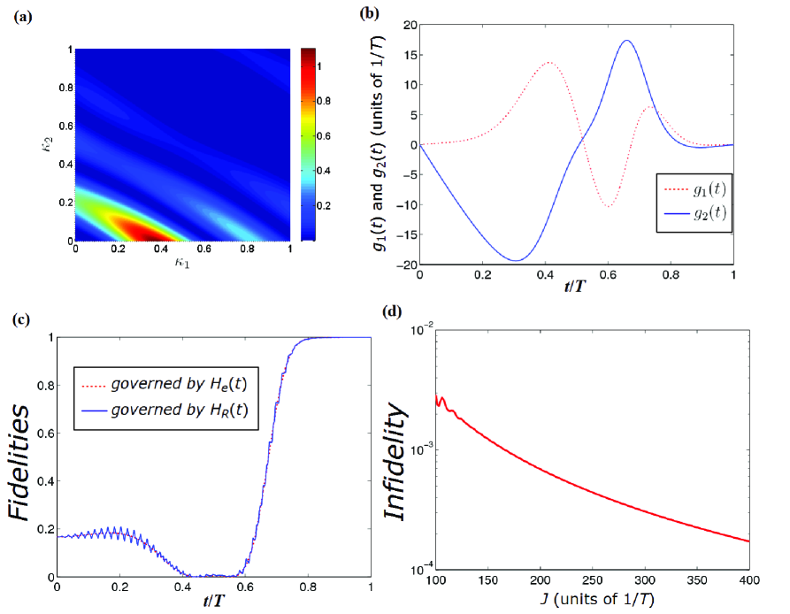
Figure 1: (a) $Q_{s}$ versus $\kappa_{1}$ and $\kappa_{2}$. (b) $g_{1}(t)$ and $g_{2}(t)$ versus $t/T$. (c) The fidelities $F=|\langle\Psi(t)|\Psi_{s}\rangle|^{2}$ of obtaining the singlet state $|\Psi_{s}\rangle$ versus $t/T$ with the effective Hamiltonian $H_{e}$ (red-dotted line) and the Hamiltonian $H_{R}(t)$ with $J=300/T$ (blue-solid line). (d) Infidelity $1-F$ versus $J$.

we plot $Q_{s}$ versus $\kappa_{1}$ and $\kappa_{2}$ in Fig. 1(a), and find a local minimum for $Q_{s}$ at $\kappa_{1}=0.97$ and $\kappa_{2}=0.71$.

With the parameters selected via optimal control, we plot $g_{1}(t)$ and $g_{2}(t)$ versus $t/T$ in Fig. 1(b). According to Fig. 1(b), we have $g_{\max}=\max\limits_{0\leq t\leq T}\{|g_{1}(t)|,|g_{2}(t)|\}\simeq 19.4/T$. In addition, the fidelity $F=|\langle\Psi(t)|\Psi_{s}\rangle|^{2}$ of obtaining the singlet state $|\Psi_{s}\rangle$ versus $t/T$ with the effective Hamiltonian $H_{e}(t)$ is plotted in Fig. 1(c) by using red-dotted line. Seen from the red-dotted line in Fig. 1(c), the fidelity is gradually approaching 1 during the evolution. This result shows that the evolution path constructed by invariant-based reverse engineering and parameters selected with optimal control are successfully applied to the effective Hamiltonian. Since the effective Hamiltonian is based on the assumption $|g_{1}(t)|,|g_{2}(t)|\ll J$, we need to select a proper value for $J$ to make sure the effective Hamiltonian valid. Therefore, in Fig. 1(d), we plot the infidelity $1-F$ versus $J$ with the Hamiltonian $H_{R}(t)$ shown in Eq. (15) from $J=100/T$ to $J=400/T$ (about fivefold to twentyfold value compared with $g_{\max}$). According to Fig. 1(d), the infidelity decreases with the increase of coupling strength $J$ since real dynamics of the system is more close to that governed by the effective Hamiltonian $H_{e}(t)$ with a larger $J$. As an example, we consider $J=300/T$ and plot the fidelity $F$ versus $t/T$ with the Hamiltonian $H_{R}(t)$ in Fig. 1(c) by using blue-solid line. From Fig. 1(c), we can see that the fidelity of obtaining the single state is $F=0.9997$ at $t=T$.

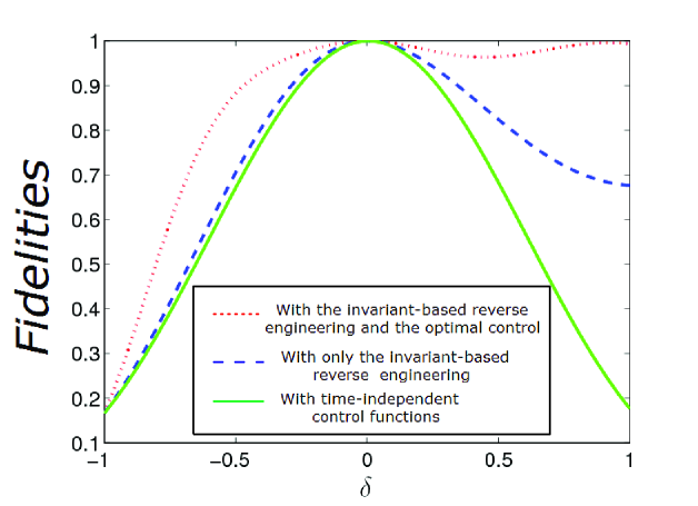
Figure 2: The fidelities of obtaining the singlet state versus $\delta$ with the invariant-based reverse engineering and the optimal control (red-dotted line), with only reverse engineering (blue-dashed line), and with the time-independent control functions (green-solid line).

Now, with the coupling strengths $g(t)$ and $J$ being settled, we now demonstrate the effect of optimal control to the generation of the singlet state via numerical simulations. Firstly, we plot the fidelity of obtaining the singlet state versus $\delta$ in Fig. 2 by the red-dotted line. As comparisons, we plot fidelities of obtaining the singlet state with another two group of control functions $g_{1}(t)$ and $g_{2}(t)$. One group is using time-independent control functions $g_{1}(t)=1.2358/T$ and $g_{2}(t)=1.2057/T$, where the fidelity of obtaining the singlet state versus $\delta$ is plotted in Fig. 2 by the blue-dashed line. The other group is using control functions given by invariant-based reverse engineering with parameters

$$\theta(t)=\frac{\pi}{4}\sin^{2}(\frac{\pi t}{2T}),\ \beta(t)=\beta(0)+[\beta(T)-\beta(0)]\sin^{4}(\frac{\pi t}{2T}),$$ (36)

which are two arbitrary functions satisfying the boundary conditions, and the fidelity of obtaining the singlet state is plotted in Fig. 2 by the green-solid line. Seen from the red-dotted line in Fig. 2, we can find that the fidelity is quite robust against systematic error of the control field $g(t)$ when it is designed by inverse engineering and optimal control. We can find in the figure that the fidelity is kept higher than 90% in a very large range $\delta\in[-0.46,1]$. However, seen from blue-dashed line, when using inverse engineering without optimal control, the fidelity is more sensitive to the systematic error of $g(t)$, where one can only obtain $F\geq 90\%$ with $\delta\in[-0.28,0.335]$. Furthermore, for time-independent control functions, the situation is much worse. According to the green-solid line in Fig. 2, the range of obtaining $F\geq 90\%$ is $\delta\in[-0.25,0.26]$, even narrower than that with only inverse engineering. Thus, optimal control help us greatly improve the robustness against the systematic error of the control fields $g(t)$.

VI Further optimization by using periodic modulation

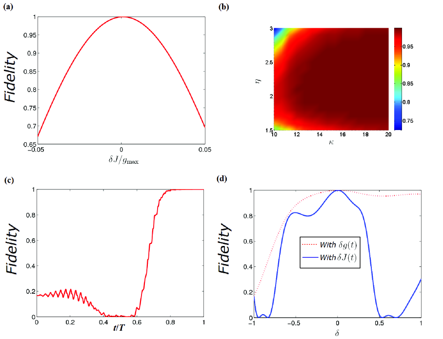
Figure 3: (a) The fidelity of obtaining the singlet state versus $\delta J/g_{\max}$ without using the periodical modulation. (b) The fidelity of obtaining the singlet state $|\Psi_{s}\rangle$ versus $\kappa$ and $\eta$. (d) The fidelity of obtaining the singlet state versus $\delta$ with the systematic errors $\delta g(t)$ (red-dotted line) and $\delta J(t)$ (blue-solid line).

In Sec. V, we have used optimal control theory to help us to weaken influence of the systematic error $\delta g(t)$. However, the systematic error of the coupling strength $J$ has not yet been considered. Since the condition $J\gg|g(t)|$ is exploited to build up the effective Hamiltonian, the systematic error of $J$ may not be considered as a perturbation in some cases. For example, when $J=300/T$, ten percent of $J$ is even larger than the maximal value of $g(t)$. This may make time-dependent perturbation theory invalid in processing the systematic error of $J$. In Fig. 3(a), we plot fidelity of obtaining the singlet state versus $\delta J/g_{\max}$ with $\delta J$ being the systematic error of $J$. We can see from Fig. 3(a) that, the fidelity decreases a lot with the increase of $\delta J$. When $\delta J=-0.05g_{\max}$ and $\delta J=0.05g_{\max}$, the fidelities are only about $67.72\%$ and $70.19\%$, respectively. To obtain fidelities higher than 90%, one should control $\delta J/g_{\max}$ in $[-0.0258,0.0278]$. This may be sometimes a strict limit for a real experiment.

According to Eq. (16), we can find that $\delta J$ breaks the resonance. When systematic error $\delta J$ appears, the faulty effective Hamiltonian should be

$$H_{e}^{\prime\prime}(t)=H_{e}(t)+\delta J(3|\phi_{1}\rangle\langle\phi_{1}|+|\phi_{2}\rangle\langle\phi_{2}|).$$ (37)

The second term of Eq. (37) leads rapid oscillations of phases when $\delta J/g_{\max}$ can not be neglected, and evolution paths given by $H_{e}(t)$ become no longer valid. Thus, to build up an evolution path insensitive to $\delta J$, we should find an alternative resonance condition independent to $J$, so that $\delta J$ may not lead significant influence to the evolution. From this point, we exploit another way, periodic modulation, to optimize the fidelity under influence of $\delta J$. Here, we consider a periodical coupling strength as  $J(t)=J_{0}\cos(\omega t)$. In the rotation frame of $R(t)=\exp(-i\int_{0}^{t}H_{s}(t^{\prime})dt^{\prime})$, the Hamiltonian of the system becomes

$$H_{R}(t)=g(t)e^{-i\eta\sin(\omega t)}[e^{3i\eta\sin(\omega t)}|\psi_{1}\rangle+|\psi_{3}\rangle+|\psi_{5}\rangle](\langle\psi_{2}|+\langle\psi_{4}|+\langle\psi_{6}|)+\mathrm{H.c.},$$ (38)

with $\eta=J_{0}/\omega$. Considering Fourier expansions with a period $\tilde{T}=2\pi/\omega$, we have

$$e^{-i\eta\sin(\omega t)}=\sum\limits_{m=-\infty}^{+\infty}\mathcal{J}_{m}(\eta)e^{-im\omega t},\ e^{2i\eta\sin(\omega t)}=\sum\limits_{m=-\infty}^{+\infty}\mathcal{J}_{m}(2\eta)e^{im\omega t},$$ (39)

with the $m$-th Bessel function $\mathcal{J}_{m}(\eta)$. By setting the control function $g(t)$ as

$$g(t)=[\bar{g}_{1}(t)\sin(\omega t)+\bar{g}_{2}(t)\sin(3\omega t)]/\sqrt{3},$$ (40)

the effective Hamiltonian $\tilde{H}_{e}(t)$ with periodic modulation can be derived as

$$\tilde{H}_{e}(t)=i\tilde{g}_{1}(t)|\phi_{1}\rangle\langle\phi_{2}|-i\tilde{g}_{2}(t)|\phi_{3}\rangle\langle\phi_{2}|+\mathrm{H.c.},$$ (41)

$$\tilde{g}_{1}(t)=\mathcal{J}_{1}(2\eta)\bar{g}_{1}(t)+\mathcal{J}_{3}(2\eta)\bar{g}_{2}(t),$$

$$\tilde{g}_{2}(t)=\sqrt{2}[\mathcal{J}_{1}(\eta)\bar{g}_{1}(t)+\mathcal{J}_{3}(\eta)\bar{g}_{2}(t)],$$

under the condition $|\bar{g}_{1}(t)|,|\bar{g}_{2}(t)|\ll\omega$. Since $\tilde{H}_{e}(t)$ has the same form as $H_{e}(t)$ shown in Eq. (17), the evolution governed by $\tilde{H}_{e}(t)$ can also be studied by invariant-based reverse engineering. Consequently, we can derive expressions of $\tilde{g}_{1}(t)$ and $\tilde{g}_{2}(t)$ in the same way. Then, one can reversely obtain $g(t)$ with

$$\bar{g}_{1}(t)=[\sqrt{2}\mathcal{J}_{3}(\eta)\tilde{g}_{1}(t)-\mathcal{J}_{3}(2\eta)\tilde{g}_{2}(t)]/\Upsilon,$$ (42)

$$\bar{g}_{2}(t)=[-\sqrt{2}\mathcal{J}_{1}(\eta)\tilde{g}_{1}(t)+\mathcal{J}_{1}(2\eta)\tilde{g}_{2}(t)]/\Upsilon,$$

$$\Upsilon=\sqrt{2}[\mathcal{J}_{1}(2\eta)\mathcal{J}_{3}(\eta)-\mathcal{J}_{3}(2\eta)\mathcal{J}_{1}(\eta)].$$

With Eqs. (41-42), let us analyze influence of the systematic errors $\delta J(t)$ and $\delta g(t)$ again. For $\delta g(t)$, it leads a faulty Hamiltonian as $\delta\tilde{H}_{e}(t)$, and this kind of error has been optimized by optimal control in Sec. V. For $\delta J$, its leads a faulty Hamiltonian as

$$H_{J}^{\prime}(t)=\delta J_{0}\cos(\omega t)(3|\phi_{1}\rangle\langle\phi_{1}|+|\phi_{2}\rangle\langle\phi_{2}|).$$ (43)

If we move to the frame of $R^{\prime}(t)=\exp(-i\int_{0}^{t}H_{J}^{\prime}(t^{\prime})dt^{\prime})$, different from the case without periodic modulation, where $\delta J$ leads rapid oscillations of phases, $\delta J(t)$ here only induces small error of the parameter $\eta$ in the effective coupling strengths $\tilde{g}_{1}(t)$ and $\tilde{g}_{2}(t)$ as $\delta\eta=\delta J_{0}/\omega$ when $\delta J_{0}\ll\omega$.

Similar result can also be obtained in the frame of $R(t)$ without using $R^{\prime}(t)$ when $\omega\gg\delta J_{0}$. Firstly, we investigate the evolution in a single period $[0,\tilde{T}]$, where the evolution operator can be approximately described as

$$\tilde{U}_{e}^{\prime}(\tilde{T},0)\simeq 1-i\int_{0}^{\tilde{T}}[H_{J}^{\prime}(t)+\tilde{H}_{e}(t)]dt=1-i\int_{0}^{\tilde{T}}\tilde{H}_{e}(t)dt\simeq\tilde{U}_{e}(\tilde{T},0),$$ (44)

with $\tilde{U}_{e}^{\prime}(\tilde{T},0)$ $(\tilde{U}_{e}(\tilde{T},0))$ being the faulty (perfect) evolution operator in time interval $[0,\tilde{T}]$, since $\delta J_{0}\tilde{T}\ll 1$. Thus, the total evolution operator (assuming $T=M\tilde{T}$, $M\in N^{+}$)

$$\tilde{U}_{e}^{\prime}(T,0) =\tilde{U}_{e}^{\prime}(T,(M-1)\tilde{T})...\tilde{U}_{e}^{\prime}(2\tilde{T},\tilde{T})\tilde{U}_{e}^{\prime}(\tilde{T},0)$$ (45)

$$\simeq\tilde{U}_{e}(T,(M-1)\tilde{T})...\tilde{U}_{e}(2\tilde{T},\tilde{T})\tilde{U}_{e}(\tilde{T},0)=\tilde{U}_{e}(\tilde{T},0),$$

is nearly perfect with $\omega\gg\delta J_{0}$. Apart from optimization to fidelity under influence of $\delta J(t)$, periodic modulation also bring some other benefits. For example, we have $R(T)=1$ $(T=M\tilde{T})$ with periodic modulation, i.e., the rotation frame of $R(t)$ coincides with the original frame at the final time. This means we do not need any additional operation to bring the singlet state in the rotation frame back to the original frame. For that without periodic modulation, although we can apply an additional operation in time interval $[T,T^{\prime}]$ with coupling strengths $J\rightarrow J^{\prime}$, $g(t)=0$ and $J^{\prime}(T^{\prime}-T)+JT=2m\pi$ ($m=0,1,2,...$) to bring the singlet state back to the original frame, more operation time is required. Thus, periodic modulation may help to save the total interaction time if entanglement generations are considered in the original frame.

To check validity of periodic modulation and select suitable parameters for $\omega$ and $J_{0}$, we plot the fidelity of obtaining the singlet state $|\Psi_{s}\rangle$ versus $\kappa=\omega T/2\pi$ and $\eta$ in Fig. 3(b). According to Fig. 3(b), the fidelity increases with the increase of $\kappa$ since the effective Hamiltonian requires the condition $|g(t)|\ll\omega$ well satisfied. But for values of $\eta$, the maximal fidelity appears about $\eta=2.3$ when $\kappa$ is fixed. We find that $\eta=2.3$ is a local maximum for $|\Upsilon|$ in Eq. (42). According to Eq. (42), a larger value for $|\Upsilon|$ produces smaller amplitude for $g(t)$. Consequently, when $\eta$ is selected for a larger $|\Upsilon|$, the condition $|g(t)|\ll\omega$ satisfy better, and one obtains higher fidelity. Thus, we select $\eta=2.3$ and $\kappa=16$ in the following discussions. The fidelity of obtaining the singlet state versus $t/T$ with periodic modulation is plotted in Fig. 3(c). Seen from Fig. 3(c), infidelity of the preparation of singlet state is only $1.377\times 10^{-4}$, while the maximal value of $J(t)$ in this case is $J_{0}=231.22/T$. Compared with the result without using periodic modulation, we can obtain higher fidelity of singlet state with smaller coupling strength $J(t)$.

Now, let us show that the generation of the singlet state is robustness against both systematic errors $\delta J(t)$ and $\delta g(t)$ with numerical simulations. Firstly, we plot fidelity of obtaining the singlet state versus $\delta$ with systematic errors $\delta g(t)$ by the red-dotted line in Fig. 3(d). Seen from Fig. 3(d), shape of the red-dotted line is similar to that in Fig. 2. The range of obtaining fidelities higher than 90% is also $\delta\in[-0.46,1]$. This is because the structures of the effective Hamiltonian and the faulty Hamiltonian leads by $\delta g(t)$ are both unchanged with periodic modulation. As a result, the parameters selected in optimal control theory in Sec. V are also applicable with periodic modulation. Accordingly, the robustness against $\delta g(t)$ is also reserved when we consider periodic modulation. On the other hand, we plot the fidelity of obtaining the singlet state versus $\delta$ with systematic errors $\delta J(t)$ by the blue-solid line in Fig. 3(d). According to the blue-solid line in Fig. 3(d), when considering the systematic error $\delta J(t)$, the fidelity is kept higher than 90% if $\delta$ is restricted in range $[-0.16,0.18]$. By substituting $J_{0}\simeq 231.22/T$, we have the $\max\limits_{0\leq t\leq T}|\delta J(t)|\leq 41.62/T$ with $\delta\in[-0.16,0.18]$. Considering $\tilde{g}_{\max}=\max\limits_{0\leq t\leq T}\{|\bar{g}_{1}(t)|,|\bar{g}_{2}(t)|\}\simeq 20.29/T$, the maximal value of $\delta J(t)$ can be almost twice as large as $\tilde{g}_{\max}$. Compared with the result in the case without periodic modulation, where one can only get fidelity higher than 90% with $\delta J/g_{\max}\in[-0.0258,0.0278]$ (or $\delta\in[-0.0017,0.0018]$), robustness against the systematic error of the coupling strength $J(t)$ is greatly improved by periodic modulation. Thus, periodic modulation make the generation of the singlet state more feasible in a real experiment.

VII Discussions

VII.1 Experimental considerations

We now make some experimental considerations about the implementation of the protocol. Firstly, we use tunable exchange interactions with strengths $J(t)$ and $g(t)$ to realize the generation of the singlet state. In practice, electron spins in quantum dot systems may be an alternative candidate for the experimental implementation of the protocol. For quantum dot systems, tunable exchange interactions can be built up between spins in two dots ZajacSci359 ; RussPRB97 ; VargasPRB100 . Before implementing experiments, the relationship between strengths of exchange interactions and gate voltages can be established by empirical formulas with some parameters being predetermined via measurements. Accordingly, the strengths can be controlled by tuning gate voltages in processes of experiments. For example, we consider the formula established in Ref. ZajacSci359 , where strength of exchange interaction can be written by a function of gate voltage $V_{M}$ as

$$J(V_{M})=\mathcal{C}\frac{V_{M_{0}}-V_{M}}{(V_{M}-V_{M_{1}})^{2}}\exp(-\sqrt{\frac{|V_{M}-V_{M_{0}}|}{V_{on}}}),$$ (46)

In Eq. (46), $V_{M_{1}}$ is the voltage at which the tunneling barrier height is zero, $V_{M_{0}}$ is the voltage at which the barrier height equals the electron energy, and $V_{on}$ is the voltage scale of the sub-exponential increase of $J$ with $V_{M}$, and $\mathcal{C}$ is an overall scale factor. Form Eq. (46), it is possible to tune the coupling strengths $J(t)$ and $g(t)$ by converting the time dependence of the coupling strengths to that of the gate voltages. In addition, periodic modulation can be realized by tuning gate voltage around $V_{M_{0}}$.

In the generation of the singlet state without periodic modulation, considering an available coupling strength $J=20$MHz ZajacSci359 ; RussPRB97 ; VargasPRB100 , the total interaction time is $T=15\mu$s, according to the selection $J=300/T$. The interaction time is much less than the coherence time of spin qubits in quantum dots XZLRMP85 . Moreover, the tuning frequencies of the components $g_{1}(t)$ and $g_{2}(t)$ of $g(t)$ is less than $2J=40$MHz, which are also feasible with fast gate voltage tuning of quantum dots ZajacSci359 .

In addition, for the generation of the singlet state with periodic modulation, we consider an available intensity for the coupling strength $J(t)$ as $J_{0}=20$MHz ZajacSci359 ; RussPRB97 ; VargasPRB100 . The total interaction time is $T=11.56\mu$s given by $J_{0}=231.22/T$. Moreover, the tuning frequency of $J(t)$ is $\omega=8.7$MHz, and the tuning frequency of $g(t)$ is less than $3\omega=26.1$MHz according to Eq. (40). The tuning frequencies of $g(t)$ and $J(t)$ are also feasible with fast gate voltage tuning in quantum dot systems ZajacSci359 . Thus, the tuning of strength is feasible in the protocol by using the technology shown in Ref. ZajacSci359 .

On the other hand, the systematic errors of coupling strengths discussed in Sec. V and Sec. VI are also proper to describe the influence of charge noise in quantum dot systems. Previous protocols RussPRB97 ; VargasPRB100 have shown that charge noise is a main disturbing factor leading fluctuations of electric potentials near dots, and results in deviations of coupling strengths as $J(t)\rightarrow J(t)+\delta J(t)$ and $g(t)\rightarrow g(t)+\delta g(t)$ in the first order approximation. Typically, the noise level is about 1% of the original coupling strength VargasPRB100 . With optimizations in the protocol, fidelity of obtaining the logical qubit singlet state can be higher than 0.998.

Apart from electron spins in quantum dot system, nuclear spins in NMR systems may also be considered to implement the protocol. Recent experimental protocols JYPRA99 ; PXPRL103 have shown tunable exchange interactions can be effectively realized via NMR pulsing techniques PXPRL103 ; VandersypenRMP76 . With the help of external magnetic field sequences and natural $\sigma_{z}\otimes\sigma_{z}$ couplings of nuclear spins, exchange interactions in different directions with different strengths can be simulated. Furthermore, the undesired interactions can be switched off via the refocusing technique shown in Ref. VandersypenRMP76 . Therefore, any operations in a short time interval can be equivalently produced by the NMR pulsing techniques, and the total operation can be composed through Trotter’s formula SuzukiPJASB69 . The discussions about the systematic errors of coupling strengths can also applied to reduce influence of imperfect refocusing and deviations of coupling strengths of nuclear spins due to imperfect calibration.

VII.2 Performance in decoherence environment

When a spin system is not well isolated from environment, decoherence may disturb the unitary evolution of the spin systems. Ref. BayatNJP17 have shown that the dephasing due to random energy fluctuations induced on qubit levels by random magnetic and electric fields in the environment, is one of the challenges in real experiments when the number of spins increases. Under influence of dephasing, evolution of the system is governed by the master equation BayatNJP17

$$\dot{\rho}(t)=i[\rho(t),H(t)]+\sum\limits_{j=1}^{3}\sum\limits_{\iota=1}^{2}\gamma[\sigma_{z}^{(q_{j_{\iota}})}\rho(t)\sigma_{z}^{(q_{j_{\iota}})}-\rho(t)],$$ (47)

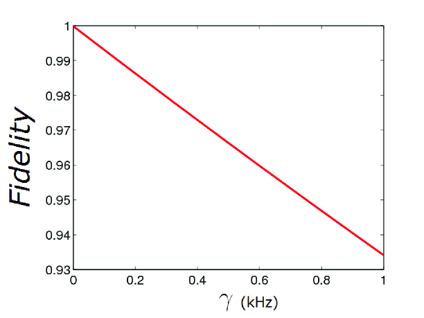
Figure 4: Fidelities of obtaining the singlet state versus dephasing rate $\gamma$.

where $\gamma$ is the dephasing rate. Based on Eq. (47), the fidelity of obtaining the singlet state versus dephasing rate $\gamma$ is plotted in Fig. 4. Considering reported coherence time of electron spins in quantum dots about ms-s XZLRMP85 , the range of $\gamma$-axis is set from 0 to 1kHz. As shown by Fig. 4, the fidelity is 0.9931 when $\gamma=0.1$kHz. The protocol can still perform well when the coherence time is about 10ms. Moreover, for $\gamma=1$kHz, the fidelity is still 0.9342. Therefore, even when we consider a shorter coherence time about 1 ms, the protocol can still produce fidelities higher than 0.9.

VIII Conclusion

In conclusion, we have proposed a protocol to realize the generation of singlet states of three logical qubits constructed by pairs of spins. The protocol contains comprehensive consideration of control Hamiltonian, invariant-based reverse engineering, optimal control and periodic modulation. Firstly, single-qubit and multi-qubit interactions of logical qubits were analyzed, and the effective Hamiltonian was built up. Secondly, invariant-based reverse engineering was successfully used in studying the evolution governed by the effective Hamiltonian, and an evolution path was established for the generation of the target state. Thirdly, optimal control theory was exploited in selections of control parameters. We showed that the entanglement generation is robust against the systematic error of coupling strength $g(t)$. Fourthly, to further improve robustness of the protocol, we applied periodic modulation to coupling strengths $g(t)$ and $J(t)$, and derived an effective Hamiltonian with similar structure as that in the case without periodic modulation. In this way, the preparation of the singlet state benefited from invariant-based reverse engineering, optimal control and periodic modulation simultaneously, and became robust against systematic errors of coupling strengths $g(t)$ and $J(t)$. As the protocol can produce acceptable fidelity in a relative wide range of systematic errors, and spin systems also possess nice inherent controllability ZajacSci359 ; RussPRB97 ; PXPRL103 ; VargasPRB100 ; VandersypenRMP76 to modulate time-dependent couplings in tolerable error ranges, the protocol may be feasible in experiments. We hope the protocol can be helpful to robust generations of logical qubit singlet state with spin systems.

Appendix: Initialization of logical qubits

Since quantum information of logical qubit is encoded in Bell-state basis $|0\rangle$, $|1\rangle$ and $|2\rangle$, and the initial state we considered in the generation of singlet state is $|012\rangle$, discussions about initialization of logical qubits may be useful. Here, Hamiltonian for initialization of the logical qubit $q_{j}$ is considered as

$$H_{i}(t) =\frac{B_{x}(t)}{2}[\sigma_{x}^{(q_{j_{1}})}+\sigma_{x}^{(q_{j_{1}})}]+\frac{B_{z}(t)}{2}[\sigma_{z}^{(q_{j_{1}})}+\sigma_{z}^{(q_{j_{1}})}]$$ (48)

$$+\frac{J_{yj}}{4}\sigma_{y}^{(q_{j_{1}})}\otimes\sigma_{y}^{(q_{j_{2}})},$$

where $B_{x}(t)$ and $B_{z}(t)$ are magnetic fields along $x$-axis and $z$-axis. In the Bell-state basis $\{|0\rangle_{j},|1\rangle_{j},|2\rangle_{j},|3\rangle_{j}\}$, $H_{i}(t)$ can be described as

$$H_{in}(t)=H_{inB}(t)+H_{inJ},$$ (49)

$$H_{inB}(t)=[B_{x}(t)|0\rangle\langle 1|+B_{z}(t)|0\rangle\langle 2|]/2+\mathrm{H.c.},$$

$$H_{inJ}=\frac{J_{yj}}{4}(|1\rangle_{j}\langle 1|+|2\rangle_{j}\langle 2|-|0\rangle_{j}\langle 0|-|3\rangle_{j}\langle 3|).$$

In the rotation frame of $R_{in}(t)=\exp(-iH_{inJ}t)$, the Hamiltonian becomes

$$H_{inR}(t)=e^{-iJ_{yj}t/2}[B_{x}(t)|0\rangle\langle 1|+B_{z}(t)|0\rangle\langle 2|]/2+\mathrm{H.c.}$$ (50)

If we set the variations of magnetic fields as

$$B_{x}(t)=2\bar{B}_{x}(t)\sin(J_{yj}t),\ B_{z}(t)=-2\bar{B}_{z}(t)\sin(J_{yj}t),\$$ (51)

we can obtain an effective Hamiltonian as

$$H_{ine}(t)=i\bar{B}_{x}(t)|1\rangle\langle 0|-i\bar{B}_{z}(t)|2\rangle\langle 0|+\mathrm{H.c.}$$ (52)

Noticing that $H_{ine}(t)$ possesses the same structure as $H_{e}(t)$ in Eq. (17) with $\bar{B}_{x}(t)\rightarrow g_{1}(t)$ and $\bar{B}_{z}(t)\rightarrow g_{2}(t)$, the invariant $I(t)$ in form of Eq. (22) can still be applied to $H_{ine}(t)$ by changing basis from $\{|\phi_{1}\rangle,|\phi_{2}\rangle,|\phi_{3}\rangle\}$ to the basis $\{|1\rangle,|0\rangle,|2\rangle\}$, and the eigenstate $|\Phi_{0}(t)\rangle$ of $I(t)$ can still be used as an evolution path for initialization. Assuming that the initial state is the product state $|\downarrow\downarrow\rangle_{q_{j1}q_{j2}}=\frac{1}{\sqrt{2}}(|0\rangle_{j}-|2\rangle_{j})$, the system can evolves from $|\downarrow\downarrow\rangle_{q_{j1}q_{j2}}$ to $|0\rangle_{j}$ ($|1\rangle_{j}$, $|2\rangle_{j}$) when the boundary condition is set as $\{\theta(0),\beta(0)\}=\{-3\pi/4,0\}$ and $\{\theta(T),\beta(T)\}=\{-\pi/2,\mathrm{arbitrary\ angle}\}$ ($\{\theta(T),\beta(T)\}=\{0,\pi/2\}$, $\{\theta(T),\beta(T)\}=\{0,0\}$).

Moreover, initialization of logical qubits can also optimized by optimal control and periodic modulation. For example, to use periodic modulation, one can set

$$J_{yj}(t)=2J_{y0}\cos(\omega t),$$ (53)

$$B_{x}(t)=2\tilde{B}_{x}(t)\sin(\omega t)/\mathcal{J}_{1}(J_{y0}/\omega),$$

$$B_{z}(t)=-2\tilde{B}_{z}(t)\sin(\omega t)/\mathcal{J}_{1}(J_{y0}/\omega).$$

Then, by moving into the rotation frame of $\tilde{R}_{in}(t)=\exp{-i\int_{0}^{t}H_{inJ}(t^{\prime})dt^{\prime}}$, an effective Hamiltonian can be derived as

$$\tilde{H}_{ine}(t)=i\tilde{B}_{x}(t)|1\rangle\langle 0|-i\tilde{B}_{z}(t)|2\rangle\langle 0|+\mathrm{H.c.}$$ (54)

Subsequently, evolutions governed by effective Hamiltonian $\tilde{H}_{ine}(t)$ can be further studied with invariant-based reverse engineering and optimal control.

References

- (1) J. S. Bell, Physics 1965, 1, 195.
- (2) D. M. Greenberger, M. A. Horne, A. Shimony, A. Zeilinger, Am. J. Phys. 1990, 58, 1131.
- (3) W. Dür, G. Vidal, J. I. Cirac, Phys. Rev. A 2000, 62, 062314.
- (4) A. Cabello, Phys. Rev. A 2002, 65, 032108.
- (5) C. H. Bennett, D. P. DiVincenzo, Nature 2000, 404, 247.
- (6) H. E. Türeci, J. M. Taylor, A. Imamoglu, Phys. Rev. B 2007, 75, 235313.
- (7) G. W. Lin, M. Y. Ye, L. B. Chen, Q. H. Du, X. M. Lin, Phys. Rev. A 2007, 76, 014308.
- (8) W. A. Li, G. Y. Huang, Phys. Rev. A 2011, 83, 022322.
- (9) X. Q. Shao, T. Y. Zheng, C. H. Oh, S. Zhang, Phys. Rev. A 2014, 89, 012319.
- (10) C. Song, S. L. Su, J. L. Wu, D. Y. Wang, X. Ji, S. Zhang, Phys. Rev. A 2016, 93, 062321.
- (11) F. Fröwis, W. Dür, Phys. Rev. Lett. 2011, 106, 110402.
- (12) W. J. Munro, A. M. Stephens, S. J. Devitt, K. A. Harrison, K. Nemoto, Nat. Photon. 2012, 6, 777.
- (13) F. Fröwis, W. Dür, Phys. Rev. A 2012, 85, 052329.
- (14) L. Zhou, Y. B. Sheng, Phys. Rev. A 2015, 92, 042314.
- (15) D. Ran, W. J. Shan, Z. C. Shi, Z. B. Yang, J. Song, and Y. Xia, Phys. Rev. A 2020, 102, 022603.
- (16) Y. H. Chen, W. Qin, X. Wang, A. Miranowicz, F. Nori, arXiv:2008.04078.
- (17) D. Kaszlikowski, P. Gnacinski, M. Zukowski, W. Miklaszewski, A. Zeilinger, Phys. Rev. Lett. 2000, 85, 4418.
- (18) M. Bourennane, A. Karlsson, G. Björk, Phys. Rev. A 2001, 64, 012306.
- (19) D. Bruß, C. Macchiavello, Phys. Rev. Lett. 2002, 88, 127901.
- (20) N. J. Cerf, M. Bourennane, A. Karlsson, N. Gisin, Phys. Rev. Lett. 2002, 88, 127902.
- (21) A. Cabello, Phys. Rev. Lett. 2002, 89, 100402.
- (22) N. D. Mermin, Phys. Rev. D 1980, 22, 356.
- (23) A. Cabello, J. Mod. Opt. 2003, 50, 1049.
- (24) H. Sun, P. Xu, H. Pu, W. Zhang, Phys. Rev. A 2017, 95, 063624.
- (25) X. Q. Shao, T. Y. Zheng, S. Zhang, Phys. Rev. A 2012 85, 042308.
- (26) X. Chen, H. Xie, G. W. Lin, X. Shang, M. Y. Ye, X. M. Lin, Phys. Rev. A 2017, 96, 042308.
- (27) X. Q. Shao, Z. H. Wang, H. D. Liu, X. X. Yi, Phys. Rev. A 2016 94, 032307.
- (28) X. Chen, G. W. Lin, H. Xie, X. Shang, M. Y. Ye, X. M. Lin, Phys. Rev. A 2018, 98, 042335.
- (29) X. Q. Shao, H. F. Wang, L. Chen, S. Zhang, Y. F. Zhao, K. H. Yeon, New J. Phys. 2010, 12, 023040.
- (30) M. K. Henry, C. Ramanathan, J. S. Hodges, C. A. Ryan, M. J. Ditty, R. Laflamme, D. G. Cory, Phys. Rev. Lett. 2007, 99, 220501.
- (31) B. Shaw, M. M. Wilde, O. Oreshkov, I. Kremsky, D. A. Lidar, Phys. Rev. A 2008, 78, 012337.
- (32) J. Zhang, R. Laflamme, D. Suter, Phys. Rev. Lett. 2012, 109, 100503.
- (33) E. Kapit, Phys. Rev. Lett. 2018, 120, 050503.
- (34) Z. D. Walton, A. F. Abouraddy, A. V. Sergienko, B. E. A. Saleh, M. C. Teich, Phys. Rev. Lett. 2003, 91, 087901.
- (35) Y. B. Sheng, L. Zhou, Sci. Rep. 2015, 5, 13453.
- (36) L. Zhou, Y. B. Sheng, Sci. Rep. 2016, 6, 28813.
- (37) L. Hu, Y. Ma, W. Cai, X. Mu, Y. Xu, W. Wang, Y. Wu, H. Wang, Y. P. Song, C. L. Zou, S. M. Girvin, L. M. Duan, L. Sun, Nat. Phys. 2019, 15, 503.
- (38) C. Qu, L. Zhou, Y. B. Sheng, Quantum Inf. Process. 2015, 14, 4131.
- (39) X. Wu, L. Zhou, W. Zhong, Y. B. Sheng, Quantum Inf Process. 2018, 17, 255.
- (40) L. Zhou, Y. B. Sheng, Sci. Rep. 2016, 6, 20901.
- (41) F. Kesting, F. Fröwis, W. Dür, Phys. Rev. A 2013, 88, 042305.
- (42) H. Lu, L. K. Chen, C. Liu, P. Xu, X. C. Yao, L. Li, N. L. Liu, B. Zhao, Y. A. Chen, J. W. Pan, Nat. Photon. 2014, 8, 364.
- (43) Z. L. Xiang, S. Ashhab, J. Q. You, F. Nori, Rev. Mod. Phys. 2013, 85, 623.
- (44) K. Paul, A. K. Sarma, Phys. Rev. A 2016, 94, 052303.
- (45) D. Stefanatos, E. Paspalakis, Phys. Rev. A 2019, 99, 022327.
- (46) X. T. Yu, Q. Zhang, Y. Ban, X. Chen, Phys. Rev. A 2018, 97, 062317.
- (47) L. Jin, Z. Song, Phys. Rev. A 2009, 79, 042341.
- (48) J. Chen, H. Zhou, C. Duan, X. Peng, Phys. Rev. A 2017, 95, 032340.
- (49) Y. Ji, J. Bian, X. Chen, J. Li, X. Nie, H. Zhou, X. Peng, Phys. Rev. A 2019, 99, 032323.
- (50) Y. H. Kang, Z. C. Shi, B. H. Huang, J. Song, Y. Xia, Phys. Rev. A 2019, 100, 012332.
- (51) X. Chen, J. G. Muga, Phys. Rev. A 2012, 86, 033405.
- (52) F. Impens, D. Guéry-Odelin, Phys. Rev. A 2017, 96, 043609.
- (53) D. Guéry-Odelin, A. Ruschhaupt, A. Kiely, E. Torrontegui, S. Martínez-Garaot, J. G. Muga, Rev. Mod. Phys. 2019, 91, 045001.
- (54) S. Ibáñez, X. Chen, J. G. Muga, Phys. Rev. A 2013, 87, 043402.
- (55) E. Torrontegui, S. Martínez-Garaot, J. G. Muga, Phys. Rev. A 2014, 89, 043408.
- (56) Y. H. Kang, Z. C. Shi, B. H. Huang, J. Song, Y. Xia, Phys. Rev. A 2020, 101, 032322.
- (57) A. Ruschhaupt, X. Chen, D. Alonso, J. G. Muga, New J. Phys. 2012, 14, 093040.
- (58) D. Daems, A. Ruschhaupt, D. Sugny, S. Guérin, Phys. Rev. Lett. 2013, 111, 050404.
- (59) L. Van Damme, Q. Ansel, S. J. Glaser, D. Sugny, Phys. Rev. A 2017, 95, 063403.
- (60) L. Van-Damme, D. Schraft, G. T. Genov, D. Sugny, T. Halfmann, S. Guérin, Phys. Rev. A 2017, 96, 022309.
- (61) X. J. Lu, X. Chen, A. Ruschhaupt, D. Alonso, S. Guérin, J. G. Muga, Phys. Rev. A 2013, 88, 033406.
- (62) Y. H. Kang, Z. C. Shi, J. Song, Y. Xia, Phys. Rev. A 2020, 102, 022617.
- (63) H. R. Lewis, W. B. Riesenfeld, J. Math. Phys. 1969, 10, 1458.
- (64) D. M. Zajac, A. J. Sigillito, M. Russ, F. Borjans, J. M. Taylor, G. Burkard, J. R. Petta, Science 2018, 359, 439.
- (65) M. Russ, D. M. Zajac, A. J. Sigillito, F. Borjans, J. M. Taylor, J. R. Petta, G. Burkard, Phys. Rev. B 2018, 97, 085421.
- (66) F. A. Calderon-Vargas, G. S. Barron, X. H. Deng, A. J. Sigillito, E. Barnes, S. E. Economou, Phys. Rev. B 2019, 100, 035304.
- (67) X. Peng, J. Zhang, J. Du, D. Suter, Phys. Rev. Lett. 2009, 103, 140501.
- (68) L. M. K. Vandersypen, I. L. Chuang, Rev. Mod. Phys. 2005, 76, 1037.
- (69) M. Suzuki, Proc. Jpn. Acad. Ser. B 1993, 69, 161.
- (70) A. Bayat, Y. Omar, New J. Phys. 2015, 17, 103041.