Discovery of a $\sim$30-Year-Duration Post-Nova Pulsating Supersoft Source in the Large Magellanic Cloud

Abstract

Supersoft X-ray sources (SSS) have been identified as white dwarfs accreting from binary companions and undergoing nuclear-burning of the accreted material on their surface. Although expected to be a relatively numerous population from both binary evolution models and their identification as Type Ia supernova progenitor candidates, given the very soft spectrum of SSSs relatively few are known. Here we report on the X-ray and optical properties of 1RXS J050526.3-684628, a previously unidentified accreting nuclear-burning white dwarf located in the Large Magellanic Cloud (LMC). XMM-Newton observations enabled us to study its X-ray spectrum and measure for the first time short period oscillations of $\sim$170 s. By analysing newly obtained X-ray data by eROSITA, together with Swift observations and archival ROSAT data, we have followed its long-term evolution over the last 3 decades. We identify 1RXS J050526.3-684628 as a slowly-evolving post-nova SSS undergoing residual surface nuclear-burning, which finally reached its peak in 2013 and is now declining. Though long expected on theoretical grounds, such long-lived residual-burning objects had not yet been found. By comparison with existing models, we find that the effective temperature and luminosity evolution are consistent with a $\sim$0.7 $M_{\odot}$ carbon-oxygen white dwarf accreting $\sim$10${}^{-9}\leavevmode\nobreak\ \rm{M}_{\odot}$/yr. Our results suggest there may be many more undiscovered SSSs and “missed” novae awaiting dedicated deep X-ray searches in the LMC and elsewhere.

1 Introduction

Super-soft X-ray sources (SSSs) are defined by their approximate black-body spectra with temperatures and luminosities of 20-100 eV and $\geq 10^{35}$ erg s^-1, respectively (Greiner, 1996). Many SSS are now understood to be binary systems wherein a white dwarf (WD) undergoes surface nuclear-burning of matter accreted from a companion star (Kahabka & van den Heuvel, 1997). These systems may play a vital role in the origin of i-process elements (Denissenkov et al., 2017), provide a unique probe of the warm interstellar medium (Woods & Gilfanov, 2016), and are an essential benchmark in understanding the evolution of interacting binaries (Chen et al., 2014, 2015). Perhaps most famously, if an accreting WD can grow to reach the Chandrasekhar mass limit ($\approx 1.4M_{\odot}$), it may explode as a type Ia supernova.Although the total contribution of such objects to the observed type Ia rate remains uncertain (see review Maoz et al., 2014), recent abundance measurements suggest a significant fraction of SNe Ia must originate in near-Chandrasekhar mass explosions (Hitomi Collaboration et al., 2017).

The Magellanic Clouds harbour a well studied population of SSS (Greiner, 1996). Their moderate and well known distances, as well as the low Galactic foreground absorption, make SSSs ideal targets for examining their bolometric luminosities and spectral properties. Here, we provide the first identification of 1RXS J050526.3-684628 (hereafter J050526) as a very long-lived post-nova SSS based on XMM-Newton observations carried out on February 09, 2013 (obsid: 0693450201), and on October 19, 2017 (obsid: 0803460101). Originally detected as a soft X-ray source in the LMC during the ROSAT all-sky survey (Voges et al., 1999), J050526 has remained uncharacterized until now, likely due to the low statistics in the previously available data. In the following, we report the X-ray spectral and temporal properties of the SSS system observed by XMM-Newton, which confirm the nature of this system as being consistent with an accreting white dwarf (WD) undergoing residual nuclear-burning and short-period pulsations. We also identify a possible optical counterpart from observations made by the Optical Gravitational Lensing Experiment (OGLE).

2 Data Analysis

XMM-Newton data were analysed by using the Data Analysis software SAS, version 17.0.0 and most recent calibration files. To search for background flares, we defined a background threshold of 8 and 2.5 counts ks^-1 arcmin^-2 for the EPIC-pn and EPIC-MOS detectors, respectively. Event extraction was performed using the SAS task evselect, with filtering flags (#XMMEA_EP && PATTERN<=4 for pn and #XMMEA_EM && PATTERN<=12 for MOS). SAS tasks rmfgen and arfgen were used to create the redistribution matrix and ancillary file. Finally, we performed barycentric corrections to the event arrival times.

The 2013 XMM-Newton (hereafter XMM13) observation (40 ks starting on MJD 56332.5) was affected by major background flares, thus only the first $\sim$30 ks were used for our analysis. Additionally, J050526 was projected in a CCD gap in the EPIC-pn detector ($\sim$80% of counts were lost). For the 2017 (hereafter XMM17) observation, XMM-Newton observed J050526 for 55ks (MJD 58045.2) while data were not affected by background flares.

The source detection was performed simultaneously on all the images using the SAS task edetect_chain. To account for the systematic uncertainties we performed boresight corrections based on the source position of known X-ray sources in the field of XMM-Newton. The X-ray positions were cross-corrected with those of known AGN (Kozłowski et al., 2013), and a boresight correction was computed as the median of the astrometric offsets. This resulted in a localization of J050526 at $\alpha_{\text{J2000}}=05^{\text{h}}05^{\text{m}}21\aas@@fstack{s}{}67$ and $\delta_{\text{J2000}}=-68^{\circ}45^{\prime}38\aas@@fstack{\prime\prime}0$ (0.03″, $1\sigma$ statistical uncertainty). However, the positional error is dominated by a systematic uncertainty of $\sim$0.5″ (see Sturm et al., 2013).

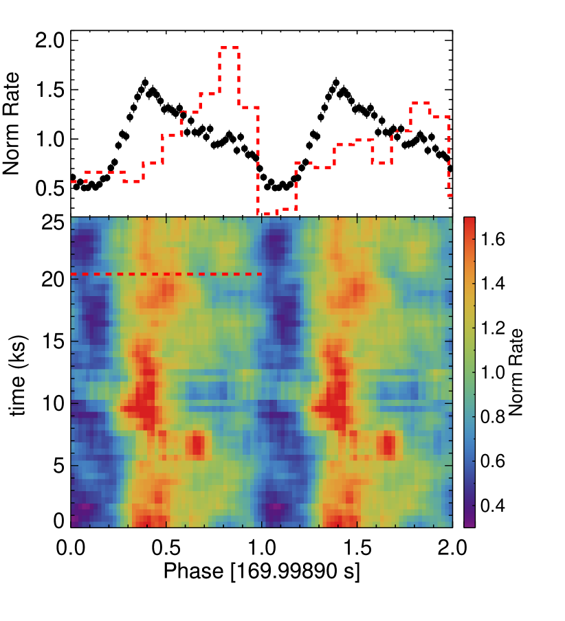
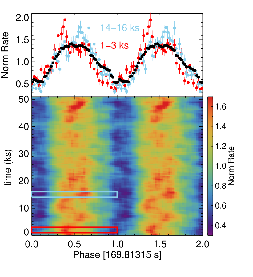
Figure 1: Time-averaged pulse profile (black points in upper panels) and dynamical pulse profiles (i.e. heat maps in lower panels) of J050526 for the 2013 (left) and 2017 (right) XMM-Newton data. In the heat-map there is evidence for a change in the pulse morphology within each observation. To better demonstrate this variability we created pulse profiles from short intervals. For XMM13 we plot two consecutive pulses on top of the time-averaged profile (dashed red line in left panel). For the XMM17 data, we created pulse profiles using 2 ks intervals and over-plotted them over the average profile. Extraction regions for the 2 pulse profiles are marked with coloured boxes on the heat map.

2.1 Timing properties

We searched for a periodic signal in the barycentric corrected XMM-Newton/EPIC events (merged event lists from the three detectors). We limited our search to events with detector energies 0.2-1.5 keV. We used epoch folding implemented through HENdrics command-line scripts (Huppenkothen et al., 2019). A period of $\sim$170 s was detected in all data. To estimate period uncertainties we followed Tsygankov et al. (2020); Vasilopoulos et al. (2020). We first calculated time of arrivals of individual pulses and then used a Bayesian approach of linear regression to fit them (Kelly, 2007). For XMM13 we found a period $P$ of 170.00$\pm$0.03 s (i.e. $\nu=0.0058824$ Hz), while for XMM17 we found $P=169.813\pm 0.014$ s (i.e. $\nu=0.0058888$ Hz). This suggests a period derivative of $\dot{P}=-1.26(20)\times 10^{-9}s/s$ (i.e. $\dot{\nu}=4.35\times 10^{-14}$ Hz/s).

We used the timing solution to create average and dynamical (i.e. heat maps) pulse profiles for the two XMM-Newton observations (see Fig. 1). The pulse profiles were created by using all XMM-Newton/EPIC events within the 0.2-1.5 keV energy band, which resulted in 25k and 100k counts from observations XMM13 and XMM17 respectively. The time-averaged pulse profiles are single peaked, however, the dynamical pulse profiles revealed some variability. Specifically, the peak of the pulse modulates between phase 0.4 and 0.7 (see XMM17 pulses in Fig. 1). By visually inspecting the light-curve we identified intervals where the profile became double-peaked with a secondary peak at phase 0.8-0.9, this is evident in two consecutive pulses around $\sim$20 ks into the XMM13 observation (see left panel in Fig. 1).

2.2 Spectral properties

All spectra were regrouped to have at least 1 count per bin. Spectral modeling was performed in XSPEC v12.10.1f (Arnaud, 1996), using C-statistics. The continuum of SSS spectra can be modeled by either an empirical black-body (BB) model, or by a non-local thermodynamic equilibrium model (NLTE) that provides a more physical description of the WD atmosphere. Both have been successfully used with CCD-quality spectra, where due to the lack of high spectral resolution not all WD atmospheric lines and absorption edges can be resolved (e.g. Greiner et al., 1994; Ebisawa et al., 2001, 2010; Ness et al., 2013). We used publicly available NLTE models for $\log{g}=9$ (in cgs units) and pure Hydrogen atmospheres (Werner & Dreizler, 1999; Rauch & Deetjen, 2003). In the source spectra there is also a high energy tail present, that can be adequately fitted by a power-law (PL) component. From inspection of the X-ray images the hard emission is consistent with a point source and thus is intrinsic to the system. The hard X-ray emission in SSS has been proposed to be due to shocks within the nova ejecta (see case for V1974 Cyg Krautter et al., 1996). To account for the photo-electric absorption we used tbabs in xspec with Solar abundances set according to Wilms et al. (2000) and atomic cross sections from Verner et al. (1996). We used two absorption components to account for the Galactic and the intrinsic absorption of the LMC and the source (e.g. Vasilopoulos et al., 2013; Vasilopoulos et al., 2014; Haberl et al., 2017). We fixed the Galactic column density to the value of $6.98\times 10^{20}$ cm^-2 (Dickey & Lockman, 1990). For the LMC component, elemental abundances were fixed at 0.49 of the solar values (Rolleston et al., 2002), and the column density was set as free fit parameter.

For the XMM2013 data we fitted the model to spectra obtained by all detectors (0.2-10.0 keV band), this was necessary as the source was positioned at the CCD gap of the EPIC-pn detector. For the 2017 fit, we only used the spectra obtained by EPIC-pn (0.2-10.0 keV band), because of the better calibration at lower energies. Uncertainties were estimated by a Markov chain Monte Carlo approach and the Goodman-Weare algorithm through xspec (Confidence level of 2.706 $\sigma$). For the 2013 data the normalization between the EPIC-mos and pn spectra was different by $\sim$20%, thus we included this uncertainty in the errors of the reported fluxes. The parameters of the best fit are presented in table 1 while the spectral fits are shown in Fig. 2.

Comparing the BB and NLTE models, the BB shows a better fit, however, this might be expected as NLTE models have been reported to insufficiently model some absorption edges (Ebisawa et al., 2010). Comparing the 2013 and 2017 data the flux (and luminosity) of the system has dropped by a factor of $\sim$2. The emission peak of either spectral component is below the lower limit of the observed spectra. Thus, for either model the fitting is affected by our choice of the spectral range. We used as a lower limit the 0.2 keV range as it is commonly used for SSS systems in the literature, but we note that fitting the data in the 0.3-10.0 keV range generally results in similar spectral shape but larger absorption and larger bolometric $L_{x}$ (factor of 2-4). This could be important when comparing with other systems, where the spectral analysis was performed in different energy bands.

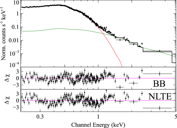
Figure 2: Left panel: 2013 XMM-Newton spectrum of J050526. In the upper panel we plot the detector spectra from EPIC-pn (black) and EPIC-mos cameras (red and cyan points). The best fit model (black steps) composed from NLTE (red) and power-law (green) components are also plotted. The lower two panels show the residuals for the models presented in table 1. Right panels: same as left but for the XMM13 data and using only the EPIC-pn detector.

Table 1: Best-fit parameters of spectral models

[b] XMM - 2013 XMM - 2017 Component Parameters BB model NLTE model BB model NLTE model Units $N_{\rm{H}}$ LMC^(a) 2.0${}^{+0.7}_{-0.7}$ 6.7${}^{+0.7}_{-0.8}$ 2.2${}^{+0.5}_{-0.4}$ 6.9${}^{+0.6}_{-0.5}$ $10^{20}$cm^-2 Bbody k${\rm T_{BB}}$ 82.2${}^{+1.4}_{-1.1}$ - 78.5${}^{+1.1}_{-1.1}$ - eV $R_{BB}$ ^(b) 1060${}^{+80}_{-80}$ - 830${}^{+50}_{-50}$ - km NLTE k${\rm T_{WD}}$ - 360${}^{+34}_{-15}$ - 328${}^{+10}_{-7}$ $10^{3}$ Kelvin $R_{WD}$ ^(c) - 14700$\pm$2900 - 13400$\pm$1200 km PL $\Gamma$ 1.7${}^{+0.6}_{-0.5}$ 0.3${}^{+0.6}_{-0.8}$ 2.5${}^{+0.5}_{-0.4}$ 1.2${}^{+0.3}_{-0.3}$ - Norm^(d) 5.8${}^{+1.6}_{-0.9}$ 6.5${}^{+2.7}_{-2.6}$ 5.6${}^{+1.8}_{-1.0}$ 4.2${}^{+0.7}_{-0.5}$ $10^{34}$ erg s^-1 $C_{\rm stat}/DOF$ 629.2/433 761.5/433 294.8/185 355.9/185 $F_{X,BB}$ (0.2-2.0) 4.1$\pm$0.4 4.0$\pm$0.4 2.06$\pm$0.1 2.07$\pm$0.1 $10^{-12}$ erg cm^-2 s^-1 $L_{X,BB/WD}$ (0.2-1.0)^(e) 4.8${}^{+0.8}_{-0.7}$ 11.2${}^{+2.3}_{-1.2}$ 2.4${}^{+0.1}_{-0.2}$ 6.0${}^{+0.4}_{-0.5}$ $10^{36}$ erg s^-1 $L_{X,WD}$ Bolom.^(f) 6.6${}^{+0.5}_{-0.4}$ 25${}^{+4}_{-3}$ 3.4${}^{+0.2}_{-0.3}$ 14.7${}^{+1.9}_{-1.6}$ $10^{36}$ erg s^{-1 (a)} Column density of the absorption component with LMC abundances, column density of Galactic absorption was fixed to 6.98$\times 10^{20}$cm^-2 (see text for details). ^(b) BB radius was estimated from the normalization of the model, assuming a distance of 50 kpc. ^(c) The size of the WD can be estimated assuming $L_{\rm X}=4\pi R_{WD}\sigma{T_{WD}^{4}}$. ^(d) Absorption corrected luminosity of the PL component in the 0.3-10.0 keV band. ^(e) Absorption corrected luminosity of the BB/NLTE component in the 0.2-1.0 keV band. ^(f) Bolometric $L_{\rm X}$ of the BB/NLTE component.

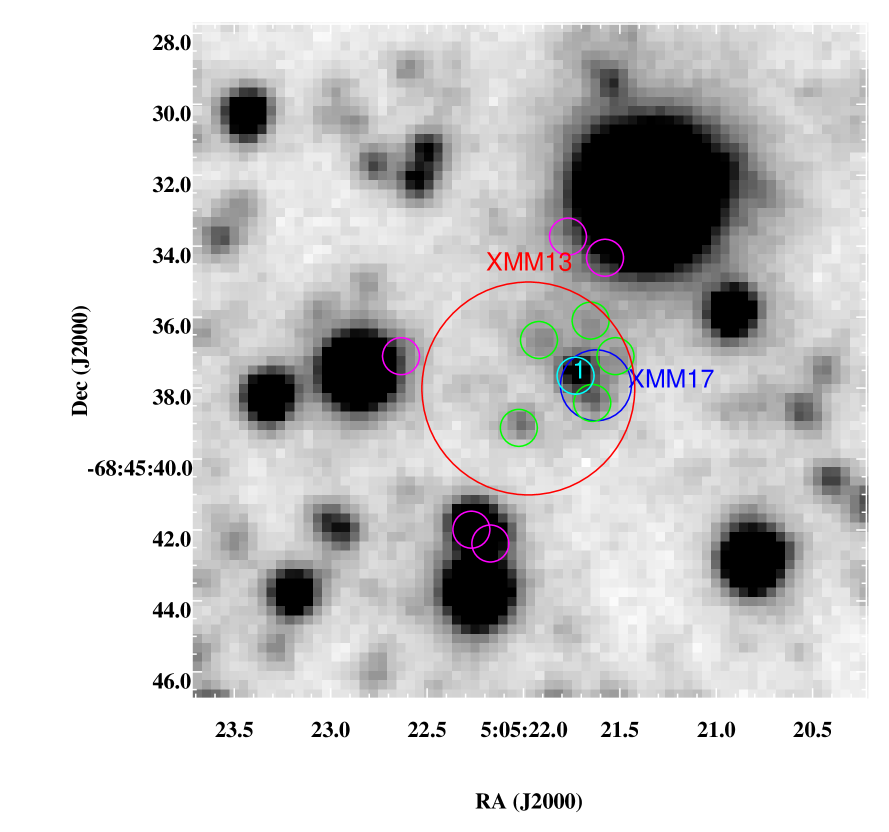
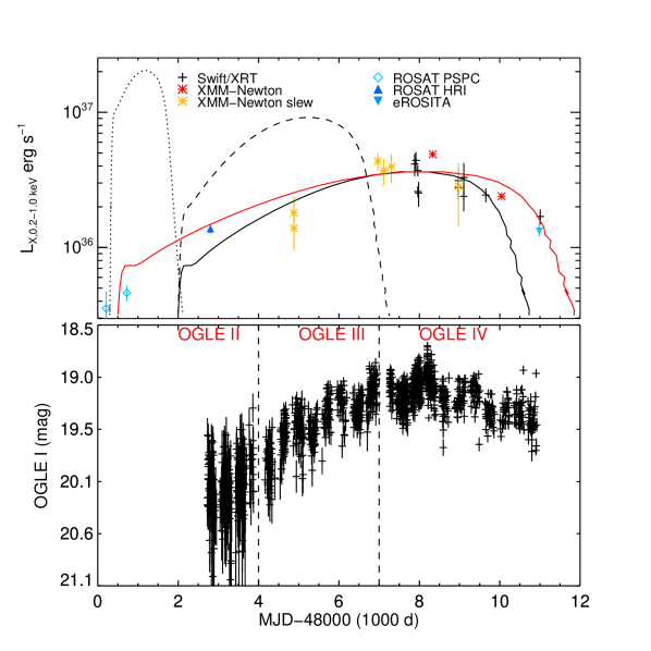
Figure 3: Left: OGLE finding chart, the red circle with 3″ radius is centered on the XMM-Newton 2013 detection, the blue circle with 1″ radius marks the location of J050526 based on the 2017 XMM-Newton detection after boresight correction. The most probable counterpart is located at the center of the image and is marked with a cyan circle. All other counterparts within 4.5″ of the XMM-Newton position are marked with various colours, with magenta being the least likely. Right - Top panel: X-ray light curve of J050526 based on all the available X-ray detections. The Y-axis corresponds to the absorption corrected luminosity (0.2-1.0 keV band) of the BB models presented in Table 1. Swift/XRT and ROSAT count-rates were converted adopting the spectral model parameters derived from the XMM-Newton/EPIC spectra. Overplotted are theoretical predictions of post-nova evolutionary tracks from Soraisam et al. (2016), and for WD masses of 0.9 M_⊙ (dotted line), 0.8 M_⊙ (dashed line) and 0.7 M_⊙ (solid black line), we also plot the 0.7 M_⊙ model stretched by 30% in time (red solid line). Right - Bottom panel: OGLE I band light curve of LMC510.12.65281 (cyan circle left panel). Data obtained during the OGLE-II, III & IV phase.

2.3 Long term X-ray variability

We now turn to studying the historic X-ray light-curve of the J050526 with data obtained over $\sim$30 years from multiple observatories. The first X-ray detection was made during the ROSAT all-sky survey in November 1990 (Voges et al., 1999). Additional ROSAT detections followed during pointed PSPC observations on 9 April 1992 (source 715; Haberl & Pietsch, 1999) and HRI observations on 19 December 1997 (source LMC 23; Sasaki et al., 2000). Apart from the 2 XMM-Newton pointed observations, J050526 has been detected 6 times in the XMM-Newton slew survey (Saxton et al., 2008). J050526 was also detected in 11 Swift/XRT pointings between 2011 and 2020 (Evans et al., 2014, 2020). To calculate average count rates for all Swift/XRT detections, we analyzed available data through the Swift science data centre following Evans et al. (2007, 2009). To convert count rates from all other instruments to unabsorbed $L_{X}$ in the 0.2-1.0 keV band we adopted the best fit BB model from XMM17 (see Table 1). At this point we comment on adopting a constant k${\rm T_{BB}}$ for the WD pseudophotosphere to convert count rates to unabsorbed $L_{\rm X}$. Unfortunately, the lack of observations with high statistics during the early states does not allow us to perform spectral fit to the data. However, it is expected from theory (see, e.g., Wolf et al., 2013) that k${\rm T_{BB}}$ evolves during the post nova phase. For low mass WD, k${\rm T_{BB}}$ can change by a factor 1.5 over 10s of years (Soraisam et al., 2016), which would result in an overestimate of $L_{\rm X}$ when assuming constant k${\rm T_{BB}}$ at earlier times. However, this could be compensated by an increased column density in earlier times, as has been suggested by observations of the initial evolution of other post novae (Page et al., 2010) such that we get a similar unabsorbed $L_{\rm X}$ for a slightly reduced k${\rm T_{BB}}$ with a bit higher column density.

During the course of the first all-sky survey (eRASS1) J050526 was monitored in May 2020 by the eROSITA instrument on board the Russian/German Spektrum-Roentgen-Gamma (SRG) mission (Merloni et al., 2012). Between MJD 58981.37 and 58989.37, J050526 was scanned 49 times accumulating a total exposure time of $\sim$1667 s. We extracted a combined spectrum from the five eROSITA CCD cameras with on-chip Al blocking filter. The other two cameras suffer from optical light leakage which requires more complicated calibration, before they can be used for reliable spectral analysis. We fitted the spectrum with the same black-body model as used for the XMM-Newton spectra. The best-fit parameters were determined to $N_{\rm{H}}$ LMC = 0 (upper limit 1.8$\times 10^{20}$ cm^-2) and k${\rm T_{BB}}$ = 85.6 $\pm$ 4 eV, which results in $L_{x}=1.32^{+0.23}_{-0.11}$$\times 10^{36}$ erg s^-1 (0.2-1.0 keV).

In Fig. 3 we present the resulting X-ray light-curve based on all available X-ray data. As we will discuss in $\S$3.2 this will enable comparison with available theoretical models.

2.4 Possible optical counterpart

We searched the available catalogues for possible optical counterparts. However, many optical surveys could not deliver the desired resolution and sensitivity (e.g. Massey, 2002; Zaritsky et al., 2004). Nevertheless, the region of interest was studied by the OGLE survey and several stars were detected within the X-ray error circle (Udalski et al., 2000).

For the field around J050526, OGLE provides more than 20 years of monitoring data. OGLE images are taken in the V and I filter pass-bands (B filter was also used during OGLE phase II), while photometric magnitudes are calibrated to the standard VI system (Udalski et al., 2015). There are a few possible optical counterparts located near the X-ray position (Fig. 3). For completeness, we extracted the optical light-curves of all 11 systems located within 4.5″ of the uncorrected X-ray position. We investigated all the extracted I band light-curves, and noted that among them only one showed evidence of significant variability (OGLE ID: LMC510.12.65281). The long-term optical variability seems to correlate well with the long-term evolution of the X-ray luminosity of the system (right panel of Fig. 3). In close binary SSSs, the optical light is dominated by the illuminated low-mass donor star and the accretion disk around the WD (Greiner, 1996), thus the optical light-curve provides strong evidence that this is the correct counterpart of J050526. The coordinates of the proposed OGLE counterpart are R.A. = 05^h05^m21$\aas@@fstack{s}$79 and Dec. = –68°45′37$\aas@@fstack{\prime\prime}$9 (J2000). The OGLE II photometric data obtained during the lowest flux state of the optical counterpart can provide an upper limit for the mass of the proposed counterpart (Udalski et al., 2000). Photometric values can be corrected for reddening, by adopting a Galactic extinction curve (Fitzpatrick, 1999). By using an $E(B-V)$ extinction value of 0.055 (Skowron et al., 2020) and the LMC distance module of 18.476 mag (Pietrzyński et al., 2019) we find absolute magnitudes of B$\sim$1.627, V$\sim$1.53 and I$\sim$1.47 (average during OGLE II phase); if we assume that the optical light originates exclusively from the star (neglecting both the accretion disk and irradiation), this is consistent with a main sequence star close to $2M_{\odot}$. We return to this point in $\S$3.2.

Given the binary nature of the system it is possible that a periodical signal due to the orbital motion is imprinted in the optical lightcurve. To test this we computed the Lomb-Scargle periodogram (VanderPlas, 2018) of the complete OGLE data-set. for completeness, we also limited our search to one year long chunks of data. We focused on periods between 0.01 d and 100 d. No periodic signal was identified, and the only peaks in the periodogram were consistent with the OGLE window function (1d, 0.5d, 0.33d and so on).

3 Discussion

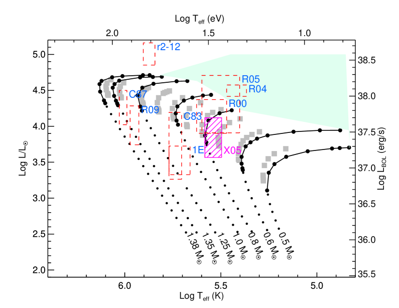
Figure 4: H-R diagram showing several SSSs; (R09) RXJ0925.7-4758; (C83) CAL 83; (1E) 1E 0035.4-7230; (R00) RX J0019.8+2156; (R04) RX J0439.8-6809; (R05) RX J0513.9-6951 (see Nomoto et al., 2007; Starrfield et al., 2004), (C87) CAL 87 (values corrected for obscuration; Ebisawa et al., 2001); r2-12 (Trudolyubov & Priedhorsky, 2008) and J050526 (X05) that we present in this paper and the spectral parameters of the NLTE model (we used 5$\times 10^{37}$ erg s^-1 as an upper limit for $L_{x}$). Also shown are the stable-burning models of Wolf et al. (2013) (gray squares), and the stable-burning (connected large black dots) and nova (small black dot) white dwarf models of Nomoto et al. (2007). The latter’s “red giant” or optically-thick wind regime (maximally-accreting) is denoted by the green shaded region.

3.1 The Nature of J050526

Examining the evolution of J050526 over the last 30 years, the source experienced over a ten-fold increase in luminosity between November 1990 and 2011, though initially rising only gradually over the first decade. In order to constrain the properties of the accreting WD undergoing this eruption, it is illustrative to compare the source radii found from our spectral fitting with that expected from theory. For cold, non-accreting carbon-oxygen WDs, the theoretical mass-radius relation gives (Panei et al., 2000):

$$\frac{R(M)}{R_{\odot}}=0.0126\left(\frac{\rm{M}}{\rm{M}_{\odot}}\right)^{-1/3}\left(1-\left(\frac{\rm{M}}{1.456M_{\odot}}\right)^{4/3}\right)^{1/2}$$ (1)

Looking first to our BB fits, we find that even at its greatest extent our best-fitting WD radius is consistent only with an extremely massive ($\gtrsim$1.4$M_{\odot}$), extremely compact WD (or perhaps a small region on the WD surface, see further discussion below). This is strongly contradicted, however, by the low (as derived from our black-body fits) luminosity and long timescale of the luminosity evolution observed for J050526– even at peak luminosity, the implied accretion rate in the steady-hydrogen burning regime ($\dot{m}=L/(\epsilon_{H}X)\approx 3.4\times 10^{-8}M_{\odot}$/yr, with $\epsilon_{H}\approx 6.4e18$ erg/g the energy release due to nuclear burning of hydrogen, and $X\approx 0.72$ the mass fraction of hydrogen) is well below the threshold for steady-burning at this mass ($\sim\rm{few}\times 10^{-7}M_{\odot}$/yr, Nomoto et al., 2007), and for such massive WDs at lower accretion rates, post-nova SSSs evolve on timescales measured in days, not years (Wolf et al., 2013). We conclude that in this case black-body models are inadequate; detailed NLTE WD atmospheric models are essential in interpreting the soft X-ray spectrum of J050526 (at least without additional constraints from multiwavelength data, see Skopal, 2015, for further discussion).

Turning to our NLTE fits (Table 1), we find approximate radius $\sim$15,000 km; substantially larger than even the lowest mass non-accreting carbon oxygen WDs. This is consistent (see Fig. 4), however, with the inflated photospheres expected in a WD which is undergoing residual nuclear-burning of hydrogen in its remaining envelope after a nova eruption (e.g., Wolf et al., 2013). Alternatively, this could be an indication of a magnetic WD, as such systems exhibit larger radii compared to non-magnetic ones (Suh & Mathews, 2000).

In the upper right panel of Fig. 3, we compare the observed X-ray luminosity evolution as measured with ROSAT, Swift, and XMM-Newton (0.2-1.0 keV band), with theoretical models of the post-nova hydrogen-burning SSS phase for a 0.7, 0.8, and 0.9 $M_{\odot}$ WD accreting $10^{-9}M_{\odot}$/yr (Wolf et al., 2013; Soraisam et al., 2016). The slow rise and subsequent relatively fast decline from a peak luminosity of $\approx 2.5\times 10^{37}$erg/s closely resembles the predicted evolution of a slowly accreting WD undergoing a post-nova SSS phase. In particular, we find that the model for a $0.7\leavevmode\nobreak\ M_{\odot}$ WD most closely resembles the observed luminosity evolution of J050526, although the predicted duration of the peak emission ($L_{x}\gtrsim\times 10^{36}\leavevmode\nobreak\ {\rm ergs^{-1}}$) exhibits a somewhat shorter timescale compared to the observed light curve.

Before continuing our comparison with numerical results, we must address two primary uncertainties in the post-nova models, namely, the mass-loss mechanism during the nova outburst, and mixing between the WD core and accreted matter. Wolf et al. used two prescriptions in their post-nova MESA models – super-Eddington wind (SEW), and Roche lobe (RL) overflow. The former is more appropriate for massive WDs ($\gtrsim 1\leavevmode\nobreak\ M_{\odot}$), which become super-Eddington early and thereby never expand to their bigger RL radii. Soraisam et al. (2016) used only the SEW models to construct the theoretical light curves since bright post-nova SSSs, which arise from massive WDs, are expected to be observed generally. On the other hand, the lower mass WDs tend to fill their RL radii before their luminosity becomes super-Eddington and thus, the RL overflow prescription may be better suited for such WDs. Theoretical light curves for these models are, however, not available. The wind prescription removes more mass than RL overflow, hence the SSS duration is longer in the latter case (by a factor $>5$ for 0.7$M_{\odot}$; see Wolf et al. 2013). Furthermore, mixing has not been incorporated in the MESA models. Mixing leads to a more violent outburst, which ejects more mass and results in a reduced amount of hydrogen remnant to burn and consequently, shortens the post-nova SSS duration. However, quantifying this effect is difficult (and beyond the scope of this paper). In Fig. 3 (upper right panel), the red curve shows the 0.7$M_{\odot}$ model light curve stretched by a factor 1.3, which, interestingly, matches the data well, indicating that a combination of the two uncertainties—mixing and mass-loss—can account for the discrepancy between the observations and model. Thus, all this evidence points to J050526 as likely a post-nova SSS. We cannot further constrain its nature without additional available models, which we therefore reserve for future work.

3.2 A post-nova SSS-irradiated donor?

Also requiring further study is the possibility that LMC510.12.65281 is the optical counterpart of J050526. If this is the case, what has caused its optical luminosity to rise and fall so closely in tandem with the post-nova SSS X-ray luminosity, long after what would have been the peak in the optical emission of the nova itself? If we naively interpret the emission as arising from the companion alone, its V magnitude and B-V colour are consistent with a $\sim$2$M_{\odot}$ main sequence or early subgiant star, however the strong evolution in its luminosity and its correlation with the soft X-ray flux suggest an additional component. During this time, the inferred WD photospheric radius is too large, and the accretion rate too low, for the disk luminosity to greatly exceed $\sim$$L_{\odot}$. At the same time, the necessarily falling density of the expanding nova ejecta would suggest it is unlikely that the rising optical luminosity could be powered by photoionization of this material by the WD.

Another possibility is that the residual nuclear-burning luminosity of the WD irradiates the donor, with a fraction of this flux consequently being re-emitted in the optical. Approximating the donor as spherically-symmetric, and assuming it is just filling its Roche lobe, from the vantage point of the WD it will subtend an area on the sky with an angular radius $\theta$, i.e.:

$$\tan(\theta)\approx\frac{R_{\rm{donor}}}{a}=\frac{0.49q^{2/3}}{0.6q^{2/3}+\ln(1+q^{1/3})}$$ (2)

where $R_{\rm{donor}}$ is the donor radius, $a$ is the separation between the donor and the WD, and their ratio depends only on the mass ratio $q=M_{\rm{donor}}/M_{\rm{WD}}$ (Eggleton, 1983). For $M_{\rm{WD}}\approx 0.7M_{\odot}$, a donor mass of 1–2$M_{\odot}$ gives q $\approx$ 1.43 – 2.85, $R_{\rm{donor}}/a\approx 0.41$–0.47, and $\theta\approx$ 0.39–0.44. This means the irradiated donor intercepts as much as $\pi\theta^{2}/4\pi\approx$ 4 – 5% of the post-nova SSS’s luminosity, only a fraction of which need be re-emitted by the donor’s envelope in the I band in order to account for the light curve of LMC510.12.65281. Notably, if we adopt a representative donor radius of $\sim$ 1– 2 $R_{\odot}$, we may also infer a binary orbital period of $\approx$0.2–0.6 days, comparable to the short term $\sim$0.5 magnitude optical variations seen throughout the OGLE light curve (recall Fig. 3). Before speculating further, however, follow-up optical spectroscopy will be essential in order to confirm the nature of LMC510.12.65281.

3.3 Origin of the 170s pulsational period

The high-frequency pulsations exhibited in the X-ray light curve of J050526 add a further commonality with most, if not all SSSs (see e.g., Ness et al., 2015), albeit with a slightly longer period than the 10 – 100s pulsations typically associated with this class. The origin of SSS pulsations remains a mystery, however the shortest period pulsations are generally argued to be associated with either the rotational period of the WD (e.g., Odendaal et al., 2014) or g-mode oscillations in the nuclear-burning envelope (Drake et al., 2003).

In the rotational period interpretation, the WD has been spun-up by accretion, and accreting matter is funneled by a strong magnetic field from the Keplerian disk toward the WD’s poles (the system is an intermediate polar). Such an interpretation has been put forward for the persistent supersoft source r2-12 in M31 (Kong et al., 2002), with a similar pulse period of $\sim$218 s (Trudolyubov & Priedhorsky, 2008). Assuming a Keplerian accretion disk, the torque induced onto the WD due to mass accretion will be maximum when the magnetospheric radius $R_{M}$ is equal to the co-rotation radius (i.e 43000 km). This is no different than the case of an accreting neutron star, where the torque due to mass accretion is $N_{\rm acc}=\dot{M}\sqrt{GM_{WD}R_{M}}$ (e.g. Vasilopoulos et al., 2018; Vasilopoulos et al., 2019). Thus the maximum spin-up rate due to accretion would be:

$$\dot{P}\sim-2.2\times 10^{-15}\rm{ss}^{-1}\leavevmode\nobreak\ \dot{M}_{19}I_{\rm{50}}^{-1}m_{\rm{WD}}^{2/3}P^{7/3}$$ (3)

where $I_{\rm{50}}$ is the WD’s moment of inertia in units of $10^{50}\leavevmode\nobreak\ g\leavevmode\nobreak\ cm^{-2}$, $\dot{M}_{19}$ is the mass accretion rate in units of $10^{19}\rm{g/s}$ and $m_{WD}$ the WD mass in units of $M_{\odot}$. As a crude approximation, we may take the WD as a constant density sphere within the cool WD radius $R(0.7M_{\odot})\approx 0.011R_{\odot}$ (recall equation 1), ignoring the much lower density envelope. This gives us $I_{50}\approx 3.4$ and an upper bound on $\dot{P}\sim-5\times 10^{-13}\rm{ss}^{-1}$, about 2000 lower than the observed $\dot{P}$ for J050526. Assuming that the periodic modulation is indeed due to rotation, an alternative origin for the period’s evolution may be that J050526 hosts a young contracting WD. This scenario has been proposed for other systems, and can produce the observed $\dot{P}$ for a range of WD masses with ages below 1 Myr (see Popov et al., 2018).

Otherwise, this would appear to leave g-mode oscillations in the nuclear-burning envelope as the only viable mechanism to explain the pulsations observed in J050526. It should be noted, however, that numerical models which have attempted to simulate such non-radial oscillations, driven by the sensitivity of nuclear-burning to compression (the $\epsilon$-mechanism) at the base of the envelope, have predicted much shorter period oscillations to be excited than are observed in known SSSs (Wolf et al., 2018). This problem remains in need of further investigation.

4 Conclusions

Largely disregarded upon its initial identification with ROSAT as a nondescript X-ray source, the $\sim$2013 soft X-ray peak and subsequent decline of J050526 have revealed it to be a remarkably long-lived post-nova SSS, with a WD mass below that common among other known SSSs but typical of the broader accreting WD population (e.g., Zorotovic et al., 2011). Indeed, J050526 is the longest-duration post-nova SSS yet confirmed as such (Ness et al., 2008; Henze et al., 2014), although amongst the known SSS population of e.g., M31 there are likely many long-lived post-novae awaiting further confirmation from long-term follow-up surveys (Orio, 2006; Henze et al., 2014; Soraisam et al., 2016). As such, J050526 provides an invaluable probe of the poorly-understood, but likely well-populated, long/soft/moderately faint segment of the parameter space of WD X-ray transients, and a natural laboratory for future X-ray pulsation and irradiation studies.

Data availability

X-ray data are available through the High Energy Astrophysics Science Archive Research Center heasarc.gsfc.nasa.gov. Other data underlying this article will be shared on reasonable request to the corresponding author. The eROSITA data are subject to an embargo period of 24 months from the end of eRASS1 cycle. Once the embargo expires the data will be available upon reasonable request to the corresponding author.

References

- Arnaud (1996) Arnaud K. A., 1996, in Jacoby G. H., Barnes J., eds, Astronomical Society of the Pacific Conference Series Vol. 101, Astronomical Data Analysis Software and Systems V. p. 17
- Chen et al. (2014) Chen H.-L., Woods T. E., Yungelson L. R., Gilfanov M., Han Z., 2014, MNRAS, 445, 1912
- Chen et al. (2015) Chen H.-L., Woods T. E., Yungelson L. R., Gilfanov M., Han Z., 2015, MNRAS, 453, 3024
- Denissenkov et al. (2017) Denissenkov P. A., Herwig F., Battino U., Ritter C., Pignatari M., Jones S., Paxton B., 2017, ApJ, 834, L10
- Dickey & Lockman (1990) Dickey J. M., Lockman F. J., 1990, ARA&A, 28, 215
- Drake et al. (2003) Drake J. J., et al., 2003, ApJ, 584, 448
- Ebisawa et al. (2001) Ebisawa K., et al., 2001, ApJ, 550, 1007
- Ebisawa et al. (2010) Ebisawa K., Rauch T., Takei D., 2010, Astronomische Nachrichten, 331, 152
- Eggleton (1983) Eggleton P. P., 1983, ApJ, 268, 368
- Evans et al. (2007) Evans P. A., et al., 2007, A&A, 469, 379
- Evans et al. (2009) Evans P. A., et al., 2009, MNRAS, 397, 1177
- Evans et al. (2014) Evans P. A., et al., 2014, ApJS, 210, 8
- Evans et al. (2020) Evans P. A., et al., 2020, ApJS, 247, 54
- Fitzpatrick (1999) Fitzpatrick E. L., 1999, PASP, 111, 63
- Greiner (1996) Greiner J., ed. 1996, Supersoft X-Ray Sources Lecture Notes in Physics, Berlin Springer Verlag Vol. 472, doi:10.1007/BFb0102238.
- Greiner et al. (1994) Greiner J., Hasinger G., Thomas H. C., 1994, A&A, 281, L61
- Haberl & Pietsch (1999) Haberl F., Pietsch W., 1999, A&AS, 139, 277
- Haberl et al. (2017) Haberl F., et al., 2017, A&A, 598, A69
- Henze et al. (2014) Henze M., et al., 2014, A&A, 563, A2
- Hitomi Collaboration et al. (2017) Hitomi Collaboration et al., 2017, Nature, 551, 478
- Huppenkothen et al. (2019) Huppenkothen D., et al., 2019, ApJ, 881, 39
- Kahabka & van den Heuvel (1997) Kahabka P., van den Heuvel E. P. J., 1997, ARA&A, 35, 69
- Kelly (2007) Kelly B. C., 2007, ApJ, 665, 1489
- Kong et al. (2002) Kong A. K. H., Garcia M. R., Primini F. A., Murray S. S., Di Stefano R., McClintock J. E., 2002, ApJ, 577, 738
- Kozłowski et al. (2013) Kozłowski S., et al., 2013, ApJ, 775, 92
- Krautter et al. (1996) Krautter J., Oegelman H., Starrfield S., Wichmann R., Pfeffermann E., 1996, ApJ, 456, 788
- Maoz et al. (2014) Maoz D., Mannucci F., Nelemans G., 2014, ARA&A, 52, 107
- Massey (2002) Massey P., 2002, ApJS, 141, 81
- Merloni et al. (2012) Merloni A., et al., 2012, arXiv e-prints, p. arXiv:1209.3114
- Ness et al. (2008) Ness J. U., Schwarz G., Starrfield S., Osborne J. P., Page K. L., Beardmore A. P., Wagner R. M., Woodward C. E., 2008, AJ, 135, 1328
- Ness et al. (2013) Ness J. U., et al., 2013, A&A, 559, A50
- Ness et al. (2015) Ness J. U., et al., 2015, A&A, 578, A39
- Nomoto et al. (2007) Nomoto K., Saio H., Kato M., Hachisu I., 2007, ApJ, 663, 1269
- Odendaal et al. (2014) Odendaal A., Meintjes P. J., Charles P. A., Rajoelimanana A. F., 2014, MNRAS, 437, 2948
- Orio (2006) Orio M., 2006, ApJ, 643, 844
- Page et al. (2010) Page K. L., et al., 2010, MNRAS, 401, 121
- Panei et al. (2000) Panei J. A., Althaus L. G., Benvenuto O. G., 2000, A&A, 353, 970
- Pietrzyński et al. (2019) Pietrzyński G., et al., 2019, Nature, 567, 200
- Popov et al. (2018) Popov S. B., Mereghetti S., Blinnikov S. I., Kuranov A. G., Yungelson L. R., 2018, MNRAS, 474, 2750
- Rauch & Deetjen (2003) Rauch T., Deetjen J. L., 2003, in Hubeny I., Mihalas D., Werner K., eds, Astronomical Society of the Pacific Conference Series Vol. 288, Stellar Atmosphere Modeling. p. 103 (arXiv:astro-ph/0403239)
- Rolleston et al. (2002) Rolleston W. R. J., Trundle C., Dufton P. L., 2002, A&A, 396, 53
- Sasaki et al. (2000) Sasaki M., Haberl F., Pietsch W., 2000, A&AS, 143, 391
- Saxton et al. (2008) Saxton R. D., Read A. M., Esquej P., Freyberg M. J., Altieri B., Bermejo D., 2008, A&A, 480, 611
- Skopal (2015) Skopal A., 2015, New Astron., 36, 116
- Skowron et al. (2020) Skowron D. M., et al., 2020, arXiv e-prints, p. arXiv:2006.02448
- Soraisam et al. (2016) Soraisam M. D., Gilfanov M., Wolf W. M., Bildsten L., 2016, MNRAS, 455, 668
- Starrfield et al. (2004) Starrfield S., Timmes F. X., Hix W. R., Sion E. M., Sparks W. M., Dwyer S. J., 2004, ApJ, 612, L53
- Sturm et al. (2013) Sturm R., et al., 2013, A&A, 558, A3
- Suh & Mathews (2000) Suh I.-S., Mathews G. J., 2000, ApJ, 530, 949
- Trudolyubov & Priedhorsky (2008) Trudolyubov S. P., Priedhorsky W. C., 2008, ApJ, 676, 1218
- Tsygankov et al. (2020) Tsygankov S. S., et al., 2020, A&A, 637, A33
- Udalski et al. (2000) Udalski A., Szymanski M., Kubiak M., Pietrzynski G., Soszynski I., Wozniak P., Zebrun K., 2000, Acta Astron., 50, 307
- Udalski et al. (2015) Udalski A., Szymański M. K., Szymański G., 2015, Acta Astron., 65, 1
- VanderPlas (2018) VanderPlas J. T., 2018, ApJS, 236, 16
- Vasilopoulos et al. (2013) Vasilopoulos G., Maggi P., Haberl F., Sturm R., Pietsch W., Bartlett E. S., Coe M. J., 2013, A&A, 558, A74
- Vasilopoulos et al. (2014) Vasilopoulos G., Haberl F., Sturm R., Maggi P., Udalski A., 2014, A&A, 567, A129
- Vasilopoulos et al. (2018) Vasilopoulos G., Haberl F., Carpano S., Maitra C., 2018, A&A, 620, L12
- Vasilopoulos et al. (2019) Vasilopoulos G., Petropoulou M., Koliopanos F., Ray P. S., Bailyn C. B., Haberl F., Gendreau K., 2019, MNRAS, 488, 5225
- Vasilopoulos et al. (2020) Vasilopoulos G., et al., 2020, MNRAS, 494, 5350
- Verner et al. (1996) Verner D. A., Ferland G. J., Korista K. T., Yakovlev D. G., 1996, ApJ, 465, 487
- Voges et al. (1999) Voges W., et al., 1999, A&A, 349, 389
- Werner & Dreizler (1999) Werner K., Dreizler S., 1999, Journal of Computational and Applied Mathematics, 109, 65
- Wilms et al. (2000) Wilms J., Allen A., McCray R., 2000, ApJ, 542, 914
- Wolf et al. (2013) Wolf W. M., Bildsten L., Brooks J., Paxton B., 2013, ApJ, 777, 136
- Wolf et al. (2018) Wolf W. M., Townsend R. H. D., Bildsten L., 2018, ApJ, 855, 127
- Woods & Gilfanov (2016) Woods T. E., Gilfanov M., 2016, MNRAS, 455, 1770
- Zaritsky et al. (2004) Zaritsky D., Harris J., Thompson I. B., Grebel E. K., 2004, AJ, 128, 1606
- Zorotovic et al. (2011) Zorotovic M., Schreiber M. R., Gänsicke B. T., 2011, A&A, 536, A42