Far-Field Automatic Speech Recognition

Abstract

The machine recognition of speech spoken at a distance from the microphones, known as far-field automatic speech recognition (ASR), has received a significant increase of attention in science and industry, which caused or was caused by an equally significant improvement in recognition accuracy. Meanwhile it has entered the consumer market with digital home assistants with a spoken language interface being its most prominent application. Speech recorded at a distance is affected by various acoustic distortions and, consequently, quite different processing pipelines have emerged compared to ASR for close-talk speech. A signal enhancement front-end for dereverberation, source separation and acoustic beamforming is employed to clean up the speech, and the back-end ASR engine is robustified by multi-condition training and adaptation. We will also describe the so-called end-to-end approach to ASR, which is a new promising architecture that has recently been extended to the far-field scenario. This tutorial article gives an account of the algorithms used to enable accurate speech recognition from a distance, and it will be seen that, although deep learning has a significant share in the technological breakthroughs, a clever combination with traditional signal processing can lead to surprisingly effective solutions.

I Introduction

Far-field, also called distant ASR is concerned with the machine recognition of speech spoken at a distance from the microphone. Such recording conditions are common for applications like voice-control of digital home assistants, the automatic transcription of meetings, human-to-robot communication, and several other more. In recent years far-field ASR has witnessed a great increase of attention in the speech research community. This popularity can be attributed to several factors. There is first the large gains in recognition performance enabled by Deep Learning (DL), which made the more challenging task of accurate far-field ASR come within reach. A second reason is the commercial success of speech enabled digital home assistants, which has become possible through progress in various fields, including signal processing, ASR and natural language processing (NLP). Finally, scientific challenges related to far-field noise and reverberation robust ASR, such as the REVERB challenge [1], the series of CHiME challenges [2, 3, 4, 5], and the ASpIRE challenge [6] exposed the task to a wide research audience and met with a lot of publicity. Conversely, those challenges have also helped to get a clearer picture as to which techniques and algorithms are helpful for far-field ASR.

The reason why far-field ASR is more challenging than ASR of speech recorded by a close-talking microphone is the degraded signal quality. First, the speech signal is attenuated when propagating from the speaker to the microphones, resulting in low signal power and often also low Signal-to-Noise Ratio (SNR). Second, in an enclosure, such as the living or a meeting room, the source signal is repeatedly reflected by walls and objects in the room, resulting in multi-path propagation, which causes a temporal smearing of the source signal called reverberation, much like multi-path propagation does in wireless communications. Third, it is likely that the microphone will capture other interfering sounds, in addition to the desired speech signal, such as the television or HVAC equipment. These sources of acoustic interference can be diverse, hard to predict, and often nonstationary in nature and thus difficult to compensate for. All these factors have a detrimental impact on ASR recognition performance.

Given these signal degradations, it is not surprising that quite different processing pipelines have emerged compared to ASR for close-talk speech. There is, foremostly, the use of a microphone array instead of a single microphone for sound capture. This allows for multi-channel speech enhancement, which has proven very successful in noisy reverberant environments. Second, the speech recognition engine is trained with data which represents the typical signal degradations the recognizer is exposed to in a far-field scenario. This robustifies the acoustic model (AM), which is the component of the recognizer which translates the speech signal into linguistic units. The following examples demonstrate the power of enhancement and acoustic modeling:

• The REVERB challenge data consists of recordings of the text prompts of the Wall Street Journal (WSJ) data set, respoken and rerecorded in a far-field scenario with a distance of 2-3 m between speaker and microphone array [1]. The challenge baseline ASR system, defined in 2014, which operates on a single channel microphone signal, achieved a Word Error Rate (WER) of 49%. Using a strong AM based on DL, the WER could be reduced to 22.2% [7, 8, 9], while the addition of a multi-microphone front-end and strong dereverberation brought the error rate down to 6.14% [10].

• The data set of the CHiME-3 challenge consists of recordings of the WSJ sentences in four different noise environments (bus, street, cafe, pedestrian area) [11]. The data was recorded using a tablet computer with six microphones mounted around the frame of the device. The baseline system reached a WER of 33%, while a robust back-end speech recognizer achieved 11.4% [12]. Finally, the multi-microphone front-end processing brought the error rate down to 2.7% [12].

• CHiME-5/6 consists of recordings of casual conversations among friends during a dinner party. The spontaneous speech, reverberation, and the large portion of times where more than one speaker is speaking simultaneously results in a WER of barely below 80% achieved by the baseline system. Using a strong back-end, approximately 60% WER is achieved [13], while the addition of multi-microphone source separation and dereverberation results in a WER of 43.2% [13]. Improvements in both front-end and back-end resulted in 30.5% WER in the follow-up CHiME-6 campaign [14].

The progress in ASR brought about by DL is well documented in the literature [15, 16, 17]. In this contribution we therefore concentrate on those aspects of acoustic modeling that are typical of far-field ASR. But those aspects, although improving the error rate a lot, proved to be insufficient to cope with high reverberation, low SNR and concurrent speech, as is typical of far-field ASR. This is because common ASR feature representations are agnostic to phase (a.k.a. spatial) information and are vulnerable to reverberation, i.e., the temporal dispersion of the signal over multiple analysis frames, and because it is difficult for a single AM to decide which speech source to decode, if multiple are present. Therefore, front-end processing for cleaning up the signals has been developed, including techniques for acoustic beamforming [18, 19], dereverberation [20, 21], and source separation/extraction [22]. All of those have been shown to significantly improve speech recognition performance, as can be seen in the examples above.

In the last years, neural networks (NNs) have challenged the traditional signal processing based solutions for speech enhancement [23, 24, 25], and achieved excellent performance on a number of tasks. However, those advances come at a price. The networks are notorious for their computational and memory demands, often require large sets of parallel data (clean and distorted version of the same utterance) for training, which have to be matched to the test scenario, and are “black box” systems, lacking interpretability by a human. In multi-channel scenarios, it is furthermore not obvious how to handle phase information. As a consequence researchers tried to combine the best of both worlds, i.e., to blend classic multi-channel signal processing with deep learning.

The purpose of this tutorial article is to describe the specific challenges of far-field ASR and how they are approached. We will discuss the general components of an ASR system only as much as is necessary to understand the modifications introduced in the far-field scenario. The organization of the paper is oriented along the processing pipeline of a typical far-field ASR as shown in Fig. 1. First, the signal is captured by an array of $M$ microphones. The signal model, which describes the typical distortions encountered, is given in Section II. Although recently good single-channel dereverberation [21] and source separation techniques have been developed [26, 24, 27], the use of an array of microphones instead of a single one has the clear advantage that spatial information can be exploited, which often leads to a much more effective suppression of noise and competing audio sources, as well as to better dereverberation performance. Dereverberation, acoustic beamforming and source separation/extraction techniques will be discussed in Section III.

Once the signal is cleaned up it is forwarded to the ASR back-end, whose task it is to transcribe the audio in a machine readable form. In far-field ASR it is particularly important to make the acoustic model robust against remaining signal degradations. We will explain in Section IV how this can be achieved by so-called multi-style training and by adaptation techniques. Section V discusses end-to-end approaches to ASR. In this rather new approach, the recognizer consists of a monolithic neural network, which directly models the posterior distribution of linguistic units given the audio. This paradigm has recently been extended to the far-field scenario, as we explain in that section.

We conclude this tutorial article with a summary and discuss remaining challenges in Section VI. We further provide pointers to software and databases in Section VII for those who want to gain some hands-on experience.

Figure 1: Typical far-field ASR system. Here, exemplarily with $M=3$ sensors, $I=2$ sources and additive noise.

This article primarily focuses on speech recognition accuracy, a.k.a. word error rate (WER), in far-field conditions as a criterion for success. Factors such as algorithmic latency or computational efficiency are only touched on in passing, although they are certainly of pivotal importance for the success of a technology in the market.

II Signal model and performance metrics

II-A Signal model

In a typical far-field scenario the signal of interest is degraded due to room reverberation, competing speakers, and ambient noise. Assuming an array of $M$ microphones, the signal at the $m$th microphone can be written as follows:

$$y_{m}[\ell]=\sum_{i=1}^{I}\left(a_{m}^{(i)}\ast s^{(i)}\right)[\ell]+n_{m}[\ell],$$ (1)

where $\ast$ is a convolution operation, $a_{m}^{(i)}[\ell]$ is the acoustic impulse response (AIR) from the origin of the $i$th speech signal $s^{(i)}[\ell]$ to the $m$th microphone, and $n_{m}[\ell]$ is the additive noise. Depending on the application, we might only be interested in one of the $I$ signals, say $s^{(i)}[\ell]$, while the remaining ones are considered unwanted competing audio signals.

In the following we assume that the AIR is time invariant, although it is well-known that movements of the speaker or changes in the environment, and even room temperature changes, cause a change of the AIR. Nevertheless, time invariance is a common assumption in ASR applications, justified by the fact, that an utterance, for which the AIR is assumed to be constant, is only a few seconds long.

However, the nonstationarity of the speech and noise signals has to be taken into account. When moving to a frequency domain representation we therefore have to use the Short-Time Fourier Transformation (STFT), i.e., apply the DFT to windowed segments of the signal. Typical window, also called frame, lengths are $25128\text{\,}\mathrm{m}\mathrm{s}$ and frame advances are $1032\text{\,}\mathrm{m}\mathrm{s}$.

When expressing the signal model of Eq. (1) in the STFT domain, it is important to note that, in a common setup, the AIR is much longer than the length of the analysis window. In a typical living room environment it takes $0.30.7\text{\,}\mathrm{s}$ for the AIR to decay to $-60\text{\,}\mathrm{d}\mathrm{B}$ of its initial value, which is considerably longer than the aforementioned window length. Then the convolution in Eq. (1) no longer corresponds to a multiplication in the STFT domain, but instead to a convolution over the frame index. To a good approximation [28, 29], Eq. (1) can be expressed in the STFT domain as

$$y_{m,t,f}=\sum_{i=1}^{I}\sum_{\tau=0}^{L-1}a_{m,\tau,f}^{(i)}s_{t-\tau,f}^{(i)}+n_{m,t,f},$$ (2)

where $a_{m,t,f}^{(i)}$ is a time-frequency representation of the AIR, called acoustic transfer function (ATF); $s_{t,f}^{(i)}$ and $n_{m,t,f}$ are the STFTs of the $i$th source speech signal and of the noise at microphone index $m$, frame index $t$, and frequency bin index $f$. Furthermore, $L$ denotes the length of the ATF in number of frames. Note that we used, in an abuse of notation, the same symbols for the time domain and frequency domain representations. This should not lead to confusion, because time domain signals have an argument, as in $y[\ell]$, while frequency domain variables have an index, as in $y_{t,f}$. The model of Eq. (2) strongly contrasts with the model for a close-talking situation, where $y_{t,f}=s_{t,f}+n_{t,f}$, or where even the noise term can be neglected.

When trying to extract $s_{t,f}^{(i)}$ from $y_{m,t,f}$, it comes to our help that multi-channel input is available, i.e., $m\in[1,\ldots,M]$. Defining the vector of microphone signals $\boldsymbol{\mathbf{y}}_{t,f}=\begin{bmatrix}y_{1,t,f}&\ldots,y_{M,t,f}\end{bmatrix}^{\mathrm{T}}$, we can write

$$\boldsymbol{\mathbf{y}}_{t,f}=\sum_{i=1}^{I}\sum_{\tau=0}^{L-1}\boldsymbol{\mathbf{a}}_{\tau,f}^{(i)}s_{t-\tau,f}^{(i)}+\boldsymbol{\mathbf{n}}_{t,f},$$ (3)

where $\boldsymbol{\mathbf{a}}_{t,f}^{(i)}$ and $\boldsymbol{\mathbf{n}}_{t,f}$ are similarly defined as $\boldsymbol{\mathbf{y}}_{t,f}$.

Fig.2 displays a typical AIR: it consists of three parts, the direct signal, early reflections and late reverberation caused by multiple reflections off walls and objects in the room. The early reflections are actually beneficial both for human listeners and for ASR. Its intelligibility is even better than that of the “dry” line-of-sight signal. After the mixing time, which is in the order of $50\text{\,}\mathrm{m}\mathrm{s}$, the diffuse reverberation tail begins. This late reverberation degrades human intelligibility and also leads to a significant loss in recognition accuracy of a speech recognizer. Thus, we split the ATF in an early and a late part:

$$\boldsymbol{\mathbf{y}}_{t,f} =\sum_{i=1}^{I}\boldsymbol{\mathbf{d}}_{t,f}^{(i)}+\sum_{i=1}^{I}\boldsymbol{\mathbf{r}}_{t,f}^{(i)}+\boldsymbol{\mathbf{n}}_{t,f},$$ (4)

where the early-arriving speech signals are given by

$$\boldsymbol{\mathbf{d}}_{t,f}^{(i)} =\sum_{\tau=0}^{\Delta-1}\boldsymbol{\mathbf{a}}_{\tau,f}^{(i)}s_{t-\tau,f}^{(i)}\approx\boldsymbol{\mathbf{h}}_{f}^{(i)}s_{t,f}^{(i)},$$ (5)

and the late-arriving speech signals are given by

$$\boldsymbol{\mathbf{r}}_{t,f}^{(i)} =\sum_{\tau=\Delta}^{L-1}\boldsymbol{\mathbf{a}}_{\tau,f}^{(i)}s_{t-\tau,f}^{(i)}.$$ (6)

Here, $\Delta$ is the temporal extent of the direct signal and early reflections, which is typically set to correspond to the mixing time. For example, $\Delta$ is set at $3$ when a frame advance is set at 16 ms. In Eq. (5), the desired signal is approximated by the product of a time-invariant (non-convolutive) ATF vector $\boldsymbol{\mathbf{h}}_{f}^{(i)}$ with the clean speech $s_{t,f}^{(i)}$, disregarding the spread of the desired signal over multiple analysis frames. Other works have tried to overcome this approximation by employing a convolutive transfer function model for the desired signal [30, 31].

Figure 2: An acoustic impulse response consists of the direct sound, early reflections and late reverberation.

Considering Eq. (4), the tasks of the enhancement stage can be defined as follows:

• Dereverberation (also known as deconvolution) aims at removing the late reverberation component from the observed mixture signal.

• The goal of source separation is to disentangle the mixture into its $I$ speech components, while

• Beamforming aims at extracting a target speech signal, which can be any of the $I$ sources, by projecting the input signal to the one-dimensional subspace spanned by the target signal, thereby diminishing signal components in other subspaces.

We will discuss each of the above tasks in detail in Section III.

II-B Performance metrics

Clearly, the ultimate performance measure depends on the application. For a transcription task it is the word error rate, while it is the success rate (high precision and recall) for an information retrieval task. However, when developing the speech enhancement front-end it is very helpful to be able to assess the quality of the enhancement with an instrumental measure which is independent of the ASR or a downstream NLP component. This will give not only smaller turnaround times in system development, but also gives more insight in how to improve front-end performance.

Clearly, speech quality and intelligibility is most informatively assessed by human listening experiments. But because these are too expensive and time consuming there is a whole body of literature devoted to how to measure speech quality or intelligibility by an “instrumental” measure. Measures, which have been originally developed to evaluate speech communication systems and which have found widespread use in speech enhancement are Perceptual Evaluation of Speech Quality (PESQ) [32] for speech quality and Short-Time Objective Intelligibility (STOI) for speech intelligibility [33]. Note that both measures are “intrusive”, which means that a clean reference signal is required. Please do also note that those measures are only moderately correlated with ASR performance, as has been empirically observed, e.g., in [12]. They are still useful in system development, but for a definite assessment of the benefits of an enhancement system for ASR, recognition experiments are indispensable.

For the evaluation of source separation performance the most common measure is the Signal-to-Distortion Ratio (SDR) [34]. It measures the ratio of the power of the signal of interest to the power of the difference between the signal of interest and its prediction (obtained by the source separation algorithm). Today, values of more than $10\text{\,}\mathrm{d}\mathrm{B}$ are not uncommon.

III Multi-channel speech enhancement

We now discuss enhancement techniques to address the aforementioned signal degradations. While linear and non-linear filtering approaches are developed for speech enhancement, the linear filtering has empirically been shown to be advantageous to estimate the desired signal $\boldsymbol{\mathbf{d}}_{t,f}^{(i)}$ in Eq. (3) from the observation $\boldsymbol{\mathbf{y}}_{t,f}$ in terms of WER reduction of far-field speech recognition [1, 2, 13]. This linear filtering leverages information the AM typically does not have access to, while not introducing time-dependent artifacts such as musical tones. On the other hand, the non-linear filtering approach has been shown to be useful for estimating statistics of signals, such as time-frequency dependent variances and masks of signals [23, 35], which are effectively used for estimating a linear filter.

A very general form of a (causal time-invariant) linear filter can be represented by a convolutional beamformer [36, 37, 31, 30]. It is defined as

$$\hat{d}_{1,t,f}^{(i)} =\sum_{\tau=0}^{L_{w}-1}\left(\boldsymbol{\mathbf{w}}_{\tau,f}^{(i)}\right)^{\mathrm{H}}\boldsymbol{\mathbf{y}}_{t-\tau,f},$$ (7)

where $\hat{d}_{1,t,f}^{(i)}$ is an estimate of $\boldsymbol{\mathbf{d}}_{t,f}^{(i)}$ at the $1$st microphone, $\boldsymbol{\mathbf{w}}_{\tau,f}^{(i)}=[w_{1,\tau,f}^{(i)},\ldots,w_{M,\tau,f}^{(i)}]^{\mathrm{T}}\in\mathbb{C}^{M\times 1}$ is a coefficient vector of the convolutional beamformer to be optimized for the estimation of $\hat{d}_{1,t,f}^{(i)}$, $L_{w}$ is the length of the convolutional beamformer, and $\smash{(\cdot)^{\mathrm{H}}}$ denotes transposition and complex conjugation. While many techniques have been developed for optimizing a convolutional beamformer [36, 31, 30], an approach decomposing it into a multi-channel linear prediction (MCLP) filter and a beamformer is widely used as a frontend for the far-field ASR. With $\Delta=1$ and by applying the distributive property, Eq. (7) can be rewritten as

$$\hat{d}_{1,t,f}^{(i)} =\underbrace{\left(\!\boldsymbol{\mathbf{w}}_{0,f}^{(i)}\!\right)^{\mathrm{H}}\vphantom{\Bigg{|}}}_{\text{Beamformer}}\underbrace{\left(\!\boldsymbol{\mathbf{y}}_{t,f}-\sum_{\tau=\Delta}^{L_{w}-1}\left(\!\boldsymbol{\mathbf{C}}_{\tau,f}^{(i)}\!\right)^{\mathrm{H}}\boldsymbol{\mathbf{y}}_{t-\tau,f}\!\right)\vphantom{\Bigg{|}}}_{\text{\lx@glossaries@gls@link{acronym}{MCLP}{\leavevmode MCLP} filter}}\!,\!\!$$ (8)

where $\boldsymbol{\mathbf{C}}_{\tau,f}^{(i)}\in\mathbb{C}^{M\times M}$ is a MCLP coefficient matrix satisfying $\boldsymbol{\mathbf{C}}_{\tau,f}^{(i)}\boldsymbol{\mathbf{w}}_{0,f}^{(i)}=-\boldsymbol{\mathbf{w}}_{\tau,f}^{(i)}$. Equation (8) highlights that a convolutional beamformer that estimates $\hat{d}_{1,t,f}^{(i)}$ can be decomposed into two consecutive linear filters: A MCLP filter [38] corresponding to the terms in the parentheses, and a (non-convolutional) beamformer $\boldsymbol{\mathbf{w}}_{0,f}^{(i)}$ [39, 40]. As will be discussed later, the MCLP filter can perform reduction of late reverberation, namely dereverberation. The beamformer, on the other hand, can perform reduction of noise, i.e., denoising, and extraction of a desired source from other competing sources, i.e., source separation.

The factorization in Eq. (8) allows us to use a cascade configuration for speech enhancement, i.e., dereverberation followed by denoising and source separation. This is advantageous because we can decompose the complicated enhancement problem into sub-problems that are easier to handle. Furthermore, it is shown that, under certain moderate conditions, even when we separately optimize dereverberation and beamforming, the estimate obtained by the cascade configuration is equivalent to (or can be even better than) that obtained by direct optimization of the convolutional beamformer in Eq. (7) [41].

Although both dereverberation and beamforming are well-known concepts from antenna arrays [39, 42], acoustic signal processing in a non-stationary acoustic environment requires additional efforts, such as estimation of time-varying statistics of temporally-correlated desired sources and noise, and “broadband” processing in the time-frequency domain [43, 44]. For this purpose, many techniques have been developed:

• For dereverberation, estimation and subtraction of the spectrum of the late reverberation has been employed, e.g., [45]. Also, MCLP filtering with delayed prediction and a time-varying Gaussian source assumption have been developed and shown effective for both single and multiple desired source scenarios [46, 47].

• For denoising, techniques for effectively estimating the time-varying statistics of the desired signal and the noise have been developed based on estimation of a time-frequency dependent mask. [18, 48].

• For source separation, sophisticated techniques for estimating masks of multiple competing sources have been developed. Modern techniques are even able to handle multiple sources in single-channel input [49, 25, 26].

While these techniques are well established in classical signal processing areas [50, 51, 52, 20], recently purely deep learning based solutions have challenged those solutions, e.g. [35, 23]. The advantage of the deep learning-based solutions is their powerful capability of modeling source magnitude spectral patterns over wide time frequency ranges, which were very difficult to handle by classical signal processing approaches. The deep learning approaches, however, are also notorious for being resource hungry and hard to interpret. Their training for speech enhancement tasks requires parallel data, i.e., a database which contains each speech utterance in two versions, distorted and clean, one serving as input to the network, and the other as training target. Reasonably, this can only be obtained by artificially adding the distortions to a clean speech utterance, leaving an unavoidable mismatch between artificially degraded speech in training and real recordings in noisy reverberant environments during test. Classical signal processing solutions are typically much more resource efficient and do not have this parallel data training problem. We will show for each of the three enhancement tasks how “neural network-supported signal processing” or “signal processing supported neural networks” can combine the advantages of both worlds, achieving high enhancement performance, being resource efficient and rendering parallel data unnecessary [53, 54, 55, 56, 57, 58, 59].

A typical processing pipeline for dereverberation, separation, and extraction is illustrated in Fig. 3.

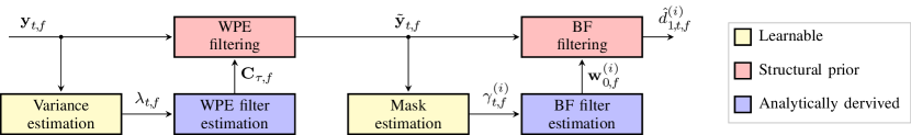
Figure 3: Overview of the enhancement system consisting of a neural network supported dereverberation module and a neural network supported or spatial clustering model supported beamforming module. The MCLP coefficient matrix $\boldsymbol{\mathbf{C}}_{\tau,f}$ as well as the time-varying variance $\lambda_{t,f}$ are speaker-independent as argued in the last paragraph of Sec. III-A. The BF filtering block may contain additional postfiltering to compensate for potential artifacts the beamformer may have produced.

III-A Dereverberation

The goal of dereverberation is to reduce the late reverberation $\boldsymbol{\mathbf{r}}_{t,f}^{(i)}$ from the observation $\boldsymbol{\mathbf{y}}_{t,f}$ in Eq. (4) while keeping the desired signal $\boldsymbol{\mathbf{d}}_{t,f}^{(i)}$ unchanged. Based on the decomposition in Eq. (8), we here highlight a technique based on MCLP filtering, referred to as Weighted Prediction Error (WPE) dereverberation [21, 46]. In the following, we first explain WPE dereverberation in the noiseless single source case, i.e., assuming $\boldsymbol{\mathbf{y}}_{t,f}=\boldsymbol{\mathbf{d}}_{t,f}^{(i)}+\boldsymbol{\mathbf{r}}_{t,f}^{(i)}$, and then explain its applicability to the noisy multiple source case at the very end of this section.

The core idea of WPE dereverberation is to predict the late reverberation of the desired signal from past observations. This late reverberation is then subtracted from the observed signal to obtain an estimate of the desired signal. Just as Eq. (8) indicates which past observations are used for prediction, Fig. 4 visualizes the past observations, the prediction delay and which frame of late reverberation is predicted. A unique characteristic of WPE is the introduction of the prediction delay $\Delta$, which corresponds to the duration of the direct signal and early reflections in Eq. (5). It avoids the desired signal being predicted from the immediately past observations, because this would destroy the short-time correlation typical of a speech signal. Thanks to this, the WPE can only predict the late reverberation and keep the desired signal unchanged.

Figure 4: WPE estimates a filter to predict the late reverberation in the current observation from the past observations (skipping $\Delta-1$ frames). The late reverberation is then subtracted from the current observation.

To deal with the time-varying characteristics of speech in the MCLP framework, WPE estimates the coefficient matrix $\boldsymbol{\mathbf{C}}_{\tau,f}^{(i)}$ based on maximum likelihood estimation. It is assumed that the desired signal $\boldsymbol{\mathbf{d}}_{t,f}^{(i)}$ follows a zero-mean circularly-symmetric complex Gaussian distribution with the unknown channel-independent time-varying variance $\lambda_{t,f}^{(i)}$ of the early-arriving speech signal:

$$p\left(\boldsymbol{\mathbf{d}}_{t,f}^{(i)}\right)=\mathcal{N}_{\mathbb{C}}\left(\boldsymbol{\mathbf{d}}_{t,f}^{(i)};\boldsymbol{\mathbf{0}},\lambda_{t,f}^{(i)}\boldsymbol{\mathbf{I}}_{M}\right),$$ (9)

where $\boldsymbol{\mathbf{d}}_{t,f}^{(i)}$ is obtained from MCLP filtering in Eq. (8) and $\boldsymbol{\mathbf{I}}_{M}$ is an $M\times M$-dimensional identity matrix. With this model, the objective to minimize becomes

$${\cal L}(\psi_{f}) =-\sum_{t}\log p\left(\boldsymbol{\mathbf{d}}_{t,f}^{(i)};\psi_{f}\right)$$

$$=\sum_{t}\frac{||\boldsymbol{\mathbf{y}}_{t,f}-\sum_{\tau=\Delta}^{L_{w}-1}\left(\boldsymbol{\mathbf{C}}_{\tau,f}^{(i)}\right)^{\mathrm{H}}\boldsymbol{\mathbf{y}}_{t-\tau,f}||_{2}^{2}}{\lambda_{t,f}}$$

$$\phantom{=}\quad+\sum_{t}M\log\lambda_{t,f}+\text{const.}$$ (10)

where $\psi_{f}$ is a set of parameters to be estimated at frequency $f$, composed of $\boldsymbol{\mathbf{C}}_{\tau,f}$ and $\lambda_{t,f}$ for all $\tau$ and $t$, and $||\cdot||_{2}$ denotes the Euclidean norm. Variations of the objective have also been proposed for better dereverberation performance by introducing sparse source priors [60, 61].

The minimization of the above objective leads to an iterative algorithm which alternates between estimating the time-varying variance $\lambda_{t,f}^{(i)}$ and the coefficient matrix $\boldsymbol{\mathbf{C}}_{\tau,f}^{(i)}$. The steps can be summarized as follows:

$$\text{Step 1)}\!\!\!\!\!\!\phantom{\mathbf{R}_{f}^{(i)}}\lambda_{t,f}^{(i)} =\frac{1}{\left(\delta+1+\delta\right)M}\sum_{\tau=t-\delta}^{t+\delta}\sum_{m}|d_{m,\tau,f}^{(i)}|^{2}\!,$$ (11)

$$\text{Step 2)}\!\!\!\!\!\!\phantom{\lambda_{t,f}^{(i)}}\mathbf{R}_{f}^{(i)} =\sum_{t}\frac{\boldsymbol{\mathbf{\bar{y}}}_{t-\Delta,f}\boldsymbol{\mathbf{\bar{y}}}_{t-\Delta,f}^{\mathrm{H}}}{\lambda_{t,f}^{(i)}} \!\!\!\!\!\!\!\in\mathbb{C}^{MK\times MK},$$ (12)

$$\mathbf{P}_{f}^{(i)} =\sum_{t}\frac{\boldsymbol{\mathbf{\bar{y}}}_{t-\Delta,f}\boldsymbol{\mathbf{y}}_{t,f}^{\mathrm{H}}}{\lambda_{t,f}^{(i)}} \!\!\!\!\!\!\!\in\mathbb{C}^{MK\times M},$$ (13)

$$\boldsymbol{\mathbf{\bar{C}}}_{f}^{(i)} =\left(\boldsymbol{\mathbf{R}}_{f}^{(i)}\right)^{-1}\mathbf{P}_{f}^{(i)} \!\!\!\!\!\!\!\in\mathbb{C}^{MK\times M},$$ (14)

where $\boldsymbol{\mathbf{\bar{y}}}_{t-\Delta,f}\in\mathbb{C}^{MK\times 1}$ is the stacked observation vector as depicted by the box on the left hand side of Fig. 4 and $\delta$ defines a temporal context.

In the variance estimation step in Eq. (11), $\lambda_{t,f}^{(i)}$ is updated dependent on the previous estimate of $\boldsymbol{\mathbf{C}}_{\tau,f}^{(i)}$, i.e., it is estimated as the variance of the signal dereverberated with $\boldsymbol{\mathbf{C}}_{\tau,f}^{(i)}$ according to the MCLP filter in Eq. (8). Often, smoothing by averaging over neighboring frames with a left context of $\delta$ and a right context of $\delta$ is introduced to reduce the variance of this variance estimate.

In the filter matrix estimation step in Eqs. (12)–(14), fixing $\lambda_{t,f}^{(i)}$ at its value estimated in the previous step makes Eq. (10) a simple quadratic form, and thus we can reach a global minimum by a closed-form update. Here, $\boldsymbol{\mathbf{R}}_{f}^{(i)}$ can be interpreted as an auto-correlation matrix of normalized stacked observation vectors. Further, $K=L_{w}-\Delta$ is the number of filter taps. Finally, Eq. (14) computes the stacked filter matrix

$$\boldsymbol{\mathbf{\bar{C}}}_{f}^{(i)}=\left[\left(\boldsymbol{\mathbf{C}}_{\Delta,f}^{(i)}\right)^{\mathrm{T}},\dots,\left(\boldsymbol{\mathbf{C}}_{L_{w}-1,f}^{(i)}\right)^{\mathrm{T}}\right]^{\mathrm{T}}$$ (15)

using the Wiener-Hopf equation.

This iterative algorithm may be started by initializing the time-varying variance $\lambda_{t,f}^{(i)}$ with that of the observation. Although this is a rather crude approximation, it typically converges within three iterations.

The use of a neural network further allows to estimate the time varying variance $\lambda_{t,f}^{(i)}$ within a single step avoiding the iterative estimation, and eases the transition towards online processing [56, 58]. In [56] a neural network is trained with a Mean Squared Error (MSE) loss to predict (the logarithm of) the time-varying variance $\lambda_{t,f}^{(i)}$ and applied to offline and block-online processing, while [58] extends this to frame-online processing.

In order to handle noisy multi-source cases, we slightly revise the goal of the WPE dereverberation to estimate a single set of coefficient matrices $\boldsymbol{\mathbf{C}}_{\tau,f}$ that can reduce the late reverberation $\boldsymbol{\mathbf{r}}_{t,f}^{(i)}$ for all $i$ at the same time, rather than estimating a different set of matrices $\boldsymbol{\mathbf{C}}_{t,f}^{(i)}$ separately for dereverberation of each source $i$. Existence of such a set of coefficient matrices is guaranteed by the multiple-input/output inverse theorem (MINT) [62] when $M\geq I$, $\boldsymbol{\mathbf{n}}_{t,f}=0$, and the acoustic transfer functions share no common zeros. The coefficient matrices can be estimated based on the objective of the WPE in Eq. (10), by setting $\lambda_{t,f}$ to represent the variance of the mixture of all $\boldsymbol{\mathbf{d}}_{t,f}^{(i)}$. Although $\boldsymbol{\mathbf{n}}_{t,f}=0$ is usually not satisfied within the far-field setting, due to the inherent robustness of the MCLP filtering, WPE works well with such additive noise.

While we discussed here WPE in some detail, because it has found widespread use in the ASR community, this is by no means the only approach to dereverberation. Instead of estimating the direct signal and early reflections, one can estimate the power spectral density of the late reverberation and subtract it from the observed signal, thereby achieving a dereverberating effect [45, 63]. Also, neural networks trained to estimate the nonreverberant signal from the observed reverberant one are very successful [10].

III-B Beamforming

Beamforming aims at reducing additive noise and residual reverberation from the observation. As in the decomposition in Eq. (8), a spatial filter $\boldsymbol{\mathbf{w}}_{0,f}^{(i)}$ (commonly referred to as beamformer) is used to obtain an estimate of the desired signal from the output of the WPE dereverberation. Consequently, we here define new variables which describe the signal components after WPE processing. Let us define the input of the beamformer as

$$\boldsymbol{\mathbf{\tilde{y}}}_{t,f} =\boldsymbol{\mathbf{d}}_{t,f}^{(1)}+\dots+\boldsymbol{\mathbf{d}}_{t,f}^{(I)}+\boldsymbol{\mathbf{\tilde{n}}}_{t,f}=\boldsymbol{\mathbf{d}}_{t,f}^{(i)}+\boldsymbol{\mathbf{\tilde{n}}}_{t,f}^{(i)},$$ (16)

where $\boldsymbol{\mathbf{\tilde{n}}}_{t,f}$ contains all residual reverberation and noise, and where $\boldsymbol{\mathbf{\tilde{n}}}_{t,f}^{(i)}$ collectively represents all the interference signal components from the viewpoint of speaker $i$: these are the remaining reverberation, the source signals other than the desired signal, ambient noise, and possible other deviations from $\boldsymbol{\mathbf{d}}_{t,f}^{(i)}$. In other words, Eq. (16) shows the decomposition from the perspective of speaker $i$ and not for all speakers. Then, the beamforming step is meant to remove all interferences $\boldsymbol{\mathbf{\tilde{n}}}_{t,f}^{(i)}$ from $\boldsymbol{\mathbf{\tilde{y}}}_{t,f}$ while keeping $\boldsymbol{\mathbf{d}}_{t,f}^{(i)}$ unchanged.

Most statistical beamforming approaches rely on estimated second order statistics, namely the spatial covariance matrices of the desired signal $\boldsymbol{\mathbf{\Phi}}_{\boldsymbol{\mathbf{d}}\boldsymbol{\mathbf{d}},f}^{(i)}$ and that of the interference ${\Phi}_{\boldsymbol{\mathbf{\tilde{n}}}\boldsymbol{\mathbf{\tilde{n}}},f}^{(i)}$. A beamforming algorithm is derived by defining an optimization criterion. A widely used approach is Minimum Variance Distortionless Response (MVDR) beamforming which minimizes the expected variance of the resultant interference subject to a distortionless constraint involving the ATF vector $\boldsymbol{\mathbf{h}}_{f}^{(i)}$ in Eq. (5). It is defined as

$$\boldsymbol{\mathbf{w}}_{0,f}^{(i)}=\operatorname*{argmin}_{\boldsymbol{\mathbf{w}}}\boldsymbol{\mathbf{w}}^{\mathrm{H}}\boldsymbol{\mathbf{\Phi}}_{\boldsymbol{\mathbf{\tilde{n}}}\boldsymbol{\mathbf{\tilde{n}}},f}^{(i)}\boldsymbol{\mathbf{w}}~{}~{}\text{s.t.}~{}~{}\boldsymbol{\mathbf{w}}^{\mathrm{H}}\boldsymbol{\mathbf{h}}_{f}^{(i)}=h_{1,f}^{(i)},$$ (17)

where $\boldsymbol{\mathbf{\Phi}}_{\boldsymbol{\mathbf{\tilde{n}}}\boldsymbol{\mathbf{\tilde{n}}},f}^{(i)}$ is the spatial covariance matrix of all interferences, assumed to be time-invariant, and $\smash{h_{1,f}^{(i)}}$ is the $1$st microphone element of $\smash{\boldsymbol{\mathbf{h}}_{f}^{(i)}}$. Thanks to the distortionless constraint, the beamformer keeps the desired signal unchanged, while reducing the additive distortions. The optimization problem in Eq. (17) results in

$$\boldsymbol{\mathbf{w}}_{0,f}^{(i)}=\frac{\left(\boldsymbol{\mathbf{\Phi}}_{\boldsymbol{\mathbf{\tilde{n}}}\boldsymbol{\mathbf{\tilde{n}}},f}^{(i)}\right)^{-1}\tilde{\boldsymbol{\mathbf{h}}}_{f}^{(i)}}{\left(\tilde{\boldsymbol{\mathbf{h}}}_{f}^{(i)}\right)^{\mathrm{H}}\left(\boldsymbol{\mathbf{\Phi}}_{\boldsymbol{\mathbf{\tilde{n}}}\boldsymbol{\mathbf{\tilde{n}}},f}^{(i)}\right)^{-1}\tilde{\boldsymbol{\mathbf{h}}}_{f}^{(i)}},$$ (18)

where $\tilde{\boldsymbol{\mathbf{h}}}_{f}^{(i)}$ is a relative transfer function (RTF) [64, 65] defined as the ATF vector normalized by its $1$st microphone component, i.e., $\tilde{\boldsymbol{\mathbf{h}}}_{f}^{(i)}={\boldsymbol{\mathbf{h}}}_{f}^{(i)}/h_{1,f}^{(i)}$. The RTF is a widely used representation to avoid scale ambiguity of ATF vector estimation.

Techniques for estimating the RTF vector $\tilde{\boldsymbol{\mathbf{h}}}_{f}^{(i)}$ have been developed, which in general require an estimate of a spatial covariance matrix $\boldsymbol{\mathbf{\Phi}}_{\boldsymbol{\mathbf{d}}\boldsymbol{\mathbf{d}},f}^{(i)}$ of the desired signal $\boldsymbol{\mathbf{d}}_{t,f}^{(i)}$ [18, 40]. Alternative objectives can also be used for beamforming, such as likelihood maximization with a time-varying Gaussian source assumption, similar to WPE, resulting in the weighted Minimum Power Distortionless response (wMPDR) beamformer [41], and maximization of expected output SNR resulting in maximum SNR beamformer (also called Generalized Eigenvalue Decomposition (GEV) beamformer) [66].

One way to estimate these covariance matrices is to select time frames in which just one signal component is active, e.g., the beginning of a recording where only noise is active. This approach is appropriate under the assumption that the corresponding signals are stationary. However, a better and more fine-grained approach is to use a time-frequency mask, $\gamma_{t,f}^{(i)}$, to decide for each time-frequency (TF) bin how well it corresponds to the target speaker or the interference. This leads to a covariance matrix calculation with time- and frequency-dependent masks $\gamma_{t,f}^{(i)}$:

$$\boldsymbol{\mathbf{\hat{\Phi}}}_{\boldsymbol{\mathbf{d}}\boldsymbol{\mathbf{d}},f}^{(i)} ={\sum_{t}\gamma_{t,f}^{(i)}\boldsymbol{\mathbf{\tilde{y}}}_{t,f}\boldsymbol{\mathbf{\tilde{y}}}_{t,f}^{\mathrm{H}}}\bigg{/}{\sum_{t}\gamma_{t,f}^{(i)}},$$ (19)

$$\boldsymbol{\mathbf{\hat{\Phi}}}_{\boldsymbol{\mathbf{\tilde{n}}}\boldsymbol{\mathbf{\tilde{n}}},f}^{(i)} ={\sum_{t}\sum_{i^{\prime}\neq i}\gamma_{t,f}^{(i^{\prime})}\boldsymbol{\mathbf{\tilde{y}}}_{t,f}\boldsymbol{\mathbf{\tilde{y}}}_{t,f}^{\mathrm{H}}}\bigg{/}{\sum_{t}\sum_{i^{\prime}\neq i}\gamma_{t,f}^{(i^{\prime})}}.$$ (20)

Conceptually, assuming that the selected TF bins indeed only contain the desired signal, $\boldsymbol{\mathbf{\hat{\Phi}}}_{\boldsymbol{\mathbf{d}}\boldsymbol{\mathbf{d}},f}^{(i)}\in\mathbb{C}^{M\times M}$ approximates the covariance matrix of $\boldsymbol{\mathbf{d}}_{t,f}^{(i)}$, and on a similar assumption, $\boldsymbol{\mathbf{\hat{\Phi}}}_{\boldsymbol{\mathbf{\tilde{n}}}\boldsymbol{\mathbf{\tilde{n}}},f}^{(i)}\in\mathbb{C}^{M\times M}$ approximates the covariance matrix of all interferences $\boldsymbol{\mathbf{\tilde{n}}}_{t,f}^{(i)}$.

Depending on the acoustic environment, the a priori knowledge for the given utterance, the number of speakers in the recording, and the available training data different ways to estimate the masks for each speaker are possible. The two predominant approaches for mask estimation are unsupervised spatial clustering and neural network-based mask estimation and are explained in the following section.

III-C Mask estimation for denoising, single source extraction, and source separation

The goal of a mask estimator is to estimate a presence probability mask for each speaker and for noise. This section first describes unsupervised spatial clustering approaches for single- and multi-speaker scenarios and then continues with neural network-based approaches again for single- and multi-speaker scenarios.

III-C1 Unsupervised spatial clustering

Unsupervised spatial clustering is a technique used to assign each TF bin to a particular class based solely on spatial cues, i.e., phase and level differences between microphone channels that provide information about the direction of sound with respect to the microphone array. A class then models the different speakers characterized by different locations or noise with more diffuse characteristics. Assuming that the speakers speak from different locations, it is possible to separate the microphone signals into speech signals of the different speakers by clustering the spatial cues [67].

To do so, one typically formulates a statistical model which consists of a class-dependent distribution for each source $i$ and an additional noise class which is here indexed by $i=I+1$:

$$p(\boldsymbol{\mathbf{\tilde{y}}}_{t,f})=\sum_{i=1}^{I+1}p(\boldsymbol{\mathbf{\tilde{y}}}_{t,f}|\boldsymbol{\mathbf{\theta}}^{(i)})p(z_{t,f}{=}i),$$ (21)

where $z_{t,f}$ is the hidden class affiliation variable, and $\boldsymbol{\mathbf{\theta}}^{(i)}$ summarizes the class-dependent parameters. Typical class-dependent distributions are the complex Watson distribution [68], complex Bingham distribution [69], or the complex angular central Gaussian distribution [70]. The parameters and the masks are then obtained through an Expectation-Maximization (EM) algorithm in which the E-step and the M-step alternate. In the M-step, the class-dependent parameters are updated. In the E-step, the masks $\smash{\gamma_{t,f}^{(i)}=p(z_{t,f}{=}i|\boldsymbol{\mathbf{\tilde{y}}}_{t,f})}$, which here correspond to posterior probabilities, are obtained using Bayes’ rule:

$$\gamma_{t,f}^{(i)}=\frac{p(z_{t,f}{=}i)\,p(\boldsymbol{\mathbf{\tilde{y}}}_{t,f}|\boldsymbol{\mathbf{\theta}}^{(i)})}{\sum_{i^{\prime}=1}^{I+1}p(z_{t,f}{=}i^{\prime})\,p(\boldsymbol{\mathbf{\tilde{y}}}_{t,f}|\boldsymbol{\mathbf{\theta}}^{(i^{\prime})})}.$$ (22)

In a single-speaker scenario, where one just wishes to distinguish between target speaker and noise, one can use spatial clustering with $I=1$. To name an example, the winning system of the CHiME 3 robust speech recognition challenge employed such an unsupervised clustering approach with $I=1$ successfully to single-speaker recordings [71]. In case of a multi-source scenario, $I$ has to be set to the number of speakers in the mixtures, which either has to be known a-priory, or estimated separately. The consecutive steps, e.g., beamforming as in Fig. 3 are then repeated for each speaker.

III-C2 Neural network-based mask estimation

In contrast, mask estimation networks are trained with a supervision signal. To discuss neural network-based approaches, we first introduce a neural mask estimator as used in neural network-based beamforming in the following. We then introduce SpeakerBeam as a speaker-informed mask estimator. Lastly, we introduce neural network-based blind source separation approaches.

For neural network-based mask estimation, a supervision signal such as an ideal binary mask (IBM) [72] is first extracted on each training mixture. To do so, one needs access to the speech images and the noise image, i.e., each individual speech component and the noise component at the microphones, separately:

$$\text{IBM}_{t,f}^{(i)} =\begin{cases}1,&\text{for }\big{\|}\boldsymbol{\mathbf{d}}_{t,f}^{(i)}\big{\|}_{2}^{2}>\big{\|}\boldsymbol{\mathbf{d}}_{t,f}^{(i^{\prime})}\big{\|}_{2}^{2}\,\forall\,i^{\prime}\neq i\\ 0,&\text{otherwise},\end{cases}$$ (23)

where $i$ corresponds to the source index. This definition can be extended to an additional noise class by treating the oracle noise signal as $\boldsymbol{\mathbf{d}}^{(I+1)}:=\boldsymbol{\mathbf{\tilde{n}}}_{t,f}$. Fig. 5 illustrates the underlyinging signal components and the corresponding IBM with an additional noise class. Further definitions of oracle masks suitable for supervision can be found in, e.g., [73, 74].

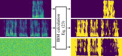
Figure 5: Visualization of the spectrograms of the underlying images $\boldsymbol{\mathbf{d}}_{t,f}^{(1)}$, $\boldsymbol{\mathbf{d}}_{t,f}^{(2)}$, and $\boldsymbol{\mathbf{\tilde{n}}}_{t,f}$ on the left and the ideal binary masks $\text{IBM}_{t,f}^{(1)}$, $\text{IBM}_{t,f}^{(2)}$, and $\text{IBM}_{t,f}^{(3)}$ on the right. Bright colors indicate higher values.

Then, depending on the particular use-case, a neural network can be trained with such a supervision signal. The different use-cases are illustrated in Fig. 6.

Figure 6: Processing flow for different use-cases of a mask estimator. The corresponding interference mask to calculate the interference covariance matrix in Eq. (20) is not shown for brevity.

Separate speech from noise

One can now train a neural network with, e.g., log-amplitude spectrogram features as input, to predict a speech mask and a noise mask by providing noisy speech training data from various speaker and the corresponding IBMs or clean speech signals. Since speech and noise have different spectro-temporal characteristics, a neural network can distinguish between these signals very well. An exemplary training criterion is the binary cross entropy between the estimated mask $\gamma_{t,f}^{i}$ and the corresponding oracle $\text{IBM}_{t,f}^{(i)}$.

This mask estimation procedure with a subsequent beamforming step led to dramatic WER reductions, e.g., in the CHiME 3/4 challenges [74, 75]. Often, these masks are estimated independently for each channel and then pooled over all channels such that a single mask can be used, e.g., in Eq. (20).

Extract a single speaker from a mixture

In many practical applications one is interested in one target speaker in a mixture, e.g., the speaker who is actually interacting with the digital home assistant. While dealing with speech mixtures, simply training a neural network to extract the target speaker is not possible because both the target speech and interference signal have similar spectro-temporal characteristics. However, if additional information about the target speaker is available, a neural mask estimator can be informed about speaker-dependent characteristics. These characteristics may stem from a separate adaptation utterance or from the wake-up keyword. In the SpeakerBeam framework [76, 77] a sequence-summarizing neural network [78] which captures the speaker-dependent characteristics is jointly trained with a mask estimation network which uses these characteristics as additional features to estimate a target speaker mask and an interference mask. VoiceFilter implements this approach with a Convolutional Neural Network (CNN) architecture [79].

Separate multiple speakers and noise

While, in a single-speaker scenario, a mask estimator only needs to distinguish between speech and non-speech time frequency bins (compare Sec. III-C2), source separation approaches have to solve the following problem: given the observation the algorithm should yield a mask for each speaker as well as an additional noise mask. For quite some time it has been complicated to do this with neural networks due to the permutation problem: while the order in which the speakers appear at the different output channels of the system is unpredictable, a loss function which assumes a particular order can result in misleading gradients. While the spatial clustering model in Eq. (21) is naturally permutation invariant (switching speaker indices does not change the likelihood), permutation invariant losses for neural networks appeared just recently.

Kolbaek et al. formulated a way to turn any loss function, e.g., Cross Entropy (CE), into a permutation invariant loss function [26]: the original loss is calculated for every possible permutation. Then, only the minimal loss is used for back-propagation, e.g.:

$$J =\operatorname*{argmin}_{\Pi}\sum_{i=1}^{I+1}\operatorname*{CE}_{t,f}\left(\gamma_{t,f}^{(\Pi(i))},\text{IBM}_{t,f}^{(i)}\right),$$ (24)

where $\Pi$ is a permutation of $(1,\dots,I+1)$. A neural network with $I+1$ mask outputs can now be trained with such a Permutation Invariant Training (PIT) loss. The estimated masks $\gamma_{t,f}^{(i)}$ can then be used, e.g., for beamforming. In its original formulation the network architecture of a PIT system depends on the maximum number of speakers expected in a mixture. The system can be trained in such a way that some output channels are empty when there are less speakers.

Fundamentally differently, Deep clustering, while pioneering this area, used a neural network to calculate embedding vectors for each time frequency bin [24]. The loss, as any typical embedding loss, is designed in such a way that the embedding vectors belonging to the same class move closer together while the embedding vectors of different classes move further apart. Naturally, such a formulation is permutation invariant in itself. The embedding vectors can then be used for clustering yielding masks in a similar way as explained in the clustering approach before. Interestingly, at least the embedding network is then independent of the number of speakers in a mixture [24].

III-C3 Comparison of spatial and spectral approaches and integrations thereof

The main advantage of spatial clustering models over neural network-based mask estimation is the interpretability of the underlying stochastic dependencies. Closely related, this interpretability allows to incorporate a priori knowledge by modifying the parameter updates, e.g., [80] uses externally provided time annotations for the CHiME 5 database. Due to the spatial features, it exploits spatial selectivity and, as long as the spatial properties of each source are distinct enough, is able to produce meaningful separation results. Since no training phase is involved, this unsupervised clustering approach naturally generalizes well to unseen conditions.

One drawback of the spatial clustering approaches is, that it is most suited for offline processing. Although quite a few online or block-online clustering approaches had been proposed, these did not find a lot of application in far-field ASR challenges yet. Moving sources, if no online algorithm is used, can only be handled to some extent: small head movements can still be captured in the class dependent parameters. Larger movements, however, invalidate the underlying model assumptions. Further, since clustering is often performed independently across frequency bins, a frequency permutation problem arises [81]: from one frequency bin to another the spatial clustering solution may have resulted in switched speaker indices. This frequency permutation problem is independent of the aforementioned global permutation problem when discussing PIT.

In contrast to the spatial clustering approaches, neural network-based approaches rely on spectral cues and process all frequency bins jointly. Therefore, a frequency permutation problem does not occur. Quite remarkably, the neural network-based separation models learn relations from training databases and tend to perform better with an ever increasing amount of training data.

However, alongside this comes their biggest limitation: depending on the variability of the training data, the models have limited generalizability to unseen conditions, e.g., Yu et al. demonstrated that the performance already degrades significantly when switching from English to Danish [82]. The training corpus needs to contain the mixed speech as well as access to the clean sources to be able to compute gradients. A notable exception are unsupervised approaches to train a neural network-based source separator [83, 84, 85]. Further, most neural network-based approaches are single-channel. Even when multi-channel features are employed [86], in which way those contribute to better separation performance is far from understood.

By no means these approaches are mutually exclusive. Judging by the aforementioned advantages and disadvantages, both methods are highly complementary, e.g., [87] proposed to combine neural network-based mask estimation with spatial clustering for speech enhancement, while [55, 88] proposed an integration of Deep Clustering and spatial clustering for multi-talker scenarios.

III-D Front-end overview

The entire front-end system is now composed of dereverberation, mask estimation, and beamforming. An established configuration is depicted in Fig. 3. The optimal processing order, as demonstrated in [7] for conventional beamforming and in [89] for neural network supported beamforming turns out to be applying WPE on the multi-channel signal first and then applying the beamforming step on the dereverberated signal.

Spatial clustering based source separation approaches profit in particular from a preceding WPE dereverberation (experimental results in [80]) since the sparseness assumption, which implies that different speakers populate different TF bins, is much better fulfilled for less reverberant speech. Further experiments also report improved separation performance with neural network-based separation methods [90]. However, it is worth to acknowledge that a publication which clearly tracks down the gains of better source separation due to better dereverberation is still missing.

In Fig. 3 the variance estimation network and the mask estimation network conceptually perform a similar task (at least in the single-speaker scenario). Thus, it might be worth investigating if both models can be fused into a single model with two different outputs. Further, for practical reasons, the mask estimation network often operates on the observation signal $\boldsymbol{\mathbf{y}}_{t,f}$ to avoid needing to train on dereverberation results.

From a machine learning perspective, it is worth highlighting that the building blocks in Fig. 3 are very differently motivated: the filtering blocks can be seen as structural priors motivated by an a priori understanding of field experts. The filter coefficient estimation blocks are derived analytically from separate optimization criteria, and the variance estimation neural network as well as the mask estimation neural network are trained independently with gradient descent on a separate training database. More recently, it has been demonstrated that the neural networks can also be trained with gradients from a downstream task [59, 57] (compare Sec. V).

IV ASR back-end

To achieve high ASR performance in a far-field scenario, we need not only employ a powerful speech enhancement front-end but also design carefully the ASR back-end. The ASR back-end used for far-field ASR has essentially the same structure as a general back-end used for recognition of clean speech. Those interested can find an overview of legacy ASR systems in [91], while [15, 16, 17] describe general ASR in the era of deep learning. However, several elements need careful consideration when dealing with far-field ASR. In this section, we will first briefly review a general ASR back-end and then emphasize the key components and design choices that are most relevant for far-field ASR.

IV-A Overview of a general ASR back-end

The goal of the ASR back-end is to find the most likely word sequence, $\boldsymbol{\mathbf{\hat{v}}}$, given a sequence of observed speech features $\boldsymbol{\mathbf{O}}$. Here for generality, the speech features can be derived either from clean speech, microphone observations or enhanced speech, as described in Section III. The task of ASR is formulated with the Bayes decision theory as

$$\boldsymbol{\mathbf{\hat{v}}}=\operatorname*{argmax}_{\boldsymbol{\mathbf{v}}\in\mathcal{V}}p\left(\boldsymbol{\mathbf{v}}|\boldsymbol{\mathbf{O}}\right),$$ (25)

where $\boldsymbol{\mathbf{O}}=(\boldsymbol{\mathbf{o}}_{1},\ldots,\boldsymbol{\mathbf{o}}_{t},\ldots,\boldsymbol{\mathbf{o}}_{T})$ is a sequence of speech features, $\boldsymbol{\mathbf{o}}_{t}\in\mathbb{R}^{D}$, is a feature vector for frame $t$, $\boldsymbol{\mathbf{v}}=(v_{1},\ldots,v_{j},\ldots,v_{J})$ is a $J$-length word sequence, $v_{j}\in\mathcal{V}$ is a word at position $j$, and $\mathcal{V}$ is the set of possible words, called vocabulary. Since it is complex to deal with $p(\boldsymbol{\mathbf{v}}|\boldsymbol{\mathbf{O}})$ directly, the problem is usually rewritten using the Bayes theorem as,

$$\boldsymbol{\mathbf{\hat{v}}}=\operatorname*{argmax}_{\boldsymbol{\mathbf{v}}\in\mathcal{V}}p\left(\boldsymbol{\mathbf{O}}|\boldsymbol{\mathbf{v}}\right)p(\boldsymbol{\mathbf{v}}),$$ (26)

where the likelihood function $p(\boldsymbol{\mathbf{O}}|\boldsymbol{\mathbf{v}})$ is called the acoustic model (AM) and the prior distribution $p(\boldsymbol{\mathbf{v}})$ is the language model (LM) [92]. Note that some recent end-to-end ASR systems described in Section V aim at directly modeling $p(\boldsymbol{\mathbf{v}}|\boldsymbol{\mathbf{O}})$.

Figure 7: Schematic diagram of a general ASR back-end.

Fig. 7 depicts a general ASR back-end with its main components, i.e., the feature extraction module, the AM and the language model, which are briefly described below.

IV-A1 Feature extraction

The first component of an ASR back-end is a feature extraction module that converts the time domain signal $\hat{d}_{1}[l]$ into speech feature $\boldsymbol{\mathbf{o}}_{t}$ more suitable for ASR. There has been a lot of research on designing robust features for ASR. However, the simple log-Mel filterbank (LMF) coefficients are widely used both for general and far-field ASR. LMF coefficients are obtained by computing the power spectrum of the time-domain signal using a STFT, then applying a Mel filter to emphasize low-frequency components of the spectrum. Finally, the dynamic range is compressed using the logarithm operation as,

$$o_{t,\nu} =\text{Feat}\left([\hat{d}_{t,1},\ldots,\hat{d}_{t,f},\ldots,\hat{d}_{t,F}]^{\mathrm{T}}\right),$$

$$=\text{MVN}\Bigg{(}\log\Big{(}\sum_{f}b_{\nu,f}|\hat{d}_{t,f}|^{2}\Big{)}\Bigg{)},$$ (27)

where Feat denotes the feature extraction process. Further, $\hat{d}_{t,f}$ is the STFT coefficient of the enhanced speech, $F$ is the number of frequency bins, $b_{\nu,f}$ represents the Mel filterbank associated with the $\nu$-th channel, and $\text{MVN}(\cdot)$ represents the mean and variance normalization (MVN) operation. Note that in general the parameters of the STFT (window type, length and overlap) used for speech enhancement and recognition differ. Therefore, the speech enhancement front-end usually converts the signals back to the time domain before doing feature extraction for ASR. The features are often normalized with MVN to have zero-mean and unit variance using statistics computed either for each utterance or over the whole training data set.

IV-A2 Acoustic model

The AM employs phonemes as a basic unit of speech sounds. In this section, we focus our discussion on Hidden Markov Model (HMM) based AMs, where each phoneme is associated with a HMM that models the dynamic evolution of speech within that phoneme [92, 93]. An HMM representing the whole word sequence is constructed from several phoneme HMM s using a pronunciation dictionary to map each word to a phoneme sequence. HMM based AMs make the conditional independence assumption, according to which an observed feature vector only depends on the current state and is independent of neighboring HMM states. This gives the following expression for the likelihood,

$$p\left(\boldsymbol{\mathbf{O}}|\boldsymbol{\mathbf{v}}\right)=a_{\sigma_{0},\sigma_{1}}p(\boldsymbol{\mathbf{o}}_{1}|\sigma_{1})\prod_{t=2}^{T}p(\boldsymbol{\mathbf{o}}_{t}|\sigma_{t})a_{\sigma_{t-1},\sigma_{t}},$$ (28)

where $\sigma_{t}$ is an HMM state at time $t$, $a_{\sigma_{t},\sigma_{t+1}}$ is the transition probability between state $\sigma_{t}$ and $\sigma_{t+1}$, $a_{\sigma_{0},\sigma_{1}}$ is the initial state probability, and $p(\boldsymbol{\mathbf{o}}_{t}|\sigma_{t})$ is the emission probability.

In legacy systems, the emission probability was modeled with a Gaussian Mixture Model (GMM). More recent systems use a Deep Neural Network (DNN) instead and are called DNN-HMM hybrid systems. Let $\boldsymbol{\mathbf{g}}(\boldsymbol{\mathbf{o}}_{t};\boldsymbol{\mathbf{\theta}})$ be the $\Sigma$-dimensional softmax output vector of a DNN AM with parameters $\boldsymbol{\mathbf{\theta}}$, where $\Sigma$ is the total number of HMM states, and $g_{\sigma}(\boldsymbol{\mathbf{o}}_{t};\boldsymbol{\mathbf{\theta}})$ is the output associated with HMM state $\sigma$. $g_{\sigma}(\boldsymbol{\mathbf{o}}_{t};\boldsymbol{\mathbf{\theta}})$ can be interpreted as a posterior probability $p(\sigma|\boldsymbol{\mathbf{o}}_{t})$, which can be be converted into a pseudo likelihood using Bayes rule as [15]

$$p(\boldsymbol{\mathbf{o}}_{t}|\sigma) \propto\frac{p(\sigma|\boldsymbol{\mathbf{o}}_{t})}{p(\sigma)},$$

$$=\frac{g_{\sigma}(\boldsymbol{\mathbf{o}}_{t};\boldsymbol{\mathbf{\theta}})}{p(\sigma)},$$ (29)

where a prior probability $p(\sigma)$ is derived from the statistics of the training data set.

There has been much research on designing appropriate network architectures for $g_{\sigma}(\boldsymbol{\mathbf{o}}_{t};\boldsymbol{\mathbf{\theta}})$. The choice for a specific architecture foremostly depends on latency constraints during inference time and the amount of available training data. It is a fast-evolving research field with new results claiming state-of-the-art performance due to often only slight modifications of the architecture being published almost on a weekly basis. Equally important is the choice of training hyperparameters and schemes. Both need extensive tuning for a fair comparison among architectures but this is often not possible due to a limited compute budget. In general, a solid baseline architecture are time delay neural networks (TDNNs) [96] or convolutional neural networks in general (e.g. [97]) possibly followed by some (bi-directional) Long-Short Term Memory (LSTM) layers [98]. Variants of this architecture have been employed successfully in the latest CHiME challenges. Recently, architectures with self-attention [99], often referred to as transformers, have shown competitive results on several benchmark tasks [100, 101].

IV-A3 Language model

The language model (LM) provides the prior probability of a word sequence. There exist N-gram LMs and neural LMs such as Recurrent Neural Network (RNN) LM [102]. The LM is trained on a large text corpus, and, unlike the other components of the ASR back-end, it is not affected by the acoustic conditions such as noise or reverberation. It can thus be very effective to improve the performance of far-field ASR when the language is well constrained such as for read speech tasks [71, 103]. However, for conversational situations, it is more difficult to model the speech content and thus the LM appears less effective [104].

IV-A4 Training procedure

Building an ASR back-end requires training the AM with speech training data and the associated transcriptions. The goal of the training is finding the DNN parameters, $\boldsymbol{\mathbf{\theta}}$, which optimize a training criterion as,

$$\boldsymbol{\mathbf{\hat{\theta}}}=\operatorname*{argmax}_{\boldsymbol{\mathbf{\theta}}}\sum_{u}\mathcal{C}\left(\boldsymbol{\mathbf{g}}(\boldsymbol{\mathbf{O}}_{u};\boldsymbol{\mathbf{\theta}}),\boldsymbol{\mathbf{v}}_{u}\right),$$ (30)

where $\mathcal{C}(\cdot)$ is an objective function, $\boldsymbol{\mathbf{O}}_{u}$ and $\boldsymbol{\mathbf{v}}_{u}$ are the sequence of feature vectors and words associated with the $u$th utterance of the training set, respectively. By abuse of notation, $\boldsymbol{\mathbf{g}}(\boldsymbol{\mathbf{O}}_{u};\boldsymbol{\mathbf{\theta}})$ refers to the sequence of output vectors of the DNN AM with $\boldsymbol{\mathbf{O}}_{u}$ at its input. The model parameters $\boldsymbol{\mathbf{\theta}}$ are learned by backpropagation.

Various criteria can be used for training the AM. The most basic criterion is the CE, which is given as[16],

$$\mathcal{C}^{\text{CE}}= \sum_{u}\sum_{t}\sum_{\sigma=1}^{\Sigma}p(\sigma)\log(g_{\sigma}(\boldsymbol{\mathbf{o}}_{t};\boldsymbol{\mathbf{\theta}}))$$

$$= \sum_{u}\sum_{t}\log(g_{\tilde{\sigma}_{u,t}}(\boldsymbol{\mathbf{o}}_{t};\boldsymbol{\mathbf{\theta}})),$$ (31)

where $(\tilde{\sigma}_{u,\tau})_{\tau=1}^{T}$ is the HMM-state label sequence associated with the reference word sequence $\boldsymbol{\mathbf{v}}_{u}$. Because we use hard HMM-state labels, $p(\sigma)=\delta_{\sigma,\tilde{\sigma}_{u,t}}$ where $\delta_{i,j}$ is the Kronecker Delta. Thus, the CE takes the expression of the log-likelihood in Eq. (31) [16]. Besides, the sign of $\mathcal{C}^{\text{CE}}$ is opposite to the CE loss [16] because we defined the training as a maximization problem in Eq. (30). The HMM-state label sequence can be obtained from the transcription using forced alignment (see section IV-B2). CE is a frame level criterion, that does not consider the whole context of the sequence in the loss computation and thus differs from what is performed by the ASR decoding in Eq. (26).

Alternatively, sequence-level criteria have been proposed to better match the ASR decoding scheme, such as maximum mutual information (MMI) or segmental Minimum Bayes-Risk (sMBR) [105, 16]. For example MMI aims at directly maximizing the posterior probability,

$$\mathcal{C}^{\text{MMI}} =\sum_{u}\log(p(\boldsymbol{\mathbf{v}}_{u}|\boldsymbol{\mathbf{O}}_{u};\boldsymbol{\mathbf{\theta}}))$$

$$=\sum_{u}\log\left(\frac{p(\boldsymbol{\mathbf{O}}_{u}|\boldsymbol{\mathbf{v}}_{u};\boldsymbol{\mathbf{\theta}})p(\boldsymbol{\mathbf{v}}_{u})}{\sum_{\boldsymbol{\mathbf{v}}^{\prime}}p(\boldsymbol{\mathbf{O}}_{u}|\boldsymbol{\mathbf{v}}^{\prime};\boldsymbol{\mathbf{\theta}})p(\boldsymbol{\mathbf{v}}^{\prime})}\right).$$ (32)

The numerator represents the likelihood of the observed speech given the correct word sequence. It can be obtained from forced alignment as for CE. The denominator represents the total likelihood of the observed speech features obtained over all possible word sequences (i.e. all word sequences that could be obtained by recognizing the training utterance using the acoustic and language models). MMI is a sequence discriminative criterion that offers the possibility to make correct word sequences more likely by maximizing the numerator, while making all other word sequences less likely by minimizing the denominator. MMI and other sequence discriminative criteria have shown to improve performance over CE [105]. However, the summation in the denominator makes MMI computationally complex. Recently, an efficient way to implement MMI called lattice-free MMI has been proposed [106]. It has become the standard for ASR and is also widely used for far-field ASR [107, 104].

IV-B Practical considerations for far-field ASR

IV-B1 Multi-condition training data

To train the ASR back-end, we need training speech data and their corresponding word transcriptions. Training the ASR back-end on clean speech would expose it to too little variation of the acoustic conditions, which may severely affect its performance when exposed to far-field conditions. Indeed, the speech enhancement front-end cannot completely remove acoustic distortions caused by the environment. Therefore, to make the ASR back-end robust, it is usually trained with multi-condition data that cover many acoustic conditions, including various types and levels of noise, reverberation, etc.

It is very costly to collect and transcribe a large amount of speech data in various real environments. Consequently, it is common to resort to simulation to create far-field speech data. If we have access to a clean speech training corpus, creating far-field speech signals can be easily done by convolving clean speech signals with acoustic impulse responses and adding noise, as shown in the signal model of Eq. (1). The procedure to create multi-condition data is thus as follows:

1. Prepare a set of clean speech training data $\mathcal{S}^{\text{Train}}$, noise samples $\mathcal{N}$ and AIRs $\mathcal{A}$,

2. For each clean training speech signal $s^{\text{Train}}\in\mathcal{S}^{\text{Train}}$, create noisy and reverberant speech as,

   $$y^{\text{Train}}_{m}[\ell] =\left(a_{m}\ast s^{\text{Train}}\right)[\ell]+n_{m}[\ell],$$

   where $$(a_{1},\ldots,a_{m},\ldots,a_{M})\sim\mathcal{A},$$

   $$(n_{1},\ldots,n_{m},\ldots,n_{M})\sim\mathcal{N}.$$ (33)

It is thus possible to create any amount of distant speech data by varying the AIRs and the type and level of noise.

The AIRs can be obtained from databases of AIRs measured in real environments[108, 109, 110] or artificially generated using the image method which is a simple model of sound propagation in an enclosure [111, 112]. With the image method, it is simple to generate far-field speech data in various rooms with different reverberation time and microphone/speaker positions. To add background noise, we can use several noise recordings datasets [113], and increase the acoustic variations by changing the SNR.

The above data augmentation techniques affect only the acoustic environment. It is also possible to modify the speech signal itself by, e.g., modifying the speed of the audio signal [114].

Although simulation data can be used to create various acoustic conditions, some aspects cannot be well simulated such as, e.g., head movements, the Lombard effect etc. It is thus usually beneficial to augment the training data with some amount of real recordings. Moreover, if multi-microphone recordings are available, using each microphone recording as separate training samples can also help increase the acoustic variation [71].

Besides these data augmentation techniques that rely on physical models of speech or the room acoustics, there have been a number of approaches proposed recently to artificially augment training data without relying on physical models by e.g. generating adversarial training examples [115, 116, 117, 118]. Moreover, the recently proposed Spectral Augmentation (SpecAug) technique [119] has also been employed to increase the robustness of acoustic models for far-field ASR tasks [120, 14]. It can also be combined with physically motivated augmentation yielding significant improvements even for large scale data sets [119].

The usefulness of multi-condition training data covering various acoustic conditions has been demonstrated in various tasks and challenges [7, 71, 104], and in the development of commercial products [95]. Note, however, that using simulation to create such data can only increase the acoustic context seen during training but not the actual speech content (spoken words), which can be a limitation if the clean speech training corpus used as a basis for simulation is too small.

In theory, the impact of noise and reverberation on ASR could be largely mitigated by training acoustic models with a very large amount of training data that would cover the acoustic variety seen during application. In such a case, the speech enhancement front-end could eventually become unnecessary. However, in many scenarios, the acoustic conditions can be so diverse that it would require a prohibitively large amount of transcribed training data. This is especially true if multiple microphones are available. There are a few studies that investigate the impact of data augmentation on far-field ASR with and without any front-end, but currently it remains unclear how much data would be sufficient to address a general far-field scenario [7, 121, 122, 123, 124]. Most studies suggest that an ASR back-end trained with data augmentation techniques alone cannot solve the far-field ASR problem even when using a large amount of training data. For example, for the CHiME 5 challenge, a system trained with 4500 hours of training data  [107] was outperformed by systems using 10 times less data [104, 13]. Moreover, even when using a large amount of data to train the ASR back-end, higher performance is usually achieved when is it combined with a SE front-end, although for some systems the impact of the front-end may become small [95, 121].

IV-B2 HMM-state alignments

As mentioned in the description of the training procedure, training the AM requires the HMM-state labels, $(\tilde{\sigma}_{u,\tau})_{\tau=1}^{T}$. Such labels can be obtained by Viterbi forced alignment, which performs Viterbi decoding on the HMM model constructed from the reference word sequence to obtain for each observed speech feature in the utterance the most likely HMM-state, thus performing time-alignment of the input speech and the HMM states [93].

Viterbi forced alignment can provide accurate alignments when using clean speech. However, when the observed speech is corrupted by noise, reverberation or other persons’ voices, there may be alignment errors. For example, when the observed speech also contains speech of an interfering speaker, that speaker’s speech may be mapped to HMM-states of the utterance of the target speaker, which distorts the alignments [125]. Reverberation and noise also make it harder to correctly identify phoneme boundaries.

These problems can be mitigated if clean speech is available to compute the alignments, leading to more accurate HMM-state labels. For example, when using simulated far-field data, we can use the clean speech signals used to generate the training data to perform the alignment. With real recordings, it is sometimes possible to use a headset or lapel microphone synchronized with the distant microphone to obtain a cleaner version of the target speaker’s speech that can provide more reliable HMM-state labels. The training procedure is thus as follows,

1. For each training utterance,

   1. construct the utterance HMM from the word labels and the pronunciation dictionary,

   2. compute the HMM-state alignments $(\tilde{\sigma}^{\text{clean}}_{u,\tau})_{\tau=1}^{T}$ from clean speech and utterance HMM using Viterbi decoding.

2. Train the AM using e.g. cross entropy criterion as defined in Eq. (31),

   $$\mathcal{C}^{\text{CE}}=\sum_{u}\sum_{t}\log(g_{\tilde{\sigma}^{\text{clean}}_{u,t}}(\boldsymbol{\mathbf{o}}^{\text{noisy}}_{t};\boldsymbol{\mathbf{\theta}})),$$ (34)

   where $\boldsymbol{\mathbf{o}}^{\text{noisy}}_{t}$ is the noisy speech training sample and $\tilde{\sigma}^{\text{clean}}_{u,t}$ is computed from the clean training utterances.

Simply using clean speech for computing the alignments instead of the microphone signals can improve ASR performance by up to 10% when using CE for training [125, 126]. Besides, using heuristics to filter out training utterances that could not be properly aligned can also be important [125]. Lattice-free MMI is less sensitive than CE to alignment errors. Moreover, the state alignment issue may not occur with other types of AM such as CTC-based AM because they do not require HMM-state labels for their training.

IV-B3 Adaptation of the ASR back-end to the speech enhancement front-end

The speech enhancement front-end does not fully remove the acoustic interference and may introduce artifacts, which causes a mismatch between the input speech signal and the AM that is trained using multi-condition training data. Several approaches can be used to mitigate such a mismatch. For example, we can process the far-field training data with the enhancement front-end and add this processed speech data to the unprocessed multi-condition training dataset, so that the AM is exposed to some enhanced speech during training. Note that in general using only enhanced speech for training the AM may reduce the acoustic variation observed during training and generate a weaker AM [127, 128].

Alternatively, we can use the enhanced speech to adapt an already trained AM. For example, we can obtain an AM matched to the test conditions by retraining its parameters with adaptation data that is similar to the test conditions as

$$\boldsymbol{\mathbf{\theta}}^{\text{adapt}}=\operatorname*{argmax}_{\boldsymbol{\mathbf{\theta}}}\sum_{u}\mathcal{C}\left(\boldsymbol{\mathbf{g}}(\boldsymbol{\mathbf{O}}^{\text{adapt}}_{u};\boldsymbol{\mathbf{\theta}}),\boldsymbol{\mathbf{\hat{v}}}_{u}\right),$$ (35)

where $\boldsymbol{\mathbf{O}}^{\text{adapt}}_{u}$ is the sequence of feature vectors of the $u$-th adaptation utterance, and $\widehat{\mathbf{v}}_{u}$ is the word sequence associated with the adaption utterance. We can use the training data processed with the speech enhancement front-end as adaptation data, in which case $\widehat{\mathbf{v}}_{u}$ simply corresponds to the transcriptions. Alternatively, if the adaptation data has no transcriptions (as is the case in unsupervised adaptation), $\widehat{\mathbf{v}}_{u}$ can be obtained by a first ASR decoding pass.

There may be much fewer adaptation data than training data, which makes the process prone to overfitting. In practice, overfitting can be mitigated by regularization techniques, early stopping, or only updating some parameters of the AM such as the input layer [129, 130]. Adaptation has been shown to consistently improve the performance of top systems in recent challenges by $510\text{\,}\mathrm{\char 37\relax}$ relative word error rate reduction [71, 131].

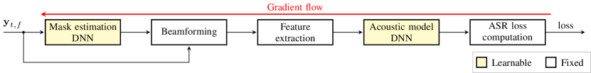
Figure 8: Schematic diagram of the joint training of the speech enhancement front-end and ASR back-end.

IV-B4 Joint-training

The above adaptation technique only adjusts the AM of the ASR back-end to the speech enhancement front-end. However, the speech enhancement front-end is usually optimized for a criterion that is not directly related to ASR. Recent works have explored a tighter integration of the speech enhancement front-end and ASR back-end, enabling optimization of the front-end for the ASR criterion [59, 132, 133]. This is relatively easy to realize because both the front-end and the back-end use neural networks, and therefore it is possible to combine them into a single neural network with learnable and fixed computational nodes. Both systems can then be jointly optimized with backpropagation as,

$$\boldsymbol{\mathbf{\hat{\theta}}}=\operatorname*{argmax}_{\boldsymbol{\mathbf{\theta}}}\sum_{u}\mathcal{C}\left(\boldsymbol{\mathbf{g}}\!\left(\text{Feat}\!\left(\text{Enh}(\mathcal{Y}_{u};\boldsymbol{\mathbf{\theta}}^{\text{enh}})\!\right);\boldsymbol{\mathbf{\theta}}^{\text{am}}\!\right),\boldsymbol{\mathbf{v}}_{u}\!\right),$$ (36)

where $\text{Enh}(\cdot)$ represents the processing of the enhancement front-end, $\mathcal{Y}_{u}$ represents the multi-channel STFT coefficients for a training utterance, and $\boldsymbol{\mathbf{\theta}}=\{\boldsymbol{\mathbf{\theta}}^{\text{am}},\boldsymbol{\mathbf{\theta}}^{\text{enh}}\}$ are the model parameters of the AM and front-end, respectively.

Fig. 8 shows an example of a joint-training scheme that combines a beamforming based front-end with the AM of the ASR back-end [59, 132, 133]. The mask estimation DNN of the front-end and the DNN of the AM are the learnable components of the system. They are interconnected with fixed computational blocks that consist of the beamformer computation (see Sec. III-B) and the feature extraction (see Sec. IV-A1). The gradient can flow from the AM to the speech enhancement front-end, which enables optimization of the front-end for ASR.

We have discussed the joint-training scheme with a beamforming front-end, but joint training has also been used for dereverberation[57] and source separation/extraction[77]. Significant ASR gains have been reported on several tasks with joint training schemes. However, joint-training can sometimes lead to a performance drop because it may weaken the AM [133].

One advantage of joint-training is that the whole system can be optimized using only far-field speech and the associated word transcriptions. Therefore, it alleviates the need for parallel clean and far-field speech data to train the speech enhancement front-end, which may be an advantage when training or adapting systems with real recordings.

V Toward Far-Field End-to-End ASR

This section describes the recent efforts towards end-to-end solutions which allow to optimize all components of the front-end speech enhancement and back-end speech recognizer jointly. This optimization is performed with respect to our final objective, the Bayes decision rule, as introduced in Eq. (25).

V-A End-to-End ASR

End-to-end ASR approaches directly model the output distribution $p(\boldsymbol{\mathbf{v}}|\boldsymbol{\mathbf{O}})$ over the character, subword, or word sequence $\boldsymbol{\mathbf{v}}=(v_{1},\dots,v_{J})$, given the speech feature sequence $\boldsymbol{\mathbf{O}}=(\boldsymbol{\mathbf{o}}_{1},\dots,\boldsymbol{\mathbf{o}}_{T})$. This is quite different from conventional approaches to ASR [92] composed of the acoustic model $p(\boldsymbol{\mathbf{O}}|\boldsymbol{\mathbf{v}})$ and language model $p(\boldsymbol{\mathbf{v}})$, as we discussed in IV-A. End-to-end models subsume all of these components in a single neural network, which greatly simplifies the model building process and also enables joint training of the whole system. The end-to-end neural speech processing has become a popular alternative to conventional ASR, and several approaches have been proposed including CTC [94], attention-based encoder-decoder models [134, 135], and their variants [136, 137].

For example, attention-based methods start from the Bayes decision theory, similar to Section IV, but do not use any conditional independence assumption, and simply factorize the posterior probability $p(\boldsymbol{\mathbf{v}}|\boldsymbol{\mathbf{O}})$ based on the probabilistic chain rule and the attention mechanism, as follows:

$$p(\boldsymbol{\mathbf{v}}|\boldsymbol{\mathbf{O}}) =\prod_{j}p(v_{j}|\boldsymbol{\mathbf{v}}_{1:j-1},\boldsymbol{\mathbf{O}})$$

$$=\prod_{j}p(v_{j}|\boldsymbol{\mathbf{v}}_{1:j-1},\boldsymbol{\mathbf{c}}_{j};\boldsymbol{\mathbf{\theta}}^{\text{dec}}),$$ (37)

where $\boldsymbol{\mathbf{v}}_{1:j-1}=(v_{1},\dots,v_{j-1})$ is a subsequence of $\boldsymbol{\mathbf{v}}$ representing the word history before word $v_{j}$. $\boldsymbol{\mathbf{c}}_{j}$ is called a context vector obtained at each token position $j$, and is extracted from the input speech feature $\boldsymbol{\mathbf{O}}$ based on the attention mechanism, which we will explain below. $p(v_{j}|\boldsymbol{\mathbf{v}}_{1:j-1},\boldsymbol{\mathbf{c}}_{j};\boldsymbol{\mathbf{\theta}}^{\text{dec}})$ is computed with a neural network called a decoder network with its set of model parameters $\boldsymbol{\mathbf{\theta}}^{\text{dec}}$, which can generate a token sequence $v_{j}$ given the history $\boldsymbol{\mathbf{v}}_{1:j-1}$ and a context vector $\boldsymbol{\mathbf{c}}_{j}$. The decoder network is often represented as an LSTM model with hidden state vector $\boldsymbol{\mathbf{z}}_{j}$ for each token position $j$.

To obtain context vector $\boldsymbol{\mathbf{c}}_{j}$ in Eq. (37), we first focus on an input feature conversion based on an encoder network. The encoder network takes the original speech feature sequence $\boldsymbol{\mathbf{O}}$ as input and converts it to high-level hidden vector sequence $\boldsymbol{\mathbf{O}}^{\text{enc}}=(\boldsymbol{\mathbf{o}}_{1}^{\text{enc}},\dots,\boldsymbol{\mathbf{o}}_{T^{\prime}}^{\text{enc}})$, as follows:

$$\boldsymbol{\mathbf{O}}^{\text{enc}}=\text{Enc}(\boldsymbol{\mathbf{O}};\boldsymbol{\mathbf{\theta}}^{\text{enc}}),$$ (38)

where $\boldsymbol{\mathbf{\theta}}^{\text{enc}}$ is a set of model parameters in the encoder network.

We often use bi-directional LSTM (BLSTM) or self-attention models as an encoder network.

Given $\boldsymbol{\mathbf{O}}^{\text{enc}}$, an attention mechanism produces context vector $\boldsymbol{\mathbf{c}}_{j}$ for each token $v_{j}$ as follows [134]:

$$\boldsymbol{\mathbf{c}}_{j}=\text{Att}\left(\boldsymbol{\mathbf{O}}^{\text{enc}},\boldsymbol{\mathbf{z}}_{j-1};\boldsymbol{\mathbf{\theta}}^{\text{att}}\right),$$ (39)

where $\boldsymbol{\mathbf{z}}_{j-1}$ is a hidden state vector introduced in the decoder network. $\text{Att}(\cdot)$ is an attention network with a set of model parameters $\boldsymbol{\mathbf{\theta}}^{\text{att}}$, which first computes the attention weight $\zeta_{jt}\in[0,1]$ given the encoder output vector $\boldsymbol{\mathbf{o}}_{t}^{\text{enc}}$ and the decoder hidden vector $\boldsymbol{\mathbf{z}}_{j-1}$ obtained in the previous output time step [134], as follows:

$$\zeta_{jt}=f^{\text{att}}(\boldsymbol{\mathbf{o}}_{t}^{\text{enc}},\boldsymbol{\mathbf{z}}_{j-1}),$$ (40)

where $f^{\text{att}}(\cdot)$ is a function to produce the attention weight, which can be a dot product or neural network-based operations with trainable parameters. $\zeta_{jt}$ satisfies the sum-to-one condition across the input frames, i.e., $\sum_{t=1}^{T^{\prime}}\zeta_{jt}=1$. Given the attention weight $\zeta_{jt}$ in Eq. (40), the context vector $\boldsymbol{\mathbf{c}}_{j}$ is obtained as a weighted summation of encoder output sequence $\boldsymbol{\mathbf{O}}^{\text{enc}}$, i.e.,

$$\boldsymbol{\mathbf{c}}_{j}=\sum_{t=1}^{T^{\prime}}\zeta_{jt}\boldsymbol{\mathbf{o}}_{t}^{\text{enc}}.$$ (41)

Note that Eq. (41) can perform a conversion between two values with different time scales (input time $t$ and output time $j$) through the soft alignment based on the weighted summation. For example, Fig. 9 depicts the attention mechanism based on Eq. (41). The bold lines correspond to the higher attention weights and the attention mechanism obtains the soft alignment between these input and output vectors. This is different from the alignment process in conventional ASR, which is based on HMMs, as discussed in Section IV-A2.

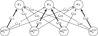
Figure 9: The attention mechanism to compute the alignment between input encoder vector $\boldsymbol{\mathbf{o}}_{t}^{\text{enc}}$ at frame $t$ and output context vector $\boldsymbol{\mathbf{c}}_{j}$ at token $j$. $\zeta_{jt}$ denotes the attention weight. The bold lines correspond to the higher attention weights and the attention mechanism obtains the soft alignment between these input and output vectors.

The forward computation of the attention-based end-to-end ASR is processed as follows:

1. Encoder processing: $\boldsymbol{\mathbf{O}}^{\text{enc}}=\text{Enc}(\boldsymbol{\mathbf{O}};\boldsymbol{\mathbf{\theta}}^{\text{enc}})$

2. For each $j$

   1. compute $\boldsymbol{\mathbf{c}}_{j}=\text{Att}(\boldsymbol{\mathbf{O}}^{\text{enc}},\boldsymbol{\mathbf{z}}_{j-1};\boldsymbol{\mathbf{\theta}}^{\text{att}})$

   2. obtain $p(v_{j}|\boldsymbol{\mathbf{v}}_{1:j-1},\boldsymbol{\mathbf{c}}_{j};\boldsymbol{\mathbf{\theta}}^{\text{dec}})$.

Figure 10 shows an entire encoder-decoder neural network with an attention mechanism. Note that the history subsequence $\boldsymbol{\mathbf{v}}_{1:j-1}$ can be obtained from the reference transcription during training and from prediction results during decoding. All of these steps are differentiable, and we can estimate the model parameters $\boldsymbol{\mathbf{\theta}}=\{\boldsymbol{\mathbf{\theta}}^{\text{enc}},\boldsymbol{\mathbf{\theta}}^{\text{att}},\boldsymbol{\mathbf{\theta}}^{\text{dec}}\}$ by maximizing the following log-likelihood, similar to Eq. (30),

$$\boldsymbol{\mathbf{\hat{\theta}}}=\operatorname*{argmax}_{\boldsymbol{\mathbf{\theta}}}\sum_{u}\log(p(\boldsymbol{\mathbf{v}}_{u}|\boldsymbol{\mathbf{O}}_{u};\boldsymbol{\mathbf{\theta}})).$$ (42)

Thus, the attention-based encoder decoder network represents an entire ASR process with a single neural network, and can be trained in an end-to-end manner unlike the conventional HMM-based ASR system. Alternatively, a transformer architecture, which is originally proposed in neural machine translation [99] to replace RNNs with self-attention networks, has been used as a variant of attention based methods for ASR [100].

Figure 10: Attention-based encoder decoder network. The attention is controlled by the decoder LSTM state.

V-B Multi-Channel End-to-End ASR

The straightforward extension of this methodology to far-field speech recognition is to combine all speech enhancement modules and ASR with a single neural network to enable joint optimization [138, 139]. This method can be regarded as an extension of the joint-training methods [59, 132, 133] of multi-channel speech enhancement and acoustic modeling as discussed in Section IV-B4.

By following Eq. (37), multi-channel end-to-end ASR directly models the posterior distribution $p(\boldsymbol{\mathbf{v}}|\mathcal{Y})$, given the sequence of multi-channel (STFT) signals $\mathcal{Y}=([\boldsymbol{\mathbf{y}}_{1,1}^{\mathrm{T}},\dots,\boldsymbol{\mathbf{y}}_{1,F}^{\mathrm{T}}],\dots,[\boldsymbol{\mathbf{y}}_{t,1}^{\mathrm{T}},\dots,\boldsymbol{\mathbf{y}}_{t,F}^{\mathrm{T}}],\dots)$:

$$p(\boldsymbol{\mathbf{v}}|\mathcal{Y}) =\prod_{j}p(v_{j}|\boldsymbol{\mathbf{v}}_{1:j-1},\mathcal{Y})=\prod_{j}p(v_{j}|\boldsymbol{\mathbf{v}}_{1:j-1},\hat{\boldsymbol{\mathbf{O}}}),$$ (43)

where

$$\hat{\boldsymbol{\mathbf{O}}}=\text{Feat}(\text{Enh}(\mathcal{Y};\theta^{\text{enh}})).$$ (44)

$\text{Enh}(\cdot)$ corresponds to the multi-channel enhancement with a set of parameters $\theta^{\text{enh}}$ and $\text{Feat }(\cdot)$ denotes the standard speech feature extraction to produce an enhanced speech feature sequence, $\hat{\boldsymbol{\mathbf{O}}}$. Both are introduced in the joint training of speech enhancement and recognition in Eq. (36).

As an instance of the multi-channel enhancement function, [138] uses BLSTM mask-based beamforming [18, 75], as described in Section III. This model is trained with an end-to-end ASR objective (cross entropy given the reference transcriptions $\boldsymbol{\mathbf{v}}_{u}$ for utterance $u$) as follows:

$$\boldsymbol{\mathbf{\hat{\theta}}}=\operatorname*{argmax}_{\boldsymbol{\mathbf{\theta}}}\sum_{u}\log(p(\boldsymbol{\mathbf{v}}_{u}|\mathcal{Y}_{u};\boldsymbol{\mathbf{\theta}})),$$ (45)

where the model parameters $\boldsymbol{\mathbf{\theta}}$ consist of the parameters of the enhancement, encoder, attention and decoder networks as,

$$\boldsymbol{\mathbf{\theta}}=\{\boldsymbol{\mathbf{\theta}}^{\text{enh}},\boldsymbol{\mathbf{\theta}}^{\text{enc}},\boldsymbol{\mathbf{\theta}}^{\text{att}},\boldsymbol{\mathbf{\theta}}^{\text{dec}}\}.$$ (46)

Compared with the standard end-to-end ASR training in Eq. (42), the multi-channel extension can jointly estimate both ASR model parameters and the enhancement parameters $\boldsymbol{\mathbf{\theta}}^{\text{enh}}$ in an end-to-end manner. Note that this model can be trained without requiring any parallel data (pairs of clean and noisy speech data), as described in Section III or any other intermediate HMM state/phoneme alignments compared with standard acoustic model training described in Eq. (34). End-to-end joint training thus allows training the enhancement parameters with real far-field data, for which clean reference signals are usually not available. The only requirement is the availability of the transcription of the far-field data, which is always required for ASR training based on supervised learning.

There are several variants and extensions of multi-channel end-to-end ASR including

• Attention-based channel/array selection [140, 141]

• Incorporation of a dereverberation component [142]

• Extension to multispeaker ASR [143]

• Extension to target speech extraction [144, 145].

Although end-to-end approaches are promising, they do not reach the performance of current state-of-the-art far-field ASR systems. The main reason is that these solutions tend to require larger amounts of training data, which, in the case of multi-channel far-field recordings, may not always be available. However, there has been a lot of progress in end-to-end ASR including extensive investigations of training methods and architectures [146, 147], robust training based on data augmentation [119], and new architectures based on the transformer model [148, 100].

VI Summary and remaining challenges

VI-A Summary

This paper emphasizes that multi-channel speech enhancement is an essential component for far-field ASR, and provides a comprehensive description of state-of-the-art enhancement techniques in Section III. The combination of powerful signal processing with deep learning significantly boosted the performance, compared to earlier signal processing-only solutions. This trend of solving a problem with signal processing supported by a neural network is not so often seen in other applications of deep learning. Consider, for example, computer vision, where an entire signal processing pipeline has been replaced with a very deep network. The main reason of this unique approach in speech enhancement is that well-established physical models exist, which can be viewed as regularizers when devising a deep learning solution. We can thus minimize the size of the neural networks and can make multi-channel speech enhancement work robustly with a relatively small amount of training data.

The main focus of the description of the back-end ASR system in Section IV is on how to make use of deep learning techniques in ASR acoustic models for the far-field ASR scenario. This includes techniques like data augmentation, refinement of supervisions, and adaptation. Note that, unlike speech enhancement, ASR is not based on a solid physical model describing human speech perception and recognition, while at the same time single-channel data in the order of thousands of hours have become available also in an academic research setting. This is why pure deep learning based solutions excel at ASR. Overall, the fusion of neural network-supported signal processing in the front-end and the massive use of deep learning in the back-end has made far-field ASR so reliable that it entered the consumer market with products like digital home assistants.

This paper also introduced the new research paradigm of jointly modeling front-end speech enhancement and back-end ASR acoustic models in Section IV-B4. Section V further extended this joint training scheme towards the emergent end-to-end ASR framework. The underlying idea of both approaches is to strictly follow the above established far-field ASR pipeline, but to represent it with a single neural network so that we can perform back propagation to train both speech enhancement and recognition jointly. Currently, joint training and end-to-end approaches have not yet become as mainstream as the pipeline approach due to their complex network architecture and the lack of a sufficient amount of multi-channel far-field training data. However, we believe that these approaches have a lot of potential to provide further breakthroughs in far-field ASR, and we put emphasis on describing them as our most important on-going and future research directions.

VI-B Remaining challenges

The following subsections list remaining challenges in far-field ASR. For some of those, including voice activity detection and speaker diarization, there exist well-established solutions in a clean speech environment, while they remain to be challenging in far-field ASR conditions.

• Voice Activity Detection (VAD) (also called Speech Activity Detection (SAD)) is an essential technique to segment continuous audio signals in on-line streaming ASR, or long audio recordings in off-line ASR into utterances of manageable length (up to, say, a dozen seconds). Traditionally, energy-based VAD or likelihood based solutions [149] have been used. However, these methods face significant degradation in low SNR conditions. Learning based methods, especially RNN-based ones, combined with data augmentation techniques as described in Section IV-B1 have become popular [150, 151], because they can detect speech activity regions by non-linear feature mapping even in the presence of low SNR. There are also several challenge activities including OpenSAD. Further note that VAD-related challenge activities are also included in the speaker diarization challenge, see next item.

• Speaker diarization: Speaker diarization can be regarded as an extension of VAD to multi-speaker recordings, which provides speaker identities or speaker cluster assignments for each utterance from unsegmented audio signals, i.e., it provides information about “who speaks when” [152]. Recently, speaker diarization has received increased attention because the focus of the ASR research community is shifting more and more towards recognition of multi-speaker recordings such as conversations or meetings, The interest in diarization is boosted by several challenge activities including DIHARD and CHiME-6. There are two main technologies depending on whether single-channel or multi-channel data is available. When we have multi-channel audio signals, source speaker locations can be estimated based on beamforming, and this can in turn be exploited to provide diarization information [153, 152]. In the single-channel case, people use speaker embeddings, such as the i-vector [154] or x-vector [155], to map a speech utterance into a fixed dimensional vector, and then perform clustering on those obtained embedding vectors (e.g., agglomerative hierarchical clustering (AHC) [156, 157]). VAD is used as an initial module in the speaker diarization pipeline to segment the recordings into manageable utterances. However, most single-channel techniques cannot explicitly handle regions of speech, where more than one speaker is active. But such overlap regions are common in real conversations [4]. A combination of speech separation, speaker counting, and diarization based on neural networks [158] and permutation-free neural diarization based on multiple label classification [159] would be a promising direction to tackle regions of overlapped speech.

• On-line processing: Another challenge of far-field speech processing is on-line, low-latency processing which is mandatory when used in a spoken language interface. It also has some benefits in dynamical environments, when, e.g., moving sources have to be tracked, see the next bullet in this list. Speech enhancement techniques often require to estimate signal statistics across frames, such as the spatial covariance matrix $\boldsymbol{\mathbf{\Phi}}$ for beamforming used in Eq. (20) and the MCLP coefficient matrix $\boldsymbol{\mathbf{C}}$ for dereverberation, Eqs. (12) and (13). If low latency is required, this statistics computation must be performed in an on-line manner, often based on recursive update equations, e.g., by a linear interpolation between previously estimated statistics and the current observations. Online processing for mask-based beamforming is discussed in [160, 161]. [95] gives an overview of the development of the Google Home device and describes several online techniques [47], especially for dereverberation. [56, 58] realizes online WPE dereverberation with the help of DNN-based time varying variance estimation.

• Dynamic environments: moving sensors and sources: Acoustic environments are changing over time due to nonstationary noise, moving sources or moving sensors. For example, the participants recorded in the CHiME-5 data set are moving from room to room [4], and front-end processing has to track such moving sources accordingly. In addition, with wearable microphones and in moving robot scenarios [162], we should also take moving microphones into consideration. In these situations, on-line processing as discussed above is necessary to deal with adaptive estimation of enhancement filters (beamforming, dereverberation). Recently, there has been a challenge activity, the LOCATA Challenge[163], on locating and tracking moving sources. Although this challenge mainly focuses on acoustic source localization and not on speech enhancement and recognition, their designs of dynamic environments and the defined evaluation metrics for source tracking would be a good reference for tackling far-field speech recognition in dynamic environments.

• More natural conversations and spontaneous speech. Our conversations are often spontaneous, and speech characteristics are quite variable and complex. For example, in the dinner party scenarios of CHiME 5 [4] and the Santa Barbara corpus [164], we often observe very different speaking durations, volumes, and speaking styles during the conversation. Such variable speech characteristics make the statistical properties of source signals complex and renders estimation of speech statistics harder. In addition, the spoken contents are grammatically less regular due to filler words, mispronunciation, stammering, etc., which makes ASR quite challenging from both acoustic and language model perspectives. Finally, such conversations are challenging in terms of the data collection and annotation perspectives, because the preparation of precise transcriptions is difficult.

• Improving signal extraction with semantic and syntactic context information: A human’s ability to track a conversation in acoustically adverse conditions (e.g., in a cocktail party) can in part be attributed to the use of context information about the discussion topic, our “world knowledge” and syntactic constraints we are aware of. Only few works exist towards utilizing high-level guidance for the low-level signal extraction tasks. In [165] the speech separation is improved by feeding back deep features extracted from an end-to-end ASR system to cover the long-term dependence of phonetic aspects, while sound separation is improved in [166] by utilizing sound classification results. Exploring ways to support front-end processing with back-end knowledge appears to be a promising way to improve overall system performance.

• Distributed microphone setup: In many application scenarios, including smart homes [4, 167], wearable computing, and human-to-robot communication [162], distributed microphones can be of an advantage, compared to a single spatially concentrated microphone array. However, the challenge of distributed microphones is that their spatial location is often a priori unknown and may change over time. Furthermore, the microphone characteristics can be different, e.g., if both mobile phones and desktop microphones are part of the network. Finally, and most importantly, the sampling rates of the microphones are not synchronized in general. These properties often break important assumptions made in conventional front-end processing, and thus standard beamforming and dereverberation techniques cannot be straightforwardly applied. However, there exist several studies to tackle the distributed microphone setup including [168, 169, 170, 171, 172] by solving the synchronization problem to make beamforming work in this setup. There are also many works on distributed beamforming, e.g., [173, 174, 175], to avoid collecting all signals at a central processing node. Active microphone (subset) selection instead of fusing the signals of multiple microphones is another simple yet effective approach [176, 177]. Also, late fusion techniques (acoustic model fusion [103] or hypothesis fusion [107] in ASR) instead of signal-level fusion can be a viable alternative thanks to the relative insensitivity of acoustic models to synchronization errors.

• Multimodality: A final challenges in far-field speech recognition is the use of multimodal information including videos, accelerometer, biosignals and so on. Such information would be complementary to audio signals, be robust against acoustic noise, and thus the fusion can bring benefits. In particular, audio-visual speech recognition gains a lot of attention as the video channel can provide the speaker location information for steering an acoustic beamformer. Furthermore, visual features can complement the audio features for noise robust speech recognition [178]. However, the visual or other multimodal data have their own distortions (e.g., brightness and frame-out issues of the image), and synchronization across different modalities is also another challenge.

VII To probe further

Open-source implementations are available for most of the described techniques and provide a good starting point for a more hands-on experience.

A Python implementation of the WPE algorithm described in Sec. III-A based on Numpy and Tensorflow is provided by NaraWPE [179]. The Matlab implementation originally used in [21, 46] is available as pcode. For beamforming as described in Sec. III-B, two different Python implementations are provided. NN-GEV focuses on neural network-based mask estimation and subsequent beamforming while PB-BSS focuses on spatial clustering-based Speech Presense Probability (SPP) estimation. Other useful toolkits implementing dereverberation and beamforming techniques include the BTK toolkit and Pyroomacoustics [180]. The latter one also allows to simulate acoustic scenarios to generate data.

An overview of selected implementations is given in Table II while databases are listed in Table I. To visualize the comprehension of the effect of far-field speech and prospective improvements for several acoustic scenarios, Fig. 11 depicts the ASR performance transition of the CHiME and REVERB challenges from the challenge baseline at the challenge release period, the challenge best system, and the challenge follow up studies. By referring to Fig. 11 and corresponding acoustic scenarios in Table I., we can monitor the prospective improvement of various far-field ASR problems.

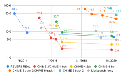
Figure 11: The WER transitions of far-field ASR systems based on the REVERB and CHiME-3/4/5/6 challenge results from their baseline systems, challenge best systems, and the follow-up studies.

Note that many of these ASR results can be reproduced by using publicly available toolkits. For a head-start on ASR tasks, the Kaldi toolkit [181] provides several recipes for the listed databases which include some of the tools discussed above. The CHiME-6 recipe for example uses NaraWPE and PB-GSS while the CHiME-3/4 recipe includes BeamformIt and NN-GEV. ESPnet [182] also provides multichannel end-to-end ASR for the REVERB and CHiME-4 data with the help of DNN-WPE.

TABLE I: Recent noise robust speech recognition tasks.

Task	​​Vocabulary​​ size	Amount of training data	Realism	Type of distortions	Number of mics	Mic-speaker distance	Ground truth
ASpIRE [6]	100k	N/A	Real	Reverberation	8/1	N/A	N/A
AMI [183]	11k	$\sim$ 107k utt. ($\sim$ 75 h)	Real	Multi-speaker conversations Reverberation and noise	8	N/A	Headset
CHiME-3/4 [2, 3]	5k	8738 utt. ($\sim$ $18\text{\,}\mathrm{h}$)	Simu+Real	Nonstationary noise in four public environments	6/2/1	$0.5\text{\,}\mathrm{m}$	Clean/ close talk
CHiME-5/6 [4]	100k	$\sim$ 80k utt. ($\sim$ $40\text{\,}\mathrm{h}$)	Real	Nonstationary noise, multi-speaker conversations, reverberation	32	$0.5\text{\,}\mathrm{m}$ to $2\text{\,}\mathrm{m}$	Binaural headset
REVERB [1]	5k	7861 utt. ($\sim$ $15\text{\,}\mathrm{h}$)	Simu+Real	Reverberation in different living rooms	8/2/1	$0.5\text{\,}\mathrm{m}$ to $2\text{\,}\mathrm{m}$	Clean/ headset

TABLE II: Toolkits

Name	Affiliation	Function	Interface	Back-end	License	Ref.
NaraWPE	UPB	WPE dereverberation	Python	NumPy, TensorFlow​​​​	MIT	[179]
WPE	NTT	WPE dereverberation	Matlab	Matlab	Custom	[21, 46]
DNN-WPE	NTT	DNN-based WPE dereverberation​​	Python	NumPy, PyTorch	Custom	[56]
NN-GEV	UPB	Neural mask-based beamforming	Python	NumPy, Chainer	Custom	[74]
PB-BSS	UPB	Spatial clustering, beamforming	Python	NumPy	MIT	[55]
BTK	CMU	Beamforming, dereverberation	Python, C++	C++	MIT	N/A
PyRoomAcoustics​​​​​​​​	EPFL	Beamforming, RIR generation	Python	NumPy/C	MIT	[180]
BeamformIt	ICSI	Delay-and-sum beamforming	CLI, C++	C/C++	N/A	[184]
HARK	HRI	Source localization, separation	CLI, Python	C++	Custom	hark.jp

References

- [1] K. Kinoshita, M. Delcroix, S. Gannot, E. Habets, R. Haeb-Umbach, W. Kellermann, V. Leutnant, R. Maas, T. Nakatani, B. Raj, A. Sehr, and T. Yoshioka, “A summary of the REVERB challenge: state-of-the-art and remaining challenges in reverberant speech processing research,” EURASIP Journal on Advances in Signal Processing, 2016.
- [2] J. Barker, R. Marxer, E. Vincent, and S. Watanabe, “The third ”CHiME” speech separation and recognition challenge: Analysis and outcomes,” Computer Speech and Language, vol. 46, pp. 605–626, Nov. 2017.
- [3] E. Vincent, S. Watanabe, A. A. Nugraha, J. Barker, and R. Marxer, “An analysis of environment, microphone and data simulation mismatches in robust speech recognition,” Computer Speech and Language, 2016.
- [4] J. Barker, S. Watanabe, E. Vincent, and J. Trmal, “The fifth ’CHiME’ speech separation and recognition challenge: Dataset, task and baselines,” in Proc. of Annual Conference of the International Speech Communication Association (Interspeech), 2018.
- [5] S. Watanabe, M. Mandel, J. Barker, E. Vincent, A. Arora, X. Chang, S. Khudanpur, V. Manohar, D. Povey, D. Raj, D. Snyder, A. S. Subramanian, J. Trmal, B. B. Yair, C. Boeddeker, Z. Ni, Y. Fujita, S. Horiguchi, N. Kanda, T. Yoshioka, and N. Ryant, “CHiME-6 challenge: Tackling multispeaker speech recognition for unsegmented recordings,” CoRR, 2020.
- [6] M. Harper, “The automatic speech recogition in reverberant environments (ASpIRE) challenge,” in Proc. of IEEE Workshop on Automatic Speech Recognition and Understanding (ASRU), Dec 2015, pp. 547–554.
- [7] M. Delcroix, T. Yoshioka, A. Ogawa, Y. Kubo, M. Fujimoto, N. Ito, K. Kinoshita, M. Espi, S. Araki, T. Hori et al., “Strategies for distant speech recognition in reverberant environments,” EURASIP Journal on Advances in Signal Processing, vol. 2015, no. 1, p. 60, 2015.
- [8] X. Feng, K. Kumatani, and J. McDonough, “The CMU-MIT REVERB challenge 2014 system: description and results,” in REVERB Challenge Workshop, 2014.
- [9] F. Weninger, S. Watanabe, J. L. Roux, J. R. Hershey, Y. Tachioka, and G. Rigoll, “The MERL/MELCO/TUM system for the REVERB challenge using deep recurrent neural network feature enhancement,” in REVERB Challenge Workshop, 2014.
- [10] Z.-Q. Wang and D. Wang, “Deep learning based target cancellation for speech dereverberation,” IEEE Transactions on Audio, Speech, and Language Processing, vol. 28, pp. 941–950, 2020.
- [11] J.Barker, R. Marxer, E. Vincent, and S. Watanabe, “Multi-microphone speech recognition in everyday environments,” Computer Speech and Language, vol. 46, pp. 386–387, June 2017.
- [12] S.-J. Chen, A. S. Subramanian, H. Xu, and S. Watanabe, “Building state-of-the-art distant speech recognition using the CHiME-4 challenge with a setup of speech enhancement baseline,” in Proc. of Annual Conference of the International Speech Communication Association (Interspeech), 2018, pp. 1571–1575.
- [13] C. Zorilă, C. Boeddeker, R. Doddipatla, and R. Haeb-Umbach, “An investigation into the effectiveness of enhancement in ASR training and test for CHiME-5 dinner party transcription,” in Proc. of IEEE Workshop on Automatic Speech Recognition and Understanding (ASRU), 2019.
- [14] J. Du, Y.-H. Tu, L. Sun, L. Chai, X. Tang, M.-K. He, F. Ma, J. Pan, J.-Q. Gao, D. Liu, C.-H. Lee, and J.-D. Chen, “The USTC-NELSLIP systems for CHiME-6 challenge,” in 6th CHiME Speech Separation and Recognition Challenge (CHiME-6), 2020.
- [15] G. Hinton, L. Deng, D. Yu, G. E. Dahl, A. r. Mohamed, N. Jaitly, A. Senior, V. Vanhoucke, P. Nguyen, T. N. Sainath, and B. Kingsbury, “Deep neural networks for acoustic modeling in speech recognition: The shared views of four research groups,” IEEE Signal Processing Magazine, vol. 29, no. 6, pp. 82–97, Nov 2012.
- [16] D. Yu and L. Deng, Automatic Speech Recognition – A Deep Learning Approach. Springer, 2015.
- [17] J. Li, L. Deng, R. Haeb-Umbach, and Y. Gong, Robust Automatic Speech Recognition. Elsevier, Oct 2015.
- [18] M. Souden, J. Benesty, and S. Affes, “On optimal frequency-domain multichannel linear filtering for noise reduction,” IEEE Transactions on Audio, Speech, and Language Processing, vol. 18, no. 2, pp. 260–276, 2010.
- [19] D. Van Compernolle, W. Ma, F. Xie, and M. Van Diest, “Speech recognition in noisy environments with the aid of microphone arrays,” Speech Communication, vol. 9, no. 5-6, pp. 433–442, 1990.
- [20] P. Naylor and N. Gaubitch, Eds., Speech Dereverberation. Springer, 2010.
- [21] T. Nakatani, T. Yoshioka, K. Kinoshita, M. Miyoshi, and B.-H. Juang, “Speech dereverberation based on variance-normalized delayed linear prediction,” IEEE Transactions on Audio, Speech, and Language Processing, vol. 18, no. 7, pp. 1717–1731, 2010.
- [22] S. Araki, M. Okada, T. Higuchi, A. Ogawa, and T. Nakatani, “Spatial correlation model based observation vector clustering and MVDR beamforming for meeting recognition,” in Proc. of IEEE International Conference on Acoustics, Speech and Signal Processing (ICASSP). IEEE, 2016, pp. 385–389.
- [23] B. Wu, K. Li, M. Yang, C.-H. Lee, B. Wu, K. Li, M. Yang, C.-H. Lee, B. Wu, M. Yang, C.-H. Lee, and K. Li, “A reverberation-time-aware approach to speech dereverberation based on deep neural networks,” IEEE Transactions on Audio, Speech, and Language Processing, vol. 25, no. 1, pp. 102–111, Jan. 2017.
- [24] J. R. Hershey, Z. Chen, J. Le Roux, and S. Watanabe, “Deep clustering: discriminative embeddings for segmentation and separation,” in Proc. of IEEE International Conference on Acoustics, Speech and Signal Processing (ICASSP). IEEE, 2016, pp. 31–35.
- [25] Z. Chen, Y. Luo, and N. Mesgarani, “Deep attractor network for single-microphone speaker separation,” in Proc. of IEEE International Conference on Acoustics, Speech and Signal Processing (ICASSP), March 2017, pp. 246–250.
- [26] M. Kolbæk, D. Yu, Z.-H. Tan, and J. Jensen, “Multitalker speech separation with utterance-level permutation invariant training of deep recurrent neural networks,” IEEE/ACM Transactions on Audio, Speech, and Language Processing, vol. 25, no. 10, pp. 1901–1913, 2017.
- [27] Y. Luo and N. Mesgarani, “Conv-TasNet: Surpassing ideal time-frequency magnitude masking for speech separation,” IEEE/ACM Transactions on Audio, Speech, and Language Processing, vol. PP, pp. 1–1, May 2019.
- [28] Y. Avargel and I. Cohen, “On multiplicative transfer function approximation in the short-time fourier transform domain,” IEEE Signal Processing Letters, vol. 14, pp. 337–340, 2007.
- [29] A. Gilloire and M. Vetterli, “Adaptive filtering in sub-bands with critical sampling: analysis, experiments, and application to acoustic echo cancellation,” IEEE Transactions on Signal Processing, vol. 40, no. 8, pp. 1862–1875, 1992.
- [30] R. Talmon, I. Cohen, and S. Gannot, “Convolutive transfer function generalized sidelobe canceler,” IEEE Transactions on Audio, Speech, and Language Processing, vol. 17, no. 7, pp. 1420–1434, 2009.
- [31] X. Li, L. Girin, S. Gannot, and R. Horaud, “Multichannel speech separation and enhancement using the convolutive transfer function,” IEEE/ACM Transactions on Audio, Speech, and Language Processing, vol. 27, no. 3, pp. 645–659, 2019.
- [32] “ITU-T recommendation p.862: Perceptual evaluation of speech quality (PESQ): An objective method for end-to-end speech quality assessment of narrow-band telephone networks and speech codecs,” http://www.itu.int/rec/T-REC-P.862/en, 2008.
- [33] C. H. Taal, R. C. Hendriks, R. Heusdens, and J. Jensen, “A short-time objective intelligibility measure for time-frequency weighted noisy speech,” in Proc. of IEEE International Conference on Acoustics, Speech and Signal Processing (ICASSP), March 2010, pp. 4214–4217.
- [34] E. Vincent, R. Gribonval, and C. Févotte, “Performance measurement in blind audio source separation,” IEEE Transactions on Audio, Speech, and Language Processing, vol. 14, no. 4, pp. 1462–1469, 2006.
- [35] D. Wang and J. Chen, “Supervised speech separation based on deep learning: An overview,” IEEE/ACM Transactions on Audio, Speech, and Language Processing, vol. 26, no. 10, pp. 1702–1726, 2018.
- [36] H. Buchner, R. Aichner, and W. Kellermann, “TRINICON: a versatile framework for multichannel blind signal processing,” in Proc. of IEEE International Conference on Acoustics, Speech and Signal Processing (ICASSP), vol. III, 2004, pp. 889–892.
- [37] T. Nakatani and K. Kinoshita, “Maximum likelihood convolutional beamformer for simultaneous denoising and dereverberation,” in 27th European Signal Processing Conference (EUSIPCO), 2019.
- [38] D. T. M. Slock, “Blind fractionally-spaced equalization, perfectre construction filter-banks and multichannel linear prediction,” in Proc. of IEEE International Conference on Acoustics, Speech and Signal Processing (ICASSP), vol. 4, 1994, pp. 585–588.
- [39] B. D. Van Veen and K. M. Buckley, “Beamforming: A versatile approach to spatial filtering,” IEEE ASSP Magazine, vol. 5, no. 2, pp. 4–24, April 1988.
- [40] S. Gannot, E. Vincent, S. Markovich-Golan, and A. Ozerov, “A consolidated perspective on multimicrophone speech enhancement and source separation,” IEEE Transactions on Audio, Speech, and Language Processing, vol. 25, no. 4, 2017.
- [41] C. Boeddeker, T. Nakatani, K. Kinoshita, and R. Haeb-Umbach, “Jointly optimal dereverberation and beamforming,” Submitted to ICASSP, 2020. [Online]. Available: http://arxiv.org/abs/1910.13707
- [42] K. Abed-Meraim and P. Loubaton, “Prediction error method for second-order blind identification,” IEEE Transactions on Signal Processing, vol. 45, no. 3, pp. 694–705, 1997.
- [43] E. Vincent, T. Virtanen, and S. Gannot, Audio source separation and speech enhancement. John Wiley & Sons, 2018.
- [44] S. Makino, Ed., Audio Source Separation. Springer, 2018.
- [45] F. Xiong, B. T. Meyer, N. Moritz, R. Rehr, J. Anemüller, T. Gerkmann, S. Doclo, and S. Goetze, “Front-end technologies for robust asr in reverberant environments—spectral enhancement-based dereverberation and auditory modulation filterbank features,” EURASIP Journal on Advances in Signal Processing, vol. 2015, no. 1, p. 70, 2015.
- [46] T. Yoshioka and T. Nakatani, “Generalization of multi-channel linear prediction methods for blind MIMO impulse response shortening,” IEEE Transactions on Audio, Speech, and Language Processing, 2012.
- [47] J. Caroselli, I. Shafran, A. Narayanan, and R. Rose, “Adaptive multichannel dereverberation for automatic speech recognition,” in Proc. of Annual Conference of the International Speech Communication Association (Interspeech), 2017.
- [48] T. Higuchi, N. Ito, T. Yoshioka, and T. Nakatani, “Robust MVDR beamforming using time-frequency masks for online/offline asr in noise,” in Proc. of IEEE International Conference on Acoustics, Speech and Signal Processing (ICASSP), March 2016, pp. 5210–5214.
- [49] Y. Isik, J. Le Roux, Z. Chen, S. Watanabe, and J. Hershey, “Single-channel multi-speaker separation using deep clustering,” in Proc. of Annual Conference of the International Speech Communication Association (Interspeech), 2016.
- [50] L. Griffiths and C. Jim, “An alternative approach to linearly constrained adaptive beamforming,” IEEE Transactions on Antennas and Propagation, vol. 30, no. 1, pp. 27–34, January 1982.
- [51] S. Makino, T. Lee, and H. Sawada, Blind speech separation. Springer, 2007, vol. 615.
- [52] G. Naik and W. Wang, Eds., Blind Source Separation. Springer, 2014.
- [53] J. Heymann, L. Drude, and R. Haeb-Umbach, “Neural network based spectral mask estimation for acoustic beamforming,” in Proc. of IEEE International Conference on Acoustics, Speech and Signal Processing (ICASSP), 2016.
- [54] X. Xiao, S. Watanabe, H. Erdogan, L. Lu, J. Hershey, M. L. Seltzer, G. Chen, Y. Zhang, M. Mandel, and D. Yu, “Deep beamforming networks for multi-channel speech recognition,” in Proc. of IEEE International Conference on Acoustics, Speech and Signal Processing (ICASSP), March 2016, pp. 5745–5749.
- [55] L. Drude and R. Haeb-Umbach, “Tight integration of spatial and spectral features for BSS with deep clustering embeddings,” in Proc. of Annual Conference of the International Speech Communication Association (Interspeech), 2017.
- [56] K. Kinoshita, M. Delcroix, H. Kwon, T. Mori, and T. Nakatani, “Neural network-based spectrum estimation for online WPE dereverberation,” in Proc. of Annual Conference of the International Speech Communication Association (Interspeech), 2017, pp. 384–388.
- [57] J. Heymann, L. Drude, R. Haeb-Umbach, K. Kinoshita, and T. Nakatani, “Joint optimization of neural network-based WPE dereverberation and acoustic model for robust online ASR,” in Proc. of IEEE International Conference on Acoustics, Speech and Signal Processing (ICASSP). IEEE, 2019, pp. 6655–6659.
- [58] ——, “Frame-online DNN-WPE dereverberation,” in Proc. IWAENC, Tokyo, Japan, September 2018.
- [59] J. Heymann, L. Drude, C. Boeddeker, P. Hanebrink, and R. Haeb-Umbach, “BEAMNET: End-to-end training of a beamformer-supported multi-channel ASR system,” in Proc. of IEEE International Conference on Acoustics, Speech and Signal Processing (ICASSP), 2017.
- [60] A. Jukić, T. van Waterschoot, T. Gerkmann, and S. Doclo, “Multi-channel linear prediction-based speech dereverberation with sparse priors,” IEEE Transactions on Audio, Speech, and Language Processing, vol. 23, no. 9, pp. 1509–1520, 2015.
- [61] S. R. Chetupalli and T. V. Sreenivas, “Late reverberation cancellation using Bayesian estimation of multi-channel linear predictors and student’s t-source prior,” IEEE Transactions on Audio, Speech, and Language Processing, vol. 27, no. 6, 2019.
- [62] M. Miyoshi and Y. Kaneda, “Inverse filtering of room acoustics,” IEEE Trans. Acoustics, Speech, and Signal Processing, vol. 36, no. 2, pp. 145–152, 1988.
- [63] S. Braun, A. Kuklasiński, O. Schwartz, O. Thiergart, E. A. Habets, S. Gannot, S. Doclo, and J. Jensen, “Evaluation and comparison of late reverberation power spectral density estimators,” IEEE Transactions on Audio, Speech, and Language Processing, vol. 26, no. 6, pp. 1056–1071, 2018.
- [64] S. Gannot, D. Burshtein, and E. Weinstein, “Signal enhancement using beamforming and nonstationarity with applications to speech,” IEEE Transactions on Signal Processing, vol. 49, no. 8, pp. 1614–1626, 2001.
- [65] O. Schwartz, S. Gannot, and E. Habets, “Multi-microphone speech dereverberation and noise reduction using relative early transfer functions,” IEEE/ACM Transactions on Audio, Speech, and Language Processing, vol. 23, no. 2, pp. 240–251, 2015.
- [66] E. Warsitz, A. Krueger, and R. Haeb-Umbach, “Speech enhancement with a new generalized eigenvector blocking matrix for application in a generalized sidelobe canceller,” in Proc. of IEEE International Conference on Acoustics, Speech and Signal Processing (ICASSP), 2008, pp. 73–76.
- [67] M. I. Mandel, D. P. Ellis, and T. Jebara, “An EM algorithm for localizing multiple sound sources in reverberant environments,” in Advances in neural information processing systems, 2007, pp. 953–960.
- [68] D. H. Tran Vu and R. Haeb-Umbach, “Blind speech separation employing directional statistics in an expectation maximization framework,” in Proc. of IEEE International Conference on Acoustics, Speech and Signal Processing (ICASSP). IEEE, 2010, pp. 241–244.
- [69] N. Ito, S. Araki, and T. Nakatani, “Modeling audio directional statistics using a complex Bingham mixture model for blind source extraction from diffuse noise,” in Proc. of IEEE International Conference on Acoustics, Speech and Signal Processing (ICASSP). IEEE, 2016, pp. 465–468.
- [70] ——, “Complex angular central Gaussian mixture model for directional statistics in mask-based microphone array signal processing,” in European Signal Processing Conference (EUSIPCO). IEEE, 2016, pp. 1153–1157.
- [71] T. Yoshioka, N. Ito, M. Delcroix, A. Ogawa, K. Kinoshita, M. Fujimoto, C. Yu, W. J. Fabian, M. Espi, T. Higuchi et al., “The NTT CHiME-3 system: Advances in speech enhancement and recognition for mobile multi-microphone devices,” in Proc. of IEEE Workshop on Automatic Speech Recognition and Understanding (ASRU). IEEE, 2015, pp. 436–443.
- [72] Y. Li and D. Wang, “On the optimality of ideal binary time–frequency masks,” Speech Communication, vol. 51, no. 3, pp. 230–239, 2009.
- [73] H. Erdogan, J. R. Hershey, S. Watanabe, and J. Le Roux, “Phase-sensitive and recognition-boosted speech separation using deep recurrent neural networks,” in Proc. of IEEE International Conference on Acoustics, Speech and Signal Processing (ICASSP). IEEE, 2015.
- [74] J. Heymann, L. Drude, A. Chinaev, and R. Haeb-Umbach, “BLSTM supported GEV beamformer front-end for the 3rd CHiME challenge,” in Proc. of IEEE Workshop on Automatic Speech Recognition and Understanding (ASRU), December 2015.
- [75] H. Erdogan, J. R. Hershey, S. Watanabe, M. I. Mandel, and J. Le Roux, “Improved MVDR beamforming using single-channel mask prediction networks,” in Proc. of Annual Conference of the International Speech Communication Association (Interspeech), 2016, pp. 1981–1985.
- [76] K. Žmolíková, M. Delcroix, K. Kinoshita, T. Higuchi, A. Ogawa, and T. Nakatani, “Speaker-aware neural network based beamformer for speaker extraction in speech mixtures,” in Proc. of Annual Conference of the International Speech Communication Association (Interspeech), 2017, pp. 2655–2659.
- [77] K. Žmolíková, M. Delcroix, K. Kinoshita, T. Ochiai, T. Nakatani, L. Burget, and J. Černockỳ, “SpeakerBeam: Speaker aware neural network for target speaker extraction in speech mixtures,” IEEE Journal of Selected Topics in Signal Processing, vol. 13, no. 4, pp. 800–814, 2019.
- [78] K. Veselỳ, S. Watanabe, K. Žmolíková, M. Karafiát, L. Burget, and J. H. Černockỳ, “Sequence summarizing neural network for speaker adaptation,” in Proc. of IEEE International Conference on Acoustics, Speech and Signal Processing (ICASSP). IEEE, 2016, pp. 5315–5319.
- [79] Q. Wang, H. Muckenhirn, K. Wilson, P. Sridhar, Z. Wu, J. Hershey, R. A. Saurous, R. J. Weiss, Y. Jia, and I. L. Moreno, “Voicefilter: Targeted voice separation by speaker-conditioned spectrogram masking,” arXiv preprint arXiv:1810.04826, 2018.
- [80] C. Boeddeker, J. Heitkaemper, J. Schmalenstroeer, L. Drude, J. Heymann, and R. Haeb-Umbach, “Front-end processing for the CHiME-5 dinner party scenario,” in CHiME5 Workshop, 2018.
- [81] H. Sawada, R. Mukai, S. Araki, and S. Makino, “A robust and precise method for solving the permutation problem of frequency-domain blind source separation,” IEEE Transactions on Speech and Audio Processing, vol. 12, no. 5, pp. 530–538, 2004.
- [82] D. Yu, M. Kolbæk, Z.-H. Tan, and J. Jensen, “Permutation invariant training of deep models for speaker-independent multi-talker speech separation,” arXiv preprint arXiv:1607.00325, 2016.
- [83] L. Drude, D. Hasenklever, and R. Haeb-Umbach, “Unsupervised training of a deep clustering model for multichannel blind source separation,” in Proc. of IEEE International Conference on Acoustics, Speech and Signal Processing (ICASSP). IEEE, 2019.
- [84] P. Seetharaman, G. Wichern, J. Le Roux, and B. Pardo, “Bootstrapping single-channel source separation via unsupervised spatial clustering on stereo mixtures,” in Proc. of IEEE International Conference on Acoustics, Speech and Signal Processing (ICASSP). IEEE, 2019.
- [85] E. Tzinis, S. Venkataramani, and P. Smaragdis, “Unsupervised deep clustering for source separation: Direct learning from mixtures using spatial information,” in Proc. of IEEE International Conference on Acoustics, Speech and Signal Processing (ICASSP). IEEE, 2019.
- [86] Z.-Q. Wang, J. Le Roux, and J. R. Hershey, “Multi-channel deep clustering: Discriminative spectral and spatial embeddings for speaker-independent speech separation,” in Proc. of IEEE International Conference on Acoustics, Speech and Signal Processing (ICASSP). IEEE, 2018.
- [87] T. Nakatani, N. Ito, T. Higuchi, S. Araki, and K. Kinoshita, “Integrating DNN-based and spatial clustering-based mask estimation for robust MVDR beamforming,” in Proc. of IEEE International Conference on Acoustics, Speech and Signal Processing (ICASSP). IEEE, 2017.
- [88] L. Drude and R. Haeb-Umbach, “Integration of neural networks and probabilistic spatial models for acoustic blind source separation,” IEEE Journal of Selected Topics in Signal Processing, 2019.
- [89] L. Drude, C. Boeddeker, J. Heymann, R. Haeb-Umbach, K. Kinoshita, M. Delcroix, and T. Nakatani, “Integrating neural network based beamforming and weighted prediction error dereverberation,” in Proc. of Annual Conference of the International Speech Communication Association (Interspeech), 2018, pp. 3043–3047.
- [90] T. Yoshioka, H. Erdogan, Z. Chen, X. Xiao, and F. Alleva, “Recognizing overlapped speech in meetings: A multichannel separation approach using neural networks,” Proc. of Annual Conference of the International Speech Communication Association (Interspeech), pp. 3038–3042, 2018.
- [91] L. Rabiner and B.-H. Juang, “Historical perspective of the field of ASR/NLU,” in Springer handbook of speech processing. Springer, 2008, pp. 521–538.
- [92] L. R. Rabiner, “A tutorial on hidden Markov models and selected applications in speech recognition,” Proceedings of the IEEE, vol. 77, no. 2, pp. 257–286, 1989.
- [93] X. Huang, A. Acero, and H.-W. Hon, Spoken Language Processing: A Guide to Theory, Algorithm, and System Development, 1st ed. Upper Saddle River, NJ, USA: Prentice Hall PTR, 2001.
- [94] A. Graves, S. Fernández, F. Gomez, and J. Schmidhuber, “Connectionist temporal classification: labelling unsegmented sequence data with recurrent neural networks,” in Proc. of International Conference on Machine Learning (ICML), 2006, pp. 369–376.
- [95] B. Li, T. Sainath, A. Narayanan, J. Caroselli, M. Bacchiani, A. Misra, I. Shafran, H. Sak, G. Pundak, K. Chin, K. C. Sim, R. J. Weiss, K. Wilson, E. Variani, C. Kim, O. Siohan, M. Weintraub, E. McDermott, R. Rose, and M. Shannon, “Acoustic modeling for Google Home,” in Proc. of Annual Conference of the International Speech Communication Association (Interspeech), 2017. [Online]. Available: http://www.cs.cmu.edu/~chanwook/MyPapers/b_li_interspeech_2017.pdf
- [96] A. Waibel, T. Hanazawa, G. Hinton, K. Shikano, and K. J. Lang, “Phoneme recognition using time-delay neural networks,” IEEE Transactions on Acoustics, Speech, and Signal Processing, vol. 37, no. 3, pp. 328–339, 1989.
- [97] J. Huang, J. Li, and Y. Gong, “An analysis of convolutional neural networks for speech recognition,” in Proc. of IEEE International Conference on Acoustics, Speech and Signal Processing (ICASSP), 2015, pp. 4989–4993.
- [98] T. N. Sainath, O. Vinyals, A. Senior, and H. Sak, “Convolutional, long short-term memory, fully connected deep neural networks,” in Proc. of IEEE International Conference on Acoustics, Speech and Signal Processing (ICASSP), 2015, pp. 4580–4584.
- [99] A. Vaswani, N. Shazeer, N. Parmar, J. Uszkoreit, L. Jones, A. N. Gomez, Ł. Kaiser, and I. Polosukhin, “Attention is all you need,” in Advances in neural information processing systems, 2017, pp. 5998–6008.
- [100] S. Karita, N. Chen, T. Hayashi, T. Hori, H. Inaguma, Z. Jiang, M. Someki, N. E. Y. Soplin, R. Yamamoto, X. Wang, S. Watanabe, T. Yoshimura, and W. Zhang, “A comparative study on transformer vs RNN in speech applications,” in Proc. of IEEE Workshop on Automatic Speech Recognition and Understanding (ASRU), 2019.
- [101] Y. Wang, A. Mohamed, D. Le, C. Liu, A. Xiao, J. Mahadeokar, H. Huang, A. Tjandra, X. Zhang, F. Zhang, C. Fuegen, G. Zweig, and M. L. Seltzer, “Transformer-based acoustic modeling for hybrid speech recognition,” in Proc. of IEEE International Conference on Acoustics, Speech and Signal Processing (ICASSP), 2020, pp. 6874–6878.
- [102] T. Mikolov, M. Karafiát, L. Burget, J. Cernocký, and S. Khudanpur, “Recurrent neural network based language model,” in Proc. of Annual Conference of the International Speech Communication Association (Interspeech), 2010, pp. 1045–1048.
- [103] J. Du, Y.-H. Tu, L. Sun, F. Ma, H.-K. Wang, J. Pan, C. Liu, J.-D. Chen, and C.-H. Lee, “The USTC-iFlytek System for CHiME-4 Challenge,” in CHiME4 Workshop, 2016.
- [104] J. Du, T. Gao, L. Sun, F. Ma, Y. Fang, D.-Y. Liu, Q. Zhang, X. Zhang, H.-K. Wang, J. Pan, J.-Q. Gao, C.-H. Lee, and J.-D. Chen, “The USTC-iFlytek systems for CHiME-5 Challenge,” in Proc. CHiME 2018 Workshop on Speech Processing in Everyday Environments, 2018, pp. 11–15. [Online]. Available: http://dx.doi.org/10.21437/CHiME.2018-3
- [105] K. Veselỳ, A. Ghoshal, L. Burget, and D. Povey, “Sequence-discriminative training of deep neural networks,” in Proc. of Annual Conference of the International Speech Communication Association (Interspeech), 2013, pp. 2345–2349.
- [106] D. Povey, V. Peddinti, D. Galvez, P. Ghahremani, V. Manohar, X. Na, Y. Wang, and S. Khudanpur, “Purely sequence-trained neural networks for ASR based on lattice-free MMI,” in Proc. of Annual Conference of the International Speech Communication Association (Interspeech). ISCA, 2016, pp. 2751–2755.
- [107] N. Kanda, R. Ikeshita, S. Horiguchi, Y. Fujita, K. Nagamatsu, X. Wang, V. Manohar, N. E. Y. Soplin, M. Maciejewski, S.-J. Chen et al., “The Hitachi/JHU CHiME-5 system: Advances in speech recognition for everyday home environments using multiple microphone arrays,” Proc. CHiME-5, pp. 6–10, 2018.
- [108] S. Nakamura, K. Hiyane, F. Asano, T. Nishiura, and T. Yamada, “Acoustical sound database in real environments for sound scene understanding and hands-free speech recognition,” in Proceedings of the Second International Conference on Language Resources and Evaluation (LREC’00), Athens, Greece, May 2000.
- [109] M. Jeub, M. Schafer, and P. Vary, “A binaural room impulse response database for the evaluation of dereverberation algorithms,” in 2009 16th International Conference on Digital Signal Processing, July 2009, pp. 1–5.
- [110] I. Szöke, M. Skácel, L. Mošner, J. Paliesek, and J. Černocký, “Building and evaluation of a real room impulse response dataset,” IEEE Journal of Selected Topics in Signal Processing, vol. 13, no. 4, pp. 863–876, Aug 2019.
- [111] J. Allen and D. Berkley, “Image method for efficiently simulating small-room acoustics,” The Journal of the Acoustical Society of America, vol. 65, pp. 943–950, 1979.
- [112] E. A. P. Habets, “Room impulse response generator,” Technische Universiteit Eindhoven, Tech. Rep., 2010. [Online]. Available: http://home.tiscali.nl/ehabets/rir_generator/rir_generator.pdf
- [113] D. Snyder, G. Chen, and D. Povey, “MUSAN: A Music, Speech, and Noise Corpus,” 2015, arXiv:1510.08484v1.
- [114] T. Ko, V. Peddinti, D. Povey, and S. Khudanpur, “Audio augmentation for speech recognition.” in Proc. of Annual Conference of the International Speech Communication Association (Interspeech). ISCA, 2015, pp. 3586–3589.
- [115] W. Hsu, Y. Zhang, and J. Glass, “Unsupervised domain adaptation for robust speech recognition via variational autoencoder-based data augmentation,” in 2017 IEEE Automatic Speech Recognition and Understanding Workshop (ASRU), 2017, pp. 16–23.
- [116] S. Sun, C. Yeh, M. Ostendorf, M. Hwang, and L. Xie, “Training augmentation with adversarial examples for robust speech recognition,” CoRR, vol. abs/1806.02782, 2018. [Online]. Available: http://arxiv.org/abs/1806.02782
- [117] H. Hu, T. Tan, and Y. Qian, “Generative adversarial networks based data augmentation for noise robust speech recognition,” in Proc. of IEEE International Conference on Acoustics, Speech and Signal Processing (ICASSP), 2018, pp. 5044–5048.
- [118] Y. Qian, H. Hu, and T. Tan, “Data augmentation using generative adversarial networks for robust speech recognition,” Speech Communication, vol. 114, 08 2019.
- [119] D. S. Park, W. Chan, Y. Zhang, C.-C. Chiu, B. Zoph, E. D. Cubuk, and Q. V. Le, “SpecAugment: A simple augmentation method for automatic speech recognition,” in Proc. of Annual Conference of the International Speech Communication Association (Interspeech), 2019.
- [120] I. Medennikov, M. Korenevsky, T. Prisyach, Y. Khokhlov, M. Korenevskaya, I. Sorokin, T. Timofeeva, A. Mitrofanov, A. Andrusenko, I. Podluzhny, A. Laptev, and A. Romanenko, “The STC system for the CHiME-6 challenge,” in 6th CHiME Speech Separation and Recognition Challenge (CHiME-6), 2020.
- [121] S. Xue, Z. Yan, T. Yu, and Z. Liu, “A study on improving acoustic model for robust and far-field speech recognition,” in 2018 IEEE 23rd International Conference on Digital Signal Processing (DSP), 2018, pp. 1–5.
- [122] H. Tang, W.-N. Hsu, F. Grondin, and J. Glass, “A study of enhancement, augmentation and autoencoder methods for domain adaptation in distant speech recognition,” Interspeech 2018, Sep 2018. [Online]. Available: http://dx.doi.org/10.21437/Interspeech.2018-2030
- [123] V. Manohar, S. Chen, Z. Wang, Y. Fujita, S. Watanabe, and S. Khudanpur, “Acoustic modeling for overlapping speech recognition: Jhu chime-5 challenge system,” in Proc. of IEEE International Conference on Acoustics, Speech and Signal Processing (ICASSP), 2019, pp. 6665–6669.
- [124] N. Kanda, Y. Fujita, S. Horiguchi, R. Ikeshita, K. Nagamatsu, and S. Watanabe, “Acoustic modeling for distant multi-talker speech recognition with single- and multi-channel branches,” in Proc. of IEEE International Conference on Acoustics, Speech and Signal Processing (ICASSP), 2019, pp. 6630–6634.
- [125] V. Peddinti, V. Manohar, Y. Wang, D. Povey, and S. Khudanpur, “Far-field ASR without parallel data,” in Proc. of Annual Conference of the International Speech Communication Association (Interspeech), 2016, pp. 1996–2000. [Online]. Available: http://dx.doi.org/10.21437/Interspeech.2016-1475
- [126] M. Delcroix, Y. Kubo, T. Nakatani, and A. Nakamura, “Is speech enhancement pre-processing still relevant when using deep neural networks for acoustic modeling?” in Proc. of Annual Conference of the International Speech Communication Association (Interspeech). ISCA, 2013, pp. 2992–2996.
- [127] E. Vincent, “When mismatched training data outperform matched data,” in Systematic approaches to deep learning methods for audio, Vienna, Austria, Sep. 2017. [Online]. Available: https://hal.inria.fr/hal-01588876
- [128] C. R. González and Y. S. Abu-Mostafa, “Mismatched training and test distributions can outperform matched ones,” Neural Comput., vol. 27, no. 2, pp. 365–387, Feb. 2015.
- [129] H. Liao, “Speaker adaptation of context dependent deep neural networks,” in Proc. of IEEE International Conference on Acoustics, Speech and Signal Processing (ICASSP), May 2013, pp. 7947–7951.
- [130] D. Yu, K. Yao, H. Su, G. Li, and F. Seide, “Kl-divergence regularized deep neural network adaptation for improved large vocabulary speech recognition,” in Proc. of IEEE International Conference on Acoustics, Speech and Signal Processing (ICASSP), May 2013, pp. 7893–7897.
- [131] H. Erdogan, T. Hayashi, J. R. Hershey, T. Hori, C. Hori, W.-N. Hsu, S. Kim, J. Le Roux, Z. Meng, and S. Watanabe, “Multi-channel speech recognition: LSTMs all the way through,” in CHiME-4 workshop, 2016, pp. 1–4.
- [132] X. Xiao, S. Zhao, D. L. Jones, E. S. Chng, and H. Li, “On time-frequency mask estimation for MVDR beamforming with application in robust speech recognition,” in Proc. of IEEE International Conference on Acoustics, Speech and Signal Processing (ICASSP). IEEE, 2017, pp. 3246–3250.
- [133] J. Heymann, M. Bacchiani, and T. N. Sainath, “Performance of mask based statistical beamforming in a smart home scenario,” in Proc. of IEEE International Conference on Acoustics, Speech and Signal Processing (ICASSP), April 2018, pp. 6722–6726.
- [134] J. K. Chorowski, D. Bahdanau, D. Serdyuk, K. Cho, and Y. Bengio, “Attention-based models for speech recognition,” in Proc. of Advances in neural information processing systems (NeurIPS), 2015, pp. 577–585.
- [135] W. Chan, N. Jaitly, Q. Le, and O. Vinyals, “Listen, attend and spell: A neural network for large vocabulary conversational speech recognition,” in Proc. of IEEE International Conference on Acoustics, Speech and Signal Processing (ICASSP), 2016, pp. 4960–4964.
- [136] A. Graves, A.-R. Mohamed, and G. Hinton, “Speech recognition with deep recurrent neural networks,” in Proc. of IEEE International Conference on Acoustics, Speech and Signal Processing (ICASSP), 2013, pp. 6645–6649.
- [137] S. Kim, T. Hori, and S. Watanabe, “Joint CTC-attention based end-to-end speech recognition using multi-task learning,” in Proc. of IEEE International Conference on Acoustics, Speech and Signal Processing (ICASSP), 2017, pp. 4835–4839.
- [138] T. Ochiai, S. Watanabe, T. Hori, and J. R. Hershey, “Multichannel end-to-end speech recognition,” in Proc. of International Conference on Machine Learning (ICML), 2017.
- [139] T. Ochiai, S. Watanabe, T. Hori, J. R. Hershey, and X. Xiao, “Unified architecture for multichannel end-to-end speech recognition with neural beamforming,” IEEE Journal of Selected Topics in Signal Processing, vol. 11, no. 8, pp. 1274–1288, 2017.
- [140] S. Braun, D. Neil, J. Anumula, E. Ceolini, and S.-C. Liu, “Multi-channel attention for end-to-end speech recognition,” in Proc. of Annual Conference of the International Speech Communication Association (Interspeech), 2018, pp. 17–21.
- [141] X. Wang, R. Li, S. H. Mallidi, T. Hori, S. Watanabe, and H. Hermansky, “Stream attention-based multi-array end-to-end speech recognition,” in Proc. of IEEE International Conference on Acoustics, Speech and Signal Processing (ICASSP). IEEE, 2019, pp. 7105–7109.
- [142] A. S. Subramanian, X. Wang, M. K. Baskar, S. Watanabe, T. Taniguchi, D. Tran, and Y. Fujita, “Speech enhancement using end-to-end speech recognition objectives,” in Proc. of IEEE ASSP Workshop on Applications of Signal Processing to Audio and Acoustics. IEEE, 2019.
- [143] X. Chang, W. Zhang, Y. Qian, J. L. Roux, and S. Watanabe, “MIMO-SPEECH: End-to-end multi-channel multi-speaker speech recognition,” in Proc. of IEEE Workshop on Automatic Speech Recognition and Understanding (ASRU), 2019.
- [144] M. Delcroix, S. Watanabe, T. Ochiai, K. Kinoshita, S. Karita, A. Ogawa, and T. Nakatani, “End-to-End SpeakerBeam for Single Channel Target Speech Recognition,” in Proc. of Annual Conference of the International Speech Communication Association (Interspeech), 2019, pp. 451–455.
- [145] P. Denisov and N. T. Vu, “End-to-End Multi-Speaker Speech Recognition Using Speaker Embeddings and Transfer Learning,” in Proc. Interspeech 2019, 2019, pp. 4425–4429.
- [146] C.-C. Chiu, T. N. Sainath, Y. Wu, R. Prabhavalkar, P. Nguyen, Z. Chen, A. Kannan, R. J. Weiss, K. Rao, E. Gonina et al., “State-of-the-art speech recognition with sequence-to-sequence models,” in Proc. of IEEE International Conference on Acoustics, Speech and Signal Processing (ICASSP). IEEE, 2018, pp. 4774–4778.
- [147] A. Zeyer, K. Irie, R. Schlüter, and H. Ney, “Improved training of end-to-end attention models for speech recognition,” Proc. of Annual Conference of the International Speech Communication Association (Interspeech), pp. 7–11, 2018.
- [148] L. Dong, S. Xu, and B. Xu, “Speech-transformer: a no-recurrence sequence-to-sequence model for speech recognition,” in Proc. of IEEE International Conference on Acoustics, Speech and Signal Processing (ICASSP). IEEE, 2018, pp. 5884–5888.
- [149] J. Sohn, N. S. Kim, and W. Sung, “A statistical model-based voice activity detection,” IEEE Signal Processing Letters, vol. 6, no. 1, pp. 1–3, 1999.
- [150] T. Hughes and K. Mierle, “Recurrent neural networks for voice activity detection,” in Proc. of IEEE International Conference on Acoustics, Speech and Signal Processing (ICASSP). IEEE, 2013, pp. 7378–7382.
- [151] F. Eyben, F. Weninger, S. Squartini, and B. Schuller, “Real-life voice activity detection with LSTM recurrent neural networks and an application to hollywood movies,” in Proc. of IEEE International Conference on Acoustics, Speech and Signal Processing (ICASSP). IEEE, 2013, pp. 483–487.
- [152] X. Anguera, S. Bozonnet, N. Evans, C. Fredouille, G. Friedland, and O. Vinyals, “Speaker diarization: A review of recent research,” IEEE Transactions on Audio, Speech, and Language Processing, vol. 20, no. 2, pp. 356–370, 2012.
- [153] T. Hori, S. Araki, T. Yoshioka, M. Fujimoto, S. Watanabe, T. Oba, A. Ogawa, K. Otsuka, D. Mikami, K. Kinoshita, T. Nakatani, A. Nakamura, and J. Yamato, “Low-latency real-time meeting recognition and understanding using distant microphones and omni-directional camera,” IEEE Transactions on Audio, Speech, and Language Processing, vol. 20, no. 2, pp. 499–513, 2011.
- [154] N. Dehak, P. J. Kenny, R. Dehak, P. Dumouchel, and P. Ouellet, “Front-end factor analysis for speaker verification,” IEEE Transactions on Audio, Speech, and Language Processing, vol. 19, no. 4, pp. 788–798, 2011.
- [155] D. Snyder, D. Garcia-Romero, G. Sell, D. Povey, and S. Khudanpur, “X-vectors: Robust dnn embeddings for speaker recognition,” in Proc. of IEEE International Conference on Acoustics, Speech and Signal Processing (ICASSP). IEEE, 2018, pp. 5329–5333.
- [156] C. Wooters and M. Huijbregts, “The ICSI RT07s speaker diarization system,” in Multimodal Technologies for Perception of Humans. Springer, 2007, pp. 509–519.
- [157] G. Sell and D. Garcia-Romero, “Speaker diarization with PLDA i-vector scoring and unsupervised calibration,” in 2014 IEEE Spoken Language Technology Workshop (SLT). IEEE, 2014, pp. 413–417.
- [158] T. von Neumann, K. Kinoshita, M. Delcroix, S. Araki, T. Nakatani, and R. Haeb-Umbach, “All-neural online source separation, counting, and diarization for meeting analysis,” in Proc. of IEEE International Conference on Acoustics, Speech and Signal Processing (ICASSP). IEEE, 2019, pp. 91–95.
- [159] Y. Fujita, N. Kanda, S. Horiguchi, Y. Xue, K. Nagamatsu, and S. Watanabe, “End-to-end neural speaker diarization with self-attention,” in Proc. of IEEE Workshop on Automatic Speech Recognition and Understanding (ASRU), 2019.
- [160] T. Higuchi, N. Ito, S. Araki, T. Yoshioka, M. Delcroix, and T. Nakatani, “Online MVDR beamformer based on complex gaussian mixture model with spatial prior for noise robust asr,” IEEE/ACM Transactions on Audio, Speech, and Language Processing, vol. 25, no. 4, pp. 780–793, 2017.
- [161] C. Boeddeker, H. Erdogan, T. Yoshioka, and R. Haeb-Umbach, “Exploring practical aspects of neural mask-based beamforming for far-field speech recognition,” in Proc. of IEEE International Conference on Acoustics, Speech and Signal Processing (ICASSP). IEEE, 2018, pp. 6697–6701.
- [162] K. Nakadai, T. Takahashi, H. G. Okuno, H. Nakajima, Y. Hasegawa, and H. Tsujino, “Design and implementation of robot audition system ’HARK’—open source software for listening to three simultaneous speakers,” Advanced Robotics, vol. 24, no. 5-6, pp. 739–761, 2010.
- [163] C. Evers, H. Loellmann, H. Mellmann, A. Schmidt, H. Barfuss, P. Naylor, and W. Kellermann, “The LOCATA challenge: Acoustic source localization and tracking,” arXiv preprint arXiv:1909.01008, 2019.
- [164] J. W. Du Bois, W. L. Chafe, C. Meyer, S. A. Thompson, and N. Martey, “Santa Barbara corpus of spoken American English,” CD-ROM. Philadelphia: Linguistic Data Consortium, 2000.
- [165] N. Takahashi, M. K. Singh, S. Basak, P. Sudarsanam, S. Ganapathy, and Y. Mitsufuji, “Improving voice separation by incorporating end-to-end speech recognition,” in Proc. of IEEE International Conference on Acoustics, Speech and Signal Processing (ICASSP). IEEE, 2020, pp. 41–45.
- [166] E. Tzinis, S. Wisdom, J. R. Hershey, A. Jansen, and D. P. Ellis, “Improving universal sound separation using sound classification,” in Proc. of IEEE International Conference on Acoustics, Speech and Signal Processing (ICASSP). IEEE, 2020, pp. 96–100.
- [167] L. Cristoforetti, M. Ravanelli, M. Omologo, A. Sosi, A. Abad, M. Hagmüller, and P. Maragos, “The DIRHA simulated corpus.” in LREC, 2014, pp. 2629–2634.
- [168] S. Wehr, I. Kozintsev, R. Lienhart, and W. Kellermann, “Synchronization of acoustic sensors for distributed ad-hoc audio networks and its use for blind source separation,” in IEEE Sixth International Symposium on Multimedia Software Engineering. IEEE, 2004, pp. 18–25.
- [169] N. Ono, H. Kohno, N. Ito, and S. Sagayama, “Blind alignment of asynchronously recorded signals for distributed microphone array,” in Proc. of IEEE ASSP Workshop on Applications of Signal Processing to Audio and Acoustics. IEEE, 2009, pp. 161–164.
- [170] D. Cherkassky and S. Gannot, “Blind synchronization in wireless acoustic sensor networks,” IEEE Transactions on Audio, Speech, and Language Processing, vol. 25, no. 3, pp. 651–661, 2017.
- [171] S. Araki, N. Ono, K. Kinoshita, and M. Delcroix, “Meeting recognition with asynchronous distributed microphone array using block-wise refinement of mask-based mvdr beamformer,” in Proc. of IEEE International Conference on Acoustics, Speech and Signal Processing (ICASSP). IEEE, 2018, pp. 5694–5698.
- [172] H. Afifi, J. Schmalenstroeer, J. Ullmann, R. Haeb-Umbach, and H. Karl, “Marvelo-a framework for signal processing in wireless acoustic sensor networks,” in Speech Communication; 13th ITG-Symposium. VDE, 2018, pp. 1–5.
- [173] A. Bertrand and M. Moonen, “Distributed node-specific lcmv beamforming in wireless sensor networks,” IEEE Transactions on Signal Processing, vol. 60, no. 1, pp. 233–246, 2011.
- [174] R. Heusdens, G. Zhang, R. C. Hendriks, Y. Zeng, and W. B. Kleijn, “Distributed mvdr beamforming for (wireless) microphone networks using message passing,” in IWAENC 2012; International Workshop on Acoustic Signal Enhancement. VDE, 2012, pp. 1–4.
- [175] S. Markovich-Golan, A. Bertrand, M. Moonen, and S. Gannot, “Optimal distributed minimum-variance beamforming approaches for speech enhancement in wireless acoustic sensor networks,” Signal Processing, vol. 107, pp. 4–20, 2015.
- [176] A. Bertrand, “Applications and trends in wireless acoustic sensor networks: A signal processing perspective,” in 2011 18th IEEE symposium on communications and vehicular technology in the Benelux (SCVT). IEEE, 2011, pp. 1–6.
- [177] K. Kumatani, J. McDonough, J. F. Lehman, and B. Raj, “Channel selection based on multichannel cross-correlation coefficients for distant speech recognition,” in 2011 Joint Workshop on Hands-free Speech Communication and Microphone Arrays. IEEE, 2011, pp. 1–6.
- [178] K. Noda, Y. Yamaguchi, K. Nakadai, H. G. Okuno, and T. Ogata, “Audio-visual speech recognition using deep learning,” Applied Intelligence, vol. 42, no. 4, pp. 722–737, 2015.
- [179] L. Drude, J. Heymann, C. Boeddeker, and R. Haeb-Umbach, “NARA-WPE: A Python package for weighted prediction error dereverberation in Numpy and Tensorflow for online and offline processing,” in ITG 2018, Oldenburg, Germany, October 2018.
- [180] R. Scheibler, E. Bezzam, and I. Dokmanić, “Pyroomacoustics: A python package for audio room simulation and array processing algorithms,” in Proc. of IEEE International Conference on Acoustics, Speech and Signal Processing (ICASSP), 2018, pp. 351–355.
- [181] D. Povey, A. Ghoshal, G. Boulianne, L. Burget, O. Glembek, N. Goel, M. Hannemann, P. Motlicek, Y. Qian, P. Schwarz et al., “The kaldi speech recognition toolkit,” in Proc. of ASRU’11, no. EPFL-CONF-192584. IEEE Signal Processing Society, 2011.
- [182] S. Watanabe, T. Hori, S. Karita, T. Hayashi, J. Nishitoba, Y. Unno, N.-E. Y. Soplin, J. Heymann, M. Wiesner, N. Chen et al., “Espnet: End-to-end speech processing toolkit,” Proc. of Annual Conference of the International Speech Communication Association (Interspeech), pp. 2207–2211, 2018.
- [183] J. Carletta, S. Ashby, S. Bourban, M. Flynn, M. Guillemot, T. Hain, J. Kadlec, V. Karaiskos, W. Kraaij, M. Kronenthal et al., “The AMI meeting corpus: A pre-announcement,” in International workshop on machine learning for multimodal interaction. Springer, 2005, pp. 28–39.
- [184] X. Anguera, C. Wooters, and J. Hernando, “Acoustic beamforming for speaker diarization of meetings,” vol. 15, no. 7, September 2007, pp. 2011–2021.