Trajectory Determination for Coronal Ejecta Observed by WISPR/Parker Solar Probe

1 Introduction

The Wide-field Imager for Solar Probe (WISPR; Vourlidas et al., 2016) on Parker Solar Probe (PSP; Fox et al., 2016) is returning images of the corona from its unprecedented vantage point inside the orbit of Mercury. Launched in August of 2018, PSP flies in a highly elliptical heliocentric orbit, using seven Venus flybys to progressively decrease the perihelion and orbit period. The primary mission consists of 24 orbits, lasting to 2025, with the first perihelion at 35 R_⊙ and the final three perihelia at 9.86 R_⊙ from Sun-center. WISPR is a white-light instrument similar to the heliospheric imagers of the Sun Earth Coronal Connection and Heliospheric Investigation (SECCHI; Howard et al., 2008) on board the Solar Terrestrial Relations Observatory (STEREO) spacecraft.

The WISPR instrument has two telescopes, WISPR-I (inner; covering approximately $13.5^{\circ}-53.0^{\circ}$ elongation from Sun center) and WISPR-O (outer; covering approximately $50.5^{\circ}-108.5^{\circ}$ elongation from Sun center), with a combined angular field-of-view (FOV) extending 95^∘ radially and approximately 50^∘ transverse, with the inner edge pointed a fixed 13.5^∘ from Sun center. Because of the changing distance to the Sun throughout the highly elliptical orbit, the physical extent of the imaged coronal region changes dramatically with time (See visualization in Figure 1 of Liewer et al., 2019, Paper I hereafter).

Because the physical size of the region imaged by WISPR changes during the orbit, the observed motion of a white-light feature in a sequence of images is a combination of the feature’s intrinsic motion and the spacecraft motion (Paper I). In this paper, we present and validate a technique for determining the trajectory (radial distance vs. time, latitude, longitude, and velocity) of a feature that is moving radially from the Sun at a constant velocity and that can be tracked in a sequence of WISPR images. It builds on a technique widely used in the analysis of data from previous coronagraphs and heliospheric imagers based on “J-maps”, elongation vs. time maps at a fixed position angle around the Sun, where position angle is measured counterclockwise from solar north. The trajectory is determined using the shape of elongation vs. time curves that moving white-light features make in such J-maps. The J-map technique was introduced in Sheeley et al. (1999) for the analysis of SOHO/LASCO data and widely used in the analysis of the STEREO/SECCHI data (Sheeley et al., 2008; Rouillard et al., 2008). The method was adapted for use in the analysis of images from the wide-field SECCHI heliospheric imagers HI1 and HI2, when the assumption of motion in the plane-of-sky breaks down and a correction for propagation out of the solar equatorial plane must be included (Rouillard et al., 2009; Savani et al., 2012). The effect of spacecraft motion during the passage of a feature across the wide field of view of the heliospheric imagers has also been analyzed (Conlon, Milan, and Davies, 2014).

The technique presented in this paper extends the J-map technique to the case of WISPR by taking into account the motions of both the feature and observer and, to first order, correcting for the approximately 4^∘ inclination of the PSP orbit plane to the solar equatorial plane. The technique involves first tracking the feature in a time sequence of images, then fitting the track to analytic equations that relate the feature position in an image to its coordinates in a heliocentric inertial frame. We will refer to this method as the tracking/fitting technique. Note that because of the spacecraft motion and wide field-of-view, the assumption that a feature moving radially remains at a fixed solar position angle is no longer valid (Paper I).

To demonstrate the technique, two CMEs were tracked and their 3-D trajectories determined. The tracking/fitting technique was validated, and its uncertainty investigated, using observations of the same feature from another white-light imager, either LASCO/C3 or STEREO-A/HI1 which provided a second view of the feature at nearly the same time. The 3-D trajectory determined by this technique was used to predict where the tracked feature should be in an image from the other imager at a second viewpoint, and the predicted location was compared with the feature’s observed location. One CME was seen during PSP’s second orbit on 2019 April 2-3, probably originating from the newly emerged AR12737, and was moving at a significant angle to the solar equatorial plane. It was also observed by the SECCHI telescopes on STEREO-A; this second viewpoint confirmed our trajectory determination within the uncertainties. The second CME whose trajectory we determined was seen on the first orbit, 2018 November 1-2 (Howard et al., 2019); its origin and evolution was analyzed in detail in Hess et al. (2020). This CME was traveling approximately in the solar equatorial plane. It was also observed by SOHO/LASCO and this second viewpoint was used to validate the technique and investigate its uncertainties.

The organization of this paper is as follows. Section 2 presents the tracking and fitting technique, using the two flux ropes as examples. The transformation of the tracks from pixel coordinates to the PSP orbital frame, needed for fitting, is also explained. Section 3 gives the details of the two events and relates the predictions to observations of the same events by another white-light imagers. Section 4 contains and summary and discussion.

2 Tracking and Fitting Technique

2.1 Coordinate Systems and Equations of Particle Trajectory

Paper I introduced the framework that relates a feature’s position in an WISPR image to its position in a heliocentric coordinate system under the assumption that the PSP orbit plane was in the solar equatorial plane. First, we defined a coordinate system referenced to the spacecraft position. Each pixel in the image defines a unique ray or line-of-sight from the spacecraft, specified by two angles, $\gamma$ and $\beta$, where $\gamma$ is the angle in the orbit plane, $\beta$ is the angle out of the orbit plane and Sun is at ($\gamma,\beta)=(0,0)$. We then define the coordinates of the heliocentric inertial (HCI) reference frame as $[r,\phi,\delta]$, where $r$ is the distance to the Sun, $\phi$ is the angle (longitude) in the solar equatorial plane (the $x-y$ plane), and $\delta$ is the angle (latitude) out of this plane. Figure fig:hci, based on Paper I (Figure fig:11), shows the relation of the line-of-sight from the spacecraft to a feature P, specified by $\gamma$ and $\beta$, to its location in the HCI frame. In this frame, the known (from the ephemeris) time-dependent coordinates of PSP (dashed line) are $[r_{1},\phi_{1},0]$, and the coordinates of the feature P (dotted dashed line) are $[r_{2},\phi_{2},\delta_{2}]$. We assume that a feature of interest moves radially outward from the solar center and with a constant speed $V$, in which case its angles $\phi_{2}$ and $\delta_{2}$ are constant in the HCI frame, and its radial coordinate can be written as $r_{2}(t)=r_{2}(t_{0})+V*(t-t_{0})$, where $t_{0}$ is a reference time, taken as the first time of the measurements. In the following text, we refer to $r_{2}(t_{0})$ as $r_{20}$. Thus, the trajectory of the feature P is defined by four parameters: $r_{20},V,\phi_{2}$, and $\delta_{2}$. Also shown in the figure is the separation angle between the feature P and PSP in the $x-y$ plane, $\phi_{2}-\phi_{1}$.

Using basic trigonometry, we obtained two equations relating the coordinates introduced in Paper I. These equations can be solved to determine the four trajectory parameters from a set of $\gamma(t)$ and $\beta(t)$ measurements of a feature’s position in a sequence of WISPR images under the assumption that the PSP orbit plane lies in the solar equatorial plane.

$$\frac{\tan\beta(t)}{\sin\gamma(t)}=\frac{\tan\delta_{2}}{\sin[\phi_{2}-\phi_{1}(t)]},\ilabel$$

$$\cot\gamma(t)=\frac{r_{1}(t)-r_{2}(t)\cos\delta_{2}\cos[\phi_{2}-\phi_{1}(t)]}{r_{2}(t)\cos\delta_{2}\sin[\phi_{2}-\phi_{1}(t)]}.\ilabel{eq:2}$$ (1)

Equation  eq:1 relates the feature’s angles in the HCI frame to its angles $\gamma$ and $\beta$ referenced to the location of the PSP spacecraft; there is no dependence on either $r_{1}$ or $r_{2}$. For a feature moving in the solar equatorial plane ($\delta_{2}=\beta=0$) and for a stationary spacecraft ($r_{1}$ and $\phi_{1}$ constant in time), the second equation reduces to the starting equation used in J-map analyses to determine the trajectory of CMEs and other density features (Sheeley et al., 1999, 2008; Rouillard et al., 2008; Conlon, Milan, and Davies, 2014).

Recall that these equations were derived assuming that the spacecraft orbit lies in the solar equatorial plane. This is a reasonable approximation since PSP’s orbit is close to Venus’ orbital plane, which is inclined by 3.8^∘ to the solar equatorial plane. The inclination of PSP’s orbit relative to the solar equatorial plane changes each time PSP uses Venus’ gravity to reduce the perihelion. For the first two orbits, the period of time for the events analyzed in this paper, the inclination was about 4^∘. To take into account the inclination of the PSP orbit, we transform coordinates in the reference frame (referred as the $xyz$ frame), in which the solar equatorial plane is the $x-y$ plane, to a heliocentric frame (the $x^{\prime}y^{\prime}z^{\prime}$ frame), in which the $x^{\prime}-y^{\prime}$ plane is PSP’s orbit plane and the $x^{\prime}$ axis points to PSP’s current location. The left panel in Figure fig:tran1 shows the relation between the two frames. For a feature located at $[r_{2},\phi_{2},\delta_{2}]$ in the $xyz$ frame, as illustrated in Figure fig:hci, its position in the $x^{\prime}y^{\prime}z^{\prime}$ frame is illustrated in the right panel of Figure fig:tran1. Note that $\beta$ is the angle out of the PSP orbit plane and $\gamma$ is the angle in the plane. The angles are referenced to the position of the PSP spacecraft. We refer to this coordinate system as the PSP orbital frame. The Sun is at ($\gamma,\beta)=(0,0)$, and thus $\gamma$ reduces to a feature’s elongation (angle from the Sun) for motion in the PSP orbital plane.

We re-write the two equations relating $\gamma(t)$ and $\beta(t)$ to particle’s trajectory in the $xyz$ frame (see Appendix A1 for the full expressions). Since the orbit inclination $\epsilon$ is small, Equations eq:1 and  eq:2 can be modified to include $\sin\epsilon$ terms for first order corrections (see Appendix A1).

$$\frac{\tan\beta(t)}{\sin\gamma(t)}=\frac{\tan\delta_{2}}{\sin[\phi_{2}-\phi_{1}(t)]}\left(1-F\sin\epsilon\right),\ilabel{eq:3}$$ (2)

$$\cot\gamma(t)=\frac{r_{1}(t)-r_{2}(t)\cos\delta_{2}\cos[\phi_{2}-\phi_{1}(t)]}{r_{2}(t)\cos\delta_{2}\sin[\phi_{2}-\phi_{1}(t)]}\left(1-G\sin\delta_{2}\sin\epsilon\right).\ilabel{eq:4}$$ (3)

In these equations, $F$ is a function of the feature’s angles $\phi_{2}$ and $\delta_{2}$, as well as PSP’s angle $\phi_{1}(t)$, and $G$ is a function of the feature’s position $r_{2}(t),\phi_{2},\delta_{2}$ and PSP’s position $\phi_{1}(t)$ and $r_{1}(t)$ (Equations eq:F and eq:G in Appendix A1); $\epsilon$ is the inclination of the PSP orbit relative to the solar equatorial plane, and $\phi_{1}(t)$ is PSP’s angle in its own orbit plane, measured from the ascending node of the PSP’s orbit relative to the $x-y$ plane (solar equatorial plane, cf. Figure fig:tran1). Similarly, $\phi_{2}$ is the angle in the solar equatorial plane measured from this ascending node; therefore, $\phi_{2}$ here is offset from the HCI longitude by a constant, which is the HCI longitude of the ascending node of PSP’s orbit . Other parameters are defined the same way as in Equations eq:1 and eq:2.

Employing these equations, we apply a least-squares curve-fitting algorithm to determine a feature’s trajectory in the HCI frame from its positions tracked in WISPR images, given a set of $[\gamma(t_{i}),\beta(t_{i})]$ measurements and their uncertainties at time $t_{i}$. At least two sets of $[\gamma(t_{i}),\beta(t_{i})]$ measurements are needed to determine the four unknown trajectory parameters. This technique includes the first-order corrections for the inclination of the PSP orbit relative to the solar equatorial plane, as described in Section 2.2.

2.2 Curve Fitting Procedures

To determine a features’s trajectory in the HCI frame, we apply the procedure mpcurvefit.pro, availible from SolarSoft, that performs Levenberg-Marquardt least-squares fit of WISPR measurements $[\gamma(t_{i}),\beta(t_{i})]$ at times $t_{i}$ to Equations eq:3 and eq:4. For out-of-plane motions, when the measured $\beta(t_{i})$ is great than 4^∘, we perform a two-step fit. The first-step fit to Equation eq:3 returns the two angles $\phi_{2}$ and $\delta_{2}$, and the second-step fit to Equation eq:4 returns the initial distance $r_{20}$ and constant speed $V$. For in-plane motions, in which case the measured $\beta(t_{i})$ approaches zero, we use a one-step fit to Equation eq:4 to determine $r_{20}$, $V$, and $\phi_{2}$ altogether. Two examples are presented in the following text to illustrate the fitting techniques and results for out-of-plane motions and in-plane motions, respectively.

2.2.1 Two-step Fit for Out-of-Plane Motions

Equation eq:3 relates a feature’s position in the PSP orbit frame only to its angles $\phi_{2}$ and $\delta_{2}$ in the $xyz$ frame, which does not depend on the feature’s radial distance $r_{2}$. This allows us to obtain the two angles $\phi_{2}$ and $\delta_{2}$ first, by the first-step fit of $[\gamma(t_{i}),\beta(t_{i})]$ measurements to Equation eq:3. Using $\phi_{2}$ and $\delta_{2}$ determined from the first step, the second-step fit to Equation eq:4 returns $r_{20}$ and $V$. This approach reduces the number of free parameters in the non-linear fit, which is in general an ill posed problem.

The convergence of a non-linear least squares fit often depends on the initial input. We have developed a method to estimate the initial guess of $\phi_{2}$ to the zeroth order using Equation eq:1, without considering the first-order correction of the orbit inclination. The details of the method are given in Appendix A2. Applying this method to all the $[\gamma(t_{i}),\beta(t_{i})]$ measurements during the observation, we obtain the mean and deviation of the initial guess $\phi_{2}$, referred as $\bar{\phi}_{2}$ and $\Delta\phi_{2}$, respectively (see Appendix A2). For a given initial input of $\phi_{2}$ within the range of $\bar{\phi}_{2}\pm\Delta\phi_{2}$, we also estimate $\delta_{2},r_{20}$, and $V$ to the zeroth-order using Equations eq:1 and eq:2 (see Appendix A2). These zeroth-order estimates of the four parameters are then used as initial input to fit $[\gamma(t_{i}),\beta(t_{i})]$ measurements, in two steps, to Equations eq:3 and  eq:4, respectively, which take into account first-order corrections of orbit inclination, and return more accurate determination of the parameters characterizing the feature’s motion in the HCI frame.

Figure fig:ex1 shows the $[\gamma(t_{i}),\beta(t_{i})]$ measurements in the top row and fitting results in the bottom row for a flux rope on 2019 April 2 (see Section 3.1 for the details of this event). The $[\gamma(t_{i}),\beta(t_{i})]$ measurements were obtained from three independent trackings, from which we derive the mean $[\gamma(t_{i}),\beta(t_{i})]$ and their deviations as measurement uncertainties for each time $t_{i}$. We then conduct the two-step fit, weighted by measurement uncertainties, multiple times, each time varying the initial guess of $\phi_{2}$ in steps of 5^∘ in the range $\bar{\phi}_{2}-\Delta\phi_{2}$ to $\bar{\phi}_{2}+\Delta\phi_{2}$, and the fitting parameters are determined from the fit with the smallest fitting errors. For this data set, we calculated $\bar{\phi}_{2}=75^{\circ}$ and $\Delta\phi_{2}=43^{\circ}$ using the procedure described in the appendix. In the bottom row of Figure fig:ex1, the second panel shows the result of the first-step fit to Equation eq:3, which returns $\phi_{2}$ and $\delta_{2}$ values (in HCI frame), and the third panel shows the result of the second-step fit to Equation eq:4, which returns $r_{20}$ and $V$ values. In each panel, the goodness of fit is indicated by the fitting error, or the root-mean-square variance of the residuals of the fit. The error bars represent the uncertainties in the measured $[\gamma(t_{i}),\beta(t_{i})]$, multiplied by five to make them more visible. The right-most panel plots the observed $\beta(t_{i})$ in comparison with calculated values from Equation eq:3 (red) and from Equation eq:a5 (blue; see Appendix A1), as an independent check of the goodness of fit. For this event, from the best fit with the smallest fitting error, we have determined $\phi_{2}=67\pm 1^{\circ}$ (in HCI frame), $\delta_{2}=6.0\pm 0.3^{\circ}$, $r_{20}=13.38\pm 0.01R_{\odot}$, and $V=333\pm 1$ km s^-1, respectively. The uncertainty in each fitting parameter represents the 1-$\sigma$ error from the fitting procedure. The solution can be seen to be an excellent fit to the input tracking data. Additional sources of error from the tracking itself are discussed in Section 4.

2.2.2 One-step Fitting for In-plane Motion

The two-step fitting approach is applicable to motions out of PSP’s orbit plane. If the measured angle $\beta(t_{i})$ is nearly zero, namely, the feature’s motion is in PSP’s orbit plane, the two-step fitting approach is no longer applicable. With the assumption of constant $\delta_{2}$, Equation eq:a1, which relates the feature’s motion in two frames, shows that $\delta_{2}$ is also very small, $|\delta_{2}|\leq|\epsilon|$. Therefore, the feature’s motion is considered to be within the solar equatorial plane as well, with the maximum uncertainty of $\pm\epsilon$ in $\delta_{2}$. In this case, $\beta$ will remain small $|\beta|\leq\epsilon$ even when the spacecraft moves and its view of the feature changes.

For in-plane motion, to the zeroth order, $\delta_{2}=0$, and Equation eq:3 becomes trivial and can no longer be used to determine $\phi_{2}$. We then determine the remaining three parameters $\phi_{2}$, $r_{20}$, and $V$ in a single fit of $\gamma(t_{i})$ measurements to Equation eq:4, which degenerates to Equation eq:2 – note that, for $\beta(t_{i}),\delta_{2}\sim 0$, the correction term in Equation eq:4 becomes second-order. Therefore, no first-order corrections are made in the determination of $\phi_{2},r_{20}$, and $V$, when the feature’s motion is nearly in the orbit plane.

For in-plane motion, we perform the one-step fit to Equation eq:2 multiple times, each time using a fixed $\delta_{2}$ between $-4^{\circ}$ and 4^∘ in 1^∘ increments and a different initial input of $\phi_{2}$, to determine $\phi_{2},r_{20}$, and $V$. The range of $\delta_{2}$ searched covers all possible values based on Equation A.2. It has been shown that the fit is sensitive to the initial input of $\phi_{2}$ but not sensitive to the initial input of $r_{20}$ and $V$. Therefore, for each $\delta_{2}$, we vary the initial input $\phi_{2}$ in a large range, but use the same initial input $r_{20}=10$ R_⊙ and $v=500$ km s^-1.

Figure fig:ex2 shows the $[\gamma(t_{i}),\beta(t_{i})]$ measurements and the fitting results for a flux rope on 2018 November 1 - 2 (see Section 3.2 for the details of this event). Shown in the top row, two independent trackings were obtained, yielding the mean and deviations of the $[\gamma(t_{i}),\beta(t_{i})]$ measurements. The bottom row shows the fitting results. Seen in the second panel, the first-step fit returns a small value of $\delta_{2}$; therefore, the fitting results from the first-step fit are deemed unreliable, and the returned $\phi_{2}$ value is discarded. Instead, we use a fixed $\delta_{2}$, that increases by 1^∘ from $-4^{\circ}$ to 4^∘, and fit $\gamma(t_{i})$ to Equation eq:2 for three parameters, $r_{20}$, $V$, and $\phi_{2}$, as shown in the third panel. We note that the variation in $\delta_{2}$ results in negligible changes in the fitting results of $\phi_{2},r_{20},$ and $V$, and therefore the goodness of fit to Equation eq:2 cannot be used to find the optimal $\delta_{2}$. Instead, with $\phi_{2}$, $r_{20}$, and $V$ determined from the one-step fit, we compute $\beta(t_{i})$ using Equations eq:3 and also eq:a5, to compare with observed $\beta(t_{i})$ and determine $\delta_{2}$.

For the example shown in Figure fig:ex2, 90 fits have been conducted with $\delta_{2}$ varying by 1^∘ from $-4^{\circ}$ to 4^∘, and 10 different initial guesses of $\phi_{2}$ in the range $10^{\circ}-90^{\circ}$ for each $\delta_{2}$. The best fit to Equation eq:2 yields the parameters $r_{20}=15.7\pm 0.2R_{\odot}$, $V=218\pm 2$ km s^-1, and $\phi_{2}=47\pm 2^{\circ}$ (in HCI frame). We then compute the mean and deviation of $\delta_{2}$ weighted by the root-mean-squares variance of the residuals in $\beta(t_{i})$, yielding, $\delta_{2}=-1\pm 2^{\circ}$. It can be seen from Figure fig:ex2 that the solution is a good fit to the data.

2.3 Tracking and Transformation from Pixel to PSP Orbital Frame Coordinates

This section describes the method used to obtain a set of $[\gamma(t_{i}),\beta(t_{i})]$ measurements at times $t_{i}$, to be used as input to the curve fitting procedures described in Section 2.2. We use a time sequence of WISPR FITS images, binned to 960 by 1024 pixels, in the tracking software. These are running-differenced images created from Level 2 images, e.g., the data has been calibrated in units of Mean Solar Brightness (MSB), with bias, stray light and vignetting corrections applied, but no background subtracted. (The publicly released data, and the descriptions of the data products, can be found at https://wispr.nrl.navy.mil/wisprdata.) The tracking is done by manually placing the cursor on the feature being tracked in each image; the software reads and saves the pixel coordinates $[u(t_{i}),v(t_{i})]$ at each time $t_{i}$, as well as the relevant information from the image’s FITS header. Figure fig:5 shows four of the WISPR-I images used for tracking the flux rope of 2019 April 2, with the location of the tracked feature marked by a red symbol (X). Here, we track the lower dark “eye” of the skull-like flux rope. These images are in the inner camera frame of reference, not the PSP orbital frame. Thus the orbit plane is a curve across the image above the midplane, similar to the curve of the orbit plane ($\beta=0$) shown in the upper panel of Figure fig:6.

The pixel coordinates $[u(t_{i}),v(t_{i})]$ are then transformed into the angular coordinates $[\gamma(t_{i}),\beta(t_{i})]$ where the angles are measured in the PSP orbital frame, that is, $\beta$ is the angle out of the PSP orbit plane and $\gamma$ is the angle in the orbit plane with the Sun at $[\gamma,\beta]=[0,0]$ as discussed in Section 2.1. The transformation takes into account the spacecraft’s location and attitude as well as the camera projection and distortion effects. The necessary information is obtained from the image file’s FITS header (time of observation, camera model, World-Coordinate-System information; see Thompson, 2006), used in conjunction with the various PSP SPICE kernels (orbit, attitude, etc.). Since the spacecraft is moving, the transformation is time dependent. The upper panel of Figure fig:6 is a full FOV WISPR image of the 2018 November 1-2 flux rope. Here, the simultaneous images from WISPR-I and WISPR-O have been projected to the WISPR-I camera frame (black). In this frame, the angles are referenced to the center of the inner telescope FOV and distortion and projection corrections have been made. Overlaid on this image is the grid of the $\gamma-\beta$ angles of the PSP orbital frame (red). The lower panel of Figure fig:6 shows the same image, now projected into the PSP orbital frame, with the PSP orbit plane defining $\beta=0$. This projection illustrates the transformation of pixels measurements $[u(t_{i}),v(t_{i})]$ to angular coordinates $[\gamma(t_{i}),\beta(t_{i})]$ in the PSP orbital frame for input to the fitting program described above. Like the HelioProjective-Cartesian coordinate system, the PSP orbital frame is cartesian and observer-centric. The PSP orbital frame system uses the Sun-spacecraft vector and the PSP velocity vector to define the orbit plane and the frame, whereas the HPC system uses the Sun-spacecraft vector and a vector perpendicular to this in the plane containing both the Sun-spacecraft vector and the solar North pole axis(Thompson, 2006). In both systems, the direction of the solar north vector varies.

We tested this tracking/fitting technique thoroughly for features moving both in and out of the plane orbit using sequences of synthetic WISPR images such as those described in Paper I and in Nisticò et al. (2020). For all cases, the trajectories used to create moving features in the synthetic images were returned accurately by the fitting program.

3 Results and Validation

This section describes the trajectory results obtained from application of the tracking/fitting technique to two CMEs observed by WISPR, as well as the validation of the technique and investigation of its uncertainties using nearly simultaneous observation from a second spacecraft.

3.1 Flux rope of 2019 April 1-2

The small CME of 2019 April 1-2 was shown at four times in Figure fig:5, where the images are running-differenced L2 images from WISPR-I and the tracked feature, the lower dark spot, is marked (red X). A video of this event, made from the differenced images, is included in the online version. We identified the probable source of this CME as AR 12737, which was seen to emerge on 2019 March 31 at approximately 13 UTC by both STEREO-A (STA hereafter) and the Solar Dynamics Observatory (SDO). The region was officially identified as AR 12737 with HCI coordinates (longitude, latitude) = (87.5^∘, 12^∘) at 2019 April 2 00 UTC, implying that at the time of emergence, the HCI longitude of the region was approximately 67^∘. The flux rope was seen by PSP, STA and SOHO.

A sequence of about 20 running-difference images, covering 12 $-$ 18 UTC on 2019 April 2, was used to track the flux rope, including the four in Figure fig:5. The flux rope’s motion was out of the PSP orbit plane, and the full two-step fitting procedure, as described in Section 2.2.1, was used to solve for the trajectory. The results of the fitting procedure for this case were discussed in Section 2.2.1 and the plots shown in Figure fig:ex1. The resulting trajectory parameters were HCI longitude $=67^{\circ}\pm 1^{\circ}$, HCI latitude $=6.0^{\circ}\pm 0.3^{\circ}$, $V=333\pm 1$ km s^-1, and $r_{2}(t_{0})/R_{\odot}=13.38\pm 0.01$ with $t_{0}=12:09$ UTC on April 2. The error bars are determined from the uncertainty in the $[\gamma(t_{i}),\beta(t_{i})]$ inputs to the fitting program as described in Section 2.2.1. Additional sources of error from the tracking itself are discussed in Section 4. Figure fig:7 shows the trajectory vector in relation to locations of PSP, STA and Earth at 2019 April 2 at 18:09 UTC. Assuming the CME traveled radially (fixed HCI longitude), the HCI longitude determined for this flux rope ($67^{\circ}\pm 1^{\circ}$) is consistent with originating from AR12737 shortly after emergence since the region emerged at approximately HCI longitude $=67^{\circ}$.

To validate the trajectory results from the tracking/fitting procedure, we make use of observations of this flux rope by a second white-light imager by predicting where the feature should appear in images from the other telescope. Here, we use STEREO-A/HI1 images because the CME structure was much better defined in these images than in those from COR2A. The predicted trajectory is computed in HCI coordinates at several times, then projected onto the image plane of the other telescope using the information in the image’s FITS header (WCS, camera model, spacecraft location etc.). The top panel of Figure fig:8 shows the predicted locations as red symbols (+) on 2019 April 2 from 12:09 to 18:09 UTC in hourly increments, projected onto an HI1A image at 18:09 UTC. The image time is close to the time of the last trajectory point and it can be seen the predicted location of the tracked dark feature in the HI1A image is quite close to the observed location. This validates the results from the tracking/fitting procedure. The lower panel of Figure fig:8 shows the same predicted trajectory locations projected back onto a nearly simultaneous WISPR image (18:13 UTC), one of those used in the tracking.

Nearly simultaneous image pairs from WISPR and HI1A were also used to determine the location of the flux rope using triangulation to provide another test of the tracking/fitting technique. Triangulation makes no assumption about the trajectory of the feature; it is limited by the ability to identify the same feature in both images. Performing triangulation at four times on April 2 from 16 to 18 UTC (including using the two images in Figure fig:8) gave the HCI longitude of the flux rope to be $67\pm 1^{\circ}$, in excellent agreement with the longitude of $67\pm 1^{\circ}$ found by tracking and fitting. Comparing the radii from triangulation to the predicted radii, the average discrepancy for the four times was 0.75 $R_{\odot}$.

3.2 Flux rope of 2018 November 1-2

The CME of 2018 November 1-2 was the first flux rope observed by WISPR (Howard et al., 2019). It was analyzed in detail by Hess et al. (2020); the online version of the later paper includes an animation of the flux rope. This flux rope was also observed by LASCO, with both observing it for about 12 hours on November 1. Figure fig:9 shows four of the running-difference images used in tracking the flux rope with red X’s marking the first feature tracked, the back of the dark flux rope cavity on the line separating the cavity from the brighter compressed material following. (The blue arrow indicates a second feature tracked, discussed below in Section 4.) The first three images are from WISPR-I images and the last one from WISPR-O. This feature was visible to WISPR for about 25 hours from November 1 at 12:47 UTC to November 2 at 17:17 UTC, crossing from the inner to outer telescope at about 06 UTC on November 2, and was tracked in about two-dozen images. This feature was somewhat difficult to track in the outer telescope image, as evidenced by the fourth image in Figure fig:9. For this CME, motion was very close to the PSP orbit and solar equatorial planes and, as discussed in Section 2.2.2, the two-step fitting procedure defaults to a one-step fitting procedure. The results of the fitting program were shown in Figure fig:ex2. The trajectory solution from the fitting program was $V=218\pm 2$ km s^-1, HCI longitude $=47^{\circ}\pm 2^{\circ}$; HCI latitude $=-1^{\circ}\pm 2^{\circ},r_{2}(t_{0})/R_{\odot}=15.7\pm 0.2$ where $t_{0}$ is November 1 at 12:47 UTC, the time of the first image used in the tracking. The error bars are determined from the uncertainty in the $[\gamma(t_{i}),\beta(t_{i})]$ inputs to the fitting program as described in Section 2.2.2. Figure fig:10 shows the vector of this trajectory in relation to the locations of Earth, STA, and PSP on November 1 at 17:15 UTC. Earth was at HCI longitude $=-37^{\circ}$. Thus the flux rope was 84^∘ from Earth, consistent with the observation that this CME was a limb event as seen from Earth (Hess et al., 2020).

As for the flux rope in Section 3.1, we compare the location as predicted from the trajectory solution to what was seen from another white-light imager with a second near-Earth viewpoint, SOHO/LASCO C3. The top panel of Figure fig:11 shows the prediction from tracking the rear of the flux rope cavity (the first feature) projected onto a C3 coronagraph image from 2018 November 1 at 17:16 UTC. The HCI coordinates of this feature as predicted by the trajectory solution were computed hourly starting on November 1 at 13:15 UTC and ending at 17:15 UTC, the time of the images. While the prediction is reasonably close to the trajectory as observed by C3, the feature can be seen to lag the prediction by about 2 hours. This corresponds to approximately 2 R_⊙ at a time when the predicted distance for the Sun was 20 R_⊙. This discrepancy is discussed in Section 4. The right panel shows the same predicted trajectory points plotted on a nearly simultaneous WISPR image from 17:15 UTC, one of the images used in tracking.

As another test of the tracking/fitting method, triangulation was performed using four nearly simultaneous C3 and WISPR-I image pairs, covering seven hours, including the pair in Figure fig:11. Triangulation between WISPR and C3 images requires no knowledge of the trajectory, but does assume that the same “feature” can be identified in both images. The HCI longitude was determined to be $59^{\circ}\pm 6^{\circ}$ compared to the fitting/tracking solutions of HCI longitude $47^{\circ}\pm 2^{\circ}$. The predicted distance from the Sun at 17:15 UTC, the time of the images in Figure fig:11, was $r/R_{\odot}=19\pm 1$ compared to the predicted distance of $r/R_{\odot}=21\pm 1$. Thus the distances agree within the uncertainties, but the longitudes do not. The possible sources of the discrepancy will be further discussed in the next section.

4 Summary and Discussion

In this paper, we have presented a tracking/fitting technique for determining the trajectory of coronal ejecta, assumed to be moving radially at a constant velocity, that are observed in a sequence of images by WISPR on Parker Solar Probe. Although WISPR has a fixed angular field-of-view, the physical extent of the coronal region imaged changes with time due to PSP’s highly elliptical orbit. Thus an object’s observed motion in a sequence of images is a combination of its intrinsic motion and the spacecraft motion, making new analysis techniques necessary. We presented the two equations relating an object’s position in an image to its coordinates in a heliocentric inertial frame that are valid for observations from a rapidly moving spacecraft. The equations included a first-order correction for the inclination of the spacecraft orbit plane to the solar equatorial plane. Once the object is tracked in a sequence of images, a procedure that fits the track to these two equations is used to determine the 3D trajectory: distance vs. time, longitude, and latitude. The fitting procedure is somewhat different for objects moving in or out of the orbit plane.

Results from tracking two flux ropes seen by WISPR were presented. Both flux ropes were observed by another white-light imager, and the fitting/tracking technique was validated and its uncertainty investigated using observation of these events from the second viewpoint.

The first was a small CME seen during the second solar encounter on 2019 April 2 whose motion was out of the PSP orbit plane. Several tracks were made and the final result uses the variations to determine the uncertainties. The results for the trajectory parameters were HCI longitude $=67^{\circ}\pm 1^{\circ}$, HCI latitude $=6.0^{\circ}\pm 0.3^{\circ}$, $V=333\pm 1$ km s^-1, and $r_{2}(t_{0})/R_{\odot}=13.38\pm 0.01$ with $t_{0}=12:09$ UTC on April 2. This CME was also observed by STEREO-A. Using four sets of nearly simultaneous observations from WISPR and HI1A, the position of the object was determined using triangulation, which makes no assumptions about the trajectory. The solution for the HCI longitude and distance were in excellent agreement with the result from tracking and fitting for these times within the uncertainties.

The second, larger flux rope was the first CME seen by WISPR on 2018 November 1-2; its motion was very close to the orbit plane. From tracking the back of the CME cavity we obtained the trajectory parameters $V=218\pm 2$ km s^-1, HCI longitude $=47^{\circ}\pm 2^{\circ}$; HCI latitude $=-1^{\circ}\pm 2^{\circ},r_{2}(t_{0})/R_{\odot}=15.7\pm 0.2$ where $t_{0}$ is November 1 at 12:47 UTC, the time of the first image used in the tracking. The errors are based on the uncertainty in the input data to the tracking/fitting solution. This CME was observed by SOHO/LASCO; as for the first CME, we used nearly simultaneous images from the two viewpoints to find position by triangulation. Comparing the results and uncertainties from the tracking/fitting technique with the results from triangulation, we found discrepancies larger than the error bars from the tracking/fitting solution.

For the second flux rope, the difference between predicted and observed locations seen in the C3 comparison in Figure fig:11 and the difference between predicted and triangulated longitudes are larger than the error bars in the fitting/tracking solution as determined by uncertainties in the $[\gamma(t_{i}),\beta(t_{i})]$ inputs (see Section 2). These solution uncertainties were found to be very small ($\pm 2^{\circ};\pm 1R_{\odot}$), and are much smaller than typical errors found in trajectory determination of CMEs tracked in STEREO/SECCHI data (cf, Lugaz, 2010; Liewer et al., 2011). The primary cause of errors for trajectory determination by tracking diffuse CMEs is line-of-sight effects (e.g., Lugaz, 2010), which limit the ability to identify and track the same “feature” in white light images from different times or viewpoints. For this flux rope, PSP and Earth were separated by $40^{\circ}$, whereas for the first flux rope PSP and STA were nearly aligned (cf. Figure 7). Tracking assumes the same point in 3D space as been identified in the images, yet the features seen in white light are the result of integration of the Thomson-scattering signal from all electrons along the of line-of-sight. The same CME feature may look different from different viewpoints or at different times as the structure is seen from different angles or as it evolves. On the other hand, the equations that form the basis of the tracking/fitting solution were derived for the motion of a single point.

To better understand how much such effects might influence the reliability of the tracking/fitting solutions, we tracked a second feature of the 2018 November 1-2 CME, the tail end of the flux rope, identified in Figure fig:9 images by the blue arrow. For this feature, the trajectory solution from the tracking/fitting program was $V=190\pm 6$ km s^-1, HCI longitude $=52^{\circ}\pm 1^{\circ}$; HCI latitude $=-2^{\circ}\pm 3^{\circ},r_{2}(t_{0})/R_{\odot}=13\pm 1$ where $t_{0}$ is November 1 at 14:17 UTC, the time of the first image used in the tracking. This suggests that the uncertainty in the CME longitude of this event could be as large as $\pm 5^{\circ}$. For the 2019 April 1-2 CME, we also applied this same practice to track a second feature near the primary feature studied in Section 3.1, and found the second feature’s longitude different from the primary feature by 4^∘. Such exercise provides another estimate of the uncertainties in the tracking/fitting technique, although it should be noted that different features in the same CME may exhibit different motion patterns due to evolution of the CME structure.

The difficulty in tracking the same feature in a series of images of a diffuse CME is a limitation on the reliability of the tracking/fitting technique and its validation. The assumption of radial propagation at constant velocity is also a serious limitation of the technique. CMEs certainly accelerate, but most of the acceleration occurs below 2 $R_{\odot}$ (Patsourakos, Vourlidas, and Stenborg, 2010; Zhu et al., 2020), lower than WISPR observes. Observations of strong transverse flows by the in situ instruments on PSP (e.g., Howard et al., 2019) have suggested that the corona co-rotates with the Sun out to the distances observed by PSP. Density features embedded in streamers that are attached to the Sun then may be effected, violating the assumption of radial motion. Our technique can also be extended to assume constant radial motion in the Carrington coordinate frame and this will be investigated further in the future.

Acknowledgments

We gratefully acknowledge the help and support of William Thompson, Adnet System, Inc. and the WISPR team throughout this work. We also thank Guisseppe Nistico, Marco Velli and Brian Wood for helpful conversations. Parker Solar Probe was designed, built, and is now operated by the Johns Hopkins Applied Physics Laboratory as part of NASA’s Living with a Star (LWS) program (contract NNN06AA01C). We thank the reviewer for valuable comments which have improved the clarity of the presentation. The work of PCL, JRH and PP was conducted at the Jet Propulsion Laboratory, California Institute of Technology under a contract from NASA. J. Q. is partly supported by NASA’s HGI program (80NSSC18K0622). A.V. is supported by the WISPR Phase E program at APL. RAH is supported by a contract from the NASA PSP program for the WISPR program. The WISPR L2 FITS images used in this study are available at https://wispr.nrl.navy.mil/wisprdata.

Appendix A Transformation of Coordinates

A1

We transform a feature’s position in a heliocentric frame (the $xyz$ frame), in which the $x-y$ plane is the solar equatorial plane, to its position in a heliocentric frame (the $x^{\prime}y^{\prime}z^{\prime}$ frame), in which the $x^{\prime}-y^{\prime}$ plane is PSP’s orbit plane and $z^{\prime}$-axis is the direction of the orbital angular momentum (Figure fig:tran1). For the transformation, we define the $x$-axis in the $xyz$ frame to be the ascending node of PSP’s orbit relative to the solar equatorial plane, and the $x^{\prime}$-axis pointing from the Sun to PSP. The inclination of PSP’s orbit $\epsilon$ is the amount of rotation of PSP’s orbital plane about the $x$-axis. The spacecraft’s motion in its own orbital plane can be described by its distance to the Sun $r_{1}$ and the angle $\phi_{1}$ measured from the $x$-axis. In other words, $\phi_{1}$ is the amount of rotation about the $z^{\prime}$-axis. The feature’s position in the $xyz$ frame is noted as $[x_{2},y_{2},z_{2}]\equiv[r_{2}\cos\delta_{2}\cos\phi_{2},r_{2}\cos\delta_{2}\sin\phi_{2},r_{2}\sin\delta_{2}]$, where $r_{2}$ is the distance to the Sun, $\phi_{2}$ is the angle in the $xy$ plane, measured from the $x$-axis, or the ascending node of PSP’s orbit, and $\delta_{2}$ is the angle with the $x-y$ plane. Note that $\phi_{2}$ in this frame is offset from the HCI longitude by a constant, which is the HCI longitude of the ascending node of PSP’s orbit relative to the solar equatorial plane, and this constant is determined from the ephemeris. The feature’s position in the $x^{\prime}y^{\prime}z^{\prime}$ frame is noted as $[x^{\prime}_{2},y^{\prime}_{2},z^{\prime}_{2}]\equiv[r_{2}\cos\delta^{\prime}_{2}\cos\phi^{\prime}_{2},r_{2}\cos\delta^{\prime}_{2}\sin\phi^{\prime}_{2},r_{2}\sin\delta^{\prime}_{2}]$ (see Figure fig:tran1), and the transformation from $(x_{2},y_{2},z_{2})$ to $(x^{\prime}_{2},y^{\prime}_{2},z^{\prime}_{2})$ is given by

$$\left[\begin{array}[]{c}x^{\prime}_{2}\\ y^{\prime}_{2}\\ z^{\prime}_{2}\end{array}\right]=\begin{bmatrix}\cos\phi_{1}&\sin\phi_{1}&0\\ -\sin\phi_{1}&\cos\phi_{1}&0\\ 0&0&1\end{bmatrix}\begin{bmatrix}1&0&0\\ 0&\cos\epsilon&\sin\epsilon\\ 0&-\sin\epsilon&\cos\epsilon\end{bmatrix}\left[\begin{array}[]{c}x_{2}\\ y_{2}\\ z_{2}\end{array}\right]$$ (10)

$$=\left[\begin{array}[]{c}r_{2}(\cos\delta_{2}\cos\phi_{2}\cos\phi_{1}+\cos\delta_{2}\sin\phi_{2}\sin\phi_{1}\cos\epsilon+\sin\delta_{2}\sin\phi_{1}\sin\epsilon)\\ r_{2}(-\cos\delta_{2}\cos\phi_{2}\sin\phi_{1}+\cos\delta_{2}\sin\phi_{2}\cos\phi_{1}\cos\epsilon+\sin\delta_{2}\cos\phi_{1}\sin\epsilon)\\ r_{2}(-\cos\delta_{2}\sin\phi_{2}\sin\epsilon+\sin\delta_{2}\cos\epsilon)\end{array}\right].$$ (14)

We can find the relationship between the $\gamma-\beta$ coordinates and the feature’s position $[r_{2},\phi_{2},\delta_{2}]$ in the $xyz$ frame,

$$\frac{\tan\beta}{\sin\gamma} =\frac{z^{\prime}_{2}}{y^{\prime}_{2}}$$

$$=\frac{-\cos\delta_{2}\sin\phi_{2}\sin\epsilon+\sin\delta_{2}\cos\epsilon}{-\cos\delta_{2}\cos\phi_{2}\sin\phi_{1}+\cos\delta_{2}\sin\phi_{2}\cos\phi_{1}\cos\epsilon+\sin\delta_{2}\cos\phi_{1}\sin\epsilon}, \ilabel{eq:a1}$$ (15)

and

$$\cot\gamma =\frac{r_{1}-x^{\prime}_{2}}{y^{\prime}_{2}}$$

$$=\frac{r_{1}-r_{2}(\cos\delta_{2}\cos\phi_{2}\cos\phi_{1}+\cos\delta_{2}\sin\phi_{2}\sin\phi_{1}\cos\epsilon+\sin\delta_{2}\sin\phi_{1}\sin\epsilon)}{r_{2}(-\cos\delta_{2}\cos\phi_{2}\sin\phi_{1}+\cos\delta_{2}\sin\phi_{2}\cos\phi_{1}\cos\epsilon+\sin\delta_{2}\cos\phi_{1}\sin\epsilon)}. \ilabel{eq:a2}$$ (16)

In the above equations, $\gamma$, $\beta$, $\phi_{1}$, $r_{1}$, and $r_{2}$ are time dependent, and $\phi_{2},\delta_{2}$, and $\epsilon$ are constant. For convenience, we ommit the $t$ dependence in the expressions of relevant properties. For a small angle $\epsilon$, we expand Equations eq:a1 and eq:a2 and keep the first-order terms of $\epsilon$ to arrive at

$$\frac{\tan\beta}{\sin\gamma}=\frac{\tan\delta}{\sin(\phi-\phi_{1})}\left(1-F\sin\epsilon\right), \ilabel{eq:a3}$$ (17)

(same as the Equation eq:3 in Section 2.1), and

$$\cot\gamma=\frac{r_{1}-r_{2}\cos\delta_{2}\cos(\phi_{2}-\phi_{1})}{r_{2}\cos\delta_{2}\sin(\phi_{2}-\phi_{1})}\left(1-G\sin\delta_{2}\sin\epsilon\right), \ilabel{eq:a4}$$ (18)

(same as Equation eq:4 in Section 2.1) where the coefficients of the first-order terms are given by

$$F(\phi_{2},\delta_{2},\phi_{1})\equiv\frac{\sin\phi_{2}}{\tan\delta_{2}}+\frac{\tan\delta_{2}\cos\phi_{1}}{\sin(\phi_{2}-\phi_{1})}, \ilabel{eq:F}$$ (19)

and

$$G(r_{2},\phi_{2},\delta_{2},r_{2},\phi_{1})\equiv\frac{\sin\phi_{1}}{r_{1}/r_{2}-\cos\delta_{2}\cos(\phi_{2}-\phi_{1})}+\frac{\cos\phi_{1}}{\cos\delta_{2}\sin(\phi_{2}-\phi_{1})} \ilabel{eq:G}$$ (20)

In addition, the angle $\beta$ can be also independently derived from trigonometry,

$$\tan\beta =\frac{z^{\prime}_{2}}{\sqrt{x^{{}^{\prime}2}_{2}+y^{{}^{\prime}2}_{2}+r_{1}^{2}-2x^{\prime}_{2}r_{1}}}$$

$$=\frac{r_{2}\sin\delta_{2}}{\sqrt{r_{2}^{2}\cos^{2}\delta_{2}+r_{1}^{2}-2r_{2}r_{1}\cos\delta_{2}\cos(\phi_{2}-\phi_{1})}}\left(1-H\sin\epsilon\right), \ilabel{eq:a5}$$ (21)

where the coefficient for the first-order term is

$$H(\phi_{2},\delta_{2},r_{2},\phi_{1},r_{1})\equiv\frac{\cos\delta_{2}\sin\phi_{2}}{\sin\delta_{2}}+\frac{r_{2}^{2}\cos\delta_{2}\sin\delta_{2}\sin\phi_{2}-r_{2}r_{1}\sin\delta_{2}\sin\phi_{1}}{r_{2}^{2}\cos^{2}\delta_{2}+r_{1}^{2}-2r_{2}r_{1}\cos\delta_{2}\cos(\phi_{2}-\phi_{1})}. \ilabel{eq:H}$$ (22)

A series of $[\gamma(t_{i}),\beta(t_{i})]$ measurements in the PSP orbital frame at times $t_{i}$ are fit to Equations eq:a3 and eq:a4 to determine parameters characterizing particle’s motion in the HCI frame. Equation eq:a5 is used to calculate $\beta(t_{i})$ from fitting parameters and compare with observed $\beta(t_{i})$.

Appendix B Initial Guess of Fitting Parameters

A2

The convergence of a non-linear least squares fit often depends on the initial input. For out-of-plane motions, we can calculate the zeroth-order solutions of a feature’s position $[r_{2},\phi_{2},\delta_{2}]$, and use them as the initial input for the fit. We first compute the initial guess of $\phi_{2}$ and $\delta_{2}$ using Equation eq:1, without considering the first-order corrections of the orbit inclination. For this purpose, we define

$$\eta(t)\equiv\frac{\cos\phi_{1}(t)\tan\beta(t)}{\sin\gamma(t)}=\frac{\tan\delta_{2}}{\sin\phi_{2}-\cos\phi_{2}\tan\phi_{1}(t)}. \ilabel{eq:eta}$$ (23)

Taking measurements of $[\gamma(t),\beta(t)]$ at two times $t_{i}$ and $t_{j}$, we find

$$\phi_{2}=\tan^{-1}\left[\frac{\eta(t_{i})\tan\phi_{1}(t_{i})-\eta(t_{j})\tan\phi_{1}(t_{j})}{\eta(t_{i})-\eta(t_{j})}\right], \ilabel{eq:phi}$$ (24)

and

$$\delta_{2}=\tan^{-1}[\eta(t_{i})(\sin\phi_{2}-\cos\phi_{2}\tan\phi_{1}(t_{i}))]. \ilabel{eq:delta}$$ (25)

We note that, PSP usually only moves by a small angular distance during the observation; therefore, $\eta(t)$ values are very close to each other, and the in-plane angle calculated using Equation eq:phi with only two images is likely dominated by uncertainties in $\gamma(t)$ and $\beta(t)$ measurements. To overcome this difficulty, we employ all $\gamma(t)$ and $\beta(t)$ measurements to compute the initial guess of $\phi_{2}$ with a linear approximation. For a series of $[\gamma(t_{i}),\beta(t_{i})]$ measurements at times $t_{i}$, we define $\Delta\phi_{1}(t_{i})\equiv\phi_{1}(t_{i})-\bar{\phi}_{1}$, where $\bar{\phi}_{1}\equiv\phi_{1}(t_{m})$ is PSP’s angle at a reference time $t_{m}$ when $\phi_{1}$ is closest to the median of $\phi_{1}(t_{i})$ during the observation. For small $\Delta\phi_{1}$, Equation eq:phi can be linearized,

$$1-\frac{\bar{\eta}}{\eta(t_{i})}\approx\left(\frac{\sec^{2}\bar{\phi}_{1}}{\tan\phi_{2}-\tan\bar{\phi}_{1}}\right)\Delta\phi_{1}(t_{i}), \ilabel{eq:linear}$$ (26)

where $\bar{\eta}$ is computed by Equation eq:eta at the reference time $t_{m}$. A least squares fit to the above linear relation returns the scaling constant in the bracket, from which $\phi_{2}$ is computed and referred as $\bar{\phi}_{2}$. The other angle $\delta_{2}$ is then computed applying Equation eq:delta to $\gamma-\beta$ measurements at time $t_{m}$.

To estimate the range of $\phi_{2}$ values, we apply Equation eq:linear to a pair of $\gamma$ and $\beta$ measurements obtained at the reference time $t_{m}$ and at any other time during the observation, which returns $N-1$ estimates of $\phi_{2}$, $N$ being the total number of $\gamma$ and $\beta$ measurements. The standard deviation of these $\phi_{2}$ values, referred as $\Delta\phi_{2}$, gives the range of the initial input $\phi_{2}$. As an example, for a flux rope observed by PSP on 2019 April 2 (see Section 3.1 for the details of this event), $\bar{\phi}_{2}$ is found to be 75^∘ (in HCI coordinates), and the deviation $\Delta\phi_{2}$ is 42^∘. These initial guesses are used in the first-step fit to Equation eq:a3 to determine the accurate values of $\phi_{2}$ and $\delta_{2}$ with the first order correction of the inclination of the orbit.

Subsequently, we use Equation eq:2 to solve for $r_{2}(t)$,

$$r_{2}(t)=\frac{r_{1}(t)}{\cos\delta_{2}\left[\sin(\phi_{2}-\phi_{1}(t))/\tan\gamma(t)+\cos(\phi_{2}-\phi_{1}(t))\right]}. \ilabel{eq:r2}$$ (27)

With measurements of $\gamma$ and $\beta$ at two times $t_{i}$ and $t_{j}$, here chosen to be the start and end times of the observation, we compute $r_{2}(t)$, and solve for $r_{20}$ and $V$ to zeroth-order,

$$V=\frac{r_{2}(t_{j})-r_{2}(t_{i})}{t_{j}-t_{i}},$$ (28)

$$r_{20}=r_{2}(t_{i})-V(t_{i}-t_{0}). \ilabel{eq:vr0}$$ (29)

These are used as initial input in the second-step fit to Equation eq:a4 to determine $r_{20}$ and $V$ more accurately.

We conduct the Levenberg-Marquardt least-squares fit to Equations eq:a3 and  eq:a4 multiple times, each time varying the initial guess of $\phi_{2}$ by 5^∘ in the range from $\bar{\phi}_{2}-\Delta\phi_{2}$ to $\bar{\phi}_{2}+\Delta\phi_{2}$. For each initial guess of $\phi_{2}$, the initial guesses of $\delta_{2},r_{20}$, and $V$ are then derived, as described above. Constraining the initial guess using the zeroth-order estimates helps the fit to converge. In each fit, $\phi_{2}$ is allowed to vary from $-10^{\circ}$ to $+90^{\circ}$ around its initial guess, the range of $\delta_{2}$ is $\pm 30^{\rm o}$ around the initial guess. In the second-step fit, in which $\phi_{2}$ and $\delta_{2}$ are fixed at the values determined from the first-step fit, the range of $r_{20}$ is between 1 and 35 solar radii, and the range of $V$ is between 10 to 2500 kilometers per second. The uncertainties of the final fitting results primarily depend on the uncertainties in the $[\gamma(t_{i}),\beta(t_{i})]$ measurements (see Section 2.2.1).

For in-plane motions when $\beta\sim 0$, Equation eq:3 becomes trivial and cannot be applied to compute $\phi_{2}$. Instead, $\gamma(t_{i})$ measurements are fit to Equation eq:4 to determine $\phi_{2},r_{20}$, and $V$ altogether. We conduct the one-step fit multiple times using 10 different initial guesses of $\phi_{2}$ spanning 180 degrees starting from PSP’s position $\phi_{1}$. In the fit, $\delta_{2}$ is fixed, and the fit is conducted multiple times with $\delta_{2}$ varying from $-4^{\circ}$ to $4^{\circ}$ in 1^∘ increments (see Section 2.2.2).

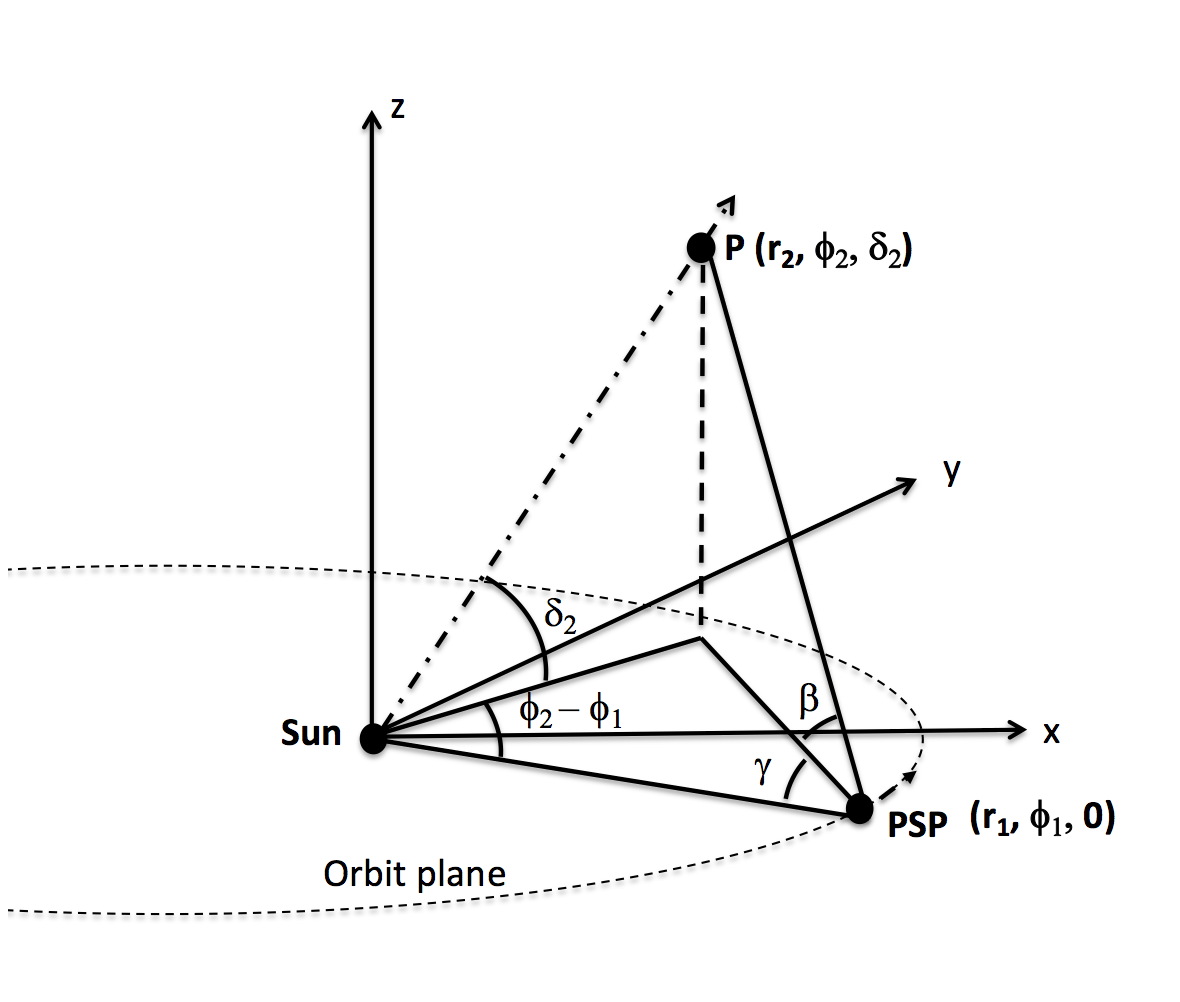
Figure 1.: Geometry relating the position of a feature P ($r2,\phi_{2},\delta_{2}$) in the HCI coordinate frame to the two angles $\gamma,\beta$ defining the unique line-of-sight from PSP to the feature P under the assumption that PSP’s orbit lies in the solar equatorial plane. (Adapted from Paper I.)fig:hci

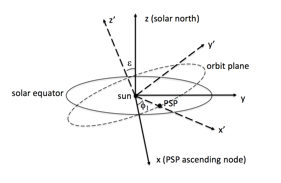
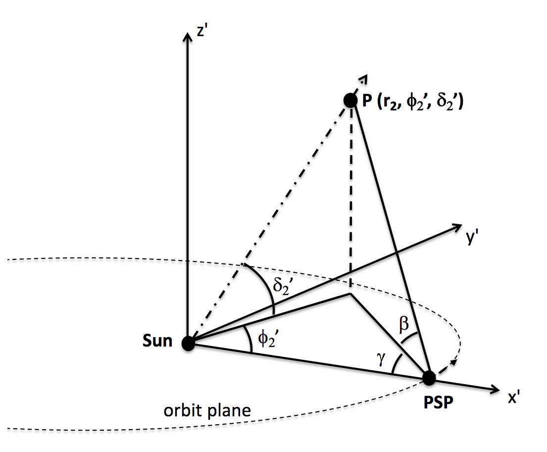
Figure 2.: Left: Geometry showing the relation of the HCI frame to the PSP orbital frame, where the inclination $\epsilon$ between the solar equatorial and PSP orbit planes exaggerated for clarity. Solid lines show the HCI coordinate frame ($xyz$) in which the $z$-axis is solar north and the $x$-axis points to the ascending node of PSP’s orbit. Dashed lines show the heliocentic frame ($x^{\prime}y^{\prime}z^{\prime}$) where the $x^{\prime}-y^{\prime}$ plane is PSP’s orbital plane and $x^{\prime}$ points to PSP. Right: Geometry showing the coordinates of feature P in the ($x^{\prime}y^{\prime}z^{\prime}$) frame.fig:tran1

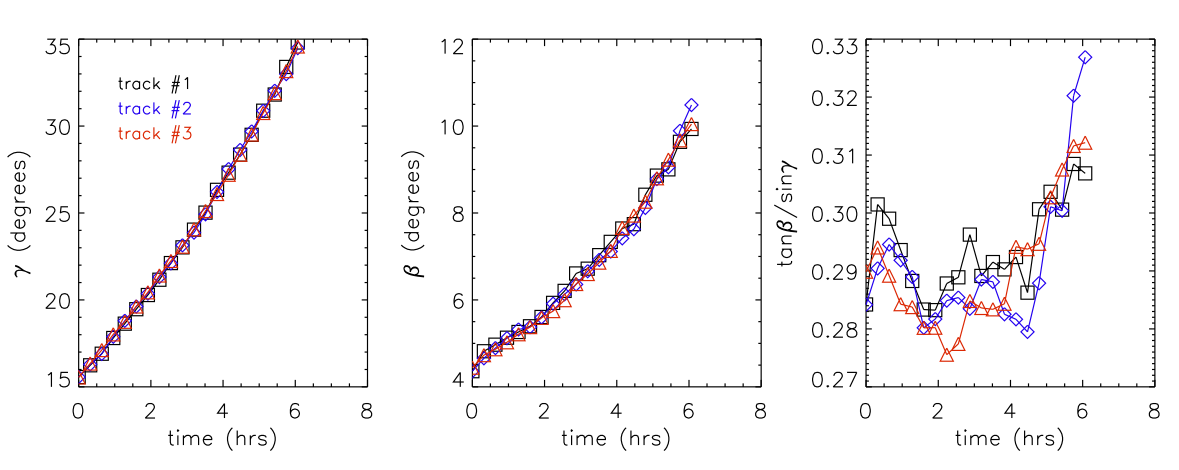
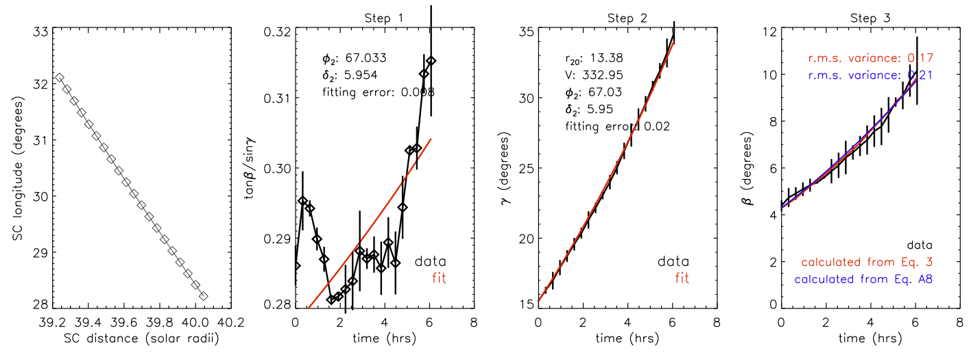
Figure 3.: Tracking and fitting results for the flux rope observed on 2019 April 2 (see Section 3.1 for details), which exhibits motion out of the orbit plane. The top row shows three independent trackings that return the $[\gamma(t_{i}),\beta(t_{i})]$ measurements. The bottom row shows the results of the two-step fit using the mean and uncertainties of the $[\gamma(t_{i}),\beta(t_{i})]$ measurements. The left panel shows the PSP’s longitude in the HCI frame and distance to the Sun during the observation; the second panel shows the first-step fit to Equation eq:3 to determine the two angles $\phi_{2}$ and $\delta_{2}$ of the tracked feature; the third panel shows the second-step fit to Equation eq:4 to determine $r_{20}$ and $V$ of the feature; and the last panel compares the $\beta(t_{i})$ calculated using Equation eq:3 (red) or Equation eq:a5 (blue) with observed values. Error bars (or uncertainties) in the plots are calculated using $[\gamma(t_{i}),\beta(t_{i})]$ measurements from the three independent different, multiplied by five for clarity. The quoted fitting error refers to the root-mean-square variance of the residuals of the fit.fig:ex1

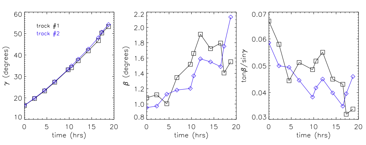
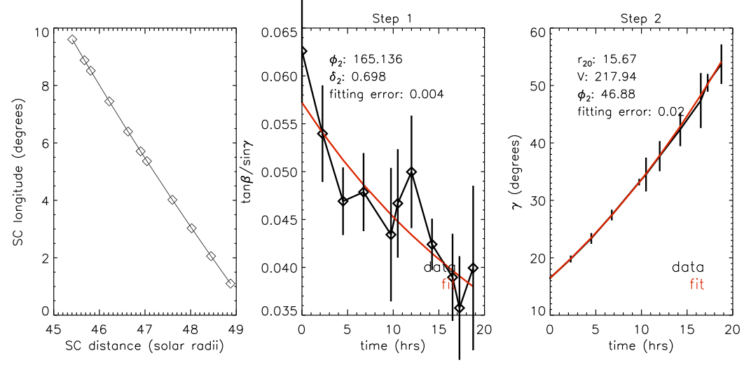
Figure 4.: Same as Figure fig:ex1; tracking (top) and fitting (bottom) results for the flux rope observed on 2018 November 1-2 (see Section 3.2 for details), which exhibits motion nearly in the orbit plane. For this case, the first-step fit (the second panel in the bottom row) returns a small value of $\delta_{2}$, thus the fitting results from the first-step are discarded, and $\phi_{2},r_{20}$, and $V$ are determined from a one-step fit to Eq. eq:4 with a fixed $\delta_{2}$ value (the third panel in the bottom row). $\delta_{2}$ is computed using the $\phi_{2},r_{0},V$ values from the one-step fit (see text in Section 2.2.2). For clarity, the error bars plotted in the last panel are multiplied by five. fig:ex2

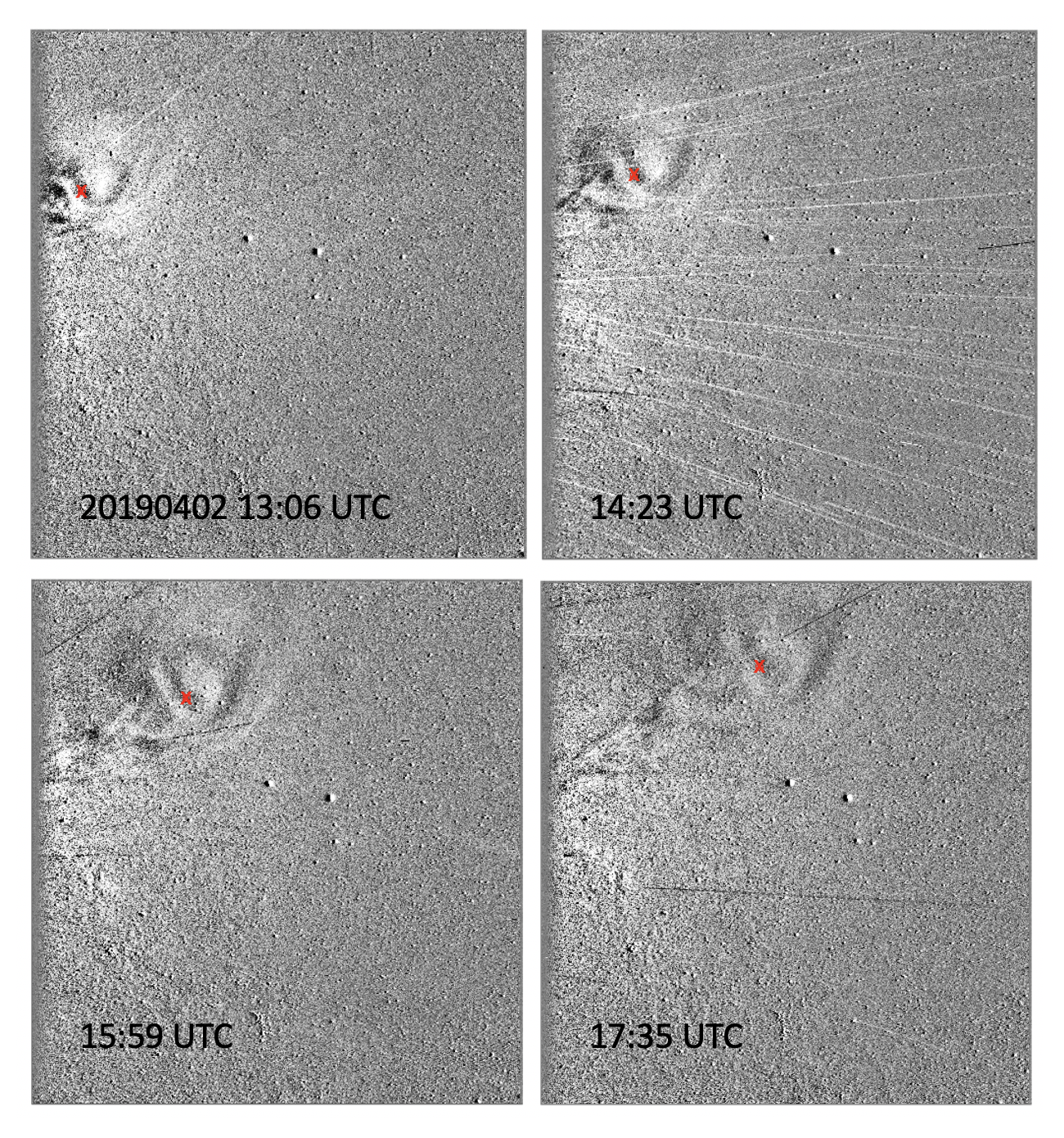
Figure 5.: WISPR-I running-difference images at four times for the CME of 2019 April 2. The tracked feature, the lower dark “eye” is marked with red X’s. The streaks seen especially in the image at 14:23 are caused by dust created by impacts on the spacecraft.fig:5

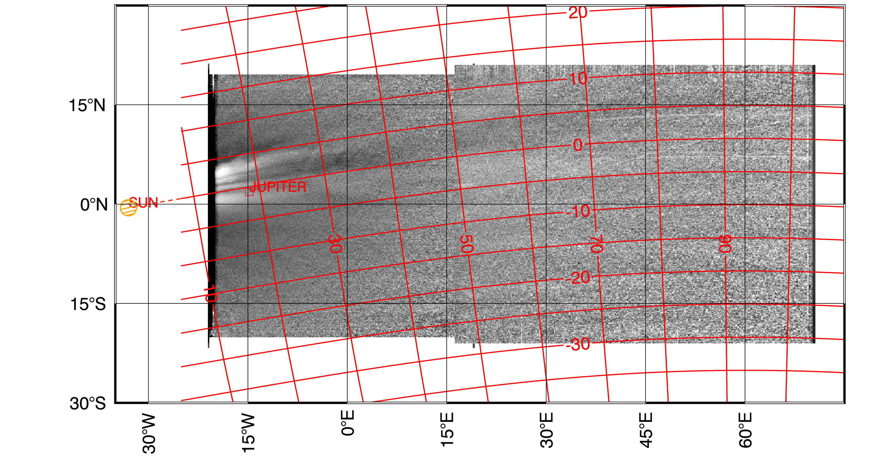
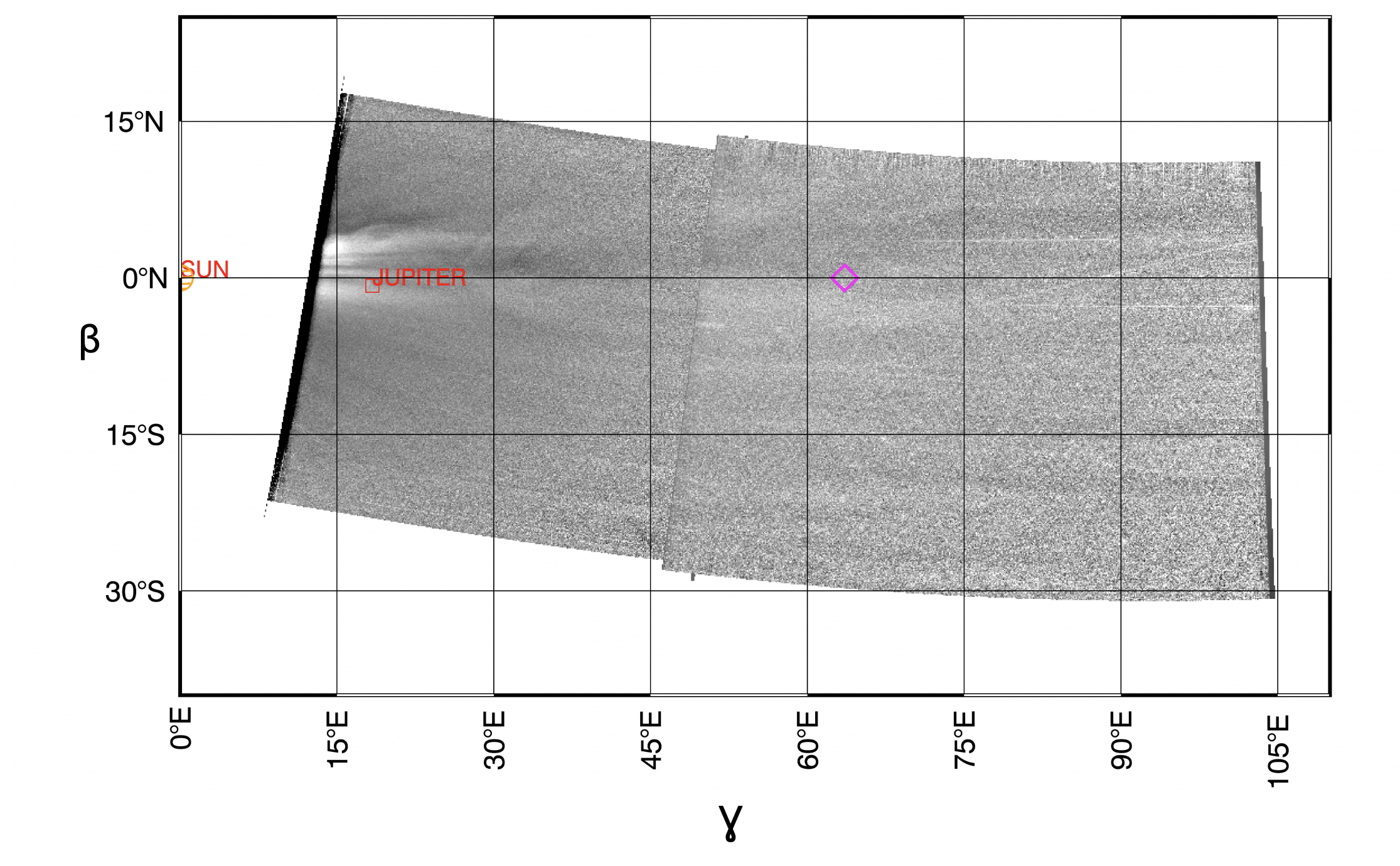
Figure 6.: Top: Combined WISPR-I and WISPR-O images of a CME in the inner telescope camera frame (black grid lines) in which the two angles, which define the lines-of-sight, are measured relative to the inner telescope centerline at (0,0). The Sun is shown 13^∘ further west than the inner edge of the FOV. The red grid is an overlay of the $\gamma-\beta$ grid lines of the PSP orbital frame where $\beta=0$ is PSP’s orbit plane, $\gamma$ is the angle in the plane, $\beta$ is the angle out of the plane, and the Sun is at ($\gamma,\beta)=(0,0)$. Bottom: The same images re-projected into the $\gamma-\beta$ PSP orbital frame (black grid lines). The magenta diamond marks the direction of the PSP velocity vector at this time (2018 November 1 at 22 UTC).

. fig:6

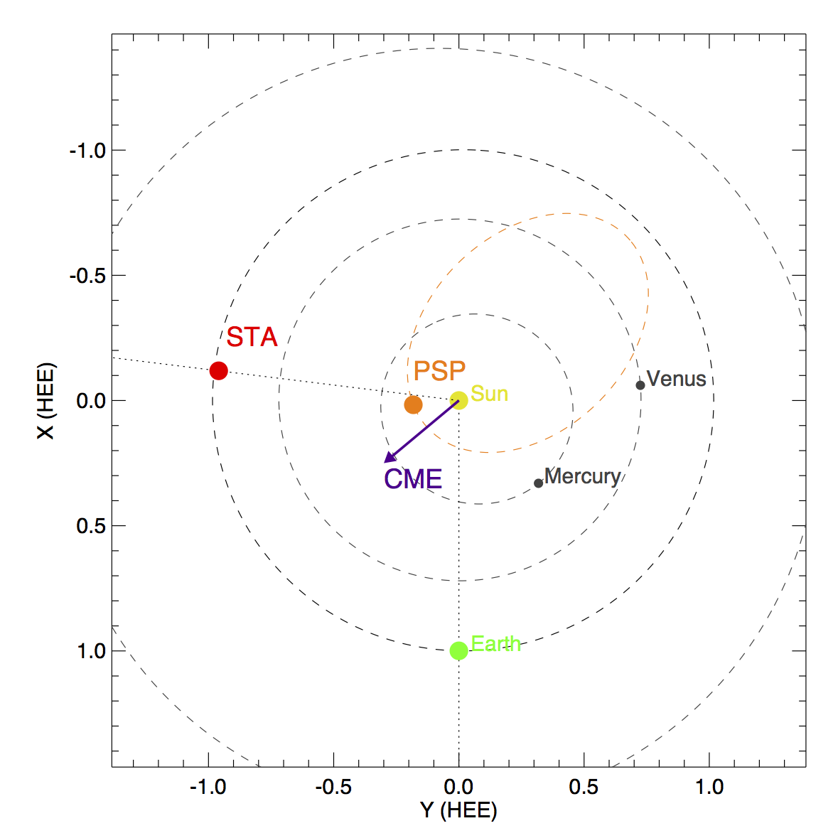
Figure 7.: Trajectory of 2019 April 2 flux rope in relation to PSP, STEREO-A and Earth, projected in the Heliocentric Earth Ecliptic (HEE) reference frame. The tracking/fitting solution gave the CME propagation direction to be HCI longitude $=67^{\circ}\pm 1^{\circ}$. Note that the purple arrow only indicates the direction of the CME, and is not meant to indicate the distance to the Sun. The HCI longitudes of the Earth and STA are 117^∘ and 19^∘, respectively. The orange dashed ellipse is PSP’s orbit. fig:7

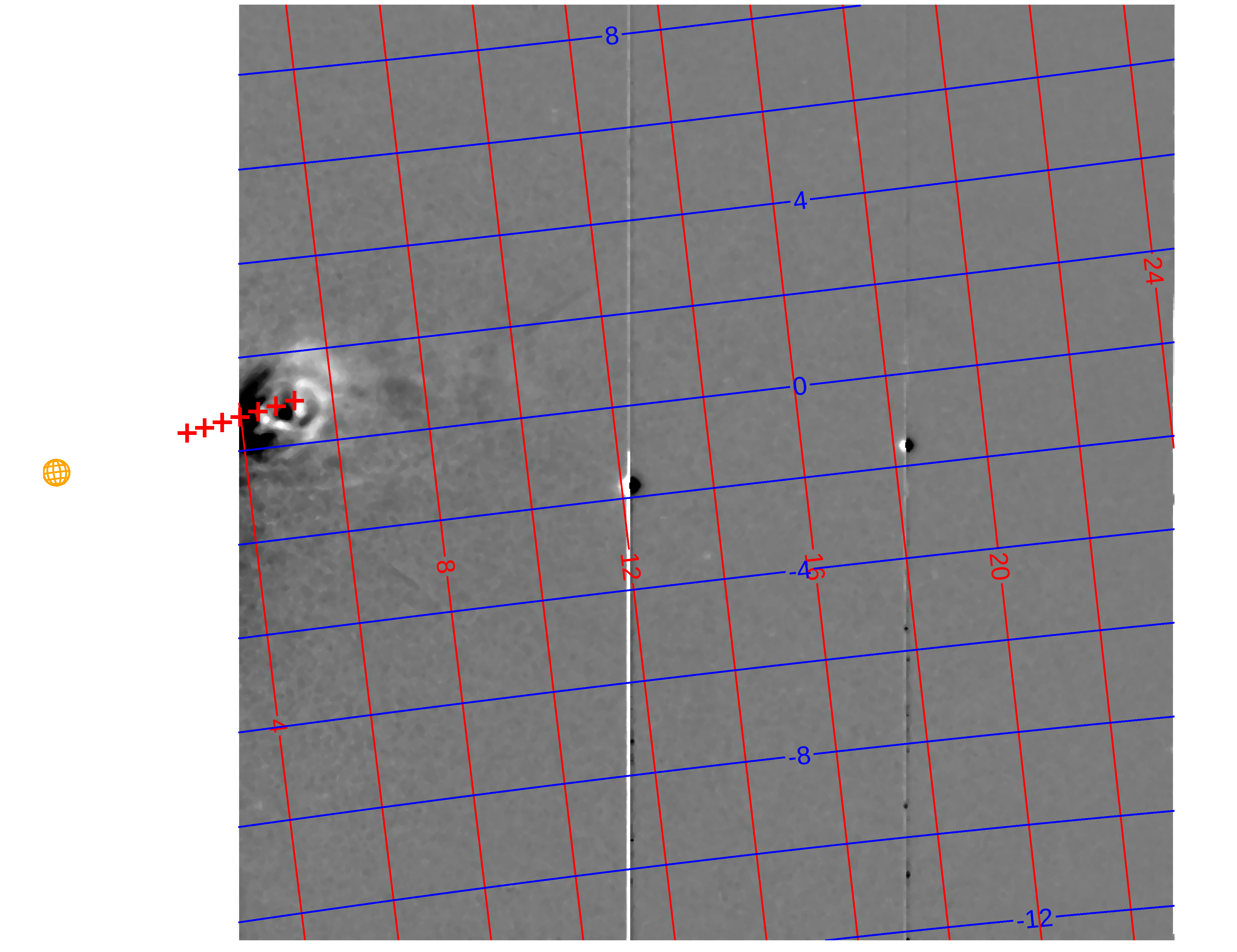
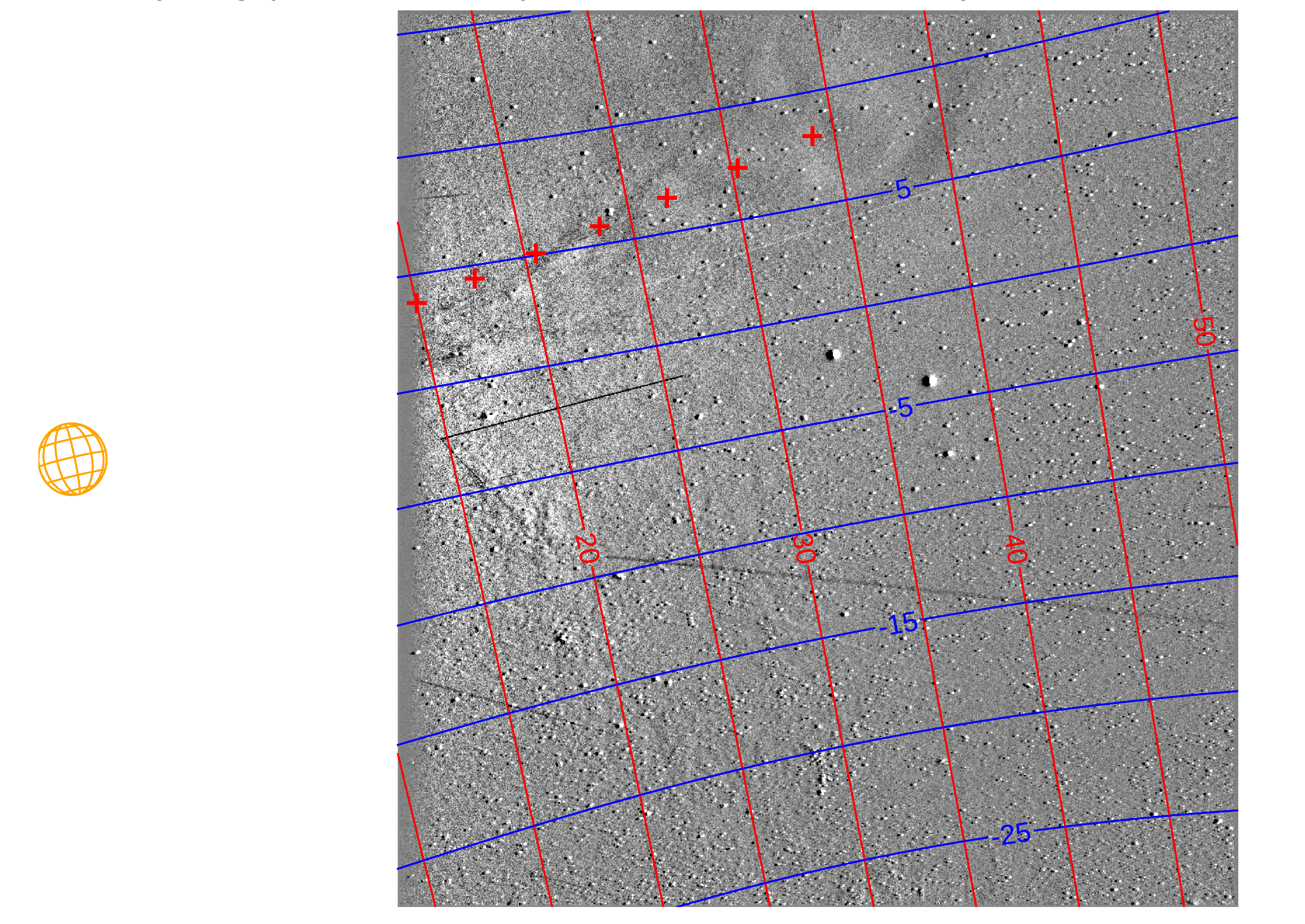
Figure 8.: Trajectory of the flux rope on 2019 April 2 predicted using the tracking/fitting technique projected to images from STEREO-A/HI-1 (top, 18:09 UTC), and WISPR-I (bottom, 18:13 UTC). The predicted trajectory (red +’s) is shown from 12:09 to 18:09 UTC in hourly increments. The location of the prediction for the last time (18:09 UTC) is in good agreement with the location of the tracked feature seen in the HI-1A image, as well as the WISPR image. In both images, the grid lines show helioprojective coordinates. In both images, the size and location of the Sun (yellow globe) are shown to scale.fig:8

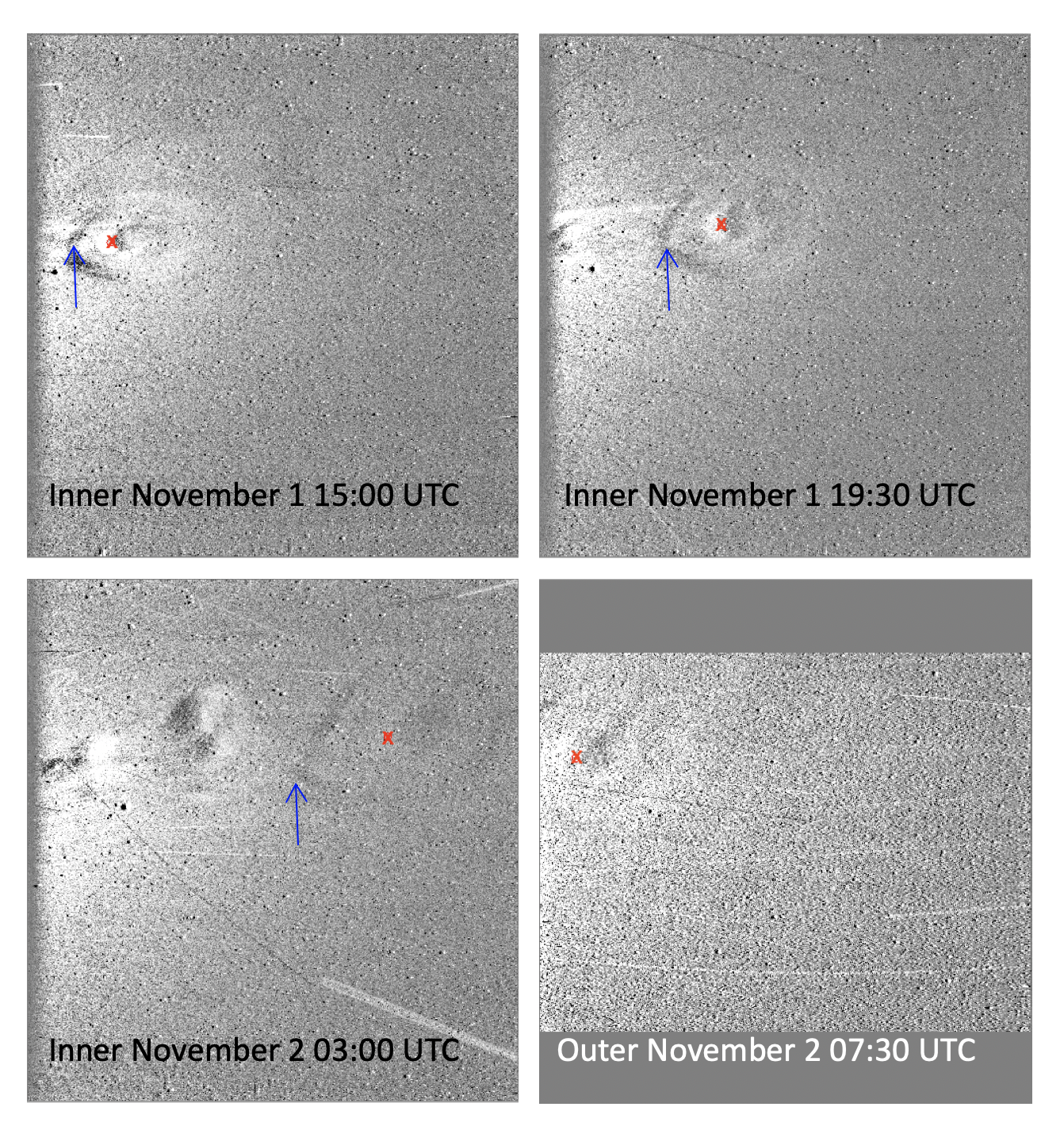
Figure 9.: WISPR running-difference images at four times for the CME of 2018 November 1-2; the first three are from WISPR-I and the last from WISPR-O. The pixel location of first tracked feature (the back edge of the dark cavity) is marked with red X’s. The blue arrow points to a second feature tracked, the tail end of the flux rope, to compare with tracking/fitting results of the first feature (see Section 4).fig:9

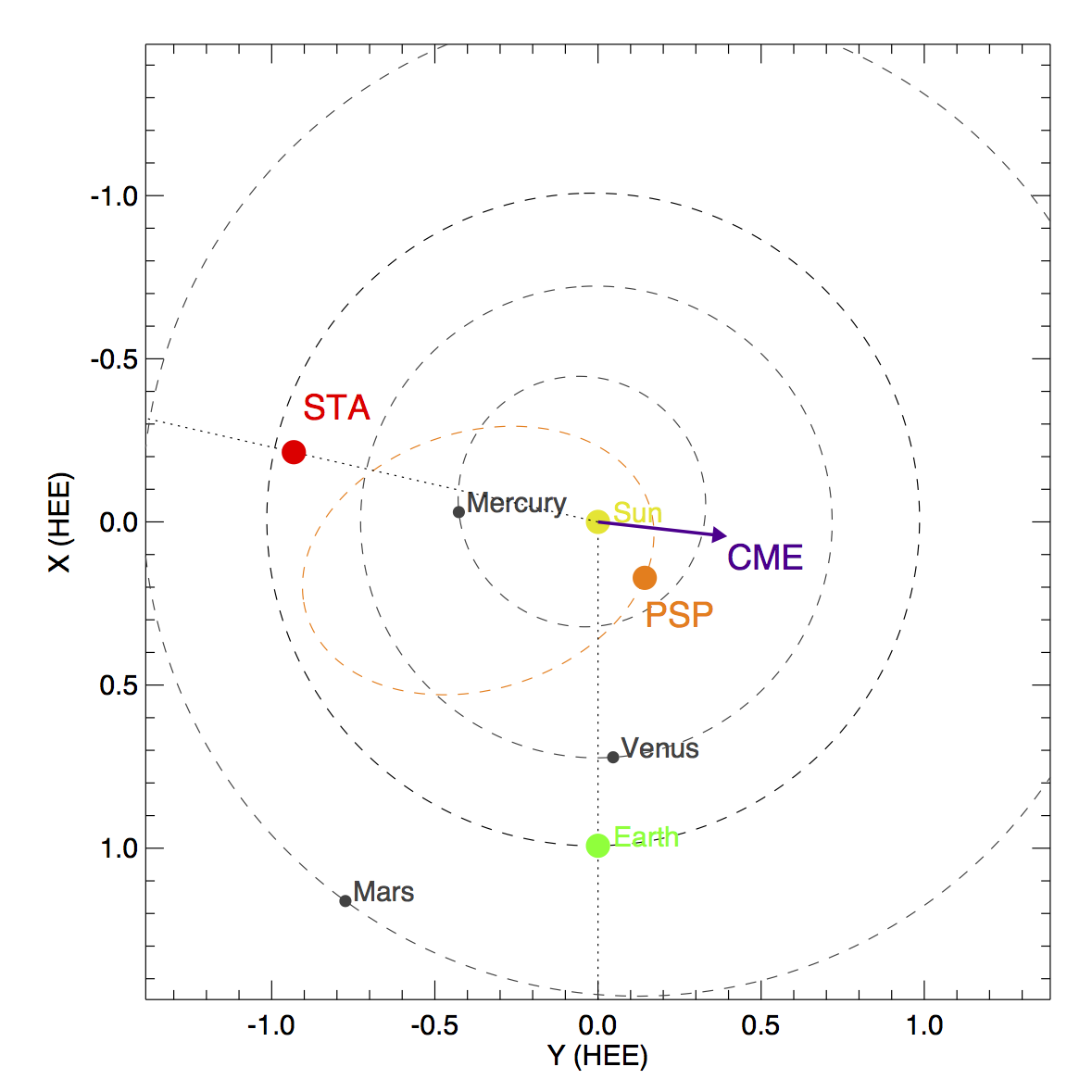
Figure 10.: Plot showing the direction of the flux rope, as determined by the tracking/fitting technique, with respect to PSP, STEREO-A, and Earth for 2018 November 1 at 17:15 UTC, projected in the Heliocentric Earth Ecliptic (HEE) reference frame. The CME propagation direction was found to be HCI longitude $=47^{\circ}\pm 2^{\circ}$. Note that the purple arrow only indicates the direction of the CME, and is not meant to indicate the distance to the Sun. The HCI longitudes of Earth and PSP are $-37^{\circ}$ and 3^∘, respectively. The orange dashed ellipse is PSP’s orbit.fig:10

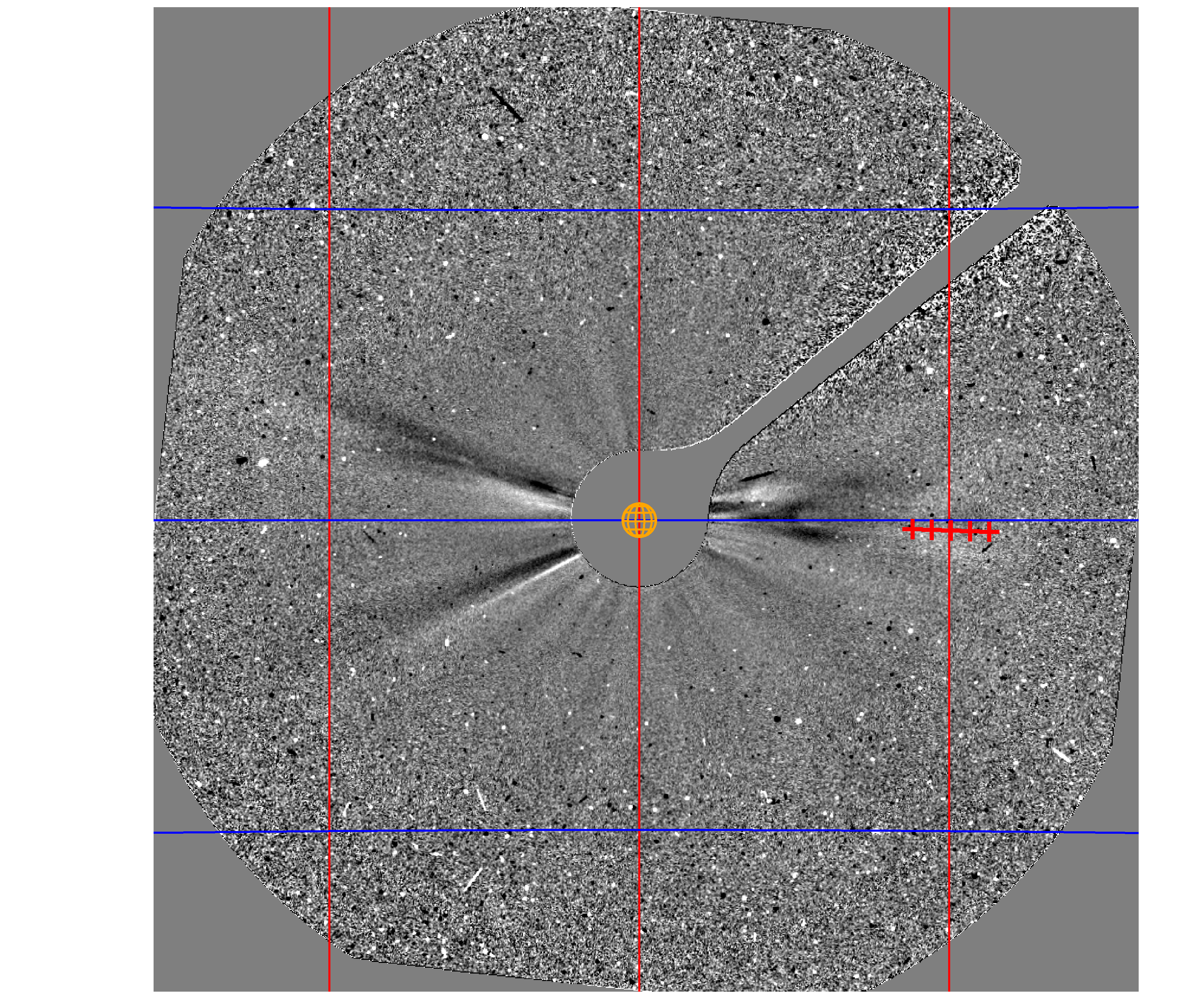
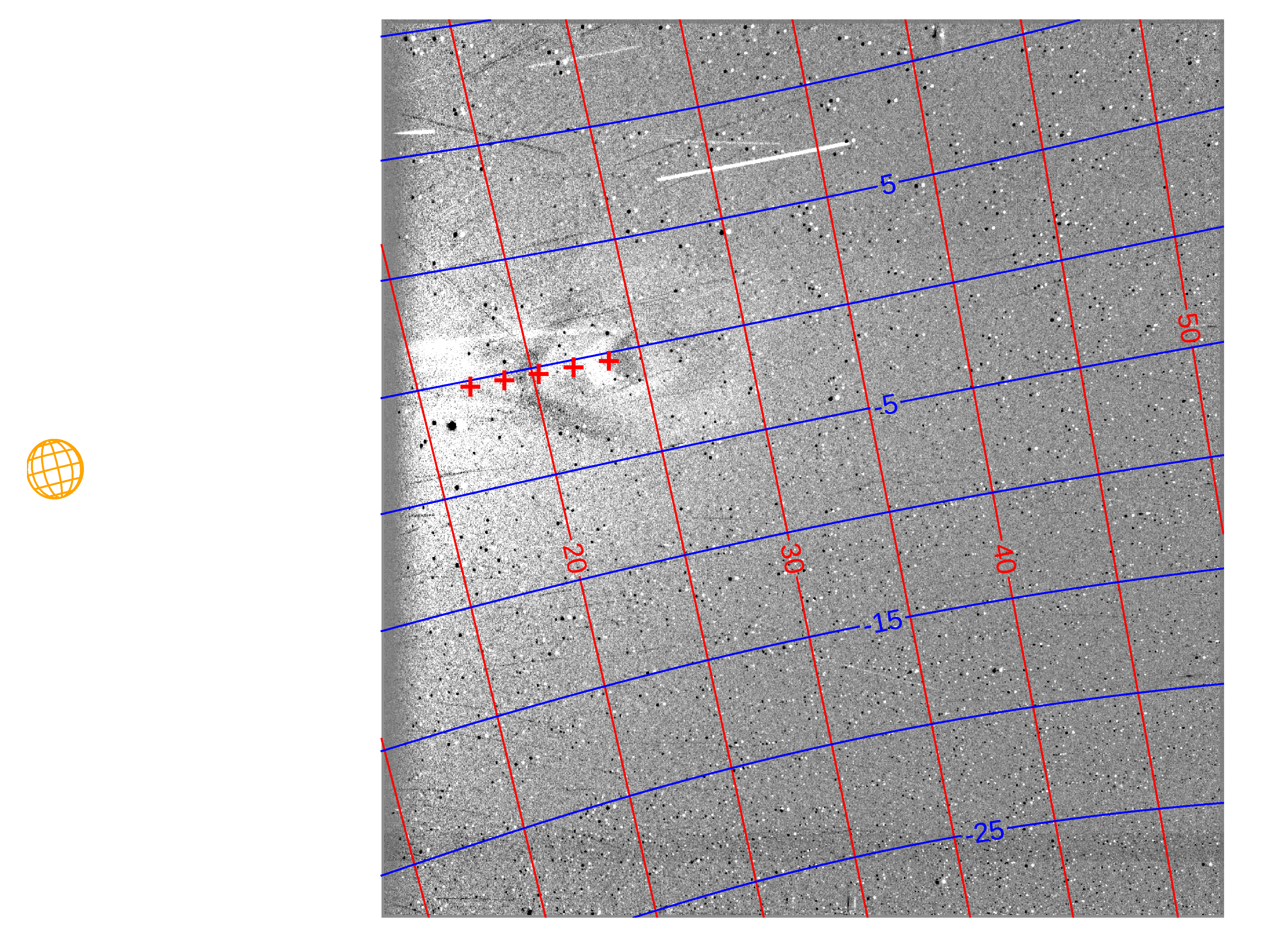
Figure 11.: Top: Predicted location of the back of the flux rope cavity for 2018 November 1 from 13:15 to 17:15 UTC in hourly increments projected onto a LASCO/C3 image at 17:16 UTC. The predicted distance of the feature from Sun for C3 is off by about 2 hrs or 2 R_⊙. Bottom: the same predicted trajectory points are plotted on a WISPR-I image at 17:15 UTC, used in tracking the flux rope. In both images, the grid lines show helioprojective coordinates.fig:11

References

- Conlon, Milan, and Davies (2014) Conlon, T.M., Milan, S.E., Davies, J.A.: 2014, Assessing the Effect of Spacecraft Motion on Single-Spacecraft Solar Wind Tracking Techniques. Sol. Phys. 289, 3935. DOI. ADS.
- Fox et al. (2016) Fox, N.J., Velli, M.C., Bale, S.D., Decker, R., Driesman, A., Howard, R.A., Kasper, J.C., Kinnison, J., Kusterer, M., Lario, D., Lockwood, M.K., McComas, D.J., Raouafi, N.E., Szabo, A.: 2016, The Solar Probe Plus Mission: Humanity’s First Visit to Our Star. Space Sci. Rev. 204, 7. DOI. ADS.
- Hess et al. (2020) Hess, P., Rouillard, A.P., Kouloumvakos, A., Liewer, P.C., Zhang, J., Dhakal, S., Stenborg, G., Colaninno, R.C., Howard, R.A.: 2020, WISPR Imaging of a Pristine CME. ApJS 246, 25. DOI. ADS.
- Howard et al. (2008) Howard, R.A., Moses, J.D., Vourlidas, A., Newmark, J.S., Socker, D.G., Plunkett, S.P., Korendyke, C.M., Cook, J.W., Hurley, A., Davila, J.M., Thompson, W.T., St Cyr, O.C., Mentzell, E., Mehalick, K., Lemen, J.R., Wuelser, J.P., Duncan, D.W., Tarbell, T.D., Wolfson, C.J., Moore, A., Harrison, R.A., Waltham, N.R., Lang, J., Davis, C.J., Eyles, C.J., Mapson-Menard, H., Simnett, G.M., Halain, J.P., Defise, J.M., Mazy, E., Rochus, P., Mercier, R., Ravet, M.F., Delmotte, F., Auchere, F., Delaboudiniere, J.P., Bothmer, V., Deutsch, W., Wang, D., Rich, N., Cooper, S., Stephens, V., Maahs, G., Baugh, R., McMullin, D., Carter, T.: 2008, Sun Earth Connection Coronal and Heliospheric Investigation (SECCHI). Space Sci. Rev. 136, 67. DOI. ADS.
- Howard et al. (2019) Howard, R.A., Vourlidas, A., Bothmer, V., Colaninno, R.C., DeForest, C.E., Gallagher, B., Hall, J.R., Hess, P., Higginson, A.K., Korendyke, C.M., Kouloumvakos, A., Lamy, P.L., Liewer, P.C., Linker, J., Linton, M., Penteado, P., Plunkett, S.P., Poirier, N., Raouafi, N.E., Rich, N., Rochus, P., Rouillard, A.P., Socker, D.G., Stenborg, G., Thernisien, A.F., Viall, N.M.: 2019, Near-Sun observations of an F-corona decrease and K-corona fine structure. Nature 576, 232. DOI. ADS.
- Liewer et al. (2011) Liewer, P.C., Hall, J.R., Howard, R.A., De Jong, E.M., Thompson, W.T., Thernisien, A.: 2011, Stereoscopic analysis of STEREO/SECCHI data for CME trajectory determination. Journal of Atmospheric and Solar-Terrestrial Physics 73, 1173. DOI. ADS.
- Liewer et al. (2019) Liewer, P., Vourlidas, A., Thernisien, A., Qiu, J., Penteado, P., Nisticò, G., Howard, R., Bothmer, V.: 2019, Simulating White Light Images of Coronal Structures for WISPR/ Parker Solar Probe: Effects of the Near-Sun Elliptical Orbit. Sol. Phys. 294, 93. DOI. ADS.
- Lugaz (2010) Lugaz, N.: 2010, Accuracy and Limitations of Fitting and Stereoscopic Methods to Determine the Direction of Coronal Mass Ejections from Heliospheric Imagers Observations. Sol. Phys. 267, 411. DOI. ADS.
- Nisticò et al. (2020) Nisticò, G., Bothmer, V., Vourlidas, A., Liewer, P.C., Thernisien, A.F., Stenborg, G., Howard, R.A.: 2020, Simulating White-Light Images of Coronal Structures for Parker Solar Probe/WISPR: Study of the Total Brightness Profiles. Sol. Phys. 295, 63. DOI. ADS.
- Patsourakos, Vourlidas, and Stenborg (2010) Patsourakos, S., Vourlidas, A., Stenborg, G.: 2010, The Genesis of an Impulsive Coronal Mass Ejection Observed at Ultra-high Cadence by AIA on SDO. ApJ 724, L188. DOI. ADS.
- Rouillard et al. (2008) Rouillard, A.P., Davies, J.A., Forsyth, R.J., Rees, A., Davis, C.J., Harrison, R.A., Lockwood, M., Bewsher, D., Crothers, S.R., Eyles, C.J., Hapgood, M., Perry, C.H.: 2008, First imaging of corotating interaction regions using the STEREO spacecraft. Geophys. Res. Lett. 35, L10110. DOI. ADS.
- Rouillard et al. (2009) Rouillard, A.P., Savani, N.P., Davies, J.A., Lavraud, B., Forsyth, R.J., Morley, S.K., Opitz, A., Sheeley, N.R., Burlaga, L.F., Sauvaud, J.-A., Simunac, K.D.C., Luhmann, J.G., Galvin, A.B., Crothers, S.R., Davis, C.J., Harrison, R.A., Lockwood, M., Eyles, C.J., Bewsher, D., Brown, D.S.: 2009, A Multispacecraft Analysis of a Small-Scale Transient Entrained by Solar Wind Streams. Sol. Phys. 256, 307. DOI. ADS.
- Savani et al. (2012) Savani, N.P., Davies, J.A., Davis, C.J., Shiota, D., Rouillard, A.P., Owens, M.J., Kusano, K., Bothmer, V., Bamford, S.P., Lintott, C.J., Smith, A.: 2012, Observational Tracking of the 2D Structure of Coronal Mass Ejections Between the Sun and 1 AU. Sol. Phys. 279, 517. DOI. ADS.
- Sheeley et al. (2008) Sheeley, J. N. R., Herbst, A.D., Palatchi, C.A., Wang, Y.-M., Howard, R.A., Moses, J.D., Vourlidas, A., Newmark, J.S., Socker, D.G., Plunkett, S.P., Korendyke, C.M., Burlaga, L.F., Davila, J.M., Thompson, W.T., St. Cyr, O.C., Harrison, R.A., Davis, C.J., Eyles, C.J., Halain, J.P., Wang, D., Rich, N.B., Battams, K., Esfandiari, E., Stenborg, G.: 2008, Heliospheric Images of the Solar Wind at Earth. ApJ 675, 853. DOI. ADS.
- Sheeley et al. (1999) Sheeley, N.R., Walters, J.H., Wang, Y.-M., Howard, R.A.: 1999, Continuous tracking of coronal outflows: Two kinds of coronal mass ejections. J. Geophys. Res. 104, 24739. DOI. ADS.
- Thompson (2006) Thompson, W.T.: 2006, Coordinate systems for solar image data. A&A 449, 791. DOI. ADS.
- Vourlidas et al. (2016) Vourlidas, A., Howard, R.A., Plunkett, S.P., Korendyke, C.M., Thernisien, A.F.R., Wang, D., Rich, N., Carter, M.T., Chua, D.H., Socker, D.G., Linton, M.G., Morrill, J.S., Lynch, S., Thurn, A., Van Duyne, P., Hagood, R., Clifford, G., Grey, P.J., Velli, M., Liewer, P.C., Hall, J.R., DeJong, E.M., Mikic, Z., Rochus, P., Mazy, E., Bothmer, V., Rodmann, J.: 2016, The Wide-Field Imager for Solar Probe Plus (WISPR). Space Sci. Rev. 204, 83. DOI. ADS.
- Zhu et al. (2020) Zhu, C., Qiu, J., Liewer, P., Vourlidas, A., Spiegel, M., Hu, Q.: 2020, How Does Magnetic Reconnection Drive the Early-stage Evolution of Coronal Mass Ejections? ApJ 893, 141. DOI. ADS.
. \ilabelfig:6