Efficient Certification of Spatial Robustness

Abstract

Recent work has exposed the vulnerability of computer vision models to vector field attacks. Due to the widespread usage of such models in safety-critical applications, it is crucial to quantify their robustness against such spatial transformations. However, existing work only provides empirical robustness quantification against vector field deformations via adversarial attacks, which lack provable guarantees. In this work, we propose novel convex relaxations, enabling us, for the first time, to provide a certificate of robustness against vector field transformations. Our relaxations are model-agnostic and can be leveraged by a wide range of neural network verifiers. Experiments on various network architectures and different datasets demonstrate the effectiveness and scalability of our method.

1 Introduction

It was recently shown that neural networks are susceptible not only to standard noise-based adversarial perturbations (Szegedy et al. 2014; Goodfellow, Shlens, and Szegedy 2015; Carlini and Wagner 2017; Madry et al. 2018) but also to spatially transformed images that are visually indistinguishable from the original (Kanbak, Moosavi-Dezfooli, and Frossard 2018; Alaifari, Alberti, and Gauksson 2019; Xiao et al. 2018; Engstrom et al. 2019). Such spatial attacks can be modeled by smooth vector fields that describe the displacement of every pixel. Common geometric transformations, e.g., rotation and translation, are particular instances of these smooth vector fields, which indicates that they capture a wide range of naturally occurring image transformations.

Since the vulnerability of neural networks to spatially transformed adversarial examples can pose a security threat to computer vision systems relying on such models, it is critical to quantify their robustness against spatial transformations. A common approach to estimate neural network robustness is to measure the success rate of strong attacks (Carlini and Wagner 2017; Madry et al. 2018). However, many networks that are indeed robust against these attacks were later broken using even more sophisticated attacks (Athalye and Carlini 2018; Athalye, Carlini, and Wagner 2018; Engstrom, Ilyas, and Athalye 2018; Tramèr et al. 2020). The key issue is that such attacks do not provide provable robustness guarantees.

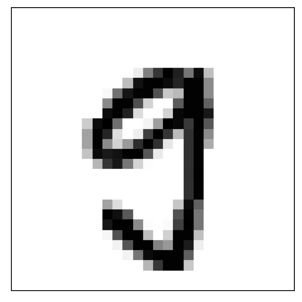
(a) Original

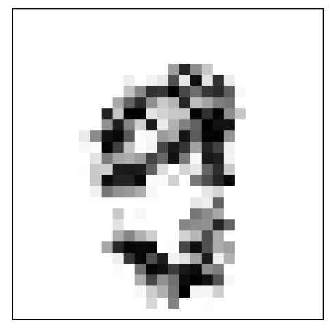
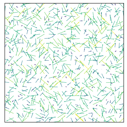
(b) $\delta=1$, $\gamma=\infty$

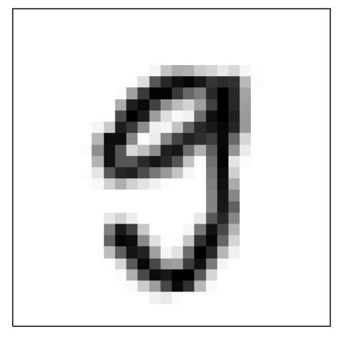
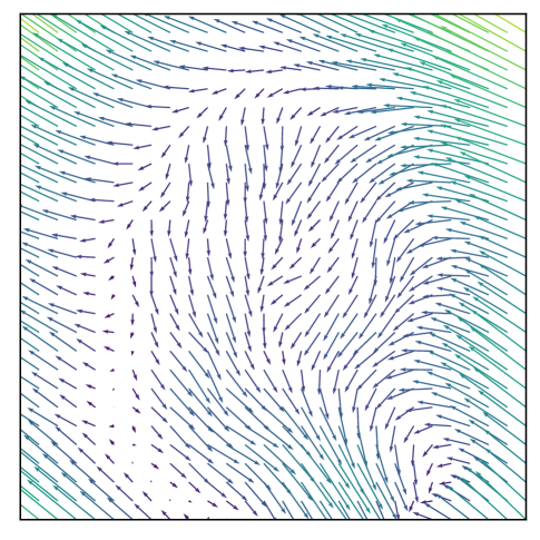
(c) $\delta=3$, $\gamma=0.25$

Figure 1: Image instances and corresponding deforming vector fields ($\gamma$ and $\delta$ explained below): (a) original, (b) adversarially deformed (label 5) by non-smooth vector field, and (c) adversarially deformed (label 3) by smooth vector field.

To address this issue, our goal is to provide a provable certificate that a neural network is robust against all possible deforming vector fields within an attack budget for a given dataset of images. While various certification methods exist, they are limited to noise-based perturbations (Katz et al. 2017; Gehr et al. 2018; Wong and Kolter 2018; Singh et al. 2018; Zhang et al. 2018) or compositions of common geometric transformations (e.g., rotations and translations) (Pei et al. 2017; Singh et al. 2019b; Balunovic et al. 2019; Mohapatra et al. 2020) and thus cannot be applied to our setting.

A common approach in robustness certification is to compute, for a given image, pixel bounds containing all possible perturbed images within some attack budget, and then propagate these bounds through the network to obtain bounds on the output neurons. Then, if all images within the output bounds classify to the correct label, the network is provably robust against all attacks limited to the same attack budget. In our work, we intuitively parametrize the attack budget by the magnitude of pixel displacement, denoted by $\delta$, and the smoothness of the vector field, denoted by $\gamma$. This allows us to efficiently compute the tightest-possible pixel interval bounds on vector field deformations limited to a given displacement magnitude $\delta$ by using a mathematical analysis of the transformation. However, even small but non-smooth vector fields (i.e., small $\delta$ but large $\gamma$) can generate large pixel differences, resulting in recognizably perturbed images (Figure 1(b)) and leading to large pixel bounds, which limit certification performance. Thus, a key challenge is to define smoothness constraints that can be efficiently incorporated with neural network verifiers to enable certification of smooth vector fields with large displacement magnitude (Figure 1(c)).

Hence, we tighten our convex relaxation for smooth vector fields by introducing smoothness constraints that can be efficiently incorporated into state-of-the-art verifiers (Tjeng, Xiao, and Tedrake 2019; Singh et al. 2019a, c). To that end, we leverage the idea of computing linear constraints on the pixel values in terms of the transformation parameters (Balunovic et al. 2019; Mohapatra et al. 2020). We show that our mathematical analysis of the transformation induces an optimization problem for computing the linear constraints, which can be efficiently solved by linear programming. Finally, we show that the idea by Balunovic et al. (2019); Mohapatra et al. (2020) alone is insufficient for the setting of smooth vector fields, and only the combination with our smoothness constraints yields superior certification performance. We implement our method in an open-source system and show that our convex relaxations can be leveraged to, for the first time, certify neural network robustness against vector field attacks.

Key contributions

We make the following contributions:

• A novel method to compute the tight interval bounds for norm-constrained vector field attacks, enabling the first certification of neural networks against vector field attacks.

• A tightening of our relaxation for smooth vector fields and integration with state-of-the-art robustness certifiers.

• An open-source implementation together with extensive experimental evaluation on the MNIST and CIFAR-10 datasets, with convolutional and large residual networks. We make our code publicly available as part of the ERAN framework for neural network verification (available at https://github.com/eth-sri/eran).

2 Related Work

Here we discuss the most relevant related work on spatial robustness and certification of neural networks.

Empirical spatial robustness

In addition to previously known adversarial examples based on $\ell_{p}$-norm perturbations, it has recently been demonstrated that adversarial examples can also be constructed via geometric transformations (Kanbak, Moosavi-Dezfooli, and Frossard 2018), rotations and translations (Engstrom et al. 2019), Wasserstein distance (Wong, Schmidt, and Kolter 2019; Levine and Feizi 2020; Hu et al. 2020), and vector field deformations (Alaifari, Alberti, and Gauksson 2019; Xiao et al. 2018). Here, we use a threat model based on vector field deformations for which both prior works have proposed attacks: Alaifari, Alberti, and Gauksson (2019) perform first-order approximations to find minimum-norm adversarial vector fields, and Xiao et al. (2018) relax vector field smoothness constraints with a continuous loss to find perceptually realistic adversarial examples.

Robustness certification

There is a long line of work on certifying the robustness of neural networks to noise-based perturbations. These approaches employ SMT solvers (Katz et al. 2017), mixed-integer linear programming (Tjeng, Xiao, and Tedrake 2019; Singh et al. 2019c), semidefinite programming (Raghunathan, Steinhardt, and Liang 2018), and linear relaxations (Gehr et al. 2018; Wong and Kolter 2018; Singh et al. 2018; Zhang et al. 2018; Wang et al. 2018; Weng et al. 2018; Singh et al. 2019b; Salman et al. 2019b; Lin et al. 2019). Another line of work also considers certification via randomized smoothing (Lécuyer et al. 2019; Cohen, Rosenfeld, and Kolter 2019; Salman et al. 2019a), which, however, only provides probabilistic robustness guarantees for smoothed models whose predictions cannot be evaluated exactly, only approximated to arbitrarily high confidence.

Certified spatial robustness

Prior work introduces certification methods for special cases of spatial transformations: a finite number of transformations (Pei et al. 2017), rotations (Singh et al. 2019b), and compositions of common geometric transformations (Balunovic et al. 2019; Mohapatra et al. 2020). Some randomized smoothing approaches exist, but they only handle single parameter transformations (Li et al. 2020) or transformations without compositions (Fischer, Baader, and Vechev 2020). In a different setting, Wu and Kwiatkowska (2020) compute the maximum safe radius on optical flow video perturbations but only for a finite set of neighboring grid points. Overall, previous approaches are limited because they only certify transformations in specific templates that can be characterized as special cases of smooth vector field deformations. Certifying these vector field deformations is precisely the goal of our work.

While rotations are special cases of smooth deformations, even small rotations can cause not only large pixel displacements (i.e., large $\delta$) far from the center of rotation but also large smoothness constraints (i.e., large $\gamma$) due to the singularity at the center of rotation. Since such large $\gamma$ and $\delta$ values are currently out of reach for our method, we advise using specialized certification methods (Balunovic et al. 2019; Mohapatra et al. 2020) when considering threat models consisting only of rotations. However, we could combine our approach with these specialized certification methods, e.g., by instantiating DeepG (Balunovic et al. 2019) with our interval bounds, which would correspond to first deforming an image by a vector field and then rotating the deformed image.

3 Background

Here we introduce our notation, define the similarity metric for spatially transformed images, and provide the necessary background for neural network certification.

Vector field deformations

We represent an image as a function $I\colon P\subseteq{\mathbb{R}}^{2}\rightarrow{\mathbb{R}}^{C}$, where $C$ is the number of color channels, and $P=\{1,2,\ldots,W\}^{2}$ corresponds to the set of pixel coordinates of the image with dimension $W\times W$.

Vector field transformations are parameterized by a vector field $\tau\colon P\rightarrow{\mathbb{R}}^{2}$ assigning a displacement vector $\tau(i,j)$ to every pixel $(i,j)$. Thus, we obtain the deformed pixel coordinates via $(\mathbb{I}+\tau)\colon P\rightarrow\mathbb{R}^{2}$ with $(\mathbb{I}+\tau)(i,j)=(i,j)+\tau(i,j)$, where $\mathbb{I}$ is the identity operator. Since these deformed coordinates may not lie on the integer grid, we use bilinear interpolation $\mathcal{I}_{I}:{\mathbb{R}}^{2}\rightarrow{\mathbb{R}}^{C}$ induced by the image $I$ and evaluated at $(i,j)+\tau(i,j)$ to get the deformed pixel values:

$$\mathcal{I}_{I}\left(i,j\right) :=\begin{cases}\mathcal{I}_{I}^{mn}\left(i,j\right)&\text{if}\left(i,j\right)\in A_{mn}\end{cases},$$

$$\mathcal{I}^{mn}_{I}\left(i,j\right) :=\sum_{\begin{subarray}{c}p\in\left\{m,m+1\right\}\\ q\in\left\{n,n+1\right\}\end{subarray}}I(p,q)\left(1-\lvert p-i\rvert\right)\left(1-\lvert q-j\rvert\right),$$ (1)

where $A_{mn}:=\left[m,m+1\right]\times\left[n,n+1\right]$ is an interpolation region. Hence, we define the deformed image as $\mathcal{I}_{I}\circ\left(\mathbb{I}+\tau\right)$. Like Alaifari, Alberti, and Gauksson (2019), we only study vector fields that do not move pixels outside the image.

Estimating perceptual similarity

For noise-based adversarial attacks, an adversarial image $I_{adv}$ is typically considered perceptually similar to the original image $I$ if the $\ell_{p}$-norm of the perturbation $\left\|I-I_{adv}\right\|_{p}$ is small (Szegedy et al. 2014; Goodfellow, Shlens, and Szegedy 2015; Carlini and Wagner 2017; Madry et al. 2018). However, prior work (Alaifari, Alberti, and Gauksson 2019; Xiao et al. 2018) has demonstrated that this is not necessarily a good measure for spatially transformed images. For example, translating an image by a small amount will typically produce an image that looks very similar to the original but results in a large perturbation with respect to the $\ell_{p}$-norm. For this reason, the similarity of spatially transformed images is typically estimated with a norm on the deforming vector field and not on the pixel value perturbation. Here, we consider the $T_{p}$-norm (Alaifari, Alberti, and Gauksson 2019), defined as

$$\left\|\tau\right\|_{T_{p}}:=\max_{(i,j)\in P}\left\|\tau\left(i,j\right)\right\|_{p}.$$

We consider $p\in\{1,2,\infty\}$ and note that the case $p=2$ corresponds to the norm used by Alaifari, Alberti, and Gauksson (2019). Intuitively, a vector field with $T_{2}$-norm at most $1$ will displace any pixel by at most one grid length on the image grid. In general, for a vector field $\tau$ with $\left\|\tau\right\|_{T_{p}}\leq\delta$, the set of reachable coordinates from a single pixel $\left(i,j\right)\in P$ is

$$B_{\delta}^{p}\left(i,j\right):=\left\{x\in\mathbb{R}^{2}\mid\left\|\left(i,j\right)-x\right\|_{p}\leq\delta\right\}.$$

However, there may be vector fields with small $T_{p}$-norm that produce unrealistic images. For example, moving every pixel independently by at most one grid length can already result in very pixelated images that can be easily recognized as unnatural when comparing with the original (Figure 1(b)). To address this, Xiao et al. (2018) introduce a flow loss that penalizes the vector field’s lack of smoothness. Following this approach, we say that vector field $\tau$ has flow $\gamma$ if it satisfies, for each pixel $(i,j)$, the flow-constraints

$$||\tau(i,j)-\tau(i^{\prime},j^{\prime})||_{\infty}\leq\gamma,\forall\left(i^{\prime},j^{\prime}\right)\in\mathcal{N}(i,j),$$ (2)

where $\mathcal{N}(i,j)\subseteq P$ represents the set of neighboring pixels in the 4 cardinal directions of pixel $(i,j)$. For instance, translation is parametrized by a vector field that has flow $0$ (each pixel has the same displacement vector). These constraints enforce smoothness of the vector field $\tau$, which in turn ensures that transformed images look realistic and better preserve image semantics – even for large values of $\delta$ (Figure 1(c)). We provide a more thorough visual investigation of the norms and constraints considered in Appendix D.

Figure 2: Convex relaxation of a sample neural network with inputs $x_{0}$ and $x_{1}$, and vector field components $v_{x}$, $v_{y}$, $w_{x}$, and $w_{y}$.

Robustness certification

Robustness of neural networks is typically certified by (i) computing a convex shape around the input we want to certify (an over-approximation) and (ii) propagating this shape through all operations in the network to obtain a final output shape. Robustness is then proven if all concrete outputs inside the output shape classify to the correct class. For smaller networks, an input shape can be propagated exactly using mixed-integer linear programming (Tjeng, Xiao, and Tedrake 2019). To scale to larger networks, standard approaches over-approximate the shape using various convex relaxations: intervals (Gowal et al. 2019), zonotopes (Gehr et al. 2018; Singh et al. 2018; Weng et al. 2018), and restricted polyhedra (Zhang et al. 2018; Singh et al. 2019b), just to name a few. In this work, we build on the convex relaxation DeepPoly, an instance of restricted polyhedra, introduced by Singh et al. (2019b), as it provides a good trade-off between scalability to larger networks and precision. For every pixel, DeepPoly receives a lower and upper bound on the pixel value, i.e., an input shape in the form of a box. This shape is then propagated by maintaining one lower and upper linear constraint for each neuron. Here, we first show how to construct a tight box around all spatially transformed images. However, since this box does not capture the relationship between neighboring pixels induced by flow-constraints, it contains spurious images that cannot be produced by smooth vector fields. To address this, we tighten the convex relaxation for smooth vector fields by incorporating flow-constraints.

Problem statement

Our goal is to prove local robustness against vector field attacks constrained by maximal pixel displacement, i.e., all vector fields with $T$-norm smaller than $\delta$. That is, for every image from the test set, we try to compute a certificate that guarantees that no vector field with a displacement magnitude smaller than $\delta$ can change the predicted label. Furthermore, since smooth deformations are more realistic, we also consider the case where the vector fields additionally need to satisfy our flow-constraints, i.e., that neighboring deformation vectors can differ by at most $\gamma$ in $\ell_{\infty}$-norm.

4 Overview

We now provide an end-to-end example of how to compute our convex relaxation of vector field deformations and use it to certify the robustness of the toy network in Figure 2. This network propagates inputs $x_{0}$ and $x_{1}$ according to the weights annotated on the edges. Neurons $x_{2}$, $x_{3}$ and $x_{4}$, $x_{5}$ denote the pre- and post-activation values, and $x_{6}$, $x_{7}$ are the network logits. We augment this network by vector field components $v_{x}$, $v_{y}$, $w_{x}$, and $w_{y}$, to introduce the flow-constraints.

The concrete inputs to the neural network are the pixels marked with blue ($x_{0}$) and green ($x_{1}$), shown in Figure 3(a). The image is perturbed by a vector field of $T_{\infty}$-norm $\delta=0.5$ and flow $\gamma=0.25$. Thus the blue and green pixels are allowed to move in the respective rectangles shown in Figure 3(a). However, to satisfy the flow-constraints, their deformation vectors can differ by at most $\gamma=0.25$ in each coordinate.

Our objective is to certify that the neural network classifies the input to the correct label regardless of its deformed pixel positions. A simple forward pass of the pixel values $x_{0}=0$ and $x_{1}=0.5$ yields logit values $x_{6}=0$ and $x_{7}=0.625$. Assuming that the image is correctly classified, we thus need to prove that the value of neuron $x_{7}$ is greater than the value of neuron $x_{6}$ for all admissible smooth vector field transformations. To that end, we will first compute interval bounds for the pixels without using the relationship between vector field components $v_{x}$, $v_{y}$, $w_{x}$, and $w_{y}$, and then, in a second step, we tighten the relaxation for smooth vector fields by introducing linear constraints on $x_{0}$ and $x_{1}$ in terms of $v_{x}$, $v_{y}$, $w_{x}$, and $w_{y}$ to exploit the flow-constraint relationship. Propagation of our convex relaxation through the network closely follows Singh et al. (2019b), and we provide a full formalization of our methods in Section 5.

Calculating interval bounds

The first part of our convex relaxation is computing upper and lower interval bounds for the values that the blue and green pixel can attain on their $\ell_{\infty}$-neighborhood of radius $\delta=0.5$. For both pixels, the minimum and maximum are attained on the left and right border of the $\ell_{\infty}$-ball, respectively. Using bilinear interpolation from Equation 1, we thus obtain the interval bounds $[l_{0},u_{0}]=[0,0.25]$ for $x_{0}$ and $[l_{1},u_{1}]=[0.25,0.75]$ for $x_{1}$.

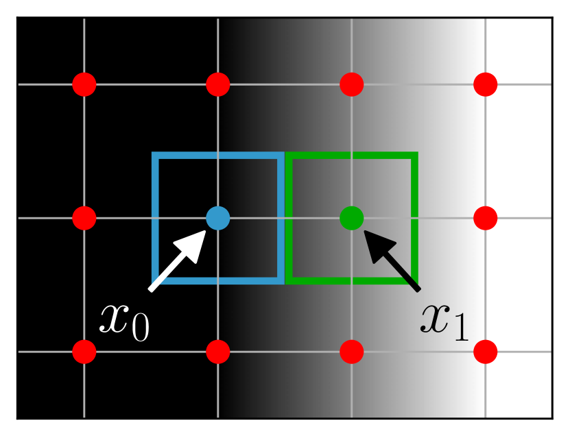
(a) Sample image

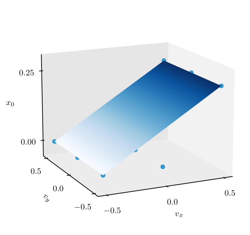
(b) Upper-bounding plane for $x_{0}$

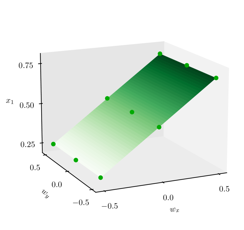
(c) Lower-bounding plane for $x_{1}$

Figure 3: Bilinear interpolation for a sample image with dots indicating pixel positions and squares denoting the set of reachable coordinates $B_{0.5}^{\infty}$ for pixels $x_{0}$ and $x_{1}$. Figures 3(b) and 3(c) display the interval bound candidates, i.e., the potential extrema of bilinear interpolation (see Section 5), as dots and the linear bounding planes used to enforce flow-constraints. Note that the candidates are computed separately for every intersection of an interpolation region with the set of reachable coordinates $B_{0.5}^{\infty}$.

Interval bound propagation

The intervals $[l_{0},u_{0}]$ and $[l_{1},u_{1}]$ can be utilized directly for verification using standard interval propagation to estimate the output of the network (Gehr et al. 2018; Gowal et al. 2019; Mirman, Gehr, and Vechev 2018). While this method is fast, it is also imprecise. The interval bounds for $x_{2}$ and $x_{4}$ are

$$[l_{2},u_{2}] =2\cdot[l_{0},u_{0}]-[l_{1},u_{1}]+0.25$$

$$=[2l_{0}-u_{1}+0.25,2u_{0}-l_{1}+0.25]=[-0.5,0.5],$$

$$[l_{4},u_{4}] =[\max(l_{2},0),\max(u_{2},0)]=[0,0.5].$$

All lower and upper interval bounds are given in Figure 2. The output for $x_{6}$ is thus between $l_{6}=-1$ and $u_{6}=0$, while the one for $x_{7}$ is between $l_{7}=-0.375$ and $u_{7}=0.875$. As this is insufficient to prove $x_{7}>x_{6}$, certification fails.

Backsubstitution

To gain precision, one can keep track of the relationship between the neurons by storing linear constraints (Zhang et al. 2018; Singh et al. 2019b). In addition to $[l_{2},u_{2}]$, we store upper- and lower-bounding linear constraints

$$2x_{0}-x_{1}+0.25\leq x_{2}\leq 2x_{0}-x_{1}+0.25.$$

Similarly, for $x_{4}$, we store, in addition to $[l_{4},u_{4}]$,

$$0\leq x_{4}\leq 0.5x_{2}+0.25,$$

where we use the rules given in Singh et al. (2019b) to calculate the upper and lower linear constraints. All linear constraints are shown in Figure 2, next to the corresponding neurons. Certification succeeds, if we can show that $x_{7}-x_{6}>0$. Using the linear constraints, we thus obtain

$$x_{7}-x_{6} \geq(-x_{4}+x_{5})-(-2x_{4})=x_{4}+x_{5}$$

$$\geq x_{3}\geq x_{1}-x_{0}+0.125\geq 0.125.$$

This proves that $x_{7}-x_{6}>0$, implying that the network classifies to the correct class under all considered deformations.

Spatial constraints

Although the above method can certify robustness, certification fails for a more challenging network where the bias of $x_{3}$ is equal to $-0.125$ instead of $0.125$. With the previous approach, we can only prove $x_{7}-x_{6}\geq x_{1}-x_{0}-0.125\geq-0.125$, which is insufficient for certification. However, we can leverage our vector field smoothness condition (Equation 2), namely that the deformation vectors of $x_{0}$ and $x_{1}$ can differ by at most $\gamma=0.25$ in the $\ell_{\infty}$-norm. Unfortunately, these constraints cannot be directly applied since they are defined on the vector field components and not on the pixel values. To amend this, we build on the idea from Balunovic et al. (2019); Mohapatra et al. (2020) and add upper- and lower-bounding linear constraints on the pixel values $x_{0}$ and $x_{1}$. That is, we compute upper and lower planes in terms of vector field components $v_{x}$ and $v_{y}$ for $x_{0}$ and $w_{x}$ and $w_{y}$ for $x_{1}$, as shown in Figures 3(b) and 3(c). The plane equations are shown in Figure 2, and details on the computation are provided in Section 5. By substituting these plane equations into our expression and considering that all vector field components $v_{x}$, $v_{y}$, $w_{x}$, and $w_{y}$ are bounded from above and below by $[-\delta,\delta]=[-0.5,0.5]$, we thus obtain

$$x_{7}-x_{6} \geq x_{1}-x_{0}-0.125$$

$$\geq(0.5+0.5w_{x})-(0.125+0.25v_{x})-0.125$$

$$=0.25+0.5w_{x}-0.25v_{x}\geq-0.125,$$

showing that a simple instantiation of the idea by Balunovic et al. (2019); Mohapatra et al. (2020) is insufficient for certification in our setting. Only with our flow-constraints $-\gamma\leq v_{x}-w_{x}\leq\gamma$ with $\gamma=0.25$ can we finally certify:

$$x_{7}-x_{6} \geq x_{1}-x_{0}-0.125$$

$$\geq 0.25+0.5w_{x}-0.25v_{x}$$

$$=0.25+0.25w_{x}+0.25(w_{x}-v_{x})\geq 0.0625.$$

In practice, the resulting expression may have more than two pixels, and we use a linear program (described in Section 5) to perform the substitution of flow-constraints.

5 Convex Relaxation

Here, we introduce a novel convex relaxation tailored to vector field deformations. First, we compute the tightest interval bounds for each pixel in the transformed image. As intervals do not capture dependencies between variables, we then propose a method for introducing linear constraints on the pixel values in terms of vector field components and show how to use flow-constraints to further tighten our convex relaxation.

5.1 Computing Tight Interval Constraints

Consider an image $I$ and a maximum pixel displacement $\delta$. Our goal is to compute, for pixel $(i,j)$, interval bounds $l_{i,j}$ and $u_{i,j}$ such that $l_{i,j}\leq\mathcal{I}_{I}\circ(\mathbb{I}+\tau)(i,j)\leq u_{i,j}$, for any vector field $\tau$ of $T_{p}$-norm at most $\delta$. We now show how to compute tight interval pixel bounds $[l_{i,j},u_{i,j}]$.

Within a given interpolation region $A_{mn}$, the pixel $(i,j)$ can move to positions in $B_{\delta}^{p}(i,j)\cap A_{mn}$. Thus, for every pixel, we construct a set of candidates containing the possible maxima and minima of that pixel in $B_{\delta}^{p}(i,j)\cap A_{mn}$. However, this could potentially yield an infinite set of candidate points, and we thus make the key observation that the minimum and maximum pixel values of $\mathcal{I}^{mn}_{I}$ in $B_{\delta}^{p}(i,j)\cap A_{mn}$ are always obtained at the boundary (see Lemma 5.1 below, with proof provided in Appendix A). Hence, for any reachable interpolation region $A_{mn}$, it suffices to consider the boundary of $B_{\delta}^{p}(i,j)\cap A_{mn}$ to derive the candidate points analytically. Finally, we set the lower and upper bound of the pixel value to the minimum and maximum of the candidate set, respectively.

Lemma 5.1.

The minimum and maximum pixel values of $\mathcal{I}^{mn}_{I}$ in $B_{\delta}^{p}(i,j)\cap A_{mn}$ are always obtained at the boundary.

We note that it is essential to calculate the candidates analytically to guarantee the soundness of our interval bounds. Furthermore, for a single-channel image, our interval bounds are exact, i.e., for every deformed image within our pixel bounds there exists a corresponding vector field $\tau$ with $||\tau||_{p}\leq\delta$. For the derivation of candidates, we make use of the following auxiliary lemma (with proof in Appendix A):

Lemma 5.2.

The bilinear interpolation $\mathcal{I}^{mn}_{I}(v,w)$ on the region $A_{mn}$ can be rewritten as

$$\mathcal{I}^{mn}_{I}(v,w)=A+Bv+Cw+Dvw.$$ (3)

Candidates for $T_{\infty}$

The boundary of $B_{\delta}^{\infty}(i,j)\cap A_{mn}$ consists of line segments parallel to the coordinate axes. This means that for all pixels $(v,w)$ on such a line segment either $v$ or $w$ is constant. Thus, according to Equation 3, if $v$ is fixed, then $\mathcal{I}^{mn}_{I}$ is linear in $w$ and vice-versa. Hence, we only need to consider the line segment endpoints to obtain the candidate set of all possible extremal values in $B_{\delta}^{\infty}(i,j)\cap A_{mn}$.

Candidates for $T_{1}$

The boundary of $B_{\delta}^{1}(i,j)\cap A_{mn}$ consists of line segments parallel to the coordinate axes or lines defined by $w=\pm v+a$. In the first case, we add the pixel values of the line segment endpoints to the set of candidates. In the second case, the bilinear interpolation $\mathcal{I}^{mn}_{I}$ restricted to $w=\pm v+a$ is a polynomial of degree $2$ given by

$$\mathcal{I}^{mn}_{I}(v,\pm v+a) =A+Bv+C(\pm v+a)+Dv(\pm v+a)$$

$$=(A+Ca)+(B\pm C)v\pm Dv^{2}.$$

Thus, the extremum can be attained on the interior of that line, unlike the $T_{\infty}$-case. Hence, we add both the endpoint values and the polynomial’s extremum to the candidate set if the corresponding extremal point lies on the line segment.

Candidates for $T_{2}$

The boundary of $B_{\delta}^{2}(i,j)\cap A_{mn}$ consists of line segments parallel to the coordinate axes or an arc with circle center $(i,j)$. We handle the line segments by adding the pixel values at the endpoints to the candidate set. However, the interpolation can also have minima and maxima on the interior of the arc. To find those, we extend the interpolation $\mathcal{I}^{mn}_{I}$ from $A_{mn}$ to $\mathbb{R}^{2}$ and use Lagrange multipliers to find the extrema on the circle $v^{2}+w^{2}=\delta^{2}$ (assuming $i=j=0$ for notational convenience). The Lagrangian is

$$\Lambda(v,w,\lambda):=\mathcal{I}^{mn}_{I}\left(v,w\right)-\lambda(v^{2}+w^{2}-\delta^{2}),$$

which yields

$$\nabla_{v,w,\lambda}\Lambda(v,w,\lambda)=\begin{pmatrix}B+Dw-2\lambda v\\ C+Dv-2\lambda w\\ \delta^{2}-v^{2}-w^{2}\\ \end{pmatrix}\stackrel{{\scriptstyle!}}{{=}}0.$$

Solving the first two equations for $\lambda$, we obtain

$$\lambda=\frac{B+Dw}{2v}\quad\text{and}\quad\lambda=\frac{C+Dv}{2w},$$

assuming $v\neq 0\neq w$ (else $\delta=0$). Eliminating $\lambda$, we have

$$w(B+Dw)-v(C+Dv)=0.$$

We solve this quadratic equation and substitute the solutions

$$w=\frac{-B\pm\sqrt{B^{2}+4Dv(C+Dv)}}{2D}.$$

into $\delta^{2}-v^{2}-w^{2}=0$ to obtain

$$\delta^{2}=v^{2}+\left(\frac{-B\pm\sqrt{B^{2}+4Dv(C+Dv)}}{2D}\right)^{2}.$$

Setting $E:=\frac{-B}{2D}$, $F:=\frac{B^{2}}{4D^{2}}$, and $G:=\frac{C}{D}$ we have

$$\delta^{2} =v^{2}+\left(E\pm\sqrt{F+Gv+v^{2}}\right)^{2}$$

$$=v^{2}+E^{2}\pm 2E\sqrt{F+Gv+v^{2}}+F+Gv+v^{2}$$

$$=2v^{2}+Gv\pm 2E\sqrt{F+Gv+v^{2}}+H,$$

for $H:=(E^{2}+F)$. Solving for $v$ requires squaring both sides to resolve the square root, yielding

$$\left(\delta^{2}-H-Gv-2v^{2}\right)^{2} =\left(\pm 2E\sqrt{F+Gv+v^{2}}\right)^{2}$$

$$=4E^{2}(F+Gv+v^{2}).$$

Thus, we are interested in finding the roots of

$$J+Kv+Lv^{2}+Mv^{3}+Nv^{4}$$ (4)

with

$$J :=\left(\delta^{2}-H\right)^{2}-4FE^{2},$$

$$K :=-2G\left(\left(\delta^{2}-H\right)+2E^{2}\right),$$

$$L :=G^{2}-4\left(\left(\delta^{2}-H\right)+E^{2}\right)$$

$$M :=4G$$

$$N :=4,$$

which is a polynomial of degree $4$. The roots of a polynomial of degree $4$ are known in closed form (Shmakov 2011), and we use Durand-Kerner’s root finding method (Kerner 1966) to compute them analytically. We recall that computing the roots approximately, e.g., via gradient descent or Newton’s method, does not guarantee the soundness of our interval bounds. If the coordinates obtained from the roots of Equation 4 lie within $A_{mn}$, we add the corresponding pixel values to the set of candidates. Finally, we add the pixel values of the endpoints of the arc to the set of candidates.

5.2 Computing Spatial Constraints

While our interval bounds are tight, they can contain spurious images, which cannot be produced by smooth vector fields of flow $\gamma$. To address this, we build upon the idea of Balunovic et al. (2019); Mohapatra et al. (2020) and introduce linear constraints on the pixel values in terms of the vector field, which can then be paired with flow-constraints to yield a tighter convex relaxation. We demonstrate how our method can be applied to tighten the DeepPoly relaxation (Singh et al. 2019b) and robustness certification via mixed-integer linear programming (MILP) (Tjeng, Xiao, and Tedrake 2019).

		MNIST						CIFAR-10
		ConvSmall PGD		ConvSmall DiffAI		ConvBig DiffAI		ConvSmall DiffAI		ConvMed DiffAI
$\delta$	$\gamma$	DeepPoly	MILP	DeepPoly	MILP	DeepPoly	MILP	DeepPoly	MILP	DeepPoly	MILP
0.3	$\infty$	51	97	90	91	90	91	40	47	51	56
	0.1	78	98	90	92	90	94	45	56	53	60
	0.01	91	99	91	95	91	95	50	70	57	70
	0.001	92	98	92	95	91	95	53	71	58	73
0.4	$\infty$	6	89	74	76	78	84	31	38	36	42
	0.1	40	91	75	84	78	90	32	46	37	51
	0.01	75	98	77	92	78	90	35	67	43	57
	0.001	77	99	77	92	78	92	37	69	43	58
0.5	$\infty$	0	76	40	50	36	62	20	32	29	34
	0.1	7	85	44	69	37	79	23	47	30	42
	0.01	32	88	44	91	37	89	27	53	31	47
	0.001	35	89	44	92	37	90	27	53	33	48

Table 1: $T_{\infty}$-norm certification rates (%) for vector fields $\tau$ with displacement magnitude $\|\tau\|_{T_{\infty}}=\delta$ and flow $\gamma$.

Upper- and lower-bounding planes

We seek to compute sound linear constraints on the spatially transformed pixel value in terms of the deforming vector field $\tau$. Since every pixel is displaced independently by its corresponding vector, the linear constraints induce bounding planes of the form

$$\lambda_{0}+\lambda\cdot\tau(i,j)\leq\mathcal{I}_{I}((i,j)+\tau(i,j))\leq\upsilon_{0}+\upsilon\cdot\tau(i,j),$$

where $\lambda^{T}=(\lambda_{1},\lambda_{2})$ and $\upsilon^{T}=(\upsilon_{1},\upsilon_{2})$. To compute a sound lower-bounding plane, we apply our method from Section 5.1 to compute the set of candidate coordinates $\mathcal{C}$ of potential minima and maxima in $B_{\delta}^{\infty}(i,j)$ and then solve

$$\operatorname*{arg\,min}_{\lambda_{0},\lambda_{1},\lambda_{2}}\sum_{(p,q)\in\mathcal{C}}\mathcal{I}_{I}(p,q)-(\lambda_{0}+\lambda_{1}(p-i)+\lambda_{2}(q-j))$$

$$\mathcal{I}_{I}(p,q)\geq(\lambda_{0}+\lambda_{1}(p-i)+\lambda_{2}(q-j)),\quad\forall(p,q)\in\mathcal{C}.$$

Since both the objective and the constraints are linear, we can compute this plane in polynomial time using linear programming. The upper-bounding plane is obtained analogously.

Given these linear bounding planes, one could be tempted to simply instantiate the framework from Balunovic et al. (2019); Mohapatra et al. (2020). Unfortunately, their approach only works in the setting where multiple pixels are transformed by the same spatial parameters (e.g., rotation angle). However, we make the key observation that these linear constraints can be leveraged to enforce the flow-constraints, thus tightening our convex relaxation. We now describe how this can be achieved for the DeepPoly relaxation and MILP.

Tightening DeepPoly relaxation

To compute precise bounds, DeepPoly performs backsubstitution for each neuron in the network (recall the example in Section 4). That is, every backsubstitution step computes a linear expression $e=a_{1}x_{1}+\ldots+a_{n}x_{n}$ in terms of the input pixels. A naive way to obtain the upper and lower bounds of $e$ is to substitute the interval bounds for each pixel $x_{i}$, which is equivalent to

$$\min a_{1}x_{1}+\ldots+a_{n}x_{n}$$

$$l_{i}\leq x_{i}\leq u_{i}.$$

However, this can be imprecise as intervals do not capture flow-constraints. Thus, we extend the above linear program with variables $v_{x}^{(i)}$ and $v_{y}^{(i)}$ denoting the vector field components of every pixel $x_{i}$, thus allowing us to add the constraints

$$\lambda_{0}^{(i)}+(v_{x},v_{y})^{(i)}\lambda^{(i)}\leq x_{i}\leq\upsilon_{0}^{(i)}+(v_{x},v_{y})^{(i)}\upsilon^{(i)},$$ (5)

$$-\gamma\leq v_{x}^{(i)}-v_{x}^{(j)}\leq\gamma,\text{ and }-\gamma\leq v_{y}^{(i)}-v_{y}^{(j)}\leq\gamma,$$ (6)

where $\lambda^{T}=(\lambda_{1}^{(i)},\lambda_{2}^{(i)})$ and $\upsilon^{T}=(\upsilon_{1}^{(i)},\upsilon_{2}^{(i)})$. Here, Equation 5 corresponds to the upper- and lower-bounding planes of pixel $x_{i}$, and Equation 6 enforces the flow-constraints for neighboring pixels $i$ and $j$. Minimization of this linear program then directly yields the tightest lower bound on the expression and can be performed in polynomial time. The upper-bounding plane can be obtained analogously.

Tightening MILP certification

To encode a neural network as MILP, we employ the method from Tjeng, Xiao, and Tedrake (2019), which is exact for models with ReLU activations. Our approach of leveraging linear planes on pixel values to enforce flow-constraints can then be directly applied to the resulting MILP by adding the same variables and linear constraints (Equations 5 and 6) as in the DeepPoly case.

6 Experiments

We now investigate the precision and scalability of our certification method by evaluating it on a rich combination of datasets and network architectures. We make all our networks and code publicly available as part of the ERAN framework for neural network verification (available at https://github.com/eth-sri/eran) to ensure reproducibility.

Experiment setup

We select a random subset of 100 images from the MNIST (LeCun, Cortes, and Burges 2010) and CIFAR-10 (Krizhevsky 2009) test datasets on which we run all experiments. We consider adversarially trained variants of the ConvSmall, ConvMed, and ConvBig architectures proposed by Mirman, Gehr, and Vechev (2018), using PGD (Madry et al. 2018) and DiffAI (Mirman, Gehr, and Vechev 2018) for adversarial training. For CIFAR-10, we also consider a ResNet (He et al. 2016), with 4 residual blocks of 16, 16, 32, and 64 filters each, trained with the provable defense from Wong et al. (2018). We present the model accuracies and training hyperparameters in Appendix B. While we only consider networks with ReLU activations for our experiments, our relaxations seamlessly integrate with different verifiers, including DeepPoly, k-ReLU, and MILP, which allows us to certify all networks employing the activation functions supported by these frameworks. For example, DeepPoly handles ReLU, sigmoid, tanh, quadratic, and logarithmic activations, while MILP can only exactly encode piecewise linear activation functions such as ReLU or LeakyReLU. We use a desktop PC with a single GeForce RTX 2080 Ti GPU and a 16-core Intel(R) Core(TM) i9-9900K CPU @ 3.60GHz, and we report all certification running times in Appendix C.

Robustness certification

We demonstrate the precision of our convex relaxations via robustness certification against vector field transformations. To that end, we run DeepPoly and MILP with our interval and spatial constraints and compute the percentage of certified MNIST and CIFAR-10 images for different networks and values of $\delta$ and $\gamma$. Note that $\gamma=\infty$ corresponds to Section 5.1, and $\gamma<\infty$ corresponds to Section 5.2. We limit MILP to 5 minutes and display the results in Table 1 (showing only $T_{\infty}$-norm results for brevity). We observe that our interval bounds successfully enable certification of vector field attacks and that our tightened convex relaxation for smooth vector fields offers (at times substantial) improvements across all datasets, verifiers, and networks. For example, for ConvSmall PGD on MNIST, DeepPoly certification increases from $6\%$ ($\gamma=\infty$) to $77\%$ ($\gamma=0.001$) for $\delta=0.4$. Similarly, for ConvSmall DiffAI on CIFAR-10, MILP certification increases from $38\%$ ($\gamma=\infty$) to $69\%$ ($\gamma=0.001$) for $\delta=0.4$. In fact, our convex relaxation can also be applied with the k-ReLU verifier (Singh et al. 2019a) where it increases certification from $24\%$ ($\gamma=\infty$) to $51\%$ ($\gamma=0.1$) for $\delta=0.4$ for ConvSmall PGD on MNIST. Note that while our tightened convex relaxation increases certification rates, it does so only for the more restricted setting of sufficiently smooth deformations.

We also compare the certification rates for the different $T_{p}$-norms on a ConvSmall network trained to be provably robust with DiffAI on MNIST. For brevity, we only consider the case where $\gamma=\infty$, and we display the percentage of certified images in Table 2 (with MILP timeout of 5 minutes).

Scaling to larger networks

We evaluate the scalability of our convex relaxation by certifying spatial robustness of a large CIFAR-10 ResNet with 108k neurons trained with the provable defense from Wong et al. (2018). To account for the large network size, we increase the MILP timeout to 10 minutes. For $\delta=0.4$, DeepPoly increases certification from $72\%$ ($\gamma=\infty$) to $76\%$ ($\gamma=0.1$), whereas MILP increases certification from $87\%$ ($\gamma=\infty$) to $89\%$ ($\gamma=0.1$). The average running times per image are 77 seconds ($\gamma=\infty$) and 394 seconds ($\gamma=0.1$) for DeepPoly, and 446 seconds ($\gamma=\infty$) and 1168 seconds ($\gamma=0.1$) for MILP.

	$T_{1}$-norm		$T_{2}$-norm		$T_{\infty}$-norm
$\delta$	DeepPoly	MILP	DeepPoly	MILP	DeepPoly	MILP
0.3	96	97	95	95	90	91
0.5	75	79	70	74	40	50
0.7	23	43	13	33	2	15
0.9	4	21	2	13	1	5

Table 2: Certification rates (%) of ConvSmall DiffAI on MNIST for different $T_{p}$-norms with $\gamma=\infty$.

We do not evaluate our convex relaxation on robustness certification of ImageNet (Deng et al. 2009) models, since normally trained ImageNet networks are not provably robust and adversarially trained networks have very low standard and certifiable accuracy (Gowal et al. 2019). However, our method effortlessly scales to large images since computing our interval bounds requires at most 0.02 seconds per image for MNIST, CIFAR-10, and ImageNet, and the average running time for computing our linear bounds is 1.63 seconds for MNIST, 5.03 seconds for CIFAR-10, and 236 seconds for ImageNet (this could be optimized via parallelization). Thus, any improvement in robust training on ImageNet would immediately allow us to certify the robustness of the resulting models against vector field deformations. For completeness, we note that randomized smoothing approaches do scale to ImageNet, but only provide probabilistic guarantees for a smoothed neural network, as we discussed in Section 2.

Approximation error for multi-channel images

We recall that our interval bounds are only exact for single-channel images. That is, compared to the single-channel case where the shape of all deformed images is a box, which we can compute exactly, the output shape for the multi-channel case is a high-dimensional object, which is not even polyhedral. Thus, we over-approximate the output shape with the tightest-possible box. To calculate the approximation error, we would have to compare its volume with the volume of the exact output shape, but computing the exact volume is infeasible. Consequently, we can only estimate the precision by comparing the volume of our box with the volume of the intervals obtained from sampling vector fields and computing the corresponding deformed images. For example, sampling 10’000 vector fields for $\delta=1$ yields intervals covering 99.10% (MNIST), 98.84% (CIFAR-10), and 98.76% (ImageNet) of our bounds. Based on these results, we conclude that our bounds are reasonably tight, even for multi-channel images.

7 Conclusion

We introduced a novel convex relaxation for images obtained from vector field deformations and showed that this relaxation enables, for the first time, robustness certification against such spatial transformations. Furthermore, we tightened our convex relaxations for smooth vector fields by introducing smoothness constraints that can be efficiently incorporated into state-of-the-art neural network verifiers. Our evaluation across different datasets and architectures demonstrated the practical effectiveness of our methods.

Ethics Statement

It is well known that neural networks can be successfully employed in settings with positive (e.g., personalized healthcare) and negative (e.g., autonomous weapons systems) social impacts. Moreover, even for settings with potentially beneficial impacts, such as personalized healthcare, the concrete implementation of these models remains challenging, e.g., concerning privacy. In that regard, robustness certification is more removed from the practical application, as it provides guarantees for a class of models (e.g., image classification networks), irrespective of the particular task at hand. For example, our method could be applied to certify spatial robustness for self-driving cars in the same way that it could be employed to prove robustness for weaponized drones. Since the vector field deformations considered in our work present a natural way of describing distortions arising from the fact that cameras map a 3D world to 2D images, our certification method can be used to comply with regulations or quality assurance criteria for all applications that require robustness against these types of transformations.

Appendix A Calculation of Candidates

Here, we prove Lemmas 5.1 and 3, which we employed to efficiently compute the interval bounds $l_{i,j}$ and $u_{i,j}$ such that $l_{i,j}\leq\mathcal{I}_{I}\circ(\mathbb{I}+\tau)(i,j)\leq u_{i,j}$, for a pixel $(i,j)$ of an image $I$ and any vector field $\tau$ of $T_{p}$-norm of at most $\delta$. To ease notation, we view images as a collection of pixels on a regular grid. In this case, bilinear interpolation is given by

$$\mathcal{I}_{I}\left(i,j\right) :=\begin{cases}\mathcal{I}_{I}^{mn}\left(i,j\right)&\text{if}\left(i,j\right)\in A_{mn}\end{cases},$$

$$\mathcal{I}^{mn}_{I}\left(i,j\right) :=\sum_{\begin{subarray}{c}p\in\left\{m,m+1\right\}\\ q\in\left\{n,n+1\right\}\end{subarray}}I(p,q)\left(1-\lvert p-i\rvert\right)\left(1-\lvert q-j\rvert\right),$$

where $A_{mn}:=\left[m,m+1\right]\times\left[n,n+1\right]$ is an interpolation region.

See 5.2

Proof.

$$\mathcal{I}^{mn}_{I}\left(v,w\right) =\sum_{\begin{subarray}{c}p\in\left\{m,m+1\right\}\\ q\in\left\{n,n+1\right\}\end{subarray}}I(p,q)\left(1-\lvert p-v\rvert\right)\left(1-\lvert q-w\rvert\right)$$

$$=I(m,n)(1+m-v)(1+n-w)$$

$$\quad+I(m+1,n)(v-m)(1+n-w)$$

$$\quad+I(m,n+1)(1+m-v)(w-n)$$

$$\quad+I(m+1,n+1)(v-m)(w-n)$$

$$=A+Bv+Cw+Dvw,$$

where the last equality follows from expanding the parentheses and grouping the terms. ∎

See 5.1

Proof.

Let $(v,w)\in B_{\delta}^{p}(i,j)\cap A_{mn}$ be an interior point such that $\mathcal{I}^{mn}_{I}$ is extremal at $(v,w)$. Then, assuming $v$ is fixed, it can be seen from Equation 3 that $\mathcal{I}^{mn}_{I}$ is linear in $w$. Hence, the pixel value is non-decreasing in one direction and non-increasing in the opposite direction of $w$, implying that both the minimum and the maximum are obtained at the boundary. ∎

Hence, for any reachable interpolation region $A_{mn}$ it suffices to consider the boundary of $B_{\delta}^{p}(i,j)\cap A_{mn}$ to construct the set of candidates containing the possible minima and maxima of the pixel in $B_{\delta}^{p}(i,j)\cap A_{mn}$. The bounds $l_{i,j}$ and $u_{i,j}$ are then the minimum and maximum of the set of candidates, respectively.

Appendix B Models

Here, we describe the model accuracies and training hyperparameters. We recall that, for MNIST and CIFAR-10, we consider defended variants of the ConvSmall, ConvMed, and ConvBig architectures proposed by Mirman, Gehr, and Vechev (2018), using PGD (Madry et al. 2018) and DiffAI (Mirman, Gehr, and Vechev 2018) for adversarial training. Moreover, for CIFAR-10, we also evaluate our certification method on a ResNet (He et al. 2016), with 4 residual blocks of 16, 16, 32, and 64 filters each (108k neurons), trained with the provable defense from Wong et al. (2018).

To differentiate between the training techniques, we append suffixes to the model names: DiffAI for DiffAI and PGD for PGD. All DiffAI networks were pre-trained against $\ell_{\infty}$-noise perturbations by Mirman, Gehr, and Vechev (2018) with $\epsilon=0.3$ on MNIST and $\epsilon=8/255$ on CIFAR-10. For ConvSmall PGD we used 20 epochs of PGD training against vector field attacks with $\delta=0.5$, using cyclic learning rate scheduling from $110-8$ to $110-2$, and $\ell_{1}$-norm weight decay with trade-off parameter $110-3$. We provide the model accuracies on the respective test sets in Table 3.

Dataset	Model	Training	Accuracy
MNIST	ConvSmall PGD	Spatial PGD	97.53%
	ConvSmall DiffAI	DiffAI	94.52%
	ConvBig DiffAI	DiffAI	97.03%
CIFAR-10	ConvSmall DiffAI	DiffAI	42.60%
	ConvMed DiffAI	DiffAI	43.57%
	ResNet	Wong et al. (2018)	27.70%

Table 3: Model test accuracies and training parameters.

Appendix C Running Times

Here, we provide the running times averaged over our random subsets of 100 test images. As mentioned in Section 6, we run all experiments on a desktop PC with a single GeForce RTX 2080 Ti GPU and a 16-core Intel(R) Core(TM) i9-9900K CPU @ 3.60GHz.

In Table 4 we display the average certification times corresponding to the experiment from Table 1 in Section 6. Likewise, we display the running times corresponding to the $T_{p}$-norm comparison experiment from Table 2 in Table 5. We recall that every instance of the MILP is limited to 5 minutes.

The average running times for the k-ReLU verifier (Singh et al. 2019a) using our convex relaxation with $k=15$, an LP timeout of 5 seconds, and a MILP timeout of 10 seconds are: 176.4s ($\gamma=\infty$) and 285.3s ($\gamma=0.1$) for $\delta=0.4$.

		MNIST						CIFAR-10
		ConvSmall PGD		ConvSmall DiffAI		ConvBig DiffAI		ConvSmall DiffAI		ConvMed DiffAI
$\delta$	$\gamma$	DeepPoly	MILP	DeepPoly	MILP	DeepPoly	MILP	DeepPoly	MILP	DeepPoly	MILP
0.3	$\infty$	1.0	28.0	0.1	1.7	18.5	269.6	0.6	45.8	0.4	89.9
	0.1	8.1	54.8	7.2	11.2	65.4	240.1	109.8	353.3	83.3	338.9
	0.01	10.7	59.6	7.1	12.7	68.6	288.9	160.5	372.0	116.8	351.1
	0.001	12.2	97.0	7.2	33.4	86.4	327.9	201.0	415.0	173.2	469.5
0.4	$\infty$	0.8	48.6	0.1	1.7	19.8	275.5	0.2	59.1	0.6	153.4
	0.1	9.4	71.3	3.1	15.9	65.1	261.6	94.7	363.3	86.2	333.9
	0.01	11.9	61.6	3.1	8.4	77.1	319.8	104.9	268.8	107.0	368.3
	0.001	12.0	43.0	3.1	11.0	73.3	314.2	92.6	293.7	104.7	379.5
0.5	$\infty$	0.8	97.3	0.1	1.9	25.7	252.6	0.5	128.8	0.7	214.6
	0.1	9.8	76.6	7.2	34.6	62.3	225.5	103.0	320.7	93.8	353.3
	0.01	11.2	87.0	7.3	19.5	72.4	231.6	159.9	404.1	109.4	373.7
	0.001	85.6	12.1	7.1	28.6	65.9	288.1	139.8	370.1	125.3	410.4

Table 4: Average running times (seconds) for certification of vector fields $\tau$ with displacement magnitude $\|\tau\|_{T_{\infty}}=\delta$ and flow $\gamma$.

original

$\bm{\gamma=\infty}$

$\bm{\gamma=0.1}$

$\bm{\gamma=0.01}$

$\bm{\gamma=0.001}$

$\bm{\delta=0.3}$

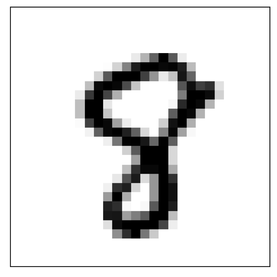
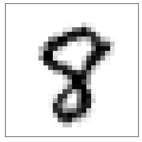
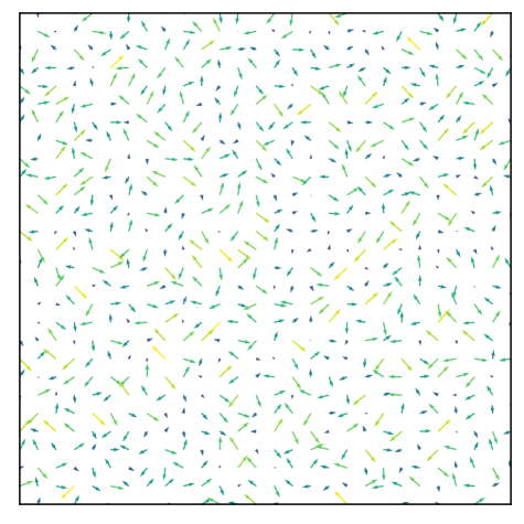
(a) label 8

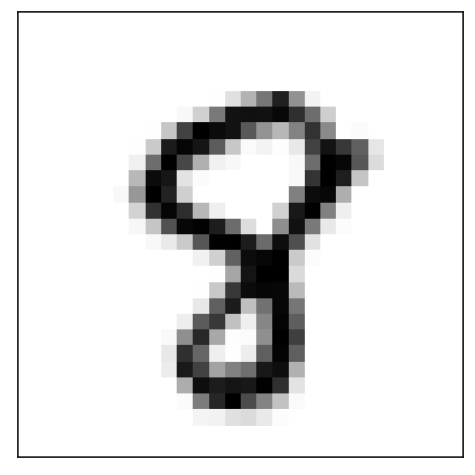
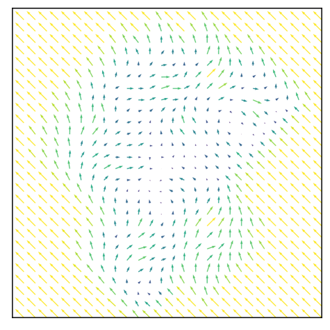
(b) label 8

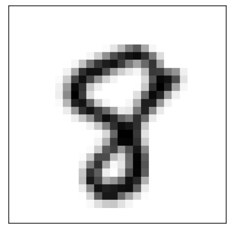
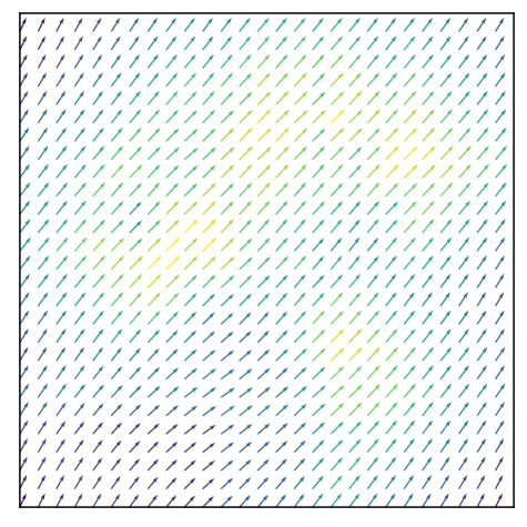
(c) label 8 (certified)

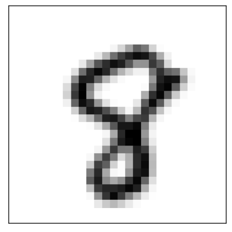
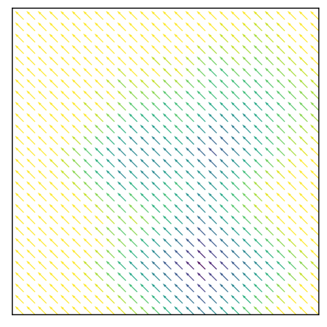
(d) label 8 (certified)

$\bm{\delta=0.4}$

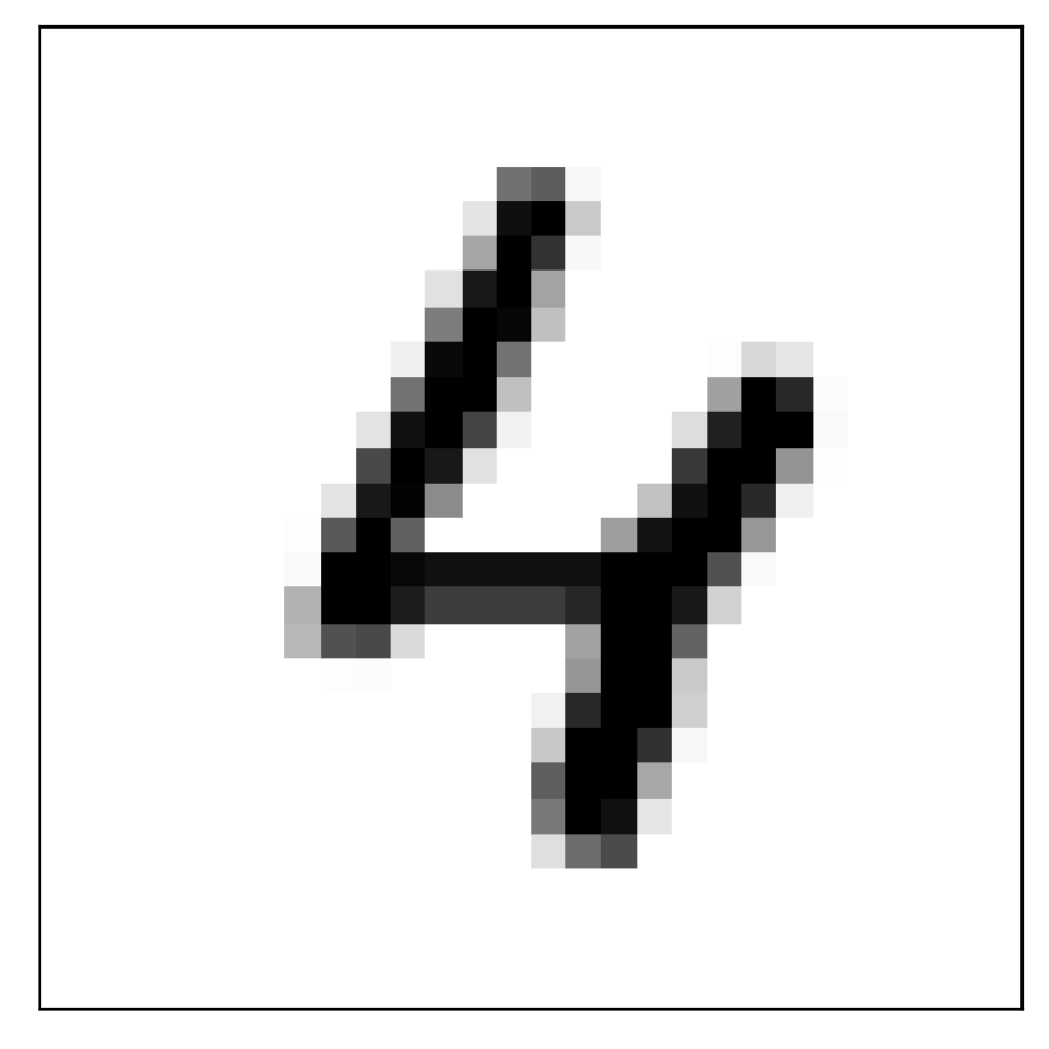
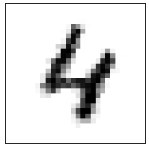
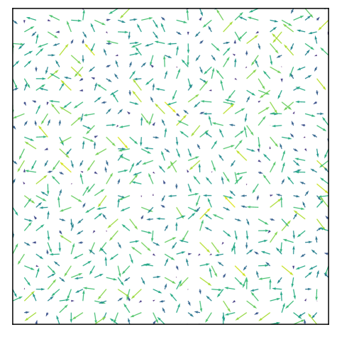
(e) label 5 (adversarial)

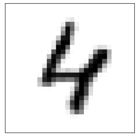
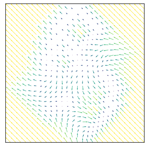
(f) label 4

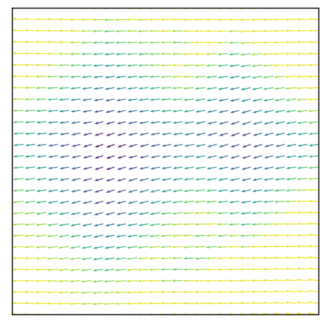
(g) label 4 (certified)

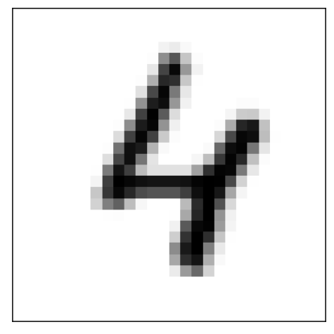
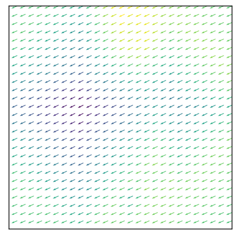
(h) label 4 (certified)

$\bm{\delta=0.5}$

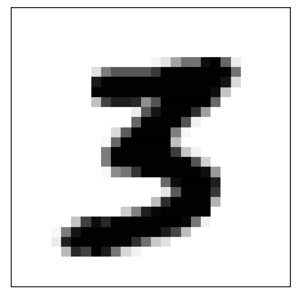
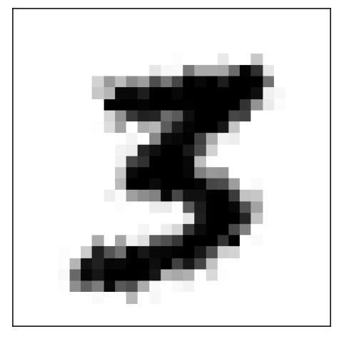
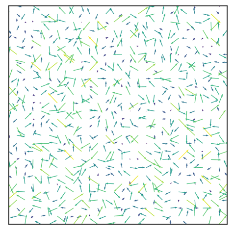
(i) label 5 (adversarial)

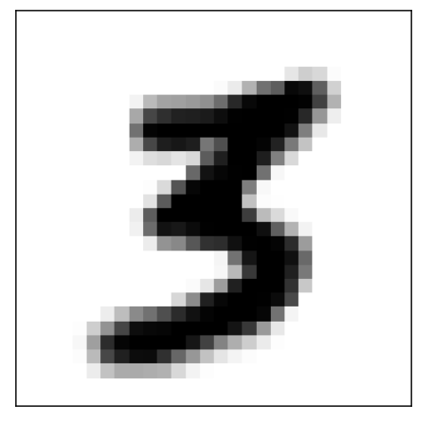
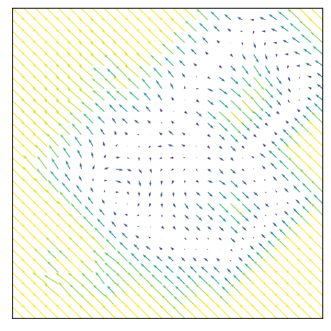
(j) label 9 (adversarial)

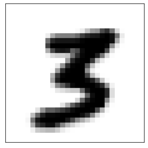
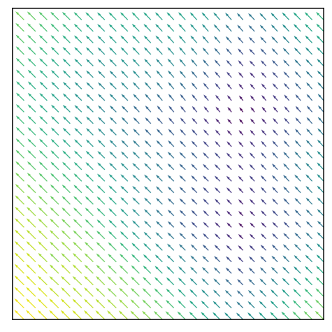
(k) label 3 (certified)

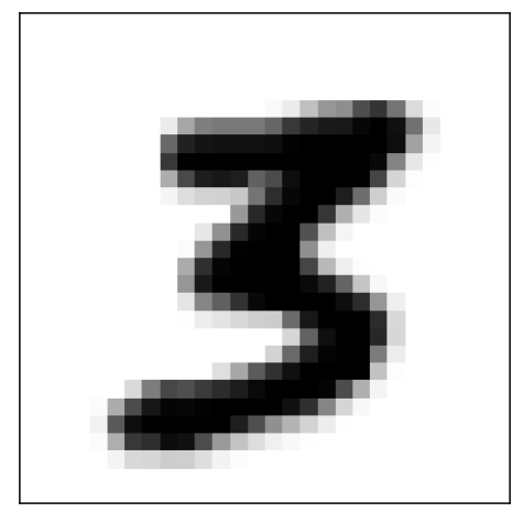
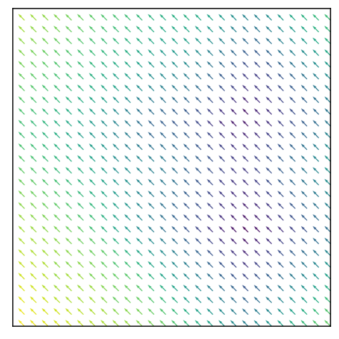
(l) label 3 (certified)

$\bm{\delta=0.6}$

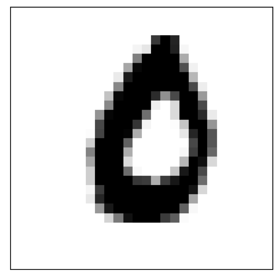
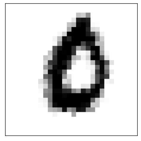
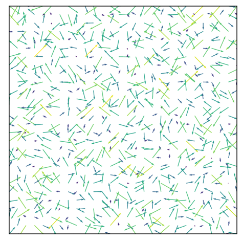
(m) label 4 (adversarial)

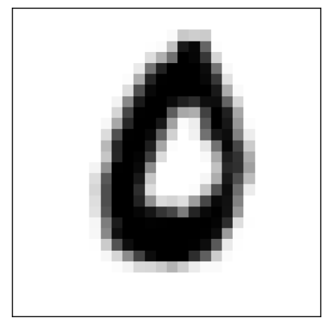
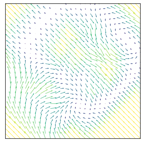
(n) label 0 (certified)

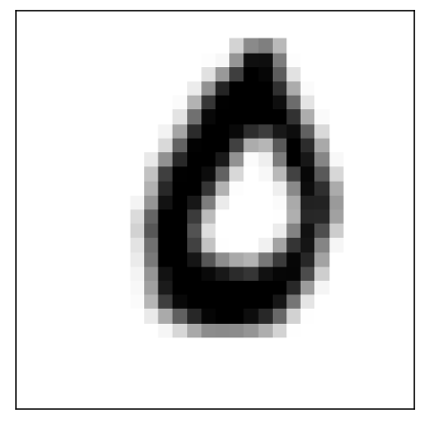
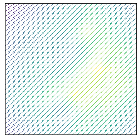
(o) label 0 (certified)

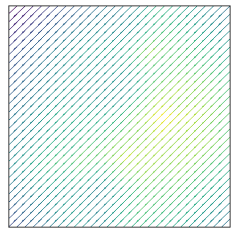
(p) label 0 (certified)

$\bm{\delta=0.7}$

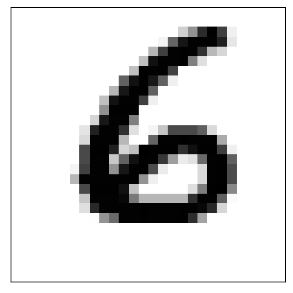
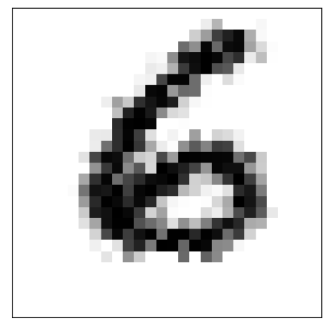
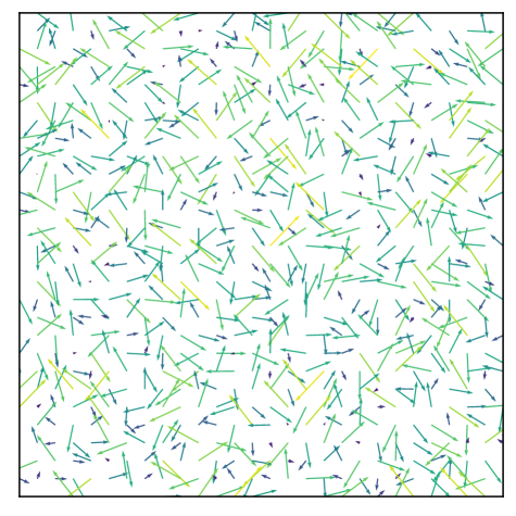
(q) label 6 (certified)

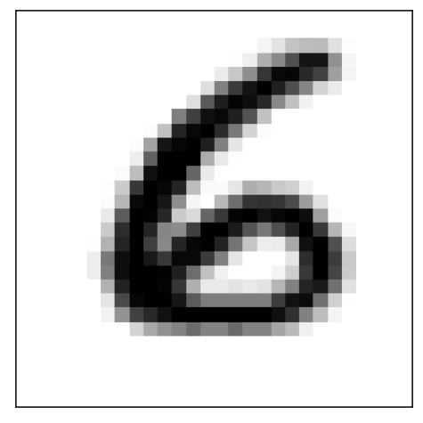
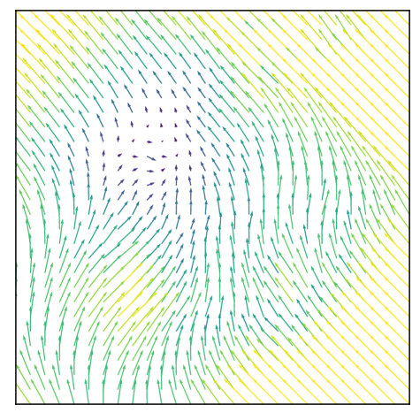
(r) label 6 (certified)

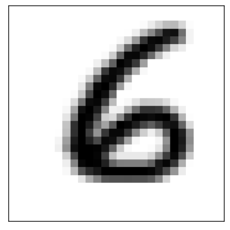
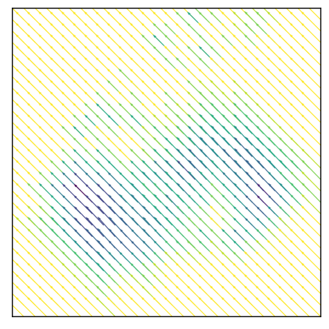
(s) label 6 (certified)

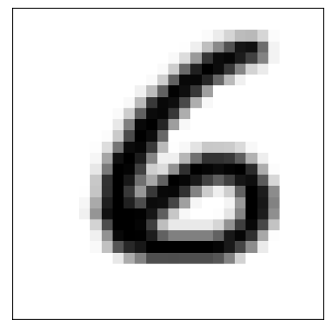
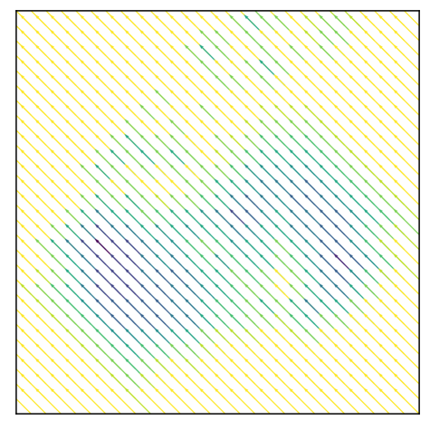
(t) label 6 (certified)

Figure 5: Image instances and corresponding deforming vector fields $\tau$ with displacement magnitude $\|\tau\|_{T_{\infty}}=\delta$ and flow $\gamma$.

	$T_{1}$-norm		$T_{2}$-norm		$T_{\infty}$-norm
$\delta$	DeepPoly	MILP	DeepPoly	MILP	DeepPoly	MILP
0.3	0.1	1.4	3.8	5.2	0.1	1.7
0.5	0.1	1.5	4.1	6.4	0.1	1.9
0.7	0.1	2.4	2.6	3.6	0.1	4.0
0.9	0.1	5.6	4.3	11.5	0.1	40.8

Table 5: Average running times (in seconds) for $T_{p}$-norm certification with $\gamma=\infty$ of ConvSmall DiffAI on MNIST.

Appendix D Visual Investigation

In this section, we compare original and deformed MNIST images for different $T_{\infty}$-norm values $\delta$ and flow-constraints $\gamma$. To that end, we employ the ConvSmall DiffAI network together with our convex relaxation with MILP to evaluate whether the deformed images are adversarial or certified (or neither) and we display the images in Figure 5. Note that since both MILP and our interval bounds are exact for single-channel images, the fact that Figure 5(a) is not adversarial is due to failure of the attack, as an adversarial vector field with $\delta=0.3$ and $\gamma=\infty$ must exist (else MILP would certify this image). On the other hand, for Figure 5(b) we cannot say whether the attacker fails to find an adversarial image or if our convex relaxation is not precise enough to certify the image (since we are using an over-approximation to enforce the flow-constraints).

References

- Alaifari, Alberti, and Gauksson (2019) Alaifari, R.; Alberti, G. S.; and Gauksson, T. 2019. ADef: an Iterative Algorithm to Construct Adversarial Deformations. In 7th International Conference on Learning Representations.
- Athalye and Carlini (2018) Athalye, A.; and Carlini, N. 2018. On the Robustness of the CVPR 2018 White-Box Adversarial Example Defenses. CoRR abs/1804.03286.
- Athalye, Carlini, and Wagner (2018) Athalye, A.; Carlini, N.; and Wagner, D. A. 2018. Obfuscated Gradients Give a False Sense of Security: Circumventing Defenses to Adversarial Examples. In Proceedings of the 35th International Conference on Machine Learning.
- Balunovic et al. (2019) Balunovic, M.; Baader, M.; Singh, G.; Gehr, T.; and Vechev, M. T. 2019. Certifying Geometric Robustness of Neural Networks. In Advances in Neural Information Processing Systems 32.
- Carlini and Wagner (2017) Carlini, N.; and Wagner, D. A. 2017. Towards Evaluating the Robustness of Neural Networks. In 2017 IEEE Symposium on Security and Privacy.
- Cohen, Rosenfeld, and Kolter (2019) Cohen, J. M.; Rosenfeld, E.; and Kolter, J. Z. 2019. Certified Adversarial Robustness via Randomized Smoothing. In Proceedings of the 36th International Conference on Machine Learning.
- Deng et al. (2009) Deng, J.; Dong, W.; Socher, R.; Li, L.; Li, K.; and Li, F. 2009. ImageNet: A large-scale hierarchical image database. In 2009 IEEE Computer Society Conference on Computer Vision and Pattern Recognition.
- Engstrom, Ilyas, and Athalye (2018) Engstrom, L.; Ilyas, A.; and Athalye, A. 2018. Evaluating and Understanding the Robustness of Adversarial Logit Pairing. CoRR abs/1807.10272.
- Engstrom et al. (2019) Engstrom, L.; Tran, B.; Tsipras, D.; Schmidt, L.; and Madry, A. 2019. Exploring the Landscape of Spatial Robustness. In Proceedings of the 36th International Conference on Machine Learning.
- Fischer, Baader, and Vechev (2020) Fischer, M.; Baader, M.; and Vechev, M. T. 2020. Certified Defense to Image Transformations via Randomized Smoothing. In Advances in Neural Information Processing Systems 33.
- Gehr et al. (2018) Gehr, T.; Mirman, M.; Drachsler-Cohen, D.; Tsankov, P.; Chaudhuri, S.; and Vechev, M. T. 2018. AI2: Safety and Robustness Certification of Neural Networks with Abstract Interpretation. In 2018 IEEE Symposium on Security and Privacy.
- Goodfellow, Shlens, and Szegedy (2015) Goodfellow, I. J.; Shlens, J.; and Szegedy, C. 2015. Explaining and Harnessing Adversarial Examples. In 3rd International Conference on Learning Representations.
- Gowal et al. (2019) Gowal, S.; Dvijotham, K.; Stanforth, R.; Bunel, R.; Qin, C.; Uesato, J.; Arandjelovic, R.; Mann, T. A.; and Kohli, P. 2019. Scalable Verified Training for Provably Robust Image Classification. In 2019 IEEE/CVF International Conference on Computer Vision.
- He et al. (2016) He, K.; Zhang, X.; Ren, S.; and Sun, J. 2016. Deep Residual Learning for Image Recognition. In 2016 IEEE Conference on Computer Vision and Pattern Recognition.
- Hu et al. (2020) Hu, J. E.; Swaminathan, A.; Salman, H.; and Yang, G. 2020. Improved Image Wasserstein Attacks and Defenses. CoRR abs/2004.12478.
- Kanbak, Moosavi-Dezfooli, and Frossard (2018) Kanbak, C.; Moosavi-Dezfooli, S.; and Frossard, P. 2018. Geometric Robustness of Deep Networks: Analysis and Improvement. In 2018 IEEE Conference on Computer Vision and Pattern Recognition.
- Katz et al. (2017) Katz, G.; Barrett, C. W.; Dill, D. L.; Julian, K.; and Kochenderfer, M. J. 2017. Reluplex: An Efficient SMT Solver for Verifying Deep Neural Networks. In Computer Aided Verification - 29th International Conference.
- Kerner (1966) Kerner, I. O. 1966. Ein Gesamtschrittverfahren zur Berechnung der Nullstellen von Polynomen. Numerische Mathematik 8.
- Krizhevsky (2009) Krizhevsky, A. 2009. Learning Multiple Layers of Features from Tiny Images. Master’s thesis, University of Toronto.
- LeCun, Cortes, and Burges (2010) LeCun, Y.; Cortes, C.; and Burges, C. 2010. MNIST handwritten digit database. ATT Labs [Online]. Available: http://yann.lecun.com/exdb/mnist 2.
- Lécuyer et al. (2019) Lécuyer, M.; Atlidakis, V.; Geambasu, R.; Hsu, D.; and Jana, S. 2019. Certified Robustness to Adversarial Examples with Differential Privacy. In 2019 IEEE Symposium on Security and Privacy.
- Levine and Feizi (2020) Levine, A.; and Feizi, S. 2020. Wasserstein Smoothing: Certified Robustness against Wasserstein Adversarial Attacks. In The 23rd International Conference on Artificial Intelligence and Statistics.
- Li et al. (2020) Li, L.; Weber, M.; Xu, X.; Rimanic, L.; Xie, T.; Zhang, C.; and Li, B. 2020. Provable Robust Learning Based on Transformation-Specific Smoothing. CoRR abs/2002.12398.
- Lin et al. (2019) Lin, W.; Yang, Z.; Chen, X.; Zhao, Q.; Li, X.; Liu, Z.; and He, J. 2019. Robustness Verification of Classification Deep Neural Networks via Linear Programming. In IEEE Conference on Computer Vision and Pattern Recognition.
- Madry et al. (2018) Madry, A.; Makelov, A.; Schmidt, L.; Tsipras, D.; and Vladu, A. 2018. Towards Deep Learning Models Resistant to Adversarial Attacks. In 6th International Conference on Learning Representations.
- Mirman, Gehr, and Vechev (2018) Mirman, M.; Gehr, T.; and Vechev, M. T. 2018. Differentiable Abstract Interpretation for Provably Robust Neural Networks. In Proceedings of the 35th International Conference on Machine Learning.
- Mohapatra et al. (2020) Mohapatra, J.; Weng, T.; Chen, P.; Liu, S.; and Daniel, L. 2020. Towards Verifying Robustness of Neural Networks Against A Family of Semantic Perturbations. In 2020 IEEE/CVF Conference on Computer Vision and Pattern Recognition.
- Pei et al. (2017) Pei, K.; Cao, Y.; Yang, J.; and Jana, S. 2017. Towards Practical Verification of Machine Learning: The Case of Computer Vision Systems. CoRR abs/1712.01785.
- Raghunathan, Steinhardt, and Liang (2018) Raghunathan, A.; Steinhardt, J.; and Liang, P. 2018. Semidefinite relaxations for certifying robustness to adversarial examples. In Advances in Neural Information Processing Systems 31.
- Salman et al. (2019a) Salman, H.; Li, J.; Razenshteyn, I. P.; Zhang, P.; Zhang, H.; Bubeck, S.; and Yang, G. 2019a. Provably Robust Deep Learning via Adversarially Trained Smoothed Classifiers. In Advances in Neural Information Processing Systems 32.
- Salman et al. (2019b) Salman, H.; Yang, G.; Zhang, H.; Hsieh, C.; and Zhang, P. 2019b. A Convex Relaxation Barrier to Tight Robustness Verification of Neural Networks. In Advances in Neural Information Processing Systems 32.
- Shmakov (2011) Shmakov, S. L. 2011. A Universal Method of Solving Quartic Equations. International Journal of Pure and Applied Mathematics 71.
- Singh et al. (2019a) Singh, G.; Ganvir, R.; Püschel, M.; and Vechev, M. T. 2019a. Beyond the Single Neuron Convex Barrier for Neural Network Certification. In Advances in Neural Information Processing Systems 32.
- Singh et al. (2018) Singh, G.; Gehr, T.; Mirman, M.; Püschel, M.; and Vechev, M. T. 2018. Fast and Effective Robustness Certification. In Advances in Neural Information Processing Systems 31.
- Singh et al. (2019b) Singh, G.; Gehr, T.; Püschel, M.; and Vechev, M. T. 2019b. An abstract domain for certifying neural networks. Proc. ACM Program. Lang. 3.
- Singh et al. (2019c) Singh, G.; Gehr, T.; Püschel, M.; and Vechev, M. T. 2019c. Boosting Robustness Certification of Neural Networks. In 7th International Conference on Learning Representations.
- Szegedy et al. (2014) Szegedy, C.; Zaremba, W.; Sutskever, I.; Bruna, J.; Erhan, D.; Goodfellow, I. J.; and Fergus, R. 2014. Intriguing properties of neural networks. In 2nd International Conference on Learning Representations.
- Tjeng, Xiao, and Tedrake (2019) Tjeng, V.; Xiao, K. Y.; and Tedrake, R. 2019. Evaluating Robustness of Neural Networks with Mixed Integer Programming. In 7th International Conference on Learning Representations.
- Tramèr et al. (2020) Tramèr, F.; Carlini, N.; Brendel, W.; and Madry, A. 2020. On Adaptive Attacks to Adversarial Example Defenses. In Advances in Neural Information Processing Systems 33.
- Wang et al. (2018) Wang, S.; Pei, K.; Whitehouse, J.; Yang, J.; and Jana, S. 2018. Efficient Formal Safety Analysis of Neural Networks. In Advances in Neural Information Processing Systems 31.
- Weng et al. (2018) Weng, T.; Zhang, H.; Chen, H.; Song, Z.; Hsieh, C.; Daniel, L.; Boning, D. S.; and Dhillon, I. S. 2018. Towards Fast Computation of Certified Robustness for ReLU Networks. In Proceedings of the 35th International Conference on Machine Learning.
- Wong and Kolter (2018) Wong, E.; and Kolter, J. Z. 2018. Provable Defenses against Adversarial Examples via the Convex Outer Adversarial Polytope. In Proceedings of the 35th International Conference on Machine Learning.
- Wong, Schmidt, and Kolter (2019) Wong, E.; Schmidt, F. R.; and Kolter, J. Z. 2019. Wasserstein Adversarial Examples via Projected Sinkhorn Iterations. In Proceedings of the 36th International Conference on Machine Learning.
- Wong et al. (2018) Wong, E.; Schmidt, F. R.; Metzen, J. H.; and Kolter, J. Z. 2018. Scaling provable adversarial defenses. In Advances in Neural Information Processing Systems 31.
- Wu and Kwiatkowska (2020) Wu, M.; and Kwiatkowska, M. 2020. Robustness Guarantees for Deep Neural Networks on Videos. In 2020 IEEE/CVF Conference on Computer Vision and Pattern Recognition.
- Xiao et al. (2018) Xiao, C.; Zhu, J.; Li, B.; He, W.; Liu, M.; and Song, D. 2018. Spatially Transformed Adversarial Examples. In 6th International Conference on Learning Representations.
- Zhang et al. (2018) Zhang, H.; Weng, T.; Chen, P.; Hsieh, C.; and Daniel, L. 2018. Efficient Neural Network Robustness Certification with General Activation Functions. In Advances in Neural Information Processing Systems 31.