Abstract

Deep Graph Neural Networks (GNNs) show promising performance on a range of graph tasks, yet at present are costly to run and lack many of the optimisations applied to DNNs. We show, for the first time, how to systematically quantise GNNs with minimal or no loss in performance using Network Architecture Search (NAS). We define the possible quantisation search space of GNNs. The proposed novel NAS mechanism, named Low Precision Graph NAS (LPGNAS), constrains both architecture and quantisation choices to be differentiable. LPGNAS learns the optimal architecture coupled with the best quantisation strategy for different components in the GNN automatically using back-propagation in a single search round. On eight different datasets, solving the task of classifying unseen nodes in a graph, LPGNAS generates quantised models with significant reductions in both model and buffer sizes but with similar accuracy to manually designed networks and other NAS results. In particular, on the Pubmed dataset, LPGNAS shows a better size-accuracy Pareto frontier compared to seven other manual and searched baselines, offering a $2.3\times$ reduction in model size but a $0.4\%$ increase in accuracy when compared to the best NAS competitor. Finally, from our collected quantisation statistics on a wide range of datasets, we suggest a W4A8 (4-bit weights, 8-bit activations) quantisation strategy might be the bottleneck for naive GNN quantisations.

1 Introduction

Graph Neural Networks (GNNs) have been successful in fields such as computational biology Zitnik & Leskovec (2017), social networks Hamilton et al. (2017), knowledge graphs Lin et al. (2015), etc.. The ability of GNNs to apply learned embeddings to unseen nodes or new subgraphs is useful for large scale machine learning systems on graph data, ranging from analysing posts on forums to creating product listings for shopping sites Hamilton et al. (2017). Most of the large production systems have high throughputs, running millions or billions of GNN inferences per second. This creates an urgent need to minimise both the computation and memory cost of GNN inference.

One common approach to reduce computation and memory overheads of Deep Neural Networks (DNNs) is quantisation Zhao et al. (2019); Zhang et al. (2018a); Hubara et al. (2016); Zhu et al. (2017); Hwang & Sung (2014). A simpler data format not only reduces the model size but also introduces the chance of using simpler arithmetic operations on existing or emerging hardware platforms Zhao et al. (2019); Hubara et al. (2016). Previous quantisation methods focusing solely on DNNs with image and sequence data will not obviously transfer well to GNNs. First, in CNNs and RNNs it is the convolutional and fully-connected layers that are quantised Hubara et al. (2016); Shen et al. (2019). GNNs, however, follow a sample and aggregate approach Zhao et al. (2020); Hamilton et al. (2017), where we can separate a basic building block in GNNs into four smaller sub-blocks (Linear, Attention, Aggregation and Activation); only a subset of these sub-blocks has trainable parameters and these parameters naturally have different precision requirements. Second, the design of GNN blocks involves a different design space, where several attention and aggregation methods are available and the choices of these methods have a direct interaction with the precision.

In this paper, we propose Low Precision Graph NAS (LPGNAS), which aims to automatically design quantised GNNs. The proposed NAS method is single-path, one-shot and gradient-based. Additionally, LPGNAS’s quantisation options are at a micro-architecture level so that different sub-blocks in a graph block can have different quantisation strategies. In this paper, we make the following contributions.

• To our knowledge, this is the first piece of work studying how to systematically quantise GNNs. We identify the quantisable components and possible search space for GNN quantisation.

• We present a novel single-path, one-shot and gradient-based NAS algorithm (LPGNAS) for automatically finding low precision GNNs.

• We report LPGNAS results, and show how they significantly outperfrom previous state-of-the-art NAS methods and manually designed networks in terms of memory consumption on the same accuracy budget on 8 different datasets.

• By running LPGNAS on a wide range of datasets, we reveal the quantisation statistics and show empirically LPGNAS converges to a 4-bit weights 8-bit activation fixed-point quantisation strategy. We further show this quantisation is the limitation of current fixed-point quantisation strategies on manually designed and searched GNNs.

2 Related Work

2.1 Quantisation and Network Architecture Search

DNNs offer great performance and rapid time-to-market path on a broad variety of tasks. Unfortunately, their high memory and computation requirements can be challenging when deploying in real-world scenarios. Quantisation directly shrinks model sizes and rapidly simplifies the complexity of the arithmetic hardware. Previous research shows that DNN models can be quantised to surprisingly low precisions such as ternary Zhu et al. (2017) and binary Hubara et al. (2016). Networks with extremely low precision weights have a significant task accuracy drop due to the numerical errors introduced, and sometimes require architectural changes to compensate Hubara et al. (2016). In contrast, fixed-point numbers Shen et al. (2019); Hwang & Sung (2014) and other more complex arithmetics Zhao et al. (2019); Zhang et al. (2018a) have larger bitwidths but offer a better task accuracy. These quantisation methods have primarily been applied on convolutional and fully-connected layers since they are the most compute-intensive building blocks in CNNs and RNNs. Another way of reducing the inference cost of DNNs is architectural engineering. For instance, using depth-wise separable convolutions to replace normal convolutions not only costs fewer parameters but also achieves comparable accuracy Howard et al. (2017). However, architectural engineering is normally tedious and complex; recent research on NAS reduces the amount of manual tuning in the architecture design process. Initial NAS methods used evolutionary algorithms and reinforcement learning to find optimal network architectures, but each iteration of the search fully trains and evaluates many child networks Real et al. (2017); Zoph & Le (2017), thus needing a huge amount of computation resources and time. Liu et al. proposed Differentiable Architecture Search (DARTs) that creates a supernet with all possible operations connected by probabilistic priors Liu et al. (2019). The search cost of DARTs is reduced by orders of magnitude – it is the same as training a single supernet (one-shot). In addition, DARTs is gradient-based, meaning that standard Stochastic Gradient Descent (SGD) now can be used to update these probabilistic priors. One major drawback of DARTs is that all operations of the supernet are active during the search. Recently proposed single-path NAS methods only update a sampled network from the supernet at each search step, and are able to converge quickly and significantly reduce the computation and memory cost compared to DARTs Wu et al. (2019); Cai et al. (2018); Guo et al. (2019). In addition, many of the NAS methods on vision networks consider mixed quantisation in their search space Guo et al. (2019); Wu et al. (2018), but limit the quantisation granularity to per-convolution level.

2.2 Graph Neural Network

Deep Learning on graphs has emerged into an important field of machine learning in recent years, partially due to the increase in the amount of graph-structured data. Graph Neural Networks has scored success in a range of different tasks on graph data, such as node classification Veličković et al. (2018); Kipf & Welling (2016); Hamilton et al. (2017), graph classification Zhang et al. (2018c); Ying et al. (2018); Xu et al. (2019) and link prediction Zhang & Chen (2018). There are many variants of graph neural networks proposed to tackle graph structured data. In this work we focus on GNNs applied to node classification tasks based on Message-Passing Neural Networks (MPNN) Gilmer et al. (2017). The objective of the neural network is to learn an embedding function for node features so that they quickly generalise to other unseen nodes. This inductive nature is needed for large-scale production level machine learning systems, since they normally operate on a constantly changing graph with many coming unseen nodes (e.g. shopping history on Amazon, posts on Reddit etc.) Hamilton et al. (2017). It is also worth to mention that many of these systems are high-throughput and latency-critical. The reductions in energy and latency of the deployed networks imply the service providers can offer a better user experience while keeping a lower cost.

Most of the manually designed GNN architectures proposed for the node classification use MPNN. The list includes, but is not limited to, GCN Kipf & Welling (2016), GAT Veličković et al. (2018), GraphSage Hamilton et al. (2017), and their variants Shi et al. (2019); Zhang et al. (2018b); Chen et al. (2017); Wang et al. (2019). These works differ in ways of computing the edge weights, sampling neighbourhood and aggregating neighbour messages. We also relate to works focusing on building deeper Graph Neural Networks with the help of residual connections, such as JKNet Xu et al. (2018). To the best of our knowledge, there is no prior work in investigating quantisation for Graph Neural Networks.

There is a recent surge of interest in looking at how to extend NAS methods from image and sequence data to graphs. Gao et al. proposed GraphNAS that is a RL-based NAS applied to graph data Gao et al. (2019). Later, Zhou et al. combined the RL-based NAS with parameter sharing Zhou et al. (2019) and developed AutoGNN. Zhao et al.  proposed a gradient-based, single-shot NAS called PDNAS, and searched both the micro- and macro-architectures of GNNs Zhao et al. (2020). All of these graph NAS methods show superior performance when compared to other manually designed networks.

Table 1: Quantisation search space for weights and activations.

Weights Activations Quantisation Frac Bits Total Bits Quantisation Frac Bits Total Bits binary 0 1 fix$2.2$ 2 4 binary 0 1 fix$4.4$ 4 8 ternary 0 2 fix$2.2$ 2 4 ternary 0 2 fix$4.4$ 4 8 ternary 0 2 fix$4.8$ 4 12 fix$1.3$ 3 4 fix$4.4$ 4 8 fix$2.2$ 2 4 fix$4.4$ 4 8 fix$1.5$ 5 6 fix$4.4$ 4 8 fix$3.3$ 3 6 fix$4.4$ 4 8 fix$2.4$ 4 6 fix$4.4$ 4 8 fix$4.4$ 4 8 fix$4.4$ 4 8 fix$4.4$ 4 8 fix$4.8$ 8 12 fix$4.4$ 4 8 fix$8.8$ 8 16 fix$4.8$ 8 12 fix$4.8$ 8 12 fix$4.12$ 12 16 fix$4.4$ 4 8 fix$4.12$ 12 16 fix$4.8$ 8 12 fix$4.12$ 12 16 fix$8.8$ 8 16

3 Method

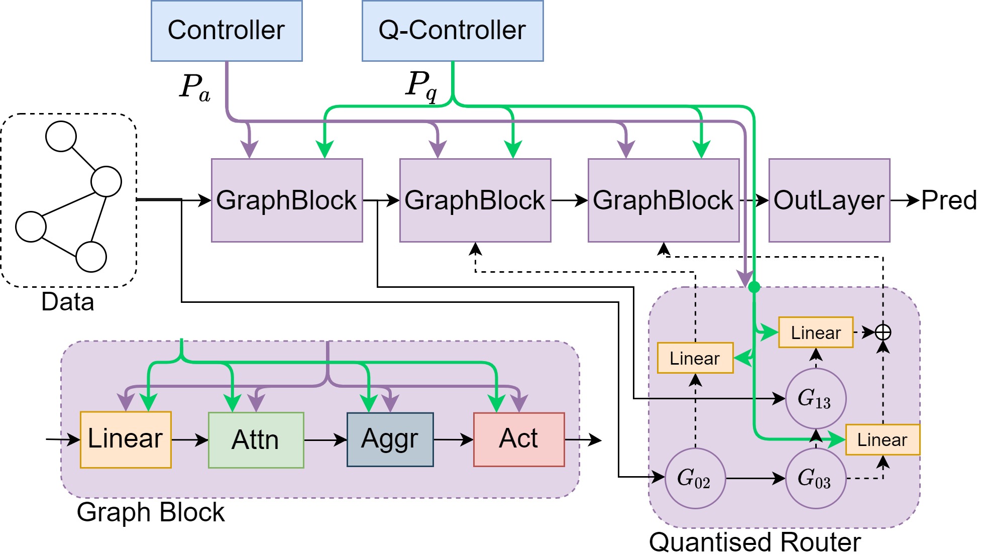
Figure 1: An overview of the LPGNAS architecture. $P_{a}$ denotes controller output (Purple) for selecting different operations within each graph block, and for routing shortcut connections between graph blocks. $P_{q}$ denotes quantisation controller (Q-Controller) output (Green) for selecting quantisations for operations within graph blocks and shortcut connections. $G_{ij}$ are gating functions conditioned on $P_{a}$. Solid lines are input streams into the router while dashed lines are output streams.

3.1 Quantisation Search Space

Table 2: Different types of attention mechanisms. $W$ here is parameter vector for attention. $<,>$ is dot product, $a_{ij}$ is attention for message from node $j$ to node $i$.

Attention Type	Equation
Const	$a_{ij}=1$
GCN	$a_{ij}=\frac{1}{\sqrt{d_{i}d_{j}}}$
GAT	$a^{gat}_{ij}=\mathsf{LeakyReLU}(W_{a}(h_{i}||h_{j}))$
Sym-GAT	$a_{ij}=a^{gat}_{ij}+a^{gat}_{ji}$
COS	$a_{ij}=<W_{a1}h_{i},W_{a2}h_{j}>$
Linear	$a_{ij}=\mathsf{tanh}(\sum_{j\in N(i)}(W_{a}h_{j}))$
Gene-Linear	$a_{ij}=W_{g}\mathsf{tanh}(W_{a1}h_{i}+W_{a2}h_{j})$

Table 3: Different types of activation functions.

Activation	Equation
None	$f(x)=x$
Sigmoid	$f(x)=\frac{1}{1+e^{-x}}$
Tanh	$f(x)=tanh(x)$
Softplus	$f(x)=\frac{1}{\beta}\log(1+e^{\beta x})$
ReLU	$f(x)=Max(0,x)$
LeakyReLU	$f(x)=Max(0,x)+\alpha Min(0,x)$
ReLU6	$f(x)=Min(Max(0,x),6)$
ELU	$f(x)=Max(0,x)+Min(0,\alpha(e^{x}-1))$

We consider a single graph block, or a GNN layer, as four consecutive sub-blocks (Equation 1). Equation 1 considers node features $h^{k-1}$ from the $k-1$ layer as inputs, and produces new node features $h^{k}$ with trainable attention parameters $a^{k}$ and weights $w^{k}$. The four sub-blocks, as illustrated in Equation 1, are the Linear block, Attention block, Aggregation block and Activation block; these sub-blocks have operations as search candidates, which is a similar architectural search space to Zhao et al. Zhao et al. (2020) and Gao et al. Gao et al. (2019). We provide a detailed description of the architectural search space in the Appendix. In Equation 2, we label all possible quantisation candidates using $Q$. The quantisation function $Q$ can be applied not only on learnable parameters (e.g., $w^{k}$) but also activation values between consecutive sub-blocks. In addition, we allow quantisation options in Equation 2 to be different. For instance, ${\color[rgb]{0,0,1}Q_{a}}$ can learn to have a different quantisation from ${\color[rgb]{0,0,1}Q_{w}}$, meaning that a single graph block receives a mixed quantisation for different quantisable components annotated in Equation 2.

$$h^{k}=\mathsf{Act}(\mathsf{Aggr}(\mathsf{Atten}(a^{k},\mathsf{Linear}(w^{k},h^{k-1}))))$$ (1)

$$\begin{split}h^{k}_{\mathsf{linear}}&={\color[rgb]{0,0,1}Q_{l}(}\mathsf{Linear}({\color[rgb]{0,0,1}Q_{w}(}w^{k}{\color[rgb]{0,0,1})},{\color[rgb]{0,0,1}Q_{h}(}h^{k-1}{\color[rgb]{0,0,1})}){\color[rgb]{0,0,1})}\\ h^{k}_{\mathsf{atten}}&={\color[rgb]{0,0,1}Q_{at}(}\mathsf{Atten}({\color[rgb]{0,0,1}Q_{a}(}a^{k}{\color[rgb]{0,0,1})},h^{k}_{\mathsf{linear}}){\color[rgb]{0,0,1})}\\ h^{k}&=\mathsf{Act}({\color[rgb]{0,0,1}Q_{ag}(}\mathsf{Aggr}(h^{k}_{\mathsf{atten}}){\color[rgb]{0,0,1})})\\ \end{split}$$ (2)

The reasons for considering input activation values as quantisation candidates are the following. First, GNNs always consider large input graph data, the computation operates on a per-node or per-edge resolution but requires the entire graph or the entire sampled graph as inputs. The amount of intermediate data produced during the computation is huge and causes a large pressure on the amount of on-chip memory available. Second, quantised input activations with quantised parameters together simplify the arithmetic operations. For instance, $\mathsf{Linear}({\color[rgb]{0,0,1}Q_{w}(}w^{k}{\color[rgb]{0,0,1})},{\color[rgb]{0,0,1}Q_{h}(}h^{k-1}{\color[rgb]{0,0,1})}){\color[rgb]{0,0,1})})$ considers both quantised $h^{k-1}$ and quantised $w^{k}$ so that the matrix multiplication with these values can operate on a simpler fixed-point arithmetic.

The quantisation search space identified in Equation 2 is different from the search space identified by Wu et al. Wu et al. (2018) and Guo et al. Guo et al. (2019). Most existing NAS methods focusing on quantising CNNs look at quantisation at each convolutional block. In our case, a single graph block is equivalent to a convolutional block and we look at more fine-grained quantisation opportunities within the four sub-blocks. The quantisation search considers a wide range of fixed-point quantisations. The weights and activation can pick the numbers of bits in $[1,2,4,6,8,12,16]$ and $[4,8,12,16]$ respectively, and we allow different integer and fractional bits combinations We list the detailed quantisation options in the Table 1. Table 1 shows the quantisation search space, each quantisable operation identified will have these quantisation choices available. BINARY means binary quantisation, and TERNARY means two-bit tenary quantiation. FIX$x.y$ means fixed-point quantisation with $x$ integer bits and $y$ bits for fractions.

In total, as listed in Table 1, we have $17$ quantisation options; and as illustrated in Equation 2, there are four sub-blocks that join the quantisation search, this gives us in total $17^{4}=83251$ quantisation options.

3.2 Architecture Search Space

As illustrated in Figure 1, each graph block consists of four sub-blocks, namely the linear block, attention block, aggregation block and activation block. Each of these sub-blocks contain architectural choices that joins the NAS process. In Table 2 and Table 3, we list all attention types and activation types that were considered in the architectural search space. We also consider searching for the best hidden feature size, using two fully-connected layers with an intermediate layer with an expansion factor that can be picked from a set $\{1,2,4,8\}$. The possible aggregation choices include $mean$, $add$ and $max$.

The considered search space is similar to prior works in this domain Zhao et al. (2020); Zhou et al. (2019); Gao et al. (2019). The possible number of architectural combinations of a single layer is $7\times 8\times 3\times 4=672$, for an $n$-layer network, this means there are in total $672^{n}$ possible architectural combinations. Combining the quantisation search space mentioned in the previous section, the search space has in total $83251\times 672^{n}$ options. Assuming the number of layers considered in the search is $n=4$, this roughly gives us a search space of $10^{15}$ options.

3.3 Low Precision Graph Network Architecture Search

Algorithm 1 LPGNAS algorithm

  Input: $x$, $y$, $x_{v}$, $y_{v}$, $M$, $M_{a}$, $M_{q}$, $K$, $\alpha$, $\beta$

  $\mathsf{Init}(w,w_{a},w_{q})$

  for $i=0$ to $M-1$ do

     $N$ = NoiseGen($i$, $\alpha$)

     $P_{a},P_{q}$ = $g_{a}(w_{a},x_{\mathsf{val}},N),g_{q}(w_{q},x_{\mathsf{val}},N)$

     $\pi_{a},\pi_{q}=\operatorname*{arg\,max}(P_{a}),\operatorname*{arg\,max}(P_{q})$

     for $i=0$ to $K-1$ do

        $\mathcal{L}=\mathsf{Loss}(x,y,\pi_{a},\pi_{q})$

        $w$ = $\mathsf{Opt}_{w}(\mathcal{L})$

     end for

     $\mathcal{L}_{v}=\mathsf{Loss}(x_{v},y_{v},\pi_{a},\pi_{q})$

     if $e>M_{a}$ then

        $w_{a}$ = $\mathsf{Opt}_{w_{a}}(\mathcal{L}_{v})$

     end if

     if $e>M_{q}$ then

        $\mathcal{L}_{q}=\mathsf{QLoss}(P_{a},P_{q})$

        $w_{q}$ = $\mathsf{Opt}_{w_{q}}(\mathcal{L}_{v}+\beta L_{q})$

     end if

  end for

We describe the Low Precision Graph Network Architecture Search (LPGNAS) algorithm in Algorithm 1. ($x$, $y$), ($x_{v}$, $x_{v}$) are the training and validation data respectively. $M$ is the total number of search epochs, and $M_{a}$ and $M_{q}$ are the epochs to start architectural and quantisation search. Similar to Zhao et al. Zhao et al. (2020), before the number of epochs reaches $M_{a}$ or $M_{q}$, LPGNAS randomly picks up samples and warms up the trainable parameters in the supernet. $K$ is the number of steps to iterate in training the supernet. After generating noise $N$, we use this noise in architectural controller $g_{a}$ and quantisation controller $g_{q}$ together with the validation data $x_{v}$ to determine the architectural $\pi_{a}$ and quantisation $\pi_{q}$ choices. After reaching the pre-defined starting epoch ($M_{a}$ or $M_{q}$), LPGNAS starts to optimise the controllers’ weights ($w_{a}$ and $w_{q}$). We choose the hyper-parameters $M_{q}=20,M_{a}=50,\alpha=1.0,\beta=0.1$, unless specified otherwise, based on the choices made by Zhao et al. Zhao et al. (2020). In addition, we provide an ablation study in the Appendix to justify our choices of hyper-parameters. Notice that $\mathsf{QLoss}$ estimates the current hardware cost based on both architectural and quantisation probabilities. As shown in Equation 3, we define $S$ as a set of values that represents the costs (number of parameters) of all possible architectural options: for each value $s$ in this set, we multiply it with the probability $p_{a}$ from architecture probabilities $P_{a}$ generated by the NAS architecture controller. Similarly, we produce the weighted-sum for quantisation from the set of values $S_{q}$ that represents costs of all possible quantisations. The dot product $\cdot$ between these two weighted-sum vectors produces the quantisation loss $L_{q}$.

$$\begin{split}L_{q}&=\mathsf{QLoss}(P_{a},P_{q})\\ &=\sum_{s\in S,p_{a}\in P_{a}}(s*p_{a})\cdot\sum_{s_{q}\in S_{q},p_{q}\in P_{q}}(s_{q}*p_{q})\end{split}$$ (3)

Figure 1 is an illustration of the LPGNAS algorithm. We use two controllers ($g_{a}$ and $g_{q}$) for architecture and quantisation (named as Controller and Q-Controller in the diagram) respectively. The controllers use trainable embeddings connected to linear layers to produce architecture and quantisation probabilities. The architecture controller provides probabilities ($P_{a}$) for picking architectural options of graph blocks and also the router. The router is in charge of determining how each graph block shortcuts to the subsequent graph blocks Zhao et al. (2020). In addition, the quantisation controller provides quantisation probabilities ($P_{q}$) to both modules in graph blocks and the linear layers in the router. In a graph block, only the linear and attention layers have quantisable parameters and have matrix multiplication operations; neither activation nor aggregation layers have any trainable or quantisable parameters. However, all input activation values of each layer in the graph block are quantised. The amount of intermediate data produced during the computation causes memory pressure on many existing or emerging hardware devices, so even for modules that do not have quantisable parameters, we choose to quantise their input activation values to help reduce the amount of buffer space required.

4 Results

Table 4: Accuracy and size comparison on Cora, Pubmed and Citeseer with data splits same as Yang et al. (2016). Our results are averaged across 3 independent runs. The numbers in bold show best accuracies or smallest sizes.

Method Quan Cora CiteSeer PubMed Accuracy Size Accuracy Size Accuracy Size GraphSage float $74.5\pm 0.0\%$ $92.3$KB $75.3\pm 0.0\%$ $237.5$KB $85.3\pm 0.1\%$ $32.2$KB GraphSage w10a12 $74.3\pm 0.1\%$ $28.8$KB $75.1\pm 0.1\%$ $74.2$KB $85.0\pm 0.0\%$ $10.1$KB GAT float $88.9\pm 0.0\%$ $369.5$KB $75.9\pm 0.0\%$ $950.3$KB $86.1\pm 0.0\%$ $129.6$KB GAT w4a8 $88.8\pm 0.1\%$ $46.2$KB $68.0\pm 0.1\%$ $118.8$KB $82.0\pm 0.0\%$ $16.2$KB JKNet float $88.7\pm 0.0\%$ $214.9$KB $75.5\pm 0.0\%$ $505.2$KB $87.6\pm 0.0\%$ $94.5$KB JKNet w6a8 $88.7\pm 0.1\%$ $\mathbf{40.3}$KB $73.2\pm 0.1\%$ $94.7$KB $86.1\pm 0.1\%$ $17.7$KB PDNAS-2 float $89.3\pm 0.1\%$ $192.2$KB $\mathbf{76.3\pm 0.3\%}$ $478.6$KB $89.1\pm 0.2\%$ $72.8$KB PDNAS-3 float $89.3\pm 0.1\%$ $200.0$KB $75.5\pm 0.3\%$ $494.4$KB $89.1\pm 0.2\%$ $81.4$KB PDNAS-4 float $89.8\pm 0.3\%$ $205.0$KB $75.6\pm 0.2\%$ $500.0$KB $89.2\pm 0.1\%$ $102.7$KB LPGNAS mixed $\mathbf{89.8\pm 0.0\%}$ $67.3$KB $76.2\pm 0.1\%$ $\mathbf{56.5}$KB $\mathbf{89.6\pm 0.1\%}$ $45.6$KB

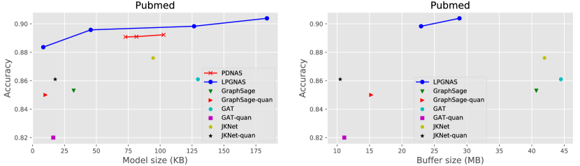
Figure 2: Pareto Frontier of LPGNAS and PDNAS Zhao et al. (2020) on the Pubmed datset Yang et al. (2016), the manually designed networks are shown as dots. On the left, we show the trade-off between model sizes and accuracy; on the right, the trade-off is between buffer sizes and accuracy.

We compare LPGNAS to both manually designed and searched GNNs. In addition, we provide comparisons for two types of tasks. The first type is on the Citation datasets, where the network takes the entire graph as an input in a transductive learning setup Yang et al. (2016). The second type considers inputs sampled from a large graph, and we use the inductive GraphSAINT sampling strategy Zeng et al. (2020). For the networks to learn from sampled graphs, we present results on larger datasets, including Amazon Computers, Amazon Photos Shchur et al. (2018), Yelp, Flickr Zeng et al. (2020) and Cora-full Bojchevski & Günnemann (2017).

Table 5: Accuracy and size comparison on Amazon-Computers and Amazon-Photo Shchur et al. (2018) Our results are averaged across 3 independent runs. The numbers in bold show best accuracies (blue) and smallest model sizes (red).

Method Quan Amazon-Computers Amazon-Photos Accuracy Size Accuracy Size GAT float $84.4\pm 0.3\%$ 199.8KB $84.2\pm 0.1\%$ 199.8KB GAT w4a8 $81.8\pm 1.5\%$ 25.0KB $83.5\pm 0.5\%$ 25.0KB GAT-V2 float $85.3\pm 0.3\%$ 1597.6KB $85.2\pm 0.4\%$ 1597.6KB GAT-V2 w4a8 $38.0\pm 0.0\%$ 199.7KB $38.0\pm 0.0\%$ 199.7KB JKNet float $87.6\pm 0.0\%$ 130.5KB $87.7\pm 0.1\%$ 130.5KB JKNet w4a8 $38.0\pm 0.0\%$ 16.3KB $38.0\pm 0.0\%$ 16.3KB JKNet-V2 float $88.8\pm 0.1\%$ 8968.2KB $88.6\pm 0.1\%$ 8968.2KB QJKNet-V2 w4a8 $38.0\pm 0.0\%$ 1121.0KB $38.0\pm 0.0\%$ 1121.0KB SageNet float $84.0\pm 0.0\%$ 49.8KB $84.0\pm 0.1\%$ 49.8KB SageNet w4a8 $83.9\pm 0.1\%$ 6.2KB $83.9\pm 0.1\%$ 6.2KB SageNet-V2 float $87.7\pm 0.2\%$ 1593.4KB $87.9\pm 0.2\%$ 1593.4KB SageNet-V2 w4a8 $87.3\pm 0.2\%$ 199.2KB $87.2\pm 0.3\%$ 199.2KB LPGNAS mixed $\mathbf{90.5\pm 0.0}\%$ 157.3KB $\mathbf{89.7\pm 0.0}\%$ 164.0KB LPGNAS-small mixed $88.7\pm 0.1\%$ $\mathbf{3.5}$KB $88.6\pm 0.1\%$ $\mathbf{3.6}$KB

Table 6: Accuracy and size comparison on Flickr Zeng et al. (2020), Cora-full Bojchevski & Günnemann (2017) and Yelp Zeng et al. (2020). Our results are averaged across 3 independent runs. The numbers in bold show best accuracies (blue) and smallest model sizes (red).

Method Quan Flickr CoraFull Yelp Accuracy Size Accuracy Size Micro-F1 Size GAT float $42.4\pm 0.1\%$ 130.6KB $62.0\pm 0.1\%$ 2249.3KB $24.6\pm 0.5\%$ 104.4KB QGAT w4a8 $42.4\pm 0.0\%$ 16.3KB $53.8\pm 0.2\%$ 281.2KB $14.2\pm 0.0\%$ 13.0KB GAT-V2 float $44.6\pm 0.9\%$ 1044.6KB $65.5\pm 0.3\%$ 17988.4KB $32.0\pm 0.0\%$ 826.5KB QGAT-V2 w4a8 $42.3\pm 0.0\%$ 130.6KB $4.4\pm 0.0\%$ 2248.6KB $14.2\pm 0.0\%$ 103.3KB JKNet float $50.6\pm 0.0\%$ 95.5KB $69.0\pm 0.1\%$ 1162.8KB $32.6\pm 0.3\%$ 94.1KB QJKNet w4a8 $42.3\pm 0.0\%$ 11.9KB $4.4\pm 0.0\%$ 145.3KB $31.0\pm 2.2\%$ 11.8KB JKNet-V2 float $50.2\pm 0.2\%$ 8409.1KB $68.7\pm 0.1\%$ 25481.5KB $33.1\pm 1.6\%$ 8380.8KB QJKNet-V2 w4a8 $42.3\pm 0.0\%$ 1051.1KB $4.4\pm 0.0\%$ 3185.2KB $14.2\pm 0.0\%$ 1047.6KB SageNet float $49.9\pm 0.0\%$ 32.5KB $66.4\pm 0.1\%$ 562.3KB $23.6\pm 0.0\%$ 26.1KB QSageNet float $45.0\pm 0.0\%$ 4.1KB $65.7\pm 0.2\%$ 70.3KB $24.8\pm 0.0\%$ 3.3KB SageNet-V2 float $50.0\pm 0.0\%$ 1040.4KB $68.2\pm 0.0\%$ 17983.8KB $30.5\pm 0.6\%$ 821.6KB QSageNet-V2 w4a8 $49.7\pm 0.3\%$ 130.1KB $68.4\pm 0.3\%$ 2248.0KB $27.4\pm 0.7\%$ 102.7KB LPGNAS mixed $\mathbf{73.4\pm 0.0}\%$ 81.2KB $\mathbf{85.5\pm 0.0}\%$ 432.3KB $\mathbf{40.5\pm 0.1}\%$ 6.4KB LPGNAS-small mixed $70.6\pm 0.1\%$ $\mathbf{2.2}$KB $80.2\pm 0.1\%$ $\mathbf{70.2}$KB $30.9\pm 0.1\%$ $\mathbf{1.5}$KB

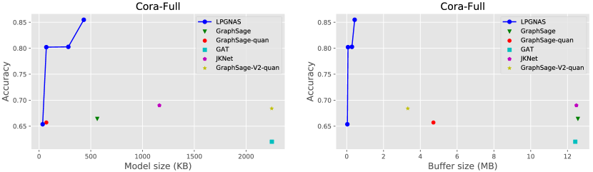
Figure 3: Pareto Frontier of LPGNAS and other baselines on the Cora-full dataset Yang et al. (2016), the manually designed networks are shown as dots. On the left, we show the trade-off between model sizes and accuracy; on the right, the trade-off is between buffer sizes and accuracy.

The Citation datasets include nodes representing documents and edges representing citation links. The task is to distinguish which research field the document belongs to Yang et al. (2016). The Flickr dataset includes nodes as images, and edges exist between two images if they share some common properties. The task is to classify these images based on their bag-of-words encoded features Zeng et al. (2020). Yelp considers users as nodes and edges are made based on user friendships, and features are word embeddings extracted from user reviews. The task is to distinguish the categories of the shops the users are likely to review; since multiple categories are possible, the labels are multi-hot Zeng et al. (2020). Amazon Computers and Photo are part of the Amazon co-purchase graph McAuley et al. (2015). The nodes are goods, and edges are the frequency between two goods bought together. Node features are bag-of-words encoded product reviews, and classes are the product categories. Cora-full is an extended version of Cora, which one of the dataset in the Citation datasets. We provide a detailed overview of the properties and statistics of the datasets in Appendix.

4.1 Citation Datasets

Table 4 shows the performance of GraphSage Hamilton et al. (2017), GAT Veličković et al. (2018), JKNet Xu et al. (2018), PDNAS Zhao et al. (2020) and LPGNAS on the citation datasets with a partition of $0.6$, $0.2$, $0.2$ for training, validation and testing respectively, which is the same training setup as in Yang et al. Yang et al. (2016). For the quantisation options of GraphSage, GAT and JKNet, we manually perform a grid search on the Cora dataset. The grid search considers various weight and activation quantisations in a decreasing order. The search terminates when quantisation causes a decrease in accuracy bigger than $0.5\%$ and rolls back to pick the previous quantisation applied as the result. We reimplemented GraphSage Hamilton et al. (2017), GAT Veličković et al. (2018) and JKNet Xu et al. (2018) for quantisation, and provide the architecture choices and details of the grid search in the Appendix. For the manual baseline networks, we used the quantisation strategy found on Cora for Citeseer and Pubmed. For LPGNAS, we searched with a set of base configurations that we clarified in the Appendix. For all reimplemented baselines, we train the networks with three different seeds and report the averaged results with standard deviations. For LPGNAS, we run the entire search and train cycle three times and report the final averaged accuracy trained on the searched network.

The results in Table 4 suggest that LPGNAS shows better accuracy on both Cora and Pubmed with quantised networks. In addition, although LPGNAS does not show the smallest sizes on these two datasets, it is only slightly bigger than the manual baselines but shows a much better accuracy. On Citeseer, LPGNAS only shows slightly worse accuracy (around $0.1\%$ less) with a considerably smaller size (around $9\times$ reduction in model sizes).

To further prove the point that LPGNAS generates more efficient networks, we sweep across different configurations and different quantisation regularisations to produce Figure 2 to visulise the performance of LPGNAS and how it performs with small model sizes. We explain in the Appendix how this sweep of different LPGNAS configurations work, the sweep mainly considers a combination of different configurations of how many layers and how many base channel counts are there for the backbone network to use for LPGNAS. We plot the Pareto frontiers of LPGNAS putting model sizes on the horizontal axis and accuracy on the vertical axis for Pubmed (Figure 2). In this plot, we also demonstrate how buffer size trades-off with accuracy. For buffer size, it means the total size required to hold all intermediate activation values during the computation of a single inference run with a batch size of one. GNNs normally use large graphs as input data; the amount of memory required to hold all intermediate values might be a limiting factor in batched inference. Since LPGNAS uses quantisation not only on weights but also on input activation values, it shows a better trade-off than the floating-point baselines. For Figure 2, models staying at the top left of the plots are considered as better, since they are consuming less hardware resources and maintaining high accuracy. In addition, in Figure 2, we compare PDNAS Zhao et al. (2020) to LPGNAS and found that we outperformed the floating-point NAS methods by staying at the top left in the plot.

Table 7: Search cost in GPU hours, all experiments are conducted on an NVIDIA GeForce RTX 2080 Ti GPU.

Dataset Cora Citeseer Pubmed Cora-full Flickr Yelp Amazon-photos Amazon-computers LPGNAS 3.2 3.6 4.2 11.8 11.0 11.8 11.4 11.2 JKNet-32 6518.5 8165.6 5289.1 2180.6 3062.1 9116.7 1739.8 1786.2

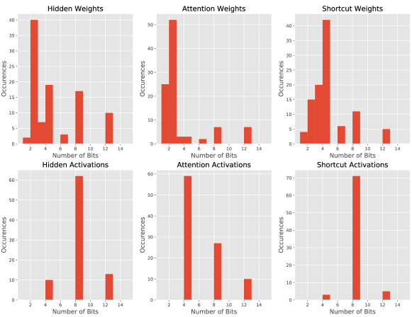
Figure 4: Collected statistical information for quantisation, the horizontal axis shows the chosen bitwidth and the vertical axis shows the occurences. A bitwith count of 16 is not present because it has never been selected by LPGNAS.

4.2 Graph Sampling Based Learning

Table 5 and Table 6 show how LPGNAS performs on large datasets sampled using the GraphSaint sampling Zeng et al. (2020). The detailed configuration of the sampler is in the Appendix. We provide additional baselines on these datasets since the original GraphSage Hamilton et al. (2017), GAT Veličković et al. (2018), JKNet Xu et al. (2018) underfit this challenging task. We thus implemented V2 versions of the baselines that have larger channel counts; the architecture details are reported in our Appendix. In addition, for quantising the baseline models we uniformly applied a w4a8 (4-bit weights, 8-bit input activations) quantisation. Although we train on a sampled sub-graph, evaluating networks requires a full traversal of the complete graph. Since the datasets considered are large, traversing the entire graph adds a huge computation overhead. If we use the previous grid-search for all quantisation possibilities (roughly $16^{4}$ in our case) for the all baseline networks, this will require a huge amount of search time. So we fixed our quantisation strategy to w4a8 for the baseline networks.

The results in Table 5 and Table 6 suggest that LPGNAS found the models with best accuracy and also with a relatively competitive model size when compared to a wide range of manual baselines. To further demonstrate that LPGNAS is a flexible NAS method, we adjust the base configurations to provide models that are equal or smaller than the smallest baseline networks in Table 5 and Table 6 and name them LPGNAS-small. We describe how we turn the knobs in LPGNAS by adjusting the base configurations in our Appendix. It is clear, in both Table 5 and Table 6, that LPGNAS outperforms all baselines in terms of accuracy or micro-F1 scores. LPGNAS-small, on the other hand, trades-off the accuracy for a better model size, however it shows better performance than baseline models that have a similar size budget.

We also visualise the performance of LPGNAS on sampled datasets using the Pareto frontiers plot for Cora-full in Figure 3. As expected, LPGNAS shows a frontier at the top left, proving that it is able to produce small networks with high accuracy values. In other words, LPGNAS is Pareto dominated compared other manually designed networks.

It is worth to note that LPGNAS show great performance gains compared to the baseline networks. On Flickr, CoraFull, and Yelp, we show on average around $20\%$ increase compared to even the full-precision baseline models, while our LPGNAS produced quantised models. The performance gap between quantised baselines and LPGNAS is even greater. On the other hand, LPGNAS is able to produce extremely small models. For instance, LPGNAS-Small is able to produce models that are around $50\times$ smaller on Amazon-Computers and Amazon-Photos while only suffer from an around $1\%$ drop in accuracy compared to standard LPGNAS.

4.3 Quantisation Search Time

One advantage of using Network Architecture Search is the reduction of search time. Previous NAS methods on GNNs demonstrated the effectiveness of their methods by reducing the amount of search time required to find the best network architecture Zhao et al. (2020); Gao et al. (2019); Zhou et al. (2019). In this work, we not only reduced the amount of manual tunning time required for network architectures but also shortened the amount of time required to search for numerical precisions at different sub-blocks.

To further illustrate that LPGNAS has significantly reduced the amount of search time required, we provide Table 7 to show how LPGNAS compares to a fixed JKNet-32 architecture in terms of the amount of GPU hours spent for searching for the best quantisation options. Because of the limited resources we have, we estimate the quantisation search cost of a JKNet-32 by running 5 different randomly selected quantisation combinations and multiply the averaged training time with the total number of quantisation options.

Table 7 shows that LPGNAS can significantly reduce the search time. For instance, on Citeseer, the search time can be reduced by around $2270\times$. It is worth noting that, when performing this quantisation search time comparison, we do not consider the architectural search space of the baseline, meaning that the baseline (JKNet) is a fixed-architecture. LPGNAS also searched for architecture choices, which would further increases the search time of the baseline if they are considered.

4.4 Quantisation Statistics and Limitations

In order to fully understand the properties of different quantisable sub-blocks in GNNs, we report the searched quantisation strategies on more than 100 search runs across 8 different datasets (Cora, Pubmed, Citeseer, Amazon-Computers, Amazon-Photos, Flickr, CoraFull and Yelp). The idea is to reveal some common quantisation properties or trends using LPGNAS on different datasets. We collect the quantisation decisions made by LPGNAS for both weights and activations and present them in Figure 4. The possible quantisation levels for weights and activations are [1, 2, 4, 6, 8, 12, 16] and [4, 8, 12, 16] bits respectively.

For weights, most quantisation choices tend to use small bitwidths: binary and ternary values seem to be sufficient for the hidden and attention sub-blocks, however, shortcut connections prefer a larger bitwidth (around 4 bits) for weights. In contrast, quantising activations show in general a trend of using larger bitwidths (around 8 bits). Based on these results, if one would like to manually quantise GNNs, we would suggest to start with around 4 bits for weights and 8 bits for activations. However, it is worth mentioning that LPGNAS might trade quantisation choices with architectural decisions. For instance, we observed LPGNAS was able to choose operations with less parameters but use higher bitwidths. Nevertheless, the large number of runs across a relatively wide range of datasets aim at sharing empirical insights for people that are manually tuning quantisations for GNNs. For GNN services that are whether energy, memory or latency critical, and for future AI ASIC designers focusing on GNN inference, the gathered quantisation statistics can be a useful guideline for fitting a suitable quantisation method to their networks.

It is also interesting to observe that in both Table 5 and Table 6, some of the manually designed GNNs suffer from a large accuracy drop when applying a 4-bit weight and 8-bit activation fixed-point quantisation (w4a8). For instance, both quantised JKNet and JKNet-V2 drop down to $4.4\%$ accuracy on the Cora-full dataset (Table 5). However, the collected statistics of LPGNAS suggest that w4a8 is sufficient, proving that modifications of network architectures are the key element for networks to maintain accuracy with aggressive quantisation strategies.

The applied fixed-point quantisation is a straight-forward one, many researchers have proposed more advanced quantisation schemes on CNNs or RNNs Zhao et al. (2019); Zhang et al. (2018a); Shin et al. (2016). We suggest future research of investigating how these quantisation strategies work on GNNs should consider w4a8 fixed-point quantisation as a baseline case. Because our collected statistics suggest that w4a8 fixed-point quantisation is the most aggressive quantisation for searched GNNs while guaranteeing minimal loss of accuracy, and manual GNNs often do not perform well using the w4a8 setup.

5 Conclusion

In this paper, we propose a novel single-path, one-shot and gradient-based NAS algorithm named LPGNAS. LPGNAS is able to generate compact quantized networks with state-of-the-art accuracy. To our knowledge, this is the first piece of work studying the quantisation of GNNs. We define the GNN quantisation search space and show how it can be co-optimised with the original architectural search space. In addition, we empirically show the limitation of GNN quantisation using the proposed NAS algorithm, most of the searched networks converge to a 4-bit weight 8-bit activation quantisation setup. Despite this limitation, LPGNAS demonstrates superior performance when compared to networks generated manually or by other NAS methods on a wide range of datasets.

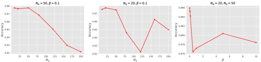
Figure 5: Collected statistical information for quantisation, the horizontal axis shows the chosen bitwidth and the vertical axis shows the occurences.

Appendix A Parameter Choices

As mentioned in the LPGNAS algorithm, we pick $N_{q}=20,N_{a}=50,\alpha=1.0,\beta=0.1,\mathsf{lr}=0.005$. The values of $\alpha$ and $\mathsf{lr}$ are the same as Zhao et al. Zhao et al. (2020). For $\beta$, $N_{q}$ and $N_{a}$, we justify our choices in Figure 5 by sweeping across different values of $\beta$, $N_{a}$ and $N_{q}$ on the Pubmed dataset.

Appendix B Datasets Information and Data Sampler Configurations

In this section we decribe in details the dataset we used. In our experiments we use dataset preprocessing and loading implementations from Pytorch Geometric Fey & Lenssen (2019).

Citation Dataset: Citation dataset Yang et al. (2016) is a standard benchmark dataset for graph learning. It comprises three publication datasets, which are Cora, CiteSeer and PubMed. There is an additional extended version of Cora called Cora-Full Bojchevski & Günnemann (2017). Cora contains all Machine Learning papers in the Cora-Full graph. In these datasets, nodes correspond to bag-of-word features of the documents and edges indicates citation. Each node has a class label. In this paper we use the 6:2:2 train/validation/test split ratio.

Amazon Dataset: Amazon datasets Shchur et al. (2018), including Amazon Photos and Amazon Computers, are segments of the Amazon co-purchase graph. Nodes represent goods while edges represent frequent co-purchase of linked goods. Node feature is bag-of-word features of product review, while node label is its category. We use the 6:2:2 train/validation/test split ratio.

Flickr and Yelp Dataset: Flickr and Yelp datasets are introduced along GraphSAINT Zeng et al. (2020). In Flickr dataset, nodes represent images uploaded to Flickr, and edges represent sharing of common properties (e.g. location and comments by same user). Node feature is 500-dimensional bag-of-words representation based on SIFT descpritions, and node label is its class. In Yelp dataset, nodes represent users and edges represent friendship between users. Node feature is summed word2vec embeddings of words in the user’s reviews, and node label is a multi-hot vector representing which types of businesses has the user reviewed. For both dataset we use the 6:2:2 train/validation/test split ratio.

Appendix C Grid Search and Baseline Networks Details

For producing quantised baseline networks, we manually grid searched options listed in Table 1 and follow the order from bottom to top. We stop the search and retrieve to the previous quantisation stage if the current stage shows an accuracy drop of more than $0.5\%$. It is worth to mention this grid search for quantisation is very time-consuming, and we therefore only performed on Cora and used the found quantisation strategy for the rest of the Citation datasets.

Table 8 shows the configurations of the baseline networks we’ve used in this paper.

Table 8: Baseline networks configurations.

Networks Layers Channels GAT 2 32 GAT-V2 2 64 JKNet 2 32 JKNet-V2 2 512 SageNet 2 16 SageNet-V2 2 512

References

- Bojchevski & Günnemann (2017) Bojchevski, A. and Günnemann, S. Deep gaussian embedding of graphs: Unsupervised inductive learning via ranking. arXiv preprint arXiv:1707.03815, 2017.
- Cai et al. (2018) Cai, H., Zhu, L., and Han, S. Proxylessnas: Direct neural architecture search on target task and hardware. arXiv preprint arXiv:1812.00332, 2018.
- Chen et al. (2017) Chen, J., Zhu, J., and Song, L. Stochastic training of graph convolutional networks with variance reduction. arXiv preprint arXiv:1710.10568, 2017.
- Fey & Lenssen (2019) Fey, M. and Lenssen, J. E. Fast graph representation learning with PyTorch Geometric. In ICLR Workshop on Representation Learning on Graphs and Manifolds, 2019.
- Gao et al. (2019) Gao, Y., Yang, H., Zhang, P., Zhou, C., and Hu, Y. GraphNAS: Graph neural architecture search with reinforcement learning. arXiv preprint arXiv:1904.09981, 2019.
- Gilmer et al. (2017) Gilmer, J., Schoenholz, S. S., Riley, P. F., Vinyals, O., and Dahl, G. E. Neural message passing for quantum chemistry. In Proceedings of the 34th International Conference on Machine Learning-Volume 70, pp. 1263–1272. JMLR. org, 2017.
- Guo et al. (2019) Guo, Z., Zhang, X., Mu, H., Heng, W., Liu, Z., Wei, Y., and Sun, J. Single path one-shot neural architecture search with uniform sampling. arXiv preprint arXiv:1904.00420, 2019.
- Hamilton et al. (2017) Hamilton, W., Ying, Z., and Leskovec, J. Inductive representation learning on large graphs. In Advances in Neural Information Processing Systems, pp. 1024–1034, 2017.
- Howard et al. (2017) Howard, A. G., Zhu, M., Chen, B., Kalenichenko, D., Wang, W., Weyand, T., Andreetto, M., and Adam, H. Mobilenets: Efficient convolutional neural networks for mobile vision applications. arXiv preprint arXiv:1704.04861, 2017.
- Hubara et al. (2016) Hubara, I., Courbariaux, M., Soudry, D., El-Yaniv, R., and Bengio, Y. Binarized neural networks. In Advances in neural information processing systems, pp. 4107–4115, 2016.
- Hwang & Sung (2014) Hwang, K. and Sung, W. Fixed-point feedforward deep neural network design using weights , , and . In Signal Processing Systems, 2014.
- Kipf & Welling (2016) Kipf, T. N. and Welling, M. Semi-supervised classification with graph convolutional networks. arXiv preprint arXiv:1609.02907, 2016.
- Lin et al. (2015) Lin, Y., Liu, Z., Sun, M., Liu, Y., and Zhu, X. Learning entity and relation embeddings for knowledge graph completion. In Twenty-ninth AAAI conference on artificial intelligence, 2015.
- Liu et al. (2019) Liu, H., Simonyan, K., and Yang, Y. DARTS: Differentiable architecture search. In International Conference on Learning Representations, 2019. URL https://openreview.net/forum?id=S1eYHoC5FX.
- McAuley et al. (2015) McAuley, J., Targett, C., Shi, Q., and Van Den Hengel, A. Image-based recommendations on styles and substitutes. In Proceedings of the 38th International ACM SIGIR Conference on Research and Development in Information Retrieval, pp. 43–52, 2015.
- Real et al. (2017) Real, E., Moore, S., Selle, A., Saxena, S., Suematsu, Y. L., Tan, J., Le, Q. V., and Kurakin, A. Large-scale evolution of image classifiers. In Proceedings of the 34th International Conference on Machine Learning-Volume 70, pp. 2902–2911. JMLR. org, 2017.
- Shchur et al. (2018) Shchur, O., Mumme, M., Bojchevski, A., and Günnemann, S. Pitfalls of graph neural network evaluation. arXiv preprint arXiv:1811.05868, 2018.
- Shen et al. (2019) Shen, S., Dong, Z., Ye, J., Ma, L., Yao, Z., Gholami, A., Mahoney, M. W., and Keutzer, K. Q-bert: Hessian based ultra low precision quantization of bert. arXiv preprint arXiv:1909.05840, 2019.
- Shi et al. (2019) Shi, L., Zhang, Y., Cheng, J., and Lu, H. Two-stream adaptive graph convolutional networks for skeleton-based action recognition. In Proceedings of the IEEE Conference on Computer Vision and Pattern Recognition, pp. 12026–12035, 2019.
- Shin et al. (2016) Shin, S., Hwang, K., and Sung, W. Fixed-point performance analysis of recurrent neural networks. In 2016 IEEE International Conference on Acoustics, Speech and Signal Processing (ICASSP), pp. 976–980. IEEE, 2016.
- Veličković et al. (2018) Veličković, P., Cucurull, G., Casanova, A., Romero, A., Liò, P., and Bengio, Y. Graph Attention Networks. International Conference on Learning Representations, 2018. URL https://openreview.net/forum?id=rJXMpikCZ.
- Wang et al. (2019) Wang, X., Ji, H., Shi, C., Wang, B., Ye, Y., Cui, P., and Yu, P. S. Heterogeneous graph attention network. In The World Wide Web Conference, pp. 2022–2032, 2019.
- Wu et al. (2018) Wu, B., Wang, Y., Zhang, P., Tian, Y., Vajda, P., and Keutzer, K. Mixed precision quantization of convnets via differentiable neural architecture search. arXiv preprint arXiv:1812.00090, 2018.
- Wu et al. (2019) Wu, B., Dai, X., Zhang, P., Wang, Y., Sun, F., Wu, Y., Tian, Y., Vajda, P., Jia, Y., and Keutzer, K. FBNET: Hardware-aware efficient convnet design via differentiable neural architecture search. In Proceedings of the IEEE Conference on Computer Vision and Pattern Recognition, pp. 10734–10742, 2019.
- Xu et al. (2018) Xu, K., Li, C., Tian, Y., Sonobe, T., Kawarabayashi, K.-i., and Jegelka, S. Representation learning on graphs with jumping knowledge networks. In International Conference on Machine Learning, pp. 5449–5458, 2018.
- Xu et al. (2019) Xu, K., Hu, W., Leskovec, J., and Jegelka, S. How powerful are graph neural networks? In International Conference on Learning Representations, 2019. URL https://openreview.net/forum?id=ryGs6iA5Km.
- Yang et al. (2016) Yang, Z., Cohen, W. W., and Salakhutdinov, R. Revisiting semi-supervised learning with graph embeddings. In Proceedings of the 33rd International Conference on International Conference on Machine Learning-Volume 48, pp. 40–48. JMLR. org, 2016.
- Ying et al. (2018) Ying, Z., You, J., Morris, C., Ren, X., Hamilton, W., and Leskovec, J. Hierarchical graph representation learning with differentiable pooling. In Advances in neural information processing systems, pp. 4800–4810, 2018.
- Zeng et al. (2020) Zeng, H., Zhou, H., Srivastava, A., Kannan, R., and Prasanna, V. GraphSAINT: Graph sampling based inductive learning method. In International Conference on Learning Representations, 2020. URL https://openreview.net/forum?id=BJe8pkHFwS.
- Zhang et al. (2018a) Zhang, D., Yang, J., Ye, D., and Hua, G. LQ-Nets: Learned quantization for highly accurate and compact deep neural networks. In European Conference on Computer Vision (ECCV), 2018a.
- Zhang et al. (2018b) Zhang, J., Shi, X., Xie, J., Ma, H., King, I., and Yeung, D.-Y. Gaan: Gated attention networks for learning on large and spatiotemporal graphs. arXiv preprint arXiv:1803.07294, 2018b.
- Zhang & Chen (2018) Zhang, M. and Chen, Y. Link prediction based on graph neural networks. In Advances in Neural Information Processing Systems, pp. 5165–5175, 2018.
- Zhang et al. (2018c) Zhang, M., Cui, Z., Neumann, M., and Chen, Y. An end-to-end deep learning architecture for graph classification. In Thirty-Second AAAI Conference on Artificial Intelligence, 2018c.
- Zhao et al. (2019) Zhao, Y., Gao, X., Bates, D., Mullins, R., and Xu, C.-Z. Focused quantization for sparse cnns. In Advances in Neural Information Processing Systems, pp. 5585–5594, 2019.
- Zhao et al. (2020) Zhao, Y., Wang, D., Gao, X., Mullins, R., Lio, P., and Jamnik, M. Probabilistic dual network architecture search on graphs. arXiv preprint arXiv:2003.09676, 2020.
- Zhou et al. (2019) Zhou, K., Song, Q., Huang, X., and Hu, X. Auto-GNN: Neural architecture search of graph neural networks. arXiv preprint arXiv:1909.03184, 2019.
- Zhu et al. (2017) Zhu, C., Han, S., Mao, H., and Dally, W. J. Trained ternary quantization. International Conference on Learning Representations (ICLR), 2017.
- Zitnik & Leskovec (2017) Zitnik, M. and Leskovec, J. Predicting multicellular function through multi-layer tissue networks. Bioinformatics, 33(14):i190–i198, 2017.
- Zoph & Le (2017) Zoph, B. and Le, Q. V. Neural architecture search with reinforcement learning. 2017.