Population Susceptibility Variation and Its Effect on Contagion Dynamics

Abstract

Susceptibility governs the dynamics of contagion. The classical SIR model is one of the simplest compartmental models of contagion spread, assuming a single shared susceptibility level. However, variation in susceptibility over a population can fundamentally alter the dynamics of contagion and thus the ultimate outcome of a pandemic. We develop mathematical machinery which explicitly considers susceptibility variation, illuminates how the susceptibility distribution is sculpted by contagion, and thence how such variation affects the SIR differential questions that govern contagion. Our methods allow us to derive closed form expressions for herd immunity thresholds as a function of initial susceptibility distributions and suggests an intuitively satisfying approach to inoculation when only a fraction of the population is accessible to such intervention. Of particular interest, if we assume static susceptibility of individuals in the susceptible pool, ignoring susceptibility diversity always results in overestimation of the herd immunity threshold and that difference can be dramatic. Therefore, we should develop robust measures of susceptibility variation as part of public health strategies for handling pandemics.

I Introduction

The differential equations typically used to describe contagion [1, 2] place the population into three different tranches:

• ${x_{S}}$: susceptible fraction/number

• ${x_{I}}$: infected fraction/number

• ${x_{R}}$: recovered fraction/number

Assuming the fractional form, we have

$${x_{S}}+{x_{I}}+{x_{R}}=1$$

There are also two key parameters governing contagion dynamics:

• $\beta$: the rate ($(\mbox{individual-time})^{-1}$) of transmission

• $\gamma$: the rate ($\mbox{time}^{-1}$) of recovery

which lead to the fundamental coupled differential equations of contagion

$${{\dot{x}_{S}}}=-\beta{x_{S}}{x_{I}}$$

and

$${{\dot{x}_{I}}}=\left(\beta{x_{S}}-\gamma\right){x_{I}}$$

However, all members of a population are not necessarily as susceptible to contagion as others [3, 4, 5]. So, let $\epsilon\geq 0$ be the susceptibility of an individual to a given disease. Small values of $\epsilon$ imply greater resistance, while large values imply greater susceptibility. We can then define the random variable ${\cal E}(t)$ as the susceptibility of an individual chosen randomly from the susceptible population at time $t$. Its probability density function is ${f_{{\cal E}{(t)}}}(\epsilon)$ and

$${F_{{\cal E}{(t)}}}(\epsilon)=\int_{0}^{\epsilon}{f_{{\cal E}{(t)}}}(x)dx$$

is its cumulative distribution function – the probability that an individual randomly selected from the population at time $t$ will have a susceptibility less than or equal to $\epsilon$.

Now consider a Gedankenexperiment where individuals are selected randomly from the population and exposed to contagion. Our key assumption is that

Individuals with susceptibility $\epsilon$ will be removed from the susceptible pool at a rate $\beta{{x_{I}}}\epsilon$.

Over time, such removals will alter the population susceptibility landscape ${f_{{\cal E}{(t)}}}(\epsilon)$. That is, individuals with higher susceptibility are preferentially removed early, and this process, repeated many times, will increase the relative proportion of less susceptible individuals. We seek to understand in general how ${f_{{\cal E}{(t)}}}(\epsilon)$ evolves in time. So we amend the equations of contagion as

$${{\dot{{x_{S}}}}}=-\beta{\bar{\cal E}}(t){x_{S}}{x_{I}}$$ (1)

and

$${{\dot{{x_{I}}}}}=\left(\beta{\bar{\cal E}}(t){x_{S}}-\gamma\right){x_{I}}$$ (2)

where ${\bar{\cal E}}(t)$ is the mean susceptibility of the population – which we take to be initially ${\bar{\cal E}}(0)=1$.

We will find that if the initial susceptibility distribution, ${f_{{\cal E}{(0)}}}(\epsilon)$ is Gamma-distributed, then ${f_{{\cal E}{(t)}}}(\epsilon)$ stays Gamma-distributed. However, we also find that the contagion process, if left to run long enough, tends to sculpt ${f_{{\cal E}{(0)}}}(\epsilon)$ into an approximation of a Gamma distribution. The exceptions include initial mixed (singular $+$ continuous) distributions as well as those with non-compact support. However, if the initial distribution can be expressed over its domain as a power series (including series representations with non-integer powers), then ${f_{{\cal E}{(t)}}}(\epsilon)$ approaches a Gamma distribution of some order. But most importantly, given the general assumptions of the SIR model and assuming static individual susceptibility we will find that

• Ignoring susceptibility diversity always results in overestimation of the herd immunity threshold.

• The population susceptibility distribution shape affects

  • the ultimate severity of contagion.

  • the effectiveness of mitigation techniques

II Evolution of ${f_{{\cal E}{(t)}}}(\epsilon)$

Taking a differential approach consider that for a small time-step ${\mbox{\small$\Delta$}t\,}$, the probability density ${f_{{\cal E}{(t+{\mbox{\small$\Delta$}t\,})}}}(\epsilon)$ must be

$${f_{{\cal E}{(t+{\mbox{\small$\Delta$}t\,})}}}(\epsilon) = \frac{\displaystyle{f_{{\cal E}{(t)}}}(\epsilon)(1-\beta{{x_{I}}}(t+{\mbox{\small$\Delta$}t\,}){\mbox{\small$\Delta$}t\,}\epsilon)}{\displaystyle\int{f_{{\cal E}{(t)}}}(\epsilon)\left(1-\beta{{x_{I}}}(t+{\mbox{\small$\Delta$}t\,}){\mbox{\small$\Delta$}t\,}\epsilon\right)d\epsilon}$$

$$= \frac{(1-\beta{{x_{I}}}(t+{\mbox{\small$\Delta$}t\,}){\mbox{\small$\Delta$}t\,}\epsilon)}{1-\beta{{x_{I}}}(t+{\mbox{\small$\Delta$}t\,}){\mbox{\small$\Delta$}t\,}{\bar{\cal E}}(t)}{f_{{\cal E}{(t)}}}(\epsilon)$$

We then have $\frac{{f_{{\cal E}{(t+{\mbox{\small$\Delta$}t\,})}}}(\epsilon)-{f_{{\cal E}{(t)}}}(\epsilon)}{{\mbox{\small$\Delta$}t\,}}$ as

$$\frac{\beta{{x_{I}}}(t+{\mbox{\small$\Delta$}t\,}){\mbox{\small$\Delta$}t\,}({\bar{\cal E}}(t)-\epsilon)}{{\mbox{\small$\Delta$}t\,}\left(1-\beta{{x_{I}}}(t+{\mbox{\small$\Delta$}t\,}){\mbox{\small$\Delta$}t\,}{\bar{\cal E}}(t)\right)}{f_{{\cal E}{(t)}}}(\epsilon)$$

which after ${\mbox{\small$\Delta$}t\,}$ disappears from numerator and denominator leaves

$$\frac{\beta{{x_{I}}}(t+{\mbox{\small$\Delta$}t\,})({\bar{\cal E}}(t)-\epsilon)}{1-\beta{{x_{I}}}(t+{\mbox{\small$\Delta$}t\,}){\mbox{\small$\Delta$}t\,}{\bar{\cal E}}(t)}{f_{{\cal E}{(t)}}}(\epsilon)$$

which as ${\mbox{\small$\Delta$}t\,}\rightarrow 0$ reduces to

$$\boxed{\frac{d}{dt}{f_{{\cal E}{(t)}}}(\epsilon)=\beta{{x_{I}}}({\bar{\cal E}}(t)-\epsilon){f_{{\cal E}{(t)}}}(\epsilon)}$$ (3)

Equation (3) is the differential equation governing the evolution of ${f_{{\cal E}{(t)}}}(\epsilon)$ in time under the action of contagion. We immediately see that susceptibility above average will be muted while susceptibility below average will be amplified. As equation (3) evolves, we will expect ${\bar{\cal E}}(t)$ to decrease and the probability mass of ${\cal E}(t)$ to become more and more concentrated around smaller values of susceptibility.

II-A A General Solution

We assume one individual’s susceptibility does not affect another’s. So, we can imagine a given susceptibility tranche as being exponentially diminished according to its susceptibility value $\epsilon$. If ${x_{S}}(\epsilon,0)$ is the size of that tranche at time zero, then we may expect

$${x_{S}}(\epsilon,t)\propto e^{-\beta{{{\cal X}_{I}}}\epsilon}{x_{S}}(\epsilon,0)$$ (4)

where we define

$${{{\cal X}_{I}}}=\int_{0}^{t}{{x_{I}}}dt$$ (5)

as the cumulative ”infection pressure.” We note that so long as ${{x_{I}}}$ does not contain singularities, ${{{\cal X}_{I}}}(0)=0$. We also note that ${{{\cal X}_{I}}}(t)$ is non-negative and non-decreasing – and not necessarily bounded if individuals neither recover nor die.

Thus, if $g_{0}(\epsilon)$ is the initial distribution of susceptibility at time zero, we posit

$$\boxed{{f_{{\cal E}{(t)}}}(\epsilon)=\frac{\displaystyle g_{0}(\epsilon)e^{-\beta{{{\cal X}_{I}}}\epsilon}}{\displaystyle\int g_{0}(\epsilon)e^{-\beta{{{\cal X}_{I}}}\epsilon}d\epsilon}}$$ (6)

Checking for satisfaction of equation (3), we have $\frac{d}{dt}{f_{{\cal E}{(t)}}}(\epsilon)$ as

$$\left(\!-\beta{{x_{I}}}\epsilon+\!\!\frac{\displaystyle\int\!\!\beta{{x_{I}}}\epsilon g_{0}(\epsilon)e^{-\beta{{{\cal X}_{I}}}\epsilon}d\epsilon}{\displaystyle\int\!\!g_{0}(\epsilon)e^{-\beta{{{\cal X}_{I}}}\epsilon}d\epsilon}\right)\!\!\frac{\displaystyle g_{0}(\epsilon)e^{-\beta{{{\cal X}_{I}}}\epsilon}}{\displaystyle\int\!\!g_{0}(\epsilon)e^{-\beta{{{\cal X}_{I}}}\epsilon}d\epsilon}$$

which we rewrite as

$$\left(\!-\beta{{x_{I}}}\epsilon+\!\!\int\!\!\beta{{x_{I}}}\epsilon\frac{g_{0}(\epsilon)e^{-\beta{{{\cal X}_{I}}}\epsilon}}{\displaystyle\int\!\!g_{0}(\epsilon)e^{-\beta{{{\cal X}_{I}}}\epsilon}d\epsilon}d\epsilon\!\!\right)\!\!\frac{\displaystyle g_{0}(\epsilon)e^{-\beta{{{\cal X}_{I}}}\epsilon}}{\displaystyle\int\!\!g_{0}(\epsilon)e^{-\beta{{{\cal X}_{I}}}\epsilon}d\epsilon}$$

which reduces to

$$\frac{d}{dt}{f_{{\cal E}{(t)}}}(\epsilon)=\beta{{x_{I}}}\left({\bar{\cal E}}(t)-\epsilon\right){f_{{\cal E}{(t)}}}(\epsilon)$$

as required by equation (3). So, equation (6) is the general solution [6] to the first order homogeneous linear differential equation (3).

II-B Susceptibility Distribution Evolution Examples

$2$-Point ${f_{{\cal E}}}(\epsilon)$: Suppose

$${f_{{\cal E}}}(\epsilon)=p\delta(\epsilon)+(1-p)\delta\left(\epsilon-\frac{{\bar{\cal E}}}{1-p}\right)$$ (7)

with mean ${\bar{\cal E}}$ and variance $\frac{p}{1-p}{\bar{\cal E}}^{2}$. Application of equation (6) yields

$${f_{{\cal E}{(t)}}}(\epsilon)=\frac{p\delta(\epsilon)+(1-p)(1-p)e^{-\frac{\beta{{\cal X}_{I}}{\bar{\cal E}}}{1-p}}\delta\left(\epsilon-\frac{{\bar{\cal E}}}{1-p}\right)}{p\delta(\epsilon)+(1-p)e^{-\frac{\beta{{\cal X}_{I}}{\bar{\cal E}}}{1-p}}}$$ (8)

Uniform $g_{0}(\epsilon)$: Suppose

$$g_{0}(\epsilon)=\frac{1}{{\epsilon_{\mbox{\tiny max}}}}(u(\epsilon)-u(\epsilon-{\epsilon_{\mbox{\tiny max}}}))$$ (9)

Using equation (6) we obtain

$$\boxed{{f_{{\cal E}{(t)}}}(\epsilon)=\frac{\beta{{{\cal X}_{I}}}}{1-e^{-\beta{{{\cal X}_{I}}}{\epsilon_{\mbox{\tiny max}}}}}e^{-\beta{{{\cal X}_{I}}}\epsilon}}$$ (10)

for $\epsilon\in[0,{\epsilon_{\mbox{\tiny max}}}]$. So, as the cumulative number of infections grows, ${f_{{\cal E}{(t)}}}(\epsilon)$ becomes exponential on the interval $[0,\epsilon]$. As ${{{\cal X}_{I}}}$ grows, the mean susceptibility time course for this distribution approaches

$${\bar{\cal E}}(t)\stackrel{{\scriptstyle\mbox{${{\cal X}_{I}}$ large}}}{{\longrightarrow}}\frac{1}{\beta{{{\cal X}_{I}}}}$$

The exact time course of ${\bar{\cal E}}(t)$ is given by

$$\boxed{{\bar{\cal E}}(t)=\frac{1}{\beta{{\cal X}_{I}}}\cdot\frac{1-\left(1+\beta{{\cal X}_{I}}{\epsilon_{\mbox{\tiny max}}}\right)\cdot e^{-\beta{{\cal X}_{I}}{\epsilon_{\mbox{\tiny max}}}}}{1-e^{-\beta{{\cal X}_{I}}{\epsilon_{\mbox{\tiny max}}}}}}$$ (11)

Gamma-distributed $g_{0}(\epsilon)$: Suppose

$$g_{0}(\epsilon)=\frac{\epsilon^{k-1}e^{-\epsilon k/{\bar{\cal E}}_{0}}}{\left(\frac{{\bar{\cal E}}_{0}}{k}\right)^{k}\Gamma(k)}$$ (12)

where $k$ is the shape parameter of the distribution, ${\bar{\cal E}}_{0}$ is the initial mean susceptibility and $\Gamma(k)$ is the gamma function. We see that as $k\rightarrow\infty$, the distribution becomes an impulse at the mean.

Using equation (6) we obtain

$$\boxed{{f_{{\cal E}{(t)}}}(\epsilon)=\frac{\left(\frac{k}{{\bar{\cal E}}_{0}}+\beta{{{\cal X}_{I}}}\right)^{k}\epsilon^{k-1}e^{-\left(\frac{k}{\bar{\epsilon}_{0}}+\beta{{{\cal X}_{I}}}\right)\epsilon}}{\Gamma(k)}}$$ (13)

which is itself a gamma distribution of order $k$ with mean susceptibility time course

$$\boxed{{\bar{\cal E}}(t)=\frac{1}{\frac{\beta{{{\cal X}_{I}}}}{k}+\frac{1}{{\bar{\cal E}}_{0}}}}$$ (14)

We note that when $k\to\infty$, the ${\bar{\cal E}}(t)$ does not change with time – a Gamma distribution approaches an impulse at the mean for large $k$. We also note that Gamma distributions appear to be a sort of ”eigenfunction” of the transformation on $g_{0}(\epsilon)$ applied by equation (6). Specifically, if $g_{0}(\epsilon)$ is a Gamma function of order $k$, then ${f_{{\cal E}{(t)}}}(\epsilon)$ is also a Gamma function of order $k$ as seen in equation (13) with mean given by equation (14).

Pareto-distributed $g_{0}(\epsilon)$: Suppose

$$g_{0}(\epsilon)=\alpha{\epsilon_{0}}^{\alpha}\epsilon^{-(1+\alpha)}$$ (15)

where $\alpha>2$ and $\epsilon\geq{\epsilon_{0}}>0$. Using equation (6) we obtain

$$\int_{{\epsilon_{0}}}^{\infty}g_{0}(\epsilon)e^{-\beta{{{\cal X}_{I}}}\epsilon}d\epsilon=\alpha E_{(1+\alpha)}(\beta{{{\cal X}_{I}}}{\epsilon_{0}})$$

where

$$E_{n}(z)=\int_{1}^{\infty}\frac{e^{-zx}}{x^{n}}dx$$

so that

$$\boxed{{f_{{\cal E}{(t)}}}(\epsilon)=\frac{\alpha{\epsilon_{0}}^{\alpha}\epsilon^{-(1+\alpha)}}{\alpha E_{(1+\alpha)}(\beta{{{\cal X}_{I}}}{\epsilon_{0}})}e^{-\beta{{{\cal X}_{I}}}\epsilon}}$$ (16)

The mean susceptibility time course is given by

$$\boxed{{\bar{\cal E}}(t)={\epsilon_{0}}\frac{E_{(\alpha)}({{\cal X}_{I}}\beta{\epsilon_{0}})}{E_{(1+\alpha)}({{\cal X}_{I}}\beta{\epsilon_{0}})}}$$ (17)

which in the limit of large ${{\cal X}_{I}}\beta$ approaches ${\epsilon_{0}}$ – as is expected since the action of contagion (equation (3)) drives ${\bar{\cal E}}(t)$ toward its absolute minimum, which in the case of a Pareto distribution, is ${\epsilon_{0}}$.

II-C Rate of Mean Susceptibility Change

The change in the average susceptibility as a function of time for any given distribution ${f_{{\cal E}{(t)}}}(\epsilon)$ is:

$$\frac{d}{dt}{\bar{\cal E}}(t) = \frac{d}{dt}\int\epsilon{f_{{\cal E}{(t)}}}(\epsilon)d\epsilon$$

$$= \int\beta{\dot{{{\cal X}_{I}}}}(\epsilon{\bar{\cal E}}(t)-\epsilon^{2}){f_{{\cal E}{(t)}}}(\epsilon)d\epsilon$$

which reduces to

$$\boxed{\frac{d}{dt}{\bar{\cal E}}(t)=-\beta{\dot{{{\cal X}_{I}}}}\sigma_{{\cal E}(t)}^{2}=-\beta{x_{I}}\sigma_{{\cal E}(t)}^{2}}$$ (18)

where $\sigma_{{\cal E}(t)}^{2}$ is the variance of ${\bar{\cal E}}(t)$. Since the infection pressure ${{\cal X}_{I}}$ is non-decreasing, $\frac{d}{dt}{\bar{\cal E}}(t)\leq 0$ – as expected since contagion preferentially removes the more susceptible.

II-D Contagion Sculpts the Susceptibility Density

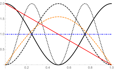
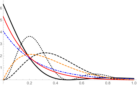
(a)	(b)
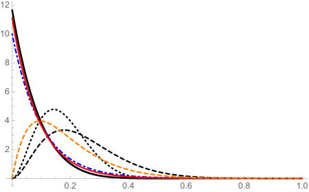
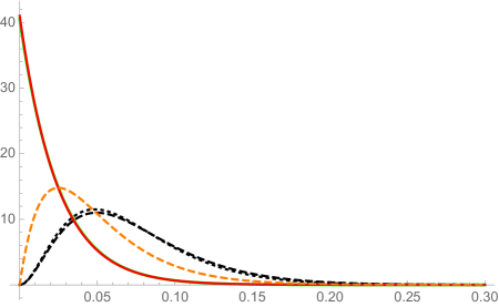
(c)	(d)

Figure 1: Sculpting of ${f_{{\cal E}{(\beta{{\cal X}_{I}})}}}(\epsilon)$ with $\beta{{{\cal X}_{I}}}$: Solid – $g_{0}(\epsilon)=1+\cos 2\pi\epsilon$; Dashed – $g_{0}(\epsilon)=1-\cos 2\pi\epsilon$; Dotted – $g_{0}(\epsilon)=1-\cos 4\pi\epsilon$; Dot-Dashed – $g_{0}(\epsilon)$ uniform; Red – $g_{0}(\epsilon)$ downsloped linear; Orange – $g_{0}(\epsilon)=\frac{\pi}{2}\sin\pi\epsilon$. Note convergence to exponential (Gamma distribution with $k=1$) for those initial distributions that are approximately constant for small $\epsilon$, Gamma with $k=2$ for the lone sinusoidal distribution that is proportional to $\epsilon$ for small $\epsilon$, and Gamma with $k=3$ for the two cosinusoidal distributions with $g_{0}(0)=0$ which are quadratic for small $\epsilon$. (a) $\beta{{{\cal X}_{I}}}=0$; (b) $\beta{{{\cal X}_{I}}}=4$; (c) $\beta{{{\cal X}_{I}}}=10$; (d) $\beta{{{\cal X}_{I}}}=40$.

It is easy to see that Gamma distributions are a sort of “eigenfunction” for susceptibility distribution evolution – an initially Gamma $g_{0}(\epsilon)$ guarantees that ${f_{{\cal E}{(t)}}}(\epsilon)$ will remain Gamma of the same order as $g_{0}(\epsilon)$ $\forall t$. This raises the possibility that the Gamma distribution is an attractor of equation (3). This is not so. However, if $g_{0}(\epsilon)$ is continuous and can be expressed as a power series (Taylor/MacLauren or fractional), then we can show that ${f_{{\cal E}{(t)}}}(\epsilon)$ will indeed approach a Gamma distribution.

First, define the compact region ${\cal R}_{\epsilon}$ with boundaries $\epsilon^{-}<\epsilon^{+}$,

$${\cal R}_{\epsilon}=\{\epsilon|\epsilon^{-}\leq\epsilon\leq\epsilon^{+}\}$$

such that

$$\int_{\epsilon^{-}}^{\epsilon^{+}}{f_{{\cal E}{(t)}}}(\epsilon)d\epsilon\approx 1$$

If $\exists{\cal R}_{\epsilon}$ such that $g_{0}(\epsilon)$ is well-approximated for $\epsilon\in{\cal R}_{\epsilon}$ by some $\theta\epsilon^{\ell}$ with $\ell>-1$ and $\theta>0$, then

$${f_{{\cal E}{(t)}}}(\epsilon)\approx C(\theta,\beta{{\cal X}_{I}})\theta\epsilon^{\ell}e^{-\beta{{\cal X}_{I}}\epsilon}$$ (19)

where $C({\theta},\beta{{\cal X}_{I}})$ is an appropriate normalization constant. Equation (19) is a Gamma distribution of order $k=\ell+1$, mean $\frac{k}{\beta{{\cal X}_{I}}}$ and variance $\frac{k}{(\beta{{\cal X}_{I}})^{2}}$. If $k$ is an integer the distribution is also Erlang (as well as Gamma), and if $k=1$ the distribution is exponential.

Then, note that equation (3) dictates the probability mass of ${f_{{\cal E}{(t)}}}(\epsilon)$ will be forced to the left with increasing time (indexed by ${{\cal X}_{I}}$) because $e^{-\beta{{\cal X}_{I}}\epsilon}$ necessarily concentrates the probability mass (and thereby the region ${\cal R}_{\epsilon}$) closer to the origin. Thus, even if $g_{0}(\epsilon)$ is arbitrary in form away from the origin, so long as ${\cal R}_{\epsilon}$ eventually covers a region where $g_{0}(\epsilon)$ approximately $\theta\epsilon^{\ell}$ for some $\ell>-1$, the density ${f_{{\cal E}{(t)}}}(\epsilon)$ will eventually be approximately a Gamma distribution with parameter $k=\ell+1$. The evolution of several different initial distributions is shown in FIGURE 1. The convergence to Gamma distributions of orders $k=1,2,3$ is as expected from small-$\epsilon$ order of the initial distributions – first order in the three cases where $g_{0}(0)\neq 0$, second order for the lone sinusoidal distribution which is linear for small $\epsilon$, and third order for the two cosinusoidal distributions with $g_{0}(0)=0$ which are quadratic for small $\epsilon$.

This argument can also be extended to cases were $\ell\leq-1$ so long as for $\epsilon^{-}>0$ we have $g_{0}(\epsilon)=0$ $\forall\epsilon<\epsilon^{-}$. To our knowledge the resultant distribution, equation (19) with $\ell\leq-1$, has no formal name. However, we note that Pareto $g_{0}(\epsilon)$ will produce ${f_{{\cal E}{(t)}}}(\epsilon)$ in this $\ell\leq 1$ class. The situation is of course more complicated if $g_{0}(\epsilon)$ cannot eventually be well-approximated by $\theta\epsilon^{\ell}$ on some limiting ${\cal R}_{\epsilon}$, is without compact support or contains singularities.

III ${\bar{\cal E}}(t)$ and the Number of Susceptibles, ${x_{S}}(t)$

Typically, ${\bar{\cal E}}$ is considered independent of population variables when evaluating the differential equations of contagion. However, when the distribution on susceptibility in a population is not singular, we will show – generalizing the development in [7] – that ${\bar{\cal E}}$ can depend strongly on the number of susceptible individuals, ${x_{S}}(t)$, according to the susceptibility distribution, ${f_{{\cal E}{(t)}}}(\epsilon)$.

For notational clarity we will drop the time variable $t$, recognizing that all quantities are functions of time under the action of contagion, including the distribution on susceptibility. Thus, if ${x_{S}}$ is the total number of susceptible individuals in a population at time $t$, we assume the number, $n_{S}(\epsilon)$, of individuals with susceptibility $\epsilon$ is

$$n_{S}(\epsilon)={x_{S}}{f_{{\cal E}}}(\epsilon)$$

We can then define $E$ as the average susceptible population (as opposed to the average susceptibility of individuals, ${\bar{\cal E}}$) as

$$E=\int_{0}^{\infty}\epsilon n_{S}(\epsilon)d\epsilon={x_{S}}{\bar{\cal E}}$$ (20)

Now, define the random variable ${{\cal E}^{\dagger}}$ as the susceptibility of those who have just fallen ill at time $t$. The distribution of ${{\cal E}^{\dagger}}$ is

$$f_{{{\cal E}^{\dagger}}}(\epsilon)=\frac{\epsilon}{{\bar{\cal E}}}{f_{{\cal E}}}(\epsilon)$$ (21)

and it has mean

$${{{\bar{\cal E}}}^{\dagger}}=\int\frac{\epsilon^{2}}{{\bar{\cal E}}}{f_{{\cal E}}}(\epsilon)d\epsilon=\frac{{{\sigma_{{\cal E}}^{2}}}}{{\bar{\cal E}}}+{\bar{\cal E}}$$ (22)

where ${{\sigma_{{\cal E}}^{2}}}$ is the variance of the susceptibility at time $t$. But we can also interpret ${{{\bar{\cal E}}}^{\dagger}}$ as the rate of change of the total susceptibility $E$ with respect to ${x_{S}}$. That is, let $\Delta\!{x_{S}}$ be the differential number of individuals removed from the susceptible pool during a time instant ${\mbox{\small$\Delta$}t\,}$. Since the newly infected’s susceptibilities follow the distribution of equation (21), the decline $\Delta\!E$ in $E$ is

$$\Delta\!E={{{\bar{\cal E}}}^{\dagger}}(t)\Delta\!{x_{S}}$$

and the ratio of $\Delta\!E$ to $\Delta\!{x_{S}}$ as ${\mbox{\small$\Delta$}t\,}\rightarrow 0$ is

$$\frac{dE}{d{x_{S}}}={{{\bar{\cal E}}}^{\dagger}}$$ (23)

Now, differentiating equation (20) with respect to ${x_{S}}$ yields

$$\frac{dE}{d{x_{S}}}={\bar{\cal E}}+{x_{S}}\frac{d{\bar{\cal E}}}{d{x_{S}}}$$

which through application of equation (23) becomes

$${{{\bar{\cal E}}}^{\dagger}}={\bar{\cal E}}+{x_{S}}\frac{d{\bar{\cal E}}}{d{x_{S}}}$$

which via equation (22) simplifies to

$$\frac{{{\sigma_{{\cal E}}^{2}}}}{{\bar{\cal E}}}={x_{S}}\frac{d{\bar{\cal E}}}{d{x_{S}}}$$ (24)

which we rearrange as

$$\frac{d{x_{S}}}{{x_{S}}}=d{\bar{\cal E}}\left({\frac{{\bar{\cal E}}}{{{\sigma_{{\cal E}}^{2}}}}}\right)$$

so that assuming ${\bar{\cal E}}(0)=1$ we have

$$\boxed{\log\left(\frac{{x_{S}}}{{x_{S}}(0)}\right)=\int_{1}^{{\bar{\cal E}}}\left(\frac{{\bar{\cal E}}}{{{\sigma_{{\cal E}}^{2}}}}\right)d{\bar{\cal E}}}$$ (25)

Equation (25) tells us that ${\bar{\cal E}}$ is explicitly a function of the contagion state variable ${x_{S}}$, a dependence which fundamentally subverts the assumption of average susceptibility as an independent parameter in the contagion dynamical equations. Rather ${\bar{\cal E}}(t)$ is a contagion state variable. Put another way, the dependence of ${\bar{\cal E}}$ on ${x_{S}}$ changes the order of the contagion differential equations, and this order may in fact be a function of time.

In the next section we explore equation (25) for several different susceptibility distribution types to motivate more formally defining an instantaneous order, ${\cal K}$, of ${\bar{\cal E}}$ with respect to ${x_{S}}$.

III-A ${x_{S}}$ vs. ${\bar{\cal E}}$ Examples

The key element of equation (25) is the expression $\frac{{\bar{\cal E}}}{{{\sigma_{{\cal E}}^{2}}}}$ and its dependence on ${\bar{\cal E}}$. For any given distribution, ${{\sigma_{{\cal E}}^{2}}}$ and ${\bar{\cal E}}$ may be independent or dependent. For instance, the mean and variance of a Gaussian distribution are independent – one can be changed without affecting the other. In contrast, the variance of an exponential distribution is the square of the mean. For many distributions, however, the mean and variance are neither as separable nor as crisply dependent, so to evaluate the integral of equation (25) we must carefully find $\frac{{\bar{\cal E}}}{{{\sigma_{{\cal E}}^{2}}}}$ as a function of ${\bar{\cal E}}$ (and other quantities independent of ${\bar{\cal E}}$).

$2$-Point ${f_{{\cal E}}}(\epsilon)$: Suppose

$${f_{{\cal E}}}(\epsilon)=p\delta(\epsilon)+(1-p)\delta\left(\epsilon-\frac{{\bar{\cal E}}}{1-p}\right)$$

with mean ${\bar{\cal E}}$ and variance $\frac{p}{1-p}{\bar{\cal E}}^{2}$. Thus

$$\frac{{\bar{\cal E}}}{{{\sigma_{{\cal E}}^{2}}}}=\frac{1-p}{p{\bar{\cal E}}}$$

Notice that selection of $p$ does not affect the mean, ${\bar{\cal E}}$, so we can safely apply equation (25) to obtain

$$\boxed{{\bar{\cal E}}=\left(\frac{{x_{S}}}{{x_{S}}(0)}\right)^{\frac{p}{1-p}}}_{\,\,\,\mbox{$2$-Point}}$$ (26)

Uniform ${f_{{\cal E}}}(\epsilon)$: Suppose ${f_{{\cal E}}}(\epsilon)$ is uniform on $[\epsilon^{-},\epsilon^{+}]$. We then have

$${\bar{\cal E}}=\frac{\epsilon^{+}-\epsilon^{-}}{2}$$

and

$${{\sigma_{{\cal E}}^{2}}}=\frac{(\epsilon^{+}-\epsilon^{-})^{2}}{12}=\frac{\left({\bar{\cal E}}\right)^{2}}{3}$$

so that

$$\frac{{\bar{\cal E}}}{{{\sigma_{{\cal E}}^{2}}}}=\frac{3}{{\bar{\cal E}}}$$

Since only ${\bar{\cal E}}$ and a constant appear we can apply equation (25) to obtain

$$\boxed{{\bar{\cal E}}=\left(\frac{{x_{S}}}{{x_{S}}(0)}\right)^{1/3}}_{\,\,\,\mbox{Uniform}}$$ (27)

Gamma-Distributed ${f_{{\cal E}}}(\epsilon)$: Suppose

$${f_{{\cal E}}}(\epsilon)=\frac{\frac{k}{{\bar{\cal E}}_{0}}}{\Gamma(k)}(\frac{k}{{\bar{\cal E}}_{0}}\epsilon)^{k-1}e^{-{\frac{k}{{\bar{\cal E}}_{0}}\epsilon}}$$

a Gamma distribution with parameter $k$ and mean ${\bar{\cal E}}_{0}$. The variance is $\frac{{\bar{\cal E}}_{0}^{2}}{k}$ so we have

$$\frac{{\bar{\cal E}}}{{{\sigma_{{\cal E}}^{2}}}}=\frac{k}{{\bar{\cal E}}}$$

which because $k$ is a fixed parameter allows us to use equation (25) to obtain

$$\boxed{{\bar{\cal E}}=\left(\frac{{x_{S}}}{{x_{S}}(0)}\right)^{1/k}}_{\,\,\,\mbox{Gamma}}$$ (28)

Note that increasing the order parameter $k$ decreases the dependence of ${\bar{\cal E}}$ on ${x_{S}}$, as we would expect since the distribution becomes more impulsive as $k$ grows.

Pareto ${f_{{\cal E}}}(\epsilon)$: Suppose ${f_{{\cal E}}}(\epsilon)$ is a Pareto distribution

$${f_{{\cal E}}}(\epsilon)=\alpha{\epsilon_{0}}^{\alpha}\epsilon^{-(1+\alpha)}$$

where $\epsilon\geq{\epsilon_{0}}>0$ and $\alpha>2$. We have

$${\bar{\cal E}}=\frac{\alpha{\epsilon_{0}}}{\alpha-1}$$

and

$${{\sigma_{{\cal E}}^{2}}}=\frac{{\epsilon_{0}}^{2}\alpha}{(\alpha-1)^{2}(\alpha-2)}=\frac{{\bar{\cal E}}^{2}}{\alpha(\alpha-2)}$$

It is certainly tempting to follow the same route as the other examples – divide ${\bar{\cal E}}$ by ${{\sigma_{{\cal E}}^{2}}}$ and integrate using equation (25). However in this case, the parameter $\alpha$ depends on ${\bar{\cal E}}$ as in

$$\alpha=\frac{{\bar{\cal E}}}{{\bar{\cal E}}-{\epsilon_{0}}}$$

So, doing the requisite substitution we have

$$\frac{{{\sigma_{{\cal E}}^{2}}}}{{\bar{\cal E}}}=\frac{({\bar{\cal E}}-{\epsilon_{0}})^{2}}{2{\epsilon_{0}}-{\bar{\cal E}}}$$

Integrating $\frac{{\bar{\cal E}}}{{{\sigma_{{\cal E}}^{2}}}}$ with respect to ${\bar{\cal E}}$ yields

$$\int_{1}^{\bar{\cal E}}\frac{2{\epsilon_{0}}-{\bar{\cal E}}}{({\bar{\cal E}}-{\epsilon_{0}})^{2}}d{\bar{\cal E}}=\frac{-{\epsilon_{0}}}{{\bar{\cal E}}-{\epsilon_{0}}}-\log({\bar{\cal E}}-{\epsilon_{0}})+\frac{{\epsilon_{0}}}{1-{\epsilon_{0}}}+\log(1-{\epsilon_{0}})$$

which reduces to

$$\boxed{\log\left(\frac{{x_{S}}}{{x_{S}}(0)}\right)=\frac{{\epsilon_{0}}({\bar{\cal E}}-1)}{({\bar{\cal E}}-{\epsilon_{0}})(1-{\epsilon_{0}})}-\log\frac{{\bar{\cal E}}-{\epsilon_{0}}}{1-{\epsilon_{0}}}}_{\,\,\,\mbox{Pareto}}$$ (29)

Expressing ${\bar{\cal E}}$ compactly in terms of ${x_{S}}$ is impossible so we are stymied in evaluating the power relationship between ${x_{S}}$ and ${\bar{\cal E}}({x_{S}})$. To establish that relationship requires new machinery.

III-B The Order Parameter ${\cal K}$

In the previous section we showed that ${\bar{\cal E}}$ can depend on ${x_{S}}$, a key state variable in the differential equations that govern contagion. Of particular note, we were able to show that if the susceptibility is initially Gamma-distributed with shape parameter $k$, then ${\bar{\cal E}}=({x_{S}}/{x_{S}}(0))^{1/k}$ and that this relationship is maintained under the action of contagion (see equation (13)). However, we know that the general action of contagion not only lowers ${\bar{\cal E}}$ over time but also changes the distribution shape as well. Thus, even if a closed form expression for order can be obtained using equation (25) with an initial susceptibility distribution $g_{0}(\epsilon)$, then with the exception of Gamma distributions, the passage of time will change the order.

For instance, starting from an initially uniform distribution with order $1/3$ as determined in equation (27), equation (6) will immediately produce a truncated exponential distribution which over time will be substantively indistinguishable from a true exponential distribution. Thus, the initial order parameter would evolve from $1/3$ in equation (27) to $1$ (corresponding to a Gamma distribution with shape parameter $k=1$).

We have already seen that ${\bar{\cal E}}$ may be a relatively complicated function of ${x_{S}}$ (equation (29)) as opposed to a simple power law (equation (28)). Furthermore, in some cases it may even be impossible to compose the integrand of equation (25) explicitly in terms of ${\bar{\cal E}}$.

We circumvent these difficulties by defining the instantaneous order, ${\cal K}$, as

$$\boxed{{{\cal K}}\equiv\frac{d(\log{\bar{\cal E}})}{d(\log{x_{S}})}}$$ (30)

That is, the variation of the $(\log{\bar{\cal E}})$ with $(\log{x_{S}})$ is explicitly a power law relationship. And while certainly the slope defined by equation (30) may change for different values of ${\bar{\cal E}}$ and ${x_{S}}$, it still defines a power law relationship between ${\bar{\cal E}}$ and ${x_{S}}$ at a given instant.

Equation (30) provides a basis for investigating the range of power laws possible between ${\bar{\cal E}}$ and ${x_{S}}$. We can derive a lower bound on ${{\cal K}}$ by noting that both $\frac{d{\bar{\cal E}}}{dt}$ and $\frac{d{x_{S}}}{dt}$ are non-positive. Thus the ratio of their differentials in equation (30) must be greater than or equal to zero so that ${\cal K}\geq 0$. We then note that via equation (18) we have ${{\cal K}=0}$ in only two circumstances – the contagion has run its course and ${\dot{{{\cal X}_{I}}}}=0$, or the variance of the susceptibility distribution is zero implying that all individuals have identical susceptibilities. For active contagion (${\dot{{{\cal X}_{I}}}}>0$) this fact is worth memorializing:

$$\boxed{\begin{array}[]{c}\mbox{If ${\dot{{{\cal X}_{I}}}}>0$, then ${\cal K}(t)\geq 0$}\\ \\ \mbox{with equality iff ${f_{{\cal E}{(t)}}}(\epsilon)$ is singular.}\end{array}}$$ (31)

To summarize, ${\bar{\cal E}}(t)$ is always a function of the contagion state variable ${x_{S}}$ unless all individuals have the same susceptibility or the contagion has run its course. Otherwise at any time $t$, ${\bar{\cal E}}(t)\propto{x_{S}^{{\cal K}(t)}}$ where ${\cal K}(t)>0$.

III-C ${\cal K}$ and ${\dot{{\cal K}}}$ in Terms of Moments

Knowing ${\cal K}$ can only be zero or positive is useful. However, explicit evaluation of equation (25) to obtain ${\cal K}$ can be difficult – witness the Pareto distribution considered previously. Nonetheless, we can always calculate ${\cal K}$ (and even its time derivative ${\dot{{\cal K}}}$) in terms of the moments of ${f_{{\cal E}{(t)}}}(\epsilon)$, either analytically or empirically.

To begin, we first write equation (25) as

$$\log\left(\frac{{x_{S}}}{{x_{S}}(0)}\right)=\int_{1}^{{\bar{\cal E}}}\frac{{\bar{\cal E}}}{{{\sigma_{{\cal E}}^{2}}}}d{\bar{\cal E}}={{\cal W}}(\log{\bar{\cal E}})$$ (32)

We then have

$$(d\log{x_{S}})=(d\log{\bar{\cal E}}){{\cal W}}^{\prime}(\log{\bar{\cal E}})$$

which via equation (30) leads to

$$\frac{1}{{\cal K}}={{\cal W}}^{\prime}(\log{\bar{\cal E}})$$ (33)

where

$${{\cal W}}^{\prime}(x)=\frac{d}{dx}{{\cal W}}(x)$$

Then, we note that if

$$F(x)=\int f(x)dx$$

we have

$$\frac{d}{dt}F(x)=\dot{x}f(x)$$

where ”dot” implies differentiation with respect to time. So, differentiating the two rightmost terms of equation (32) yields

$${{\dot{{\bar{\cal E}}}}}\frac{{\bar{\cal E}}}{{{\sigma_{{\cal E}}^{2}}}}=\frac{{{\dot{{\bar{\cal E}}}}}}{{\bar{\cal E}}}{{\cal W}}^{\prime}(\log{\bar{\cal E}})$$

so that

$${{\cal W}}^{\prime}(\log{\bar{\cal E}})=\frac{{\bar{\cal E}}^{2}}{{{\sigma_{{\cal E}}^{2}}}}$$

and

$$\boxed{{\cal K}=\frac{{{\sigma_{{\cal E}}^{2}}}}{{\bar{\cal E}}^{2}}=\frac{{\overline{{\cal E}^{2}}}}{{\bar{\cal E}}^{2}}-1}$$ (34)

where

$${\overline{{\cal E}^{2}}}=\int_{0}^{\infty}\epsilon^{2}{f_{{\cal E}{(t)}}}(\epsilon)d\epsilon$$

We note that ${\cal K}$ as defined in equation (34) is exactly the square of a quantity often called the ”coefficient-of-variation” [8].

To determine how rapidly ${\cal K}$ changes it is most convenient to differentiate equation (33) (as opposed to equation (34)) to obtain

$$\frac{d}{dt}\left(\frac{1}{{\cal K}}\right)=\frac{{{\dot{{\bar{\cal E}}}}}}{{\bar{\cal E}}}{{\cal W}}^{\prime\prime}(\log{\bar{\cal E}})=\frac{2{\bar{\cal E}}{{\dot{{\bar{\cal E}}}}}}{{{\sigma_{{\cal E}}^{2}}}}-\frac{{\bar{\cal E}}^{2}}{{{\sigma_{{\cal E}}^{2}}}^{2}}{\dot{{{\sigma_{{\cal E}}^{2}}}}}$$

Remembering that ${{\sigma_{{\cal E}}^{2}}}={\overline{{\cal E}^{2}}}-{\bar{\cal E}}^{2}$ and ${{{\dot{{\bar{\cal E}}}}}}=-\beta{{{\dot{{{\cal X}_{I}}}}}}{{{{\sigma_{{\cal E}}^{2}}}}}$ we have

$${\dot{{{\sigma_{{\cal E}}^{2}}}}}=\frac{{{\dot{{\bar{\cal E}}}}}}{{{\sigma_{{\cal E}}^{2}}}}({\overline{{\cal E}^{3}}}-{\overline{{\cal E}^{2}}}{\bar{\cal E}}-2{\bar{\cal E}}{{\sigma_{{\cal E}}^{2}}})=\frac{{{\dot{{\bar{\cal E}}}}}}{{{\sigma_{{\cal E}}^{2}}}}E\left[({\cal E}-{\bar{\cal E}})^{3}\right]$$

If we then define the distribution ”skew” as

$${{\cal S}_{{\cal E}}^{3}}\equiv\frac{E\left[({\cal E}-{\bar{\cal E}})^{3}\right]}{\sigma_{\cal E}^{3}}$$

we have

$$\frac{d}{dt}\left(\frac{1}{{\cal K}}\right)=\frac{{{\dot{{\bar{\cal E}}}}}{\bar{\cal E}}}{{{\sigma_{{\cal E}}^{2}}}}\left(2-\frac{{\bar{\cal E}}}{\sigma_{\cal E}}{{\cal S}_{{\cal E}}^{3}}\right)$$ (35)

and since $\frac{d}{dt}\left(\frac{1}{{\cal K}}\right)=-\frac{{{\dot{{\cal K}}}}}{{\cal K}^{2}}$ we obtain

$$\boxed{{{\dot{{\cal K}}}}={{\dot{{\bar{\cal E}}}}}\frac{{{\sigma_{{\cal E}}^{2}}}}{{\bar{\cal E}}^{3}}\left(\frac{{\bar{\cal E}}}{\sigma_{\cal E}}{{\cal S}_{{\cal E}}^{3}}-2\right)}$$ (36)

Applying equation (18) yields

$$\boxed{{{\dot{{\cal K}}}}=-\beta{x_{I}}\frac{\sigma_{{\cal E}}^{4}}{{\bar{\cal E}}^{3}}\left(\frac{{\bar{\cal E}}}{\sigma_{\cal E}}{{\cal S}_{{\cal E}}^{3}}-2\right)}$$ (37)

Therefore if the skew of a distribution is zero or negative, the order ${\cal K}$ under the action of contagion would initially increase. Alternatively, if there is strong positive skew so that $\frac{{\bar{\cal E}}}{\sigma_{\cal E}}{{\cal S}_{{\cal E}}^{3}}-2>0$ (as there would be for heavier-tailed distributions), then the order would initially decrease.

We can also define ${\cal K}$ (and ${\dot{{\cal K}}}$, if desired) in terms of the Laplace transform of the initial distribution $g_{0}(\epsilon)$. Defining the Laplace transform of $g_{0}(\epsilon)$ as

$$G_{0}(s)=\int_{0}^{\infty}g(\epsilon)e^{-s\epsilon}d\epsilon$$

we know that since $g_{0}(\epsilon)$ is a probability function we have

$${\bar{\cal E}}(0)=-G^{\prime}(0)$$

and

$${\overline{{\cal E}^{2}}}(0)=G_{0}^{\prime\prime}(0)$$

So, via equation (6) we have

$${\bar{\cal E}}(\beta{{\cal X}_{I}})=-\frac{G_{0}^{\prime}(\beta{{\cal X}_{I}})}{G_{0}(\beta{{\cal X}_{I}})}$$

and

$${\overline{{\cal E}^{2}}}(\beta{{\cal X}_{I}})=\frac{G_{0}^{\prime\prime}(\beta{{\cal X}_{I}})}{G_{0}(\beta{{\cal X}_{I}})}$$

so that

$$\boxed{{\cal K}(\beta{{\cal X}_{I}})=\frac{G_{0}^{\prime\prime}(\beta{{\cal X}_{I}})G_{0}(\beta{{\cal X}_{I}})}{\left(G_{0}^{\prime}(\beta{{\cal X}_{I}})\right)^{2}}-1}$$ (38)

This approach is convenient because it requires one integration to find the Laplace transform of $g_{0}(\epsilon)$ and then only differentiations thereafter.

We must emphasize that while both equation (34) and equation (36) can be used to determine snapshots of what the current order is and where it will go next, if the time courses of mean and variance can be calculated for a given initial distribution $g_{0}(\epsilon)$, then the complete time course of order ${\cal K}$ is known through equation (34). Likewise, if the Laplace transform of $g_{0}(\epsilon)$ is known, ${\cal K}$ can also be calculated through equation (38). We exercise these results in the next section.

III-D Effective Order ${\cal K}$ Examples

$2$-Point Distribution: Equation (7) via equation (6) and equation (34) yields

$$\boxed{{\cal K}_{\mbox{\tiny$2$-Point}}=\left(\frac{p}{1-p}\right)e^{\frac{\beta{{\cal X}_{I}}{\bar{\cal E}}}{1-p}}}$$ (39)

which starts at $\frac{p}{1-p}$ (agreeing with equation (26)) and increases exponentially with $\beta{{\cal X}_{I}}$.

Gamma Distribution: From equation (12), the variance of a Gamma distribution is ${\bar{\cal E}}^{2}/k$ and the skew is $2/\sqrt{k}$. Evaluation of equation (34) yields ${\cal K}=1/k$ as expected from equation (28). Likewise, evaluation of equation (36) yields identically $0$, since the order is always $1/k$ for a Gamma distribution with parameter $k$. Thus

$$\boxed{{\cal K}_{\mbox{\tiny Gamma}}=\frac{1}{k}}$$ (40)

Uniform Distribution: We have via equation (11)

$${\bar{\cal E}}_{\mbox{\tiny Uniform}}(t)=\frac{1}{\beta{{\cal X}_{I}}}\cdot\frac{1-\left(1+\beta{{\cal X}_{I}}{\epsilon_{\mbox{\tiny max}}}\right)\cdot e^{-\beta{{\cal X}_{I}}{\epsilon_{\mbox{\tiny max}}}}}{1-e^{-\beta{{\cal X}_{I}}{\epsilon_{\mbox{\tiny max}}}}}$$

and using equation (10) we calculate

$${\overline{{\cal E}^{2}}}_{\mbox{\tiny Uniform}}(t)=\frac{2-\frac{\beta{{\cal X}_{I}}{\epsilon_{\mbox{\tiny max}}}e^{-\beta{{\cal X}_{I}}{\epsilon_{\mbox{\tiny max}}}}(2+\beta{{\cal X}_{I}}{\epsilon_{\mbox{\tiny max}}})}{1-e^{-\beta{{\cal X}_{I}}{\epsilon_{\mbox{\tiny max}}}}}}{(\beta{{\cal X}_{I}})^{2}}$$

so that letting $\phi=\beta{{\cal X}_{I}}{\epsilon_{\mbox{\tiny max}}}$ we have

$$\boxed{{\cal K}_{\mbox{\tiny Uniform}}=\frac{\left(1-e^{-\phi}\right)\left(2-(2+\phi(2+\phi))e^{-\phi}\right)}{\left(1-(1+\phi)e^{-\phi}\right)^{2}}-1}$$ (41)

We can can also calculate ${\cal K}$ for the uniform distribution using equation (38). The Laplace transform of a uniform distribution on $[0,{\epsilon_{\mbox{\tiny max}}}]$ is

$$G_{0}(s)=\frac{1-e^{-s{\epsilon_{\mbox{\tiny max}}}}}{s{\epsilon_{\mbox{\tiny max}}}}$$

so that

$$-G_{0}^{\prime}(s)=\frac{1-e^{-s{\epsilon_{\mbox{\tiny max}}}}}{s^{2}{\epsilon_{\mbox{\tiny max}}}}-\frac{e^{-s{\epsilon_{\mbox{\tiny max}}}}}{s}=\frac{1-(1+s{\epsilon_{\mbox{\tiny max}}})e^{-s{\epsilon_{\mbox{\tiny max}}}}}{s^{2}{\epsilon_{\mbox{\tiny max}}}}$$

and

$$G_{0}^{\prime\prime}(s)=2\frac{1-e^{-s{\epsilon_{\mbox{\tiny max}}}}}{s^{3}{\epsilon_{\mbox{\tiny max}}}}-\frac{e^{-s{\epsilon_{\mbox{\tiny max}}}}}{s^{2}}-\frac{e^{-s{\epsilon_{\mbox{\tiny max}}}}}{s^{2}}-{\epsilon_{\mbox{\tiny max}}}\frac{e^{-s{\epsilon_{\mbox{\tiny max}}}}}{s}$$

which reduces to

$$G_{0}^{\prime\prime}(s)=\frac{2-(1+(1+s{\epsilon_{\mbox{\tiny max}}})^{2})e^{-s{\epsilon_{\mbox{\tiny max}}}}}{s^{3}{\epsilon_{\mbox{\tiny max}}}}$$

so that with $s{\epsilon_{\mbox{\tiny max}}}=\beta{{\cal X}_{I}}{\epsilon_{\mbox{\tiny max}}}=\phi$ becomes via equation (38)

$$\boxed{{\cal K}_{\mbox{\tiny Uniform (Laplace)}}=\frac{(1-e^{-\phi})(2-(1+(1+\phi)^{2})e^{-\phi})}{\left(1-(1+\phi)e^{-\phi}\right)^{2}}}$$ (42)

Equation (42) is identical to equation (41).

Pareto Distribution: Now recall that we could not derive an explicit order for the Pareto distribution. However, we know the time course of the distribution under contagion (equation (16)),

$${f_{{\cal E}{(t)}}}(\epsilon)=\frac{\alpha{\epsilon_{0}}^{\alpha}\epsilon^{-(1+\alpha)}}{\alpha E_{(1+\alpha)}(\beta{{{\cal X}_{I}}}{\epsilon_{0}})}e^{-\beta{{{\cal X}_{I}}}\epsilon}$$

and we know the time course of the mean

$${\bar{\cal E}}_{\mbox{\tiny Pareto}}(t)={\epsilon_{0}}\frac{E_{(\alpha)}({{\cal X}_{I}}\beta{\epsilon_{0}})}{E_{(1+\alpha)}({{\cal X}_{I}}\beta{\epsilon_{0}})}$$

and also ${\overline{{\cal E}^{2}}}(t)$

$${\overline{{\cal E}^{2}}}_{\mbox{\tiny Pareto}}(t)={\epsilon_{0}}^{2}\frac{E_{(\alpha-1)}({{\cal X}_{I}}\beta{\epsilon_{0}})}{E_{(1+\alpha)}({{\cal X}_{I}}\beta{\epsilon_{0}})}$$

so that

$$\boxed{{\cal K}_{\mbox{\tiny Pareto}}=\frac{E_{(\alpha+1)}({{\cal X}_{I}}\beta{\epsilon_{0}})E_{(\alpha-1)}({{\cal X}_{I}}\beta{\epsilon_{0}})}{E_{(\alpha)}^{2}({{\cal X}_{I}}\beta{\epsilon_{0}})}-1}$$ (43)

${\cal K}$

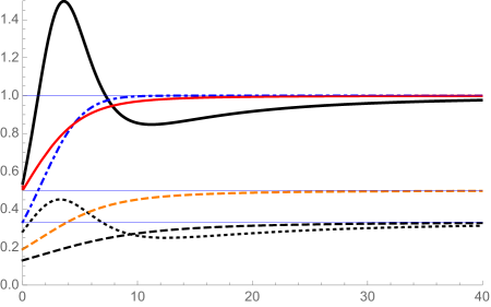
$\phi$

Figure 2: ${\cal K}$ versus $\phi=\beta{{\cal X}_{I}}$: Solid – $g_{0}(\epsilon)=1+\cos 2\pi\epsilon$; Dashed – $g_{0}(\epsilon)=1-\cos 2\pi\epsilon$; Dotted – $g_{0}(\epsilon)=1-\cos 4\pi\epsilon$; Dot-Dashed – $g_{0}(\epsilon)$ uniform; Red – $g_{0}(\epsilon)$ downsloped linear; Orange – $g_{0}(\epsilon)=\frac{\pi}{2}\sin\pi\epsilon$. Note that the asymptotes comport with the orders of the limiting $k=1,2,3$ order Gamma distributions as seen in FIGURE 1(d).

In FIGURE 2 we show the ${\cal K}$ evolution corresponding to the susceptibility distribution evolution snapshots provided in FIGURES 1. It is interesting to note that while the order asymptotes comport with the convergence to Gamma distributions of orders $k=1,2,3$ seen in FIGURE 2, the intermediate order (and thus the contagion dynamics) may vary significantly from start to finish, depending upon the initial distribution, $g_{0}(\epsilon)$.

IV The Herd Immunity Threshold

Revisiting equation (1) and equation (2), we see that the number of infections ${x_{I}}$ starts to wane when

$$\beta{\bar{\cal E}}{x_{S}}=\gamma$$

That is, since both ${\bar{\cal E}}$ and ${x_{S}}$ are strictly monotone decreasing functions of time, if $\beta{\bar{\cal E}}(0){x_{S}}(0)>\gamma$, there is a single point $t^{*}>0$ at which ${\dot{{x_{I}}}}=0$ and

$${x_{S}^{*}}={x_{S}}(t^{*})=\frac{\gamma}{\beta}\frac{1}{{\bar{\cal E}}(t^{*})}$$ (44)

$1-{{x_{S}^{*}}}$ is defined as the herd immunity threshold. It should be noted that owing to the temporal variation of ${\bar{\cal E}}(t)$, the usual final value results [9] do not directly apply. Thus, ${x_{S}^{*}}$ marks the beginning-of-the-end rather than the end of the contagion’s course.

Since we assume ${\bar{\cal E}}(0)=1$, we have ${\bar{\cal E}}(t)\leq 1$ for $t>0$, with equality iff the susceptibility distribution is singular. Thus, ${x_{S}^{*}}$ is minimized iff the susceptibility distribution is singular. We summarize this result as

$$\boxed{{x_{S}^{*}}>{x_{S}^{*}}_{\mbox{\tiny singular}}=\frac{\gamma}{\beta}}$$ (45)

That is, a singular susceptibility distribution requires the largest proportion of individuals to be infected before contagion starts to wane.

We could determine the herd immunity threshold by brute force (numerical integration of equation (1) and equation (2)). However, it is also possible to entirely avoid differential equation integration and concomitant numerical errors. As previously, we define the Laplace transform of $g_{0}(\epsilon)$ as

$$G_{0}(s)=\int_{0}^{\infty}g_{0}(\epsilon)e^{-\epsilon s}d\epsilon$$

By setting $\phi=\beta{{\cal X}_{I}}$, we can use equation (6) to write

$${\bar{\cal E}}(\phi)=\frac{-G_{0}^{\prime}(\phi)}{G_{0}(\phi)}$$ (46)

and

$${{\sigma_{{\cal E}}^{2}}}(\phi)=\frac{G_{0}(\phi)G_{0}^{\prime\prime}(\phi)-(G_{0}^{\prime}(\phi))^{2}}{G_{0}^{2}(\phi)}$$

so that

$$\frac{{\bar{\cal E}}(\phi)}{{{\sigma_{{\cal E}}^{2}}}(\phi)}=\frac{-G_{0}^{\prime}(\phi)G_{0}(\phi)}{G_{0}(\phi)G_{0}^{\prime\prime}(\phi)-(G_{0}^{\prime}(\phi))^{2}}$$

Then consider that by differentiating equation (46) we obtain

$$\frac{d{\bar{\cal E}}(\phi)}{d\phi}=-\frac{G_{0}(\phi)G_{0}^{\prime\prime}(\phi)-(G_{0}^{\prime}(\phi))^{2}}{G_{0}^{2}(\phi)}$$

so that

$$d{\bar{\cal E}}(\phi)=-\frac{G_{0}(\phi)G_{0}^{\prime\prime}(\phi)-(G_{0}^{\prime}(\phi))^{2}}{G_{0}^{2}(\phi)}d\phi$$

and the integrand $\frac{{\bar{\cal E}}(\phi)}{{{\sigma_{{\cal E}}^{2}}}(\phi)}d{\bar{\cal E}}(\phi)$ in equation (25) becomes

$$\left(\!\frac{-G_{0}^{\prime}(\phi)G_{0}(\phi)}{G_{0}(\phi)G_{0}^{\prime\prime}(\phi)\!-\!(G_{0}^{\prime}(\phi))^{2}}\!\right)\!\!\left(\!-\frac{G_{0}(\phi)G_{0}^{\prime\prime}(\phi)\!-\!(G_{0}^{\prime}(\phi))^{2}}{G_{0}^{2}(\phi)}\!\right)d\phi$$

which simplifies to

$$\frac{G_{0}^{\prime}(\phi)}{G_{0}(\phi)}d\phi$$

and allows us write

$$\log\left(\frac{{x_{S}}}{{x_{S}}(0)}\right)=\int_{0}^{\phi_{{\bar{\cal E}}}}\frac{G_{0}^{\prime}(\phi)}{G_{0}(\phi)}d\phi=\log G_{0}(\phi)\bigg{\rvert}_{0}^{\phi_{{\bar{\cal E}}}}$$ (47)

where $\phi_{{\bar{\cal E}}}$ is the value of $\phi$ for which equation (46) evaluates to ${\bar{\cal E}}$. Since $G_{0}(0)=1$, equation (47) reduces to

$${x_{S}}({\bar{\cal E}}(\phi_{{\bar{\cal E}}}))=G_{0}(\phi_{{\bar{\cal E}}}){x_{S}}(0)$$ (48)

Then, since ${x_{S}}(\cdot)$ is effectively parametrized in $\phi$, we can rewrite equation (48) as

$${x_{S}}(\phi)=G_{0}(\phi){x_{S}}(0)$$

and use equation (46) to obtain ${\bar{\cal E}}(\phi)$ so that we have

$${\bar{\cal E}}(\phi){x_{S}}(\phi)=\frac{-G_{0}^{\prime}(\phi)}{G_{0}(\phi)}G_{0}(\phi){x_{S}}(0)=-G_{0}^{\prime}(\phi){x_{S}}(0)$$

We can then identify the value $\phi^{*}$ for which equation (44) is satisfied via

$$\boxed{-G_{0}^{\prime}(\phi^{*}){x_{S}}(0)=\frac{\gamma}{\beta}}$$ (49)

to obtain the herd immunity threshold as

$$\boxed{1-{x_{S}^{*}}=1-G_{0}(\phi^{*}){x_{S}}(0)}$$ (50)

We can now exercise equation (49) and equation (50) for different $g_{0}(\epsilon)$. However, since $-G_{0}^{\prime}(\phi)$ is strictly monotone decreasing we must always assume

$$-G_{0}^{\prime}(0){x_{S}}(0)={\bar{\cal E}}(0){x_{S}}(0)\geq\frac{\gamma}{\beta}$$ (51)

Otherwise the solution $\phi^{*}$ to equation (49) does not exist. Put another way, if equation (51) is violated, contagion fizzles out.

Singular Distribution: We have

$$G_{0}(\phi)=e^{-\phi}$$

and

$$-G_{0}^{\prime}(\phi)=e^{-\phi}$$

so that

$$\phi^{*}=-\log\frac{\gamma}{\beta{x_{S}}(0)}$$

and

$$\boxed{{x_{S}^{*}}=\frac{\gamma}{\beta}}_{\,\,\,\mbox{\footnotesize herd singular}}$$ (52)

which yields ${x_{S}^{*}}=0.5$ if $\frac{\gamma}{\beta}=\frac{1}{2}$.

$2$-Point Distribution: We have

$$G_{0}(\phi)=p+(1-p)e^{-\frac{1}{1-p}\phi}$$

so that

$$-G_{0}^{\prime}(\phi)=e^{-\frac{1}{1-p}\phi}$$

We then have

$$\phi^{*}=-(1-p)\log\frac{\gamma}{\beta{x_{S}}(0)}$$

so that

$$\boxed{{x_{S}^{*}}=p{x_{S}}(0)+(1-p)\frac{\gamma}{\beta}}_{\,\,\,\mbox{\footnotesize herd 2-Point}}$$ (53)

with the proviso that ${x_{S}}(0)\geq\frac{\gamma}{\beta}$ so that ${x_{S}}(0)-{x_{S}^{*}}\geq 0$. This restriction comports with the fact that the worst herd immunity threshold is $\frac{\gamma}{\beta}$ as given in equation (52). If $\frac{\gamma}{\beta}=\frac{1}{2}$ and ${x_{S}}(0)=1$ we then have

$${x_{S}^{*}}=\frac{1}{2}(1+p)$$

Uniform Distribution: We have

$$G_{0}(\phi)=\frac{1-e^{-2\phi}}{2\phi}$$

and

$$-G_{0}^{\prime}(\phi)=\frac{1-e^{-2\phi}}{2\phi^{2}}-\frac{2e^{-2\phi}}{2\phi}$$

If $\frac{\gamma}{\beta}=\frac{1}{2}$ and ${x_{S}}(0)=1$, we numerically find

$$\phi^{*}=0.546$$

and thence

$${x_{S}^{*}}=0.609$$

Gamma Distribution: We have

$$g_{0}(\epsilon)=\frac{k}{\Gamma(k)}(k\epsilon)^{k-1}e^{-k\epsilon}$$

and

$$G_{0}(\phi)=\left(\frac{1}{\frac{\phi}{k}+1}\right)^{k}$$

so that

$$G_{0}^{\prime}(\phi)=-\left(\frac{1}{\frac{\phi}{k}+1}\right)^{k+1}$$

so that

$$\phi^{*}=k\left(\left(\frac{\gamma}{\beta}\right)^{-\frac{1}{k+1}}-1\right)$$

and

$$\boxed{{x_{S}^{*}}=\left({x_{S}}(0)\right)^{\frac{1}{k+1}}\left(\frac{\gamma}{\beta}\right)^{\frac{k}{k+1}}}_{\,\,\,\mbox{\footnotesize herd Gamma}}$$ (54)

Then, for $\frac{\gamma}{\beta}=\frac{1}{2}$, ${x_{S}}(0)=1$ and

$$k=\{0.5,1.0,2.0\}$$

we have

$${x_{S}^{*}}=\{0.794,0.707,0.630\}$$

Pareto Distribution: We have

$$\epsilon_{0}\frac{\alpha}{\alpha-1}=1$$

so that

$$\epsilon_{0}=\frac{\alpha-1}{\alpha}$$

and thence

$$g_{0}(\epsilon)=\alpha\left(\frac{\alpha-1}{\alpha}\right)^{\alpha}\epsilon^{-(\alpha+1)}$$

so that

$$G_{0}(\phi)=\alpha E_{1+\alpha}\left(\frac{\alpha-1}{\alpha}\phi\right)$$

and

$$-G_{0}^{\prime}(\phi)=(\alpha-1)E_{\alpha}\left(\frac{\alpha-1}{\alpha}\phi\right)$$

If $\frac{\gamma}{\beta}=\frac{1}{2}$, ${x_{S}}(0)=1$ and

$$\alpha=\{1.1,1.5,2.0,3.0\}$$

we have

$$\phi^{*}=\{0.00554,0.367,0.535,0.629\}$$

and

$${x_{S}^{*}}=\{0.997,0.886,0.887,0.828\}$$

V Discussion

We have shown that the shape of the population susceptibility distribution can significantly affect the time course of contagion and its ultimate severity. Since contagion modeling must ultimately be in the service of contagion understanding and control, two issues immediately come to mind:

• Given an initial population susceptibility density $g_{0}(\epsilon)$, might there be good targeted intervention strategies for contagion control?

• If population susceptibility is indeed variable, how might we efficiently and rapidly measure ${f_{{\cal E}{(t)}}}(\epsilon)$?

We discuss these issues in the next two subsections.

V-A Intervention

Suppose we are allowed to intervene and change some fraction of population susceptibilities. What reassignment maximizes the resulting herd immunity threshold? The intuitively obvious answer is to inoculate that fraction of individuals, effectively setting their susceptibilities to zero. Likewise, if the particular fraction of the population can be chosen it seems equally obvious that we should choose those individuals with greatest susceptibility.

It should be noted, however, that implementing the susceptibility zeroing abstraction faithfully may be difficult depending upon the practical methods available to mute susceptibility. For instance, perfect protection (through inoculation, isolation, and/or behavior modification) of individuals serving critical high-exposure societal functions may be impossible. Furthermore, even if those individuals who take ill are effectively removed from the equation, others must take their place, which may result in no change to the population susceptibility distribution. Nonetheless, assuming we could sculpt the population susceptibility distribution through intervention, it is still useful to show analytically that zeroing individual susceptibilities produces the best herd immunity threshold, and that the absolute best herd immunity threshold is achieved by inoculating that fraction of individuals with the highest susceptibilities.

To begin, let $g_{0}(\epsilon)$, the initial susceptibility distribution, be the weighted sum of two arbitrary singularity-free distributions $g_{1}(\epsilon)$ and $g_{2}(\epsilon)$:

$$g_{0}(\epsilon)=(1-p)g_{1}(\epsilon)+pg_{2}(\epsilon)$$ (55)

where $0<p<1$.

${x_{S}^{*}}$ is obtained through equation (50) as

$$\frac{{x_{S}^{*}}}{{x_{S}}(0)}=G_{0}(\phi^{*})=(1-p)G_{1}(\phi^{*})+pG_{2}(\phi^{*})$$ (56)

where $\phi^{*}$ satisfies equation (49):

$$G_{0}^{\prime}(\phi^{*})=\left((1-p)G_{1}^{\prime}(\phi^{*})+pG_{2}^{\prime}(\phi^{*})\right)=-\frac{\gamma}{{x_{S}}(0)\beta}$$ (57)

We then seek a replacement for $g_{2}(\epsilon)$ that maximizes ${x_{S}^{*}}$.

Since $-G_{1}^{\prime}(\phi)$ is monotonically decreasing in $\phi$ we can minimize $\phi^{*}$ in equation (57) by setting $G_{2}^{\prime}(\phi)=0$ which implies $g_{2}(\epsilon)=\delta(\epsilon)$. Since $G_{1}(\phi)$ is also monotonically decreasing in $\phi$, minimizing $\phi^{*}$ maximizes $G_{1}(\phi^{*})$. Then we note that setting $g_{2}(\epsilon)=\delta(\epsilon)$ also produces maximum $G_{2}(\phi)=1$ $\forall\phi$. Therefore, taking the probability mass $p$ associated with $pg_{2}(\epsilon)$ and relocating it to $\epsilon=0$ maximizes equation (56).

Having established that we should inoculate the population fraction represented by $pg_{2}(\epsilon)$, we can now consider how $g_{1}(\epsilon)$ should be chosen to absolutely maximize ${x_{S}^{*}}$ under the constraint of equation (55). Since it is always best to set $g_{2}(\epsilon)=\delta(\epsilon)$, we rewrite equation (56) with $G_{2}(\phi)=1$ as

$$\frac{{x_{S}^{*}}}{{x_{S}}(0)}=(1-p)G_{1}(\phi^{*})+p$$ (58)

Then we consider that since

$$G_{1}(\phi)=\int g_{1}(\epsilon)e^{-\epsilon\phi}d\epsilon$$

and $e^{-\epsilon\phi}$ is strictly monotone decreasing in $\epsilon$, we can maximize $G_{1}(\phi)$ $\forall\phi>0$ (and thereby equation (58)) by placing as much probability mass as possible “ on the left” in $\epsilon\in[0,\epsilon^{*}]$ with $\epsilon^{*}$ chosen to satisfy

$$\int_{0}^{\epsilon^{*}}g_{0}(\epsilon)d\epsilon=1-p$$ (59)

Equation (55) requires $(1-p)g_{1}(\epsilon)\leq g_{0}(\epsilon)$ since probability densities cannot be negative. Thus, setting $g_{1}(\epsilon)=g_{0}(\epsilon)/(1-p)$ on $[0<\epsilon\leq\epsilon^{*}]$ and zero elsewhere moves the maximum allowable amount of probability mass to the left and thereby uniquely maximizes $G_{1}(\phi)$ $\forall\phi$. Applying this result to the definition of $g_{0}(\epsilon)$ in equation (55) leads to,

$$\begin{array}[]{c}g_{1}(\epsilon)=\left\{\begin{array}[]{ll}\displaystyle{g_{0}(\epsilon)}&{\epsilon\leq\epsilon^{*}}\\ \displaystyle{0}&{\mbox{o.w.}}\end{array}\right.\\ g_{2}(\epsilon)=\left\{\begin{array}[]{ll}\displaystyle{g_{0}(\epsilon)}&{\epsilon>\epsilon^{*}}\\ \displaystyle{0}&{\mbox{o.w.}}\end{array}\right.\end{array}$$ (60)

That is, $g_{1}(\epsilon)=g_{0}(\epsilon)$ for $\epsilon\in[0,\epsilon^{*}]$ and zero elsewhere is the “head” of $g_{0}(\epsilon)$ and $g_{2}(\epsilon)=g_{0}(\epsilon)$ for $\epsilon\in(\epsilon^{*},\infty)$ and zero elsewhere is the “tail” of $g_{0}(\epsilon)$.

We note that if $g_{0}(\epsilon)$ contain singularities, then it may be impossible to satisfy equation (59) as written. However, the same driving principle holds – placing as much probability mass as possible to the left in $g_{1}(\epsilon)$. We would thus relax the strict inequality in equation (60) to allow some fraction of the singular mass at $\epsilon^{*}$ to remain in the tail $g_{2}(\epsilon)$ such that $(1-p)g_{1}(\epsilon^{*})+pg_{2}(\epsilon^{*})=g_{0}(\epsilon^{*})$ while still satisfying equation (59).

So, as expected, if we can intervene during the progression of contagion and reassign some fraction $p$ of susceptibilities, we should choose those individuals with greatest susceptibility and inoculate them. The result also suggests a simple inoculation strategy if we wish to immediately quell contagion: inoculate a fraction $p$ sufficient to drive ${\bar{\cal E}}=\frac{\gamma}{\beta}$. Assuming ${\bar{\cal E}}(0)=1$ and $\frac{\gamma}{\beta}=\frac{1}{2}$ this means we must inoculate $50\%$ of the population if everyone has the same susceptibility, $\approx\!\!\!30\%$ if the initial susceptibility distribution is uniform and $\approx\!\!19\%$ if the initial susceptibility distribution is exponential.

V-B Susceptibility Variation Measurement

The notion of contagion intervention and control based on population susceptibility distribution begs the question of how susceptibility [4] can be measured. There are perhaps immunological assays that could be applied to a population which could determine the likelihood that a given individual would succumb to the illness after exposure to some unit dose. Given the difficulty and expense associated with timely testing for infection, such an approach may be unwieldy. Furthermore, if it is likely that individuals drawn from an immunologically naive population have near identical innate dose/response reactions to a particular contagion, then not only would such pre-infectious medical monitoring be costly, it would also be useless since differentially applied interventions based on susceptibility would have no effect on contagion progression.

However, if the specific contagion can only be transmitted through proximate contact (as opposed to truly airborne over large distances), then two obvious measures of susceptibility come to mind:

• protective behaviors (e.g., mask-wearing and hygiene)

• number of contacts [10, 5]

Poor hygiene, lack of protection and high numbers of contacts all potentially result in higher cumulative contagion dose and thus a higher probability of becoming infected. While hygiene monitoring seems difficult (if not invasive), surveillance and telecommunications infrastructure, suitably anonymized, might allow some measure of susceptibility variation to be obtained. Mask-wearing volume could be measured and close contact recorded through cell phone records. Of particular interest, neither of these methods would rely on medical testing a priori so that these proxies for susceptibility would lead as opposed to lag contagion and permit more effective targeted contagion control.

Of course, whether contact intensity and observable behavior are reasonable proxies for susceptibility is debatable. Nonetheless, it seems worthwhile to examine whether it is possible to cobble together at least a rough susceptibility profile estimate for a population that could inform public health interventions – again, ahead of as opposed to lagging contagion as all medically-based detection necessarily does.

VI Conclusion

We have mathematically refined the insights first introduced in [7] to show how population susceptibility variation under an assumption of static individual susceptibility affects the dynamics of contagion progression. Specifically, by positing that susceptibility might vary over a population, we defined the population susceptibility probability density ${f_{{\cal E}{(t)}}}(t)$, the time-varying average susceptibility ${\bar{\cal E}}(t)$ and developed closed-form expressions to show how these modifications to the usual SIR differential equations affect the dynamics of contagion and at what population fraction we can expect herd immunity to begin muting it. We showed that a population with singular susceptibility (everyone has the same static susceptibility) has the worst herd immunity threshold and the worst response to intervention in terms of what fraction of individuals must be inoculated to initiate herd immunity. We also showed that for a variety of possible population susceptibility distribution assumptions that the herd immunity threshold could be much lower and concomitantly, the effects of intervention more potent.

We then discussed population susceptibility measurement through the proxies of individual mobility and contact intensity as well as individual protective behaviors (such as mask-wearing). If these are indeed reasonable and lag-less proxies for susceptibility, the use of non-medical electronic susceptibility monitoring and the closed-form contagion state expressions derived here seems an interesting line of research in the prediction and control of contagion. Combined with recent hypotheses suggesting population susceptibility variation changes the progression and ultimate severity of SARS-CoV-2 [8, 11, 12], we feel that real-time measurement of susceptibility could be a critically important determinant of policy to control future pandemics.

References

[1]
Fred Brauer and Carlos Castillo-Chavez.
Mathematical Models in Population Biology and Epidemiology.
Springer New York, 2012.
[2]
Alexandru Dan Corlan and John Ross.
Kinetics methods for clinical epidemiology problems.
Proceedings of the National Academy of Sciences,
112(46):14150–14155, 2015.
[3]
Greg Dwyer, Joseph S. Elkinton, and John P. Buonaccorsi.
Host heterogeneity in susceptibility and disease dynamics: Tests of a
mathematical model.
Am. Nat., 150(6):685–707, December 1997.
[4]
Dominic Kwiatkowski.
Susceptibility to infection.
BMJ, 321(7268):1061–1065, 2000.
[5]
J. O. Lloyd-Smith, S. J. Schreiber, P. E. Kopp, and W. M. Getz.
Superspreading and the effect of individual variation on disease
emergence.
Nature, 438(7066):355–359, November 2005.
[6]
G.F. Simmons.
Differential Equations with Applications and Historical
Notes.
McGraw-Hill Book Company, New York, NY, 1972.
[7]
Christopher Rose, Andrew J. Medford, C. Franklin Goldsmith, Tejs Vegge,
Joshua S. Weitz, and Andrew A. Peterson.
Heterogeneity in susceptibility dictates the order of epidemiological
models.
arXiv, 2020.
arXiv:2005.04704v2 [q-bio.PE].
[8]
M. Gabriela M. Gomes, Rodrigo M. Corder, Jessica G. King, Kate E. Langwig,
Caetano Souto-Maior, Jorge Carneiro, Guilherme Goncalves, Carlos
Penha-Goncalves, Marcelo U. Ferreira, and Ricardo Aguas.
Individual variation in susceptibility or exposure to sars-cov-2
lowers the herd immunity threshold.
medRxiv, 2020.
2020.04.27.20081893.
[9]
Junling Ma and David J. D. Earn.
Generality of the final size formula for an epidemic of a newly
invading infectious disease.
Bull. Math. Biol., 68(3):679–702, April 2006.
[10]
Duygu Balcan, Vittoria Colizza, Bruno Gonçalves, Hao Hu, José J.
Ramasco, and Alessandro Vespignani.
Multiscale mobility networks and the spatial spreading of infectious
diseases.
Proceedings of the National Academy of Sciences,
106(51):21484–21489, 2009.
[11]
Tom Britton, Frank Ball, and Pieter Trapman.
A mathematical model reveals the influence of population
heterogeneity on herd immunity to sars-cov-2.
Science, 369(6505):846–849, August 2020.
DOI:10.1126/science.abc6810.
[12]
Laurent Hébert-Dufresne, Benjamin M. Althouse, Samuel V. Scarpino, and Antoine
Allard.
Beyond : Heterogeneity in secondary infections and
probabilistic epidemic forecasting.
ArXiV, 2020.
2002.04004.