Resource-Aware Discretization of Accelerated Optimization Flows

Abstract

This paper tackles the problem of discretizing accelerated optimization flows while retaining their convergence properties. Inspired by the success of resource-aware control in developing efficient closed-loop feedback implementations on digital systems, we view the last sampled state of the system as the resource to be aware of. The resulting variable-stepsize discrete-time algorithms retain by design the desired decrease of the Lyapunov certificate of their continuous-time counterparts. Our algorithm design employs various concepts and techniques from resource-aware control that, in the present context, have interesting parallelisms with the discrete-time implementation of optimization algorithms. These include derivative- and performance-based triggers to monitor the evolution of the Lyapunov function as a way of determining the algorithm stepsize, exploiting sampled information to enhance algorithm performance, and employing high-order holds using more accurate integrators of the original dynamics. Throughout the paper, we illustrate our approach on a newly introduced continuous-time dynamics termed heavy-ball dynamics with displaced gradient, but the ideas proposed here have broad applicability to other globally asymptotically stable flows endowed with a Lyapunov certificate.

I Introduction

A recent body of research seeks to understand the acceleration phenomena of first-order discrete optimization methods by means of models that evolve in continuous time. Roughly speaking, the idea is to study the behavior of ordinary differential equations (ODEs) which arise as continuous limits of discrete-time accelerated algorithms. The basic premise is that the availability of the powerful tools of the continuous realm, such as differential calculus, Lie derivatives, and Lyapunov stability theory, can be then brought to bear to analyze and explain the accelerated behavior of these flows, providing insight into their discrete counterparts. Fully closing the circle to provide a complete description of the acceleration phenomenon requires solving the outstanding open question of how to discretize the continuous flows while retaining their accelerated convergence properties. However, the discretization of accelerated flows has proven to be a challenging task, where retaining acceleration seems to depend largely on the particular ODE and the discretization method employed. This paper develops a resource-aware approach to the discretization of accelerated optimization flows.

Literature Review

The acceleration phenomenon goes back to the seminal paper [1] introducing the so-called heavy-ball method, which employed momentum terms to speed up the convergence of the classical gradient descent method. The heavy-ball method achieves optimal convergence rate in a neighborhood of the minimizer for arbitrary convex functions and global optimal convergence rate for quadratic objective functions. Later on, the work [2] proposed the Nesterov’s accelerated gradient method and, employing the technique of estimating sequences, showed that it converges globally with optimal convergence rate for convex and strongly-convex smooth functions. The algebraic nature of the technique of estimating sequences does not fully explain the mechanisms behind the acceleration phenomenon, and this has motivated many approaches in the literature to provide fundamental understanding and insights. These include coupling dynamics [3], dissipativity theory [4], integral quadratic constraints [5, 6], and geometric arguments [7].

Of specific relevance to this paper is a recent line of research initiated by [8] that seeks to understand the acceleration phenomenon in first-order optimization methods by means of models that evolve in continuous time. [8] introduced a second-order ODE as the continuous limit of Nesterov’s accelerated gradient method and characterized its accelerated convergence properties using Lyapunov stability analysis. The ODE approach to acceleration now includes the use of Hamiltonian dynamical systems [9, 10], inertial systems with Hessian-driven damping [11], and high-resolution ODEs [12, 13]. This body of research is also reminiscient of the classical dynamical systems approach to algorithms in optimization, see [14, 15]. The question of how to discretize the continuous flows while maintaining their accelerated convergence rates has also attracted significant attention, motivated by the ultimate goal of fully understanding the acceleration phenomenon and taking advantage of it to design better optimization algorithms. Interestingly, discretizations of these ODEs do not necessarily lead to acceleration [16]. In fact, explicit discretization schemes, like forward Euler, can even become numerically unstable after a few iterations [17]. Most of the discretization approaches found in the literature are based on the study of well-known integrators, including symplectic integrators [9, 18], Runge-Kutta integrators [19] or modifications of Nesterov’s three sequences [17, 18, 20]. Our previous work [21] instead developed a variable-stepsize discretization using zero-order holds and state-triggers based on the derivative of the Lyapunov function of the original continuous flow. Here, we provide a comprehensive approach based on powerful tools from resource-aware control, including performance-based triggering and state holds that more effectively use sampled information. Other recent approaches to the acceleration phenomena and the synthesis of optimization algorithms using control-theoretic notions and techniques include [22], which employs hybrid systems to design a continuous-time dynamics with a feedback regulator of the viscosity of the heavy-ball ODE to guarantee arbitrarily fast exponential convergence, and [23], which introduced an algorithm which alternates between two (one fast when far from the minimizer but unstable, and another slower but stable around the minimizer) continuous heavy-ball dynamics.

Statement of Contributions

This paper develops a resource-aware control framework to the discretization of accelerated optimization flows that fully exploits their dynamical properties. Our approach relies on the key observation that resource-aware control provides a principled way to go from continuous-time control design to real-time implementation with stability and performance guarantees by opportunistically prescribing when certain resource should be employed. In our treatment, the resource to be aware of is the last sampled state of the system, and hence what we seek to maximize is the stepsize of the resulting discrete-time algorithm. Our first contribution is the introduction of a second-order differential equation which we term heavy-ball dynamics with displaced gradient. This dynamics generalizes the continuous-time heavy-ball dynamics analyzed in the literature by evaluating the gradient of the objective function taking into account the second-order nature of the flow. We establish that the proposed dynamics retains the same convergence properties as the original one while providing additional flexibility in the form of a design parameter.

Our second contribution uses trigger design concepts from resource-aware control to synthesize criteria that determine the variable stepsize of the discrete-time implementation of the heavy-ball dynamics with displaced gradient. We refer to these criteria as event- or self-triggered, depending on whether the stepsize is implicitly or explicitly defined. We employ derivative- and performance-based triggering to ensure the algorithm retains the desired decrease of the Lyapunov function of the continuous flow. In doing so, we face the challenge that the evaluation of this function requires knowledge of the unknown optimizer of the objective function. To circumvect this hurdle, we derive bounds on the evolution of the Lyapunov function that can be evaluated without knowledge of the optimizer. We characterize the convergence properties of the resulting discrete-time algorithms, establishing the existence of a minimum inter-event time and performance guarantees with regards to the objective function.

Our last two contributions provide ways of exploiting the sampled information to enhance the algorithm performance. Our third contribution provides an adaptive implementation of the algorithms that adaptively adjusts the value of the gradient displacement parameter depending on the region of the space to which the state belongs. Our fourth and last contribution builds on the fact that the continuous-time heavy-ball dynamics can be decomposed as the sum of a second-order linear dynamics with a nonlinear forcing term corresponding to the gradient of the objective function. Building on this observation, we provide a more accurate hold for the resource-aware implementation by using the samples only on the nonlinear term, and integrating exactly the resulting linear system with constant forcing. We establish the existence of a minimum inter-event time and characterize the performance with regards to the objective function of the resulting high-order-hold algorithm. Finally, we illustrate the proposed optimization algorithms in simulation, comparing them against the heavy-ball and Nesterov’s accelerated gradient methods and showing superior performance to other discretization methods proposed in the literature.

II Preliminaries

This section presents basic notation and preliminaries.

II-A Notation

We denote by ${\mathbb{R}}$ and $\mathbb{R}_{>0}$ the sets of real and positive real numbers, resp. All vectors are column vectors. We denote their scalar product by $\langle\cdot,\cdot\rangle$. We use $\left\lVert\cdot{}\right\rVert$ to denote the $2$-norm in Euclidean space. Given $\mu\in\mathbb{R}_{>0}$, a continuously differentiable function $f$ is $\mu$-strongly convex if $f(y)-f(x)\geq\langle\nabla f(x),y-x\rangle+\frac{\mu}{2}\left\lVert x-y\right\rVert^{2}$ for $x$, $y\in{\mathbb{R}}^{n}$. Given $L\in\mathbb{R}_{>0}$ and a function $f:X\rightarrow Y$ between two normed spaces $(X,\left\lVert\cdot{}\right\rVert_{X})$ and ($Y,\left\lVert\cdot{}\right\rVert_{Y}$), $f$ is $L$-Lipschitz if $\left\lVert f(x)-f(x^{\prime})\right\rVert_{Y}\leq L\left\lVert x-x^{\prime}\right\rVert_{X}$ for $x$, $x^{\prime}\in X$. The functions we consider here are continuously differentiable, $\mu$-strongly convex and have $L$-Lipschitz continuous gradient. We refer to the set of functions with all these properties by $\mathcal{S}_{\mu,L}^{1}({\mathbb{R}}^{n})$. A function $f:{\mathbb{R}}^{n}\rightarrow{\mathbb{R}}$ is positive definite relative to $x_{*}$ if $f(x_{*})=0$ and $f(x)>0$ for $x\in{\mathbb{R}}^{n}\setminus\{x_{*}\}$.

II-B Resource-Aware Control

Our work builds on ideas from resource-aware control to develop discretizations of continuous-time accelerated flows. Here, we provide a brief exposition of its basic elements and refer to [24, 25] for further details.

Given a controlled dynamical system $\dot{p}=X(p,u)$, with $p\in{\mathbb{R}}^{n}$ and $u\in{\mathbb{R}}^{m}$, assume we are given a stabilizing continuous state-feedback $\mathfrak{k}:{\mathbb{R}}^{n}\rightarrow{\mathbb{R}}^{m}$ so that the closed-loop system $\dot{p}=X(p,\mathfrak{k}(p))$ has $p_{*}$ as a globally asymptotically stable equilibrium point. Assume also that a Lyapunov function $V:{\mathbb{R}}^{n}\rightarrow{\mathbb{R}}$ is available as a certificate of the globally stabilizing nature of the controller. Here, we assume this takes the form

$$\dot{V}=\langle\nabla V(p)X(p,\mathfrak{k}(p))\rangle\leq-\frac{\sqrt{\mu}}{4}V(p),$$ (1)

for all $p\in{\mathbb{R}}^{n}$. Although exponential decay of $V$ along the system trajectories is not necessary, we restrict our attention to this case as it arises naturally in our treatment.

Suppose we are given the task of implementing the controller signal over a digital platform, meaning that the actuator cannot be continuously updated as prescribed by the specification $u=\mathfrak{k}(p)$. In such case, one is forced to discretize the control action along the execution of the dynamics, while making sure that stability is still preserved. A simple-to-implement approach is to update the control action periodically, i.e., fix $h>0$, sample the state as $\{p(kh)\}_{k=0}^{\infty}$ and implement

$$\dot{p}(t)=X(p(t),\mathfrak{k}(p(kh))),\quad t\in[kh,(k+1)h].$$

This approach requires $h$ to be small enough to ensure that $V$ remains a Lyapunov function and, consequently, the system remains stable. By contrast, in resource-aware control, one employs the information generated by the system along its trajectory to update the control action in an opportunistic fashion. Specifically, we seek to determine in a state-dependent fashion a sequence of times $\{t_{k}\}_{k=0}^{\infty}$, not necessarily uniformly spaced, such that $p_{*}$ remains a globally asymptotically stable equilibrium for the system

$$\dot{p}(t) =X(p(t),\mathfrak{k}(p(t_{k}))),\quad t\in[t_{k},t_{k+1}].$$ (2)

The main idea to accomplish this is to let the state sampling be guided by the principle of maintaining the same type of exponential decay (1) along the new dynamics. To do this, one defines triggers to ensure that this decay is never violated by prescribing a new state sampling. Formally, one sets $t_{0}=0$ and $t_{k+1}=t_{k}+\operatorname{step}(p(t_{k}))$, where the stepsize is defined by

$$\operatorname{step}(\hat{p}) =\min\{t>0\;|\;b(\hat{p},t)=0\}.$$ (3)

We refer to the criteria as event-triggering or self-triggering depending on whether the evaluation of the function $b$ requires monitoring of the state $p$ along the trajectory of (2) (ET) or just knowledge of its initial condition $\hat{p}$ (ST). The more stringent requirements to implement event-triggering lead to larger stepsizes versus the more conservative ones characteristic of self-triggering. In order for the state sampling to be implementable in practice, the inter-event times $\{t_{k+1}-t_{k}\}_{k=0}^{\infty}$ must be uniformly lower bounded by a positive minimum inter-event time, abbreviated MIET. In particular, the existence of a MIET rules out the existence of Zeno behavior, i.e., the possibility of an infinite number of triggers in a finite amount of time.

Depending on how the evolution of the function $V$ is examined, we describe two types of triggering conditions:

In this case, $b^{\operatorname{d}}$ is defined as an upper bound of the expression $\frac{d}{dt}V(p(t;\hat{p}))+\frac{\sqrt{\mu}}{4}V(p(t;\hat{p}))$. This definition ensures that (1) is maintained along (2);

In this case, $b^{\operatorname{p}}$ is defined as an upper bound of the expression $V(p(t;\hat{p}))-e^{-\frac{\sqrt{\mu}}{4}t}V(\hat{p})$. Note that this definition ensures that the integral version of (1) is maintained along (2). In general, the performance-based trigger gives rise to stepsizes that are at least as large as the ones determined by the derivative-based approach, cf. [26]. This is because the latter prescribes an update as soon as the exponential decay is about to be violated, and therefore, does not take into account the fact that the Lyapunov function might have been decreasing at a faster rate since the last update. Instead, the performance-based approach reasons over the accumulated decay of the Lyapunov function since the last update, potentially yielding longer inter-sampling times.

A final point worth mentioning is that, in the event-triggered control literature, the notion of resource to be aware of can be many different things, beyond the actuator described above, including the sensor, sensor-controller communication, communication with other agents, etc. This richness opens the way to explore more elaborate uses of the sampled information beyond the zero-order hold in (2), something that we also leverage later in our presentation.

III Problem Statement

Our motivation here is to show that principled approaches to discretization can retain the accelerated convergence properties of continuous-time dynamics, fill the gap between the continuous and discrete viewpoints on optimization algorithms, and lead to the construction of new ones. Throughout the paper, we focus on the continuous-time version of the celebrated heavy-ball method [1]. Let $f$ be a function in $\mathcal{S}_{\mu,L}^{1}({\mathbb{R}}^{n})$ and let $x_{*}$ be its unique minimizer. The heavy-ball method is known to have an optimal convergence rate in a neighborhood of the minimizer. For its continuous-time counterpart, consider the following $s$-dependent family of second-order differential equations, with $s\in\mathbb{R}_{>0}$, proposed in [12],

$$\begin{bmatrix}\dot{x}\\ \dot{v}\end{bmatrix} =\begin{bmatrix}v\\ -2\sqrt{\mu}v-(1+\sqrt{\mu s})\nabla f(x))\end{bmatrix},$$ (4a)

$$x(0) =x_{0},\quad v(0)=-\frac{2\sqrt{s}\nabla f(x_{0})}{1+\sqrt{\mu s}}.$$ (4b)

We refer to this dynamics as $X_{\operatorname{hb}}$. The following result characterizes the convergence properties of (4) to $p_{*}=[x_{*},0]^{T}$.

Theorem III.1 ([12]).

Let $V:{\mathbb{R}}^{n}\times{\mathbb{R}}^{n}\rightarrow{\mathbb{R}}$ be

$$V(x,v) =(1+\sqrt{\mu s})(f(x)-f(x_{*}))+\displaystyle\frac{1}{4}\left\lVert v\right\rVert^{2}$$

$$\quad+\displaystyle\frac{1}{4}\left\lVert v+2\sqrt{\mu}(x-x_{*})\right\rVert^{2},$$ (5)

which is positive definite relative to $[x_{*},0]^{T}$. Then $\dot{V}\leq-\frac{\sqrt{\mu}}{4}V$ along the dynamics (4) and, as a consequence, $p_{*}=[x_{*},0]^{T}$ is globally asymptotically stable. Moreover, for $s\leq 1/L$, the exponential decrease of $V$ implies

$$f(x(t))-f(x_{*})\leq\frac{7\left\lVert x(0)-x_{*}\right\rVert^{2}}{2s}e^{-\frac{\sqrt{\mu}}{4}t}.$$ (6)

This result, along with analogous results [12] for the Nesterov’s accelerated gradient descent, serves as an inspiration to build Lyapunov functions that help to explain the accelerated convergence rate of the discrete-time methods.

Inspired by the success of resource-aware control in developing efficient closed-loop feedback implementations on digital systems, here we present a discretization approach to accelerated optimization flows using resource-aware control. At the basis of the approach taken here is the observation that the convergence rate (6) of the continuous flow is a direct consequence of the Lyapunov nature of the function (III.1). In fact, the integration of $\dot{V}\leq-\frac{\sqrt{\mu}}{4}V$ along the system trajectories yields

$$V(x(t),v(t))\leq e^{-\frac{\sqrt{\mu}}{4}t}V(x(0),v(0)).$$

Since $f(x(t))-f(x_{*})\leq V(x(t),v(t))$, we deduce

$$f(x(t))-f(x_{*})\leq e^{-\frac{\sqrt{\mu}}{4}t}V(x(0),v(0))=\mathcal{O}(e^{-\frac{\sqrt{\mu}}{4}t}).$$

The characterization of the convergence rate via the decay of the Lyapunov function is indeed common among accelerated optimization flows. This observation motivates the resource-aware approach to discretization pursued here, where the resource that we aim to use efficiently is the sampling of the state itself. By doing so, the ultimate goal is to give rise to large stepsizes that take maximum advantage of the decay of the Lyapunov function (and consequently of the accelerated nature) of the continuous-time dynamics in the resulting discrete-time implementation.

IV Resource-Aware Discretization of Accelerated Optimization Flows

In this section we propose a discretization of accelerated optimization flows using state-dependent triggering and analyze the properties of the resulting discrete-time algorithm. For convenience, we use the shorthand notation $p=[x,v]^{T}$. In following with the exposition in Section II-B, we start by considering the zero-order hold implementation $\dot{p}=X_{\operatorname{hb}}(\hat{p})$, $p(0)=\hat{p}$ of the heavy-ball dynamics (4),

$$\dot{x} =\hat{v},$$ (7a)

$$\dot{v} =-2\sqrt{\mu}\hat{v}-(1+\sqrt{\mu s})\nabla f(\hat{x}).$$ (7b)

Note that the solution trajectory takes the form $p(t)=\hat{p}+tX_{\operatorname{hb}}(\hat{p})$, which in discrete-time terminology corresponds to a forward-Euler discretization of (4). Component-wise, we have

$$x(t) =\hat{x}+t\hat{v},$$

$$v(t) =\hat{v}-t\big{(}2\sqrt{\mu}\hat{v}+(1+\sqrt{\mu s})\nabla f(\hat{x})\big{)}.$$

As we pointed out in Section II-B, the use of sampled information opens the way to more elaborated constructions than the zero-order hold in (7). As an example, given the second-order nature of the heavy-ball dynamics, it would seem reasonable to leverage the (position, velocity) nature of the pair $(\hat{x},\hat{v})$ (meaning that, at position $\hat{x}$, the system is moving with velocity $\hat{v}$) by employing the modified zero-order hold

$$\dot{x} =\hat{v},$$ (8a)

$$\dot{v} =-2\sqrt{\mu}\hat{v}-(1+\sqrt{\mu s})\nabla f(\hat{x}+a\hat{v}),$$ (8b)

where $a\geq 0$. Note that the trajectory of (8) corresponds to the forward-Euler discretization of the continuous-time dynamics

$$\begin{bmatrix}\dot{x}\\ \dot{v}\end{bmatrix} =\begin{bmatrix}v\\ -2\sqrt{\mu}v-(1+\sqrt{\mu s})\nabla f(x+av))\end{bmatrix},$$ (9)

We refer to this as the heavy-ball dynamics with displaced gradient and denote it by $X^{a}_{\operatorname{hb}}$ (note that (8) and (9) with $a=0$ recover (7) and (4), respectively). In order to pursue the resource-aware approach laid out in Section II-B with the modified zero-order hold in (8), we need to characterize the asymptotic convergence properties of the heavy-ball dynamics with displaced gradient, which we tackle next.

Remark IV.1.

(Connection between the use of sampled information and high-resolution-ODEs). A number of works [27, 28, 29] have explored formulations of Nesterov’s accelerated that employ displaced-gradient-like terms similar to the one used above. Here, we make this connection explicit. Given Nesterov’s algorithm

$$y_{k+1} =x_{k}-s\nabla f(x_{k})$$

$$x_{k+1} =y_{k+1}+\displaystyle\frac{1-\sqrt{\mu s}}{1+\sqrt{\mu s}}(y_{k+1}-y_{k})$$

the work [12] obtains the following limiting high-resolution ODE

$$\ddot{x}+2\sqrt{\mu}\dot{x}+\sqrt{s}\nabla^{2}f(x)\dot{x}+(1+\sqrt{\mu s})\nabla f(x)=0.$$ (10)

Interestingly, considering instead the evolution of the $y$-variable and applying similar arguments to the ones in [12], one instead obtains

$$\ddot{y}+2\sqrt{\mu}\dot{y}+(1+\sqrt{\mu s})\nabla f\big{(}y+\frac{\sqrt{s}}{1+\sqrt{\mu s}}\dot{y}\big{)}=0,$$ (11)

which corresponds to the continuous heavy-ball dynamics in (4) evaluated with a displaced gradient, i.e., (9). Even further, if we Taylor expand the last term in (11) as

$$\nabla f(y+\displaystyle\frac{\sqrt{s}}{1+\sqrt{\mu s}}\dot{y})=\nabla f(y)+\nabla^{2}f(y)\displaystyle\frac{\sqrt{s}}{1+\sqrt{\mu s}}\dot{y}+\mathcal{O}(s)$$

and disregard the $\mathcal{O}(s)$ term, we recover (10). This shows that (11) is just (10) with extra higher-order terms in $s$, and provides evidence of the role of gradient displacement in enlarging the modeling capabilities of high-resolution ODEs. $\bullet$

IV-A Asymptotic Convergence of Heavy-Ball Dynamics with Displaced Gradient

In this section, we study the asymptotic convergence of heavy-ball dynamics with displaced gradient. Interestingly, for $a$ sufficiently small, this dynamics enjoys the same convergence properties as the dynamics (4), as the following result shows.

Theorem IV.2.

(Global asymptotic stability of heavy-ball dynamics with displaced gradient). Let $\beta_{1},\dots,\beta_{4}>0$ be

$$\beta_{1} =\sqrt{\mu_{s}}\mu,\quad\beta_{2}=\displaystyle\frac{\sqrt{\mu_{s}}L}{\sqrt{\mu}},$$

$$\beta_{3} =\frac{13\sqrt{\mu}}{16},\quad\beta_{4}=\frac{4\mu^{2}\sqrt{s}+3L\sqrt{\mu}\sqrt{\mu_{s}}}{8L^{2}},$$

where, for brevity, $\sqrt{\mu_{s}}=1+\sqrt{\mu s}$, and define

$$a^{*}_{1}=\frac{2}{\beta_{2}^{2}}\Big{(}\beta_{1}\beta_{4}+\sqrt{\beta_{2}^{2}\beta_{3}\beta_{4}+\beta_{1}^{2}\beta_{4}^{2}}\Big{)}.$$ (12)

Then, for $0\leq a\leq a^{*}_{1}$, $\dot{V}\leq-\frac{\sqrt{\mu}}{4}V$ along the dynamics (9) and, as a consequence, $p_{*}=[x_{*},0]^{T}$ is globally asymptotically stable. Moreover, for $s\leq 1/L$, the exponential decrease of $V$ implies (6) holds along the trajectories of $X^{a}_{\operatorname{hb}}$.

Proof.

Note that

$$\langle\nabla V(p),X^{a}_{\operatorname{hb}}(p)\rangle+\frac{\sqrt{\mu}}{4}V(p)=$$

$$=(1\!+\!\sqrt{\mu s})\langle\nabla f(x),v\rangle\!-\!\sqrt{\mu}\left\lVert v\right\rVert^{2}\!-\!\sqrt{\mu_{s}}\langle\nabla f(x\!+\!av),v\rangle$$

$$\quad-\sqrt{\mu}\sqrt{\mu_{s}}\langle\nabla f(x+av),x-x_{*}\rangle+\frac{\sqrt{\mu}}{4}V(x,v)$$

$$=\underbrace{-\sqrt{\mu}\left\lVert v\right\rVert^{2}-\sqrt{\mu}\sqrt{\mu_{s}}\langle\nabla f(x),x-x_{*}\rangle+\frac{\sqrt{\mu}}{4}V(x,v)}_{\textrm{Term~{}I}}$$

$$\quad\underbrace{-\sqrt{\mu_{s}}\langle\nabla f(x+av)-\nabla f(x),v\rangle}_{\textrm{Term~{}II}}$$

$$\quad\underbrace{-\sqrt{\mu}\sqrt{\mu_{s}}\langle\nabla f(x+av)-\nabla f(x),x-x_{*}\rangle}_{\textrm{Term~{}III}},$$

where in the second equality, we have added and subtracted $\sqrt{\mu}\sqrt{\mu_{s}}\langle\nabla f(x),x-x_{*}\rangle$. Observe that “Term I” corresponds to $\langle\nabla V(p),X_{\operatorname{hb}}(p)\rangle+\frac{\sqrt{\mu}}{4}V(p)$ and is therefore negative by Theorem III.1. From [21], this term can be bounded as

Term I $$\leq\frac{-13\sqrt{\mu}}{16}\left\lVert v\right\rVert^{2}$$

$$\quad+\Big{(}\frac{4\mu^{2}\sqrt{s}+3L\sqrt{\mu}\sqrt{\mu_{s}}}{8L^{2}}\Big{)}\left\lVert\nabla f(x)\right\rVert^{2}.$$

Let us study the other two terms. By strong convexity, we have $-\langle\nabla f(x+av)-\nabla f(x),v\rangle\leq-a\mu\left\lVert v\right\rVert^{2}$, and therefore

Term II $$\leq-a\sqrt{\mu_{s}}\mu\left\lVert v\right\rVert^{2}\leq 0.$$

Regarding Term III, one can use the $L$-Lipschitzness of $\nabla f$ and strong convexity to obtain

Term III $$\leq\displaystyle\frac{a}{\mu}\sqrt{\mu}\sqrt{\mu_{s}}L\left\lVert v\right\rVert\left\lVert\nabla f(x)\right\rVert.$$

Now, using the notation in the statement, we can write

$$\langle\nabla V(p),X^{a}_{\operatorname{hb}}(p)\rangle+\frac{\sqrt{\mu}}{4}V(p)$$ (13)

$$\leq a\big{(}\!-\!\beta_{1}\left\lVert v\right\rVert^{2}+\beta_{2}\left\lVert v\right\rVert\left\lVert\nabla f(x)\right\rVert\big{)}\!-\!\beta_{3}\left\lVert v\right\rVert^{2}\!-\!\beta_{4}\left\lVert\nabla f(x)\right\rVert^{2}.$$

If $-\beta_{1}\left\lVert v\right\rVert^{2}+\beta_{2}\left\lVert v\right\rVert\left\lVert\nabla f(x)\right\rVert\leq 0$, then the RHS of (13) is negative for any $a\geq 0$. If $-\beta_{1}\left\lVert v\right\rVert^{2}+\beta_{2}\left\lVert v\right\rVert\left\lVert\nabla f(x)\right\rVert>0$, the RHS of (13) is negative if and only if

$$a\leq\displaystyle\frac{\beta_{3}\left\lVert v\right\rVert^{2}+\beta_{4}\left\lVert\nabla f(x)\right\rVert^{2}}{-\beta_{1}\left\lVert v\right\rVert^{2}+\beta_{2}\left\lVert v\right\rVert\left\lVert\nabla f(x)\right\rVert}.$$

The RHS of this equation corresponds to $g({\left\lVert\nabla f(x)\right\rVert}/{\left\lVert\nabla v\right\rVert})$, with the function $g$ defined in (A.3). From Lemma A.1, as long as $-\beta_{1}\left\lVert v\right\rVert^{2}+\beta_{2}\left\lVert v\right\rVert\left\lVert\nabla f(x)\right\rVert>0$, this function is lower bounded by

$$a_{1}^{*}=\frac{\beta_{3}+\beta_{4}(z_{\operatorname{root}}^{+})^{2}}{-\beta_{1}+\beta_{2}z_{\operatorname{root}}^{+}}>0,$$

where $z_{\operatorname{root}}^{+}$ is defined in (A.4). This exactly corresponds to (12), concluding the result. ∎

Remark IV.3.

(Adaptive displacement along the trajectories of heavy-ball dynamics with displaced gradient). From the proof of Theorem IV.2, one can observe that if $(x,v)$ is such that $\underline{n}\leq\left\lVert\nabla f(x)\right\rVert<\overline{n}$ and $\underline{m}\leq\left\lVert v\right\rVert<\overline{m}$, for $\underline{n},\overline{n},\underline{m},\overline{m}\in\mathbb{R}_{>0}$, then one can upper bound the LHS of (13) by

$$a(-\beta_{1}\underline{m}^{2}+\beta_{2}\overline{m}\,\overline{n})-\beta_{3}\underline{m}^{2}-\beta_{4}\underline{n}^{2}.$$

If $-\beta_{1}\underline{m}^{2}+\beta_{2}\overline{m}\,\overline{n}\leq 0$, any $a\geq 0$ makes this expression negative. If instead $-\beta_{1}\underline{m}^{2}+\beta_{2}\overline{m}\,\overline{n}\geq 0$, then $a$ must satisfy

$$a\leq\Big{|}\frac{\beta_{3}\underline{m}^{2}+\beta_{4}\underline{n}^{2}}{-\beta_{1}\underline{m}^{2}+\beta_{2}\overline{m}\,\overline{n}}\Big{|}.$$ (14)

This argument shows that over the region $R=\{(x,v)\;|\;\underline{n}\leq\left\lVert\nabla f(x)\right\rVert<\overline{n}\text{ and }\underline{m}\leq\left\lVert v\right\rVert<\overline{m}\}$, any $a\geq 0$ satisfying (14) ensures that $\dot{V}\leq-\frac{\sqrt{\mu}}{4}V$, and hence the desired exponential decrease of the Lyapunov function. This observation opens the way to modify the value of the parameter $a$ adaptively along the execution of the heavy-ball dynamics with displaced gradient, depending on the region of state space visited by its trajectories. $\bullet$

IV-B Triggered Design of Variable-Stepsize Algorithms

In this section we propose a discretization of the continuous heavy-ball dynamics based on resource-aware control. To do so, we employ the approaches to trigger design described in Section II-B on the dynamics $X^{a}_{\operatorname{hb}}$, whose forward-Euler discretization corresponds to the modified zero-order hold (8) of the heavy-ball dynamics.

Our starting point is the characterization of the asymptotic convergence properties of $X^{a}_{\operatorname{hb}}$ developed in Section IV-A. The trigger design necessitates of bounding the evolution of the Lyapunov function $V$ in (III.1) for the continuous-time heavy-ball dynamics with displaced gradient along its zero-order hold implementation. However, this task presents the challenge that the definition of $V$ involves the minimizer $x_{*}$ of the optimization problem itself, which is unknown (in fact, finding it is the ultimate objective of the discrete-time algorithm we seek to design). In order to synthesize computable triggers, this raises the issue of bounding the evolution of $V$ as accurately as possible while avoiding any requirement on the knowledge of $x_{*}$. The following result, whose proof is presented in Appendix A, addresses this point.

Proposition IV.4.

(Upper bound for derivative-based triggering with zero-order hold). Let $a\geq 0$ and define

$$b^{\operatorname{d}}_{\operatorname{ET}}(\hat{p},t;a) =A_{\operatorname{ET}}(\hat{p},t;a)+B_{\operatorname{ET}}(\hat{p},t;a)+C_{\operatorname{ET}}(\hat{p};a),$$

$$b^{\operatorname{d}}_{\operatorname{ST}}(\hat{p},t;a) =B^{q}_{\operatorname{ST}}(\hat{p};a)t^{2}+(A_{\operatorname{ST}}(\hat{p};a)+B^{l}_{\operatorname{ST}}(\hat{p};a))t$$

$$\quad+C_{\operatorname{ST}}(\hat{p};a),$$

where

$$A_{\operatorname{ET}}(\hat{p},t;a)=2\mu t\left\lVert\hat{v}\right\rVert^{2}+\sqrt{\mu_{s}}\big{(}\langle\nabla f(\hat{x}+t\hat{v})-\nabla f(\hat{x}),\hat{v}\rangle$$

$$\quad+2t\sqrt{\mu}\langle\nabla f(\hat{x}+a\hat{v}),\hat{v}\rangle+t\sqrt{\mu_{s}}\left\lVert\nabla f(\hat{x}+a\hat{v})\right\rVert^{2}\big{)},$$

$$B_{\operatorname{ET}}(\hat{p},t;a)=\frac{\sqrt{\mu}t^{2}}{16}\left\lVert 2\sqrt{\mu}\hat{v}+\sqrt{\mu_{s}}\nabla f(\hat{x}+a\hat{v})\right\rVert^{2}$$

$$\quad-\frac{t\mu}{4}\left\lVert\hat{v}\right\rVert^{2}+\frac{\sqrt{\mu}\sqrt{\mu_{s}}}{4}\big{(}f(\hat{x}+t\hat{v})-f(\hat{x})+$$

$$\quad-t\langle\hat{v},\nabla f(\hat{x}+a\hat{v})\rangle+\frac{t^{2}\sqrt{\mu_{s}}}{4}\left\lVert\nabla f(\hat{x}+a\hat{v})\right\rVert^{2}$$

$$\quad-\frac{t\sqrt{\mu}}{L}\left\lVert\nabla f(\hat{x}+a\hat{v})\right\rVert^{2}+t\sqrt{\mu}\langle a\hat{v},\nabla f(\hat{x}+a\hat{v})\rangle\big{)},$$

$$C_{\operatorname{ET}}(\hat{p};a)=-\frac{13\sqrt{\mu}}{16}\left\lVert\hat{v}\right\rVert^{2}-\frac{\mu^{2}\sqrt{s}}{2}\displaystyle\frac{\left\lVert\nabla f(\hat{x})\right\rVert^{2}}{L^{2}}$$

$$\quad+\sqrt{\mu_{s}}\big{(}\frac{-3\sqrt{\mu}}{8L}\left\lVert\nabla f(\hat{x})\right\rVert^{2}$$

$$\quad+\sqrt{\mu}(f(\hat{x})-f(\hat{x}+a\hat{v}))+\sqrt{\mu}\left\lVert\nabla f(\hat{x})\right\rVert\left\lVert a\hat{v}\right\rVert$$

$$\quad-\frac{\mu^{3/2}}{2}\left\lVert a\hat{v}\right\rVert^{2}-\langle\nabla f(\hat{x}+a\hat{v})-\nabla f(\hat{x}),\hat{v}\rangle$$

$$\quad+\sqrt{\mu}\langle\nabla f(\hat{x}+a\hat{v}),a\hat{v}\rangle\big{)},$$

$$A_{\operatorname{ST}}(\hat{p};a)=2\mu\left\lVert\hat{v}\right\rVert^{2}+\sqrt{\mu_{s}}\big{(}L\left\lVert\hat{v}\right\rVert^{2}+2\sqrt{\mu}\langle\nabla f(\hat{x}+a\hat{v}),\hat{v}\rangle$$

$$\quad+\sqrt{\mu_{s}}\left\lVert\nabla f(\hat{x}+a\hat{v})\right\rVert^{2}\big{)},$$

$$B^{l}_{\operatorname{ST}}(\hat{p};a)=\frac{\sqrt{\mu}}{4}\big{(}-\sqrt{\mu}\left\lVert\hat{v}\right\rVert^{2}+\sqrt{\mu_{s}}(\langle\nabla f(\hat{x})-\nabla f(\hat{x}+a\hat{v}),\hat{v}\rangle$$

$$\quad-\frac{\sqrt{\mu}}{L}\left\lVert\nabla f(\hat{x}+a\hat{v})\right\rVert^{2}+\sqrt{\mu}\langle a\hat{v},\nabla f(\hat{x}+a\hat{v})\rangle)\big{)},$$

$$B^{q}_{\operatorname{ST}}(\hat{p};a)=\frac{\sqrt{\mu}}{16}\left\lVert 2\sqrt{\mu}\hat{v}+\sqrt{\mu_{s}}\nabla f(\hat{x}+a\hat{v})\right\rVert^{2}$$

$$\quad+\frac{\sqrt{\mu}\sqrt{\mu_{s}}}{4}\big{(}\frac{L}{2}\left\lVert\hat{v}\right\rVert^{2}+\frac{\sqrt{\mu_{s}}}{4}\left\lVert\nabla f(\hat{x}+a\hat{v})\right\rVert^{2}\big{)},$$

$$C_{\operatorname{ST}}(\hat{p};a)=C_{\operatorname{ET}}(\hat{p};a).$$

Let $t\mapsto p(t)=\hat{p}+tX^{a}_{\operatorname{hb}}(\hat{p})$ be the trajectory of the zero-order hold dynamics $\dot{p}=X^{a}_{\operatorname{hb}}(\hat{p})$, $p(0)=\hat{p}$. Then, for $t\geq 0$,

$$\frac{d}{dt}V(p(t))+\frac{\sqrt{\mu}}{4}V({p}(t)) \leq b^{\operatorname{d}}_{\operatorname{ET}}(\hat{p},t;a)\leq b^{\operatorname{d}}_{\operatorname{ST}}(\hat{p},t;a).$$

The importance of Proposition IV.4 stems from the fact that the triggering conditions defined by $b^{\operatorname{d}}_{\#}$, $\#\in\{\operatorname{ET},\operatorname{ST}\}$, can be evaluated without knowledge of the optimizer $x_{*}$. We build on this result next to establish an upper bound for the performance-based triggering condition.

Proposition IV.5.

(Upper bound for performance-based triggering with zero-order hold). Let $a\geq 0$ and

$$b^{\operatorname{p}}_{\#}(\hat{p},t;a) =\int_{0}^{t}e^{\frac{\sqrt{\mu}}{4}\zeta}b^{\operatorname{d}}_{\#}(\hat{p},\zeta;a)d\zeta,$$

for $\#\in\{\operatorname{ET},\operatorname{ST}\}$. Let $t\mapsto p(t)=\hat{p}+tX^{a}_{\operatorname{hb}}(\hat{p})$ be the trajectory of the zero-order hold dynamics $\dot{p}=X^{a}_{\operatorname{hb}}(\hat{p})$, $p(0)=\hat{p}$. Then, for $t\geq 0$,

$$V(p(t))\!-\!e^{-\frac{\sqrt{\mu}}{4}t}V(\hat{p})\!\leq\!e^{-\frac{\sqrt{\mu}}{4}t}b^{\operatorname{p}}_{\operatorname{ET}}(\hat{p},t;a)\!\leq\!e^{-\frac{\sqrt{\mu}}{4}t}b^{\operatorname{p}}_{\operatorname{ST}}(\hat{p},t;a).$$

Proof.

We rewrite $V(p(t))-e^{-\frac{\sqrt{\mu}}{4}t}V(\hat{p})=e^{-\frac{\sqrt{\mu}}{4}t}(e^{\frac{\sqrt{\mu}}{4}t}V(p(t))-V(\hat{p}))$, and note that

$$e^{\frac{\sqrt{\mu}}{4}t}V(p(t))-V(\hat{p})$$

$$\quad=\int_{0}^{t}\frac{d}{d\zeta}\big{(}e^{\frac{\sqrt{\mu}}{4}\zeta}V(p(\zeta))-V(\hat{p})\big{)}d\zeta$$

$$\quad=\int_{0}^{t}e^{\frac{\sqrt{\mu}}{4}\zeta}\Big{(}\frac{d}{d\zeta}V(p(\zeta))+\frac{\sqrt{\mu}}{4}V(p(\zeta)\Big{)}d\zeta.$$

Note that the integrand corresponds to the derivative-based criterion bounded in Proposition IV.4. Therefore,

$$e^{\frac{\sqrt{\mu}}{4}t}V(p(t))-V(\hat{p}) \leq\int_{0}^{t}e^{\frac{\sqrt{\mu}}{4}\zeta}b^{\operatorname{d}}_{\operatorname{ET}}(\hat{p},\zeta;a)d\zeta$$

$$=b^{\operatorname{p}}_{\operatorname{ET}}(\hat{p},t;a)\leq b^{\operatorname{p}}_{\operatorname{ST}}(\hat{p},t;a)$$

for $t\geq 0$, and the result follows. ∎

Propositions IV.4 and IV.5 provide us with the tools to determine the stepsize according to the derivative- and performance-based triggering criteria, respectively. For convenience, and following the notation in (3), we define the stepsizes

$$\operatorname{step}^{\operatorname{d}}_{\#}(\hat{p};a) =\min\{t>0\;|\;b^{\operatorname{d}}_{\#}(\hat{p},t;a)=0\},$$ (15a)

$$\operatorname{step}^{\operatorname{p}}_{\#}(\hat{p};a) =\min\{t>0\;|\;b^{\operatorname{p}}_{\#}(\hat{p},t;a)=0\},$$ (15b)

for $\#\in\{\operatorname{ET},\operatorname{ST}\}$. Observe that, as long as $\hat{p}\neq p_{*}=[x_{*},0]^{T}$ and $0\leq a\leq a^{*}_{1}$, we have $C_{\#}(\hat{p};a)<0$ for $\#\in\{\operatorname{ST},\operatorname{ET}\}$ and, as a consequence, $b^{\operatorname{d}}_{\#}(\hat{p},0;a)<0$. The ET/ST terminology is justified by the following observation: in the ET case, the equation defining the stepsize is in general implicit in $t$. Instead, in the ST case, the equation defining the stepsize is explicit in $t$. Equipped with this notation, we define the variable-stepsize algorithm described in Algorithm 1, which consists of following the dynamics (8) until the exponential decay of the Lyapunov function is violated as estimated by the derivative-based ($\diamond={\operatorname{d}}$) or the performance-based ($\diamond={\operatorname{p}}$) triggering condition. When this happens, the algorithm re-samples the state before continue flowing along (8).

Design Choices: $\diamond\in\{{\operatorname{d}},{\operatorname{p}}\}$, $\#\in\{\operatorname{ET},\operatorname{ST}\}$ Initialization: Initial point ($p_{0}$), objective function ($f$), tolerance ($\epsilon$), $a\geq 0$, $k=0$

while $\left\lVert\nabla f(x_{k})\right\rVert\geq\epsilon$ do

       Compute stepsize $\Delta_{k}=\operatorname{step}^{\diamond}_{\#}(p_{k};a)$

       Compute next iterate $p_{k+1}=p_{k}+\Delta_{k}X^{a}_{\operatorname{hb}}(p_{k})$

       Set $k=k+1$

end while

Algorithm 1 Displaced-Gradient Algorithm

IV-C Convergence Analysis of Displaced-Gradient Algorithm

Here we characterize the convergence properties of the derivative- and performance-based implementations of the Displaced-Gradient Algorithm. In each case, we show that algorithm is implementable (i.e., it admits a MIET) and inherits the convergence rate from the continuous-time dynamics. The following result deals with the derivative-based implementation of Algorithm 1.

Theorem IV.6.

(Convergence of derivative-based implementation of Displaced-Gradient Algorithm). Let $\hat{\beta}_{1},\dots,\hat{\beta}_{5}>0$ be

$$\hat{\beta}_{1} =\sqrt{\mu_{s}}(\frac{3\sqrt{\mu}}{2}+L), \hat{\beta}_{2} =\sqrt{\mu}\sqrt{\mu_{s}}\frac{3}{2},$$

$$\hat{\beta}_{3} =\frac{13\sqrt{\mu}}{16}, \hat{\beta}_{4} =\frac{4\mu^{2}\sqrt{s}+3L\sqrt{\mu}\sqrt{\mu_{s}}}{8L^{2}},$$

$$\hat{\beta}_{5} =\sqrt{\mu_{s}}\big{(}\frac{5\sqrt{\mu}L}{2}-\frac{\mu^{3/2}}{2}\big{)},$$

and define

$$a^{*}_{2}=\alpha\min\Big{\{}\frac{-\hat{\beta}_{1}+\sqrt{\hat{\beta}_{1}^{2}+4\hat{\beta}_{5}\hat{\beta}_{3}}}{2\hat{\beta}_{5}},\frac{\hat{\beta}_{4}}{\hat{\beta}_{2}}\Big{\}},$$ (16)

with $0<\alpha<1$. Then, for $0\leq a\leq a^{*}_{2}$, $\diamond={\operatorname{d}}$, and $\#\in\{\operatorname{ET},\operatorname{ST}\}$, the variable-stepsize strategy in Algorithm 1 has the following properties

1. the stepsize is uniformly lower bounded by the positive constant $\operatorname{MIET}(a)$, where

   $$\operatorname{MIET}(a)=-\nu+\sqrt{\nu^{2}+\eta},$$ (17)

   $\eta=\min\{\eta_{1},\eta_{2}\}$, $\nu=\max\{\nu_{1},\nu_{2}\}$, and

   $$\eta_{1} =\frac{8a\sqrt{\mu_{s}}\left(a(\mu-5L)-\frac{2L}{\sqrt{\mu}}-3\right)+13}{2\sqrt{\mu_{s}}L\left(3a^{2}\sqrt{\mu_{s}}L+1\right)+8\mu},$$

   $$\eta_{2} =-\frac{3\sqrt{\mu_{s}}\sqrt{\mu}L(4aL-1)-4\mu^{2}\sqrt{s}}{3\mu_{s}\sqrt{\mu}L^{2}},$$

   $$\nu_{1} =\frac{\mu\left(2a^{3}\sqrt{\mu_{s}}L^{2}+a\sqrt{\mu_{s}}+16\right)+8\sqrt{\mu_{s}}L\left(2a^{2}\sqrt{\mu_{s}}L+1\right)}{2\sqrt{\mu}\left(\sqrt{\mu_{s}}L\left(3a^{2}\sqrt{\mu_{s}}L+1\right)+4\mu\right)}$$

   $$\quad+\frac{\sqrt{\mu_{s}}(aL(8aL+1)+4)}{\sqrt{\mu_{s}}L\left(3a^{2}\sqrt{\mu_{s}}L+1\right)+4\mu},$$

   $$\nu_{2} =\frac{a\mu+8\sqrt{\mu_{s}}+8\sqrt{\mu}}{3\sqrt{\mu_{s}}\sqrt{\mu}};$$

2. $\frac{d}{dt}V(p_{k}+tX^{a}_{\operatorname{hb}}(p_{k}))\leq-\frac{\sqrt{\mu}}{4}V(p_{k}+tX^{a}_{\operatorname{hb}}(p_{k}))$ for all $t\in[0,\Delta_{k}]$ and $k\in\{0\}\cup\mathbb{N}$.

As a consequence, $f(x_{k+1})-f(x_{*})=\mathcal{O}(e^{-\frac{\sqrt{\mu}}{4}\sum_{i=0}^{k}\Delta_{i}})$.

Proof.

Regarding fact (i), we prove the result for the $\operatorname{ST}$-case, as the $\operatorname{ET}$-case follows from $\operatorname{step}^{\operatorname{d}}_{\operatorname{ET}}(\hat{p};a)\geq\operatorname{step}^{\operatorname{d}}_{\operatorname{ST}}(\hat{p};a)$. We start by upper bounding $C_{\operatorname{ST}}(\hat{p};a)$ by a negative quadratic function of $\left\lVert\hat{v}\right\rVert$ and $\left\lVert\nabla f(\hat{x})\right\rVert$ as follows,

$$C_{\operatorname{ST}}(\hat{p};a)=-\frac{13\sqrt{\mu}}{16}\left\lVert\hat{v}\right\rVert^{2}+\sqrt{\mu_{s}}\frac{-3\sqrt{\mu}}{8L}\left\lVert\nabla f(\hat{x})\right\rVert^{2}$$

$$\quad-\frac{\mu^{2}\sqrt{s}}{2L^{2}}\displaystyle\left\lVert\nabla f(\hat{x})\right\rVert^{2}+\sqrt{\mu_{s}}\big{(}\sqrt{\mu}\underbrace{(f(\hat{x})-f(\hat{x}+a\hat{v}))}_{\textrm{(a)}}$$

$$\quad+\sqrt{\mu}\underbrace{\left\lVert\nabla f(\hat{x})\right\rVert\left\lVert a\hat{v}\right\rVert}_{\textrm{(b)}}-\frac{\mu^{3/2}}{2}\left\lVert a\hat{v}\right\rVert^{2}$$

$$\quad+\underbrace{\langle\nabla f(\hat{x})-\nabla f(\hat{x}+a\hat{v}),\hat{v}\rangle}_{\textrm{(c)}}+\sqrt{\mu}\underbrace{\langle\nabla f(\hat{x}+a\hat{v}),a\hat{v}\rangle}_{\textrm{(d)}}\big{)}.$$

Using the $L$-Lipschitzness of the gradient and Young’s inequality, we can easily upper bound

(a) $$\leq\underbrace{\langle\nabla f(\hat{x}+a\hat{v}),-a\hat{v}\rangle+\frac{L}{2}a^{2}\left\lVert\hat{v}\right\rVert^{2}}_{\textrm{Using~{}\eqref{eq:aux-d}}}$$

$$=\langle\nabla f(\hat{x}+a\hat{v})-\nabla f(\hat{x}),-a\hat{v}\rangle+\frac{L}{2}a^{2}\left\lVert\hat{v}\right\rVert^{2}$$

$$\quad+\langle\nabla f(\hat{x}),-a\hat{v}\rangle$$

$$\leq La^{2}\left\lVert\hat{v}\right\rVert^{2}+\frac{L}{2}a^{2}\left\lVert\hat{v}\right\rVert^{2}+a\big{(}\frac{\left\lVert\nabla f(\hat{x})\right\rVert^{2}}{2}+\frac{\left\lVert\hat{v}\right\rVert^{2}}{2}\big{)}$$

$$=\frac{3La^{2}+a}{2}\left\lVert\hat{v}\right\rVert^{2}+\frac{a}{2}\left\lVert\nabla f(\hat{x})\right\rVert^{2},$$

(b) $$\leq a\big{(}\frac{\left\lVert\nabla f(\hat{x})\right\rVert^{2}}{2}+\frac{\left\lVert\hat{v}\right\rVert^{2}}{2}\big{)},$$

(c) $$\leq La\left\lVert\hat{v}\right\rVert^{2},$$

(d) $$=\langle\nabla f(\hat{x}+a\hat{v})-\nabla f(\hat{x})+\nabla f(\hat{x}),a\hat{v}\rangle$$

$$\leq La^{2}\left\lVert\hat{v}\right\rVert^{2}+\langle\nabla f(\hat{x}),a\hat{v}\rangle$$

$$=\frac{2La^{2}+a}{2}\left\lVert\hat{v}\right\rVert^{2}+\frac{a}{2}\left\lVert\nabla f(\hat{z})\right\rVert^{2}.$$

Note that, with the definition of the constants $\hat{\beta}_{1},\dots,\hat{\beta}_{5}>0$ in the statement, we can write

$$C_{\operatorname{ST}}(\hat{p};a) \leq a\hat{\beta}_{1}\left\lVert\hat{v}\right\rVert^{2}+a^{2}\hat{\beta}_{5}\left\lVert\hat{v}\right\rVert^{2}+a\hat{\beta}_{2}\left\lVert\nabla f(\hat{x})\right\rVert^{2}$$

$$\quad-\hat{\beta}_{3}\left\lVert\hat{v}\right\rVert^{2}-\hat{\beta}_{4}\left\lVert\nabla f(\hat{x})\right\rVert^{2}.$$

Therefore, for $a\in[0,a^{*}_{2}]$, we have

$$a\hat{\beta}_{1}+a^{2}\hat{\beta}_{5}-\hat{\beta}_{3} \leq a^{*}_{2}\hat{\beta}_{1}+(a^{*}_{2})^{2}\hat{\beta}_{5}-\hat{\beta}_{3}=-\gamma_{1}<0$$

$$a\hat{\beta}_{2}-\hat{\beta}_{4} \leq a^{*}_{2}\hat{\beta}_{2}-\hat{\beta}_{4}=-\gamma_{2}<0,$$

and hence $C_{\operatorname{ST}}(\hat{p};a)\leq-\gamma_{1}\left\lVert\hat{v}\right\rVert^{2}-\gamma_{2}\left\lVert\nabla f(\hat{x})\right\rVert^{2}$. Similarly, introducing

$$\gamma_{3} =2a^{2}\mu_{s}L^{2}+2a^{2}\sqrt{\mu_{s}}\sqrt{\mu}L^{2}+\sqrt{\mu_{s}}\sqrt{\mu}+\sqrt{\mu_{s}}L+2\mu,$$

$$\gamma_{4} =2\mu_{s}+2\sqrt{\mu_{s}}\sqrt{\mu},\;\gamma_{5}\!=\!\frac{1}{8}a\sqrt{\mu_{s}}\left(2a^{2}\mu L^{2}+\mu+2\sqrt{\mu}L\right),$$

$$\gamma_{6} =\frac{a\mu\sqrt{\mu_{s}}}{4},\;\gamma_{7}=\frac{3}{8}a^{2}\mu_{s}\sqrt{\mu}L^{2}+\frac{1}{8}\sqrt{\mu_{s}}\sqrt{\mu}L+\frac{\mu^{3/2}}{2},$$

$$\gamma_{8} =\frac{3\mu_{s}\sqrt{\mu}}{8},$$

one can show that

$$A_{\operatorname{ST}}(\hat{p};a)\leq\hat{A}_{\operatorname{ST}}(\hat{p};a) =\gamma_{3}\left\lVert\hat{v}\right\rVert^{2}+\gamma_{4}\left\lVert\nabla f(\hat{x})\right\rVert^{2},$$

$$B^{l}_{\operatorname{ST}}(\hat{p};a)\leq\hat{B}^{l}_{\operatorname{ST}}(\hat{p};a) =\gamma_{5}\left\lVert\hat{v}\right\rVert^{2}+\gamma_{6}\left\lVert\nabla f(\hat{x})\right\rVert^{2},$$

$$B^{q}_{\operatorname{ST}}(\hat{p};a)\leq\hat{B}^{q}_{\operatorname{ST}}(\hat{p};a) =\gamma_{7}\left\lVert\hat{v}\right\rVert^{2}+\gamma_{8}\left\lVert\nabla f(\hat{x})\right\rVert^{2}.$$

Thus, from (15a), we have

$$\operatorname{step}^{\operatorname{d}}_{\operatorname{ST}}(\hat{p};a)\geq\frac{-(\hat{A}_{\operatorname{ST}}(\hat{p};a)+\hat{B}^{l}_{\operatorname{ST}}(\hat{p};a))}{2\hat{B}^{q}_{\operatorname{ST}}(\hat{p};a)}$$ (18)

$$\quad+\sqrt{\left(\frac{\hat{A}_{\operatorname{ST}}(\hat{p};a)+\hat{B}^{l}_{\operatorname{ST}}(\hat{p};a)}{2\hat{B}^{q}_{\operatorname{ST}}(\hat{p};a)}\right)^{2}-\frac{C_{\operatorname{ST}}(\hat{p};a)}{\hat{B}^{q}_{\operatorname{ST}}(\hat{p};a)}}.$$

Using now [21, supplementary material, Lemma 1], we deduce

$$\eta\leq\frac{-C_{\operatorname{ST}}(\hat{p};a)}{\hat{B}^{q}_{\operatorname{ST}}(\hat{p};a)},\quad\frac{\hat{A}_{\operatorname{ST}}(\hat{p};a)+\hat{B}^{l}_{\operatorname{ST}}(\hat{p};a)}{2\hat{B}^{q}_{\operatorname{ST}}(\hat{p};a)}\leq\nu,$$

where

$$\eta =\min\{\frac{\gamma_{1}}{\gamma_{7}},\frac{\gamma_{2}}{\gamma_{8}}\},\quad\nu=\max\{\frac{\gamma_{3}+\gamma_{5}}{2\gamma_{7}},\frac{\gamma_{4}+\gamma_{6}}{2\gamma_{8}}\}.$$

With these elements in place and referring to (18), we have

$$\operatorname{step}^{\operatorname{d}}_{\operatorname{ST}}(\hat{p};a) \geq\frac{-(\hat{A}_{\operatorname{ST}}(\hat{p};a)+\hat{B}^{l}_{\operatorname{ST}}(\hat{p};a))}{2\hat{B}^{q}_{\operatorname{ST}}(\hat{p};a)}$$

$$\quad+\sqrt{\left(\frac{\hat{A}_{\operatorname{ST}}(\hat{p};a)+\hat{B}^{l}_{\operatorname{ST}}(\hat{p};a)}{2\hat{B}^{q}_{\operatorname{ST}}(\hat{p};a)}\right)^{2}+\eta}.$$

We observe now that $z\mapsto g(z)=-z+\sqrt{z^{2}+\eta}$ is monotonically decreasing and lower bounded. So, if $z$ is upper bounded, then $g(z)$ is lower bounded by a positive constant. Taking $z=\frac{(\hat{A}_{\operatorname{ST}}(\hat{p};a)+\hat{B}^{l}_{\operatorname{ST}}(\hat{p};a))}{2\hat{B}^{q}_{\operatorname{ST}}(\hat{p};a)}\leq\nu$ gives the bound of the stepsize. Finally, the algorithm design together with Proposition IV.4 ensure fact (ii) throughout its evolution. ∎

It is worth noticing that the derivative-based implementation of the Displaced-Gradient Algorithm generalizes the algorithm proposed in our previous work [21] (in fact, the strategy proposed there corresponds to the choice $a=0$). The next result characterizes the convergence properties of the performance-based implementation of Algorithm 1.

Theorem IV.7.

(Convergence of performance-based implementation of Displaced-Gradient Algorithm). For $0\leq a\leq a^{*}_{2}$, $\diamond={\operatorname{p}}$, and $\#\in\{\operatorname{ET},\operatorname{ST}\}$, the variable-stepsize strategy in Algorithm 1 has the following properties

1. the stepsize is uniformly lower bounded by the positive constant $\operatorname{MIET}(a)$;

2. $V(p_{k}+tX^{a}_{\operatorname{hb}}(p_{k}))\leq e^{-\frac{\sqrt{\mu}}{4}t}V(p_{k})$ for all $t\in[0,\Delta_{k}]$ and $k\in\{0\}\cup\mathbb{N}$.

As a consequence, $f(x_{k+1})-f(x_{*})=\mathcal{O}(e^{-\frac{\sqrt{\mu}}{4}\sum_{i=0}^{k}\Delta_{i}})$.

Proof.

To show (i), notice that it is sufficient to prove that $\operatorname{step}^{\operatorname{p}}_{\operatorname{ST}}$ is uniformly lower bounded away from zero. This is because of the definition of stepsize in (15b) and the fact that $b^{\operatorname{p}}_{\operatorname{ET}}(\hat{p},t;a)\leq b^{\operatorname{p}}_{\operatorname{ST}}(\hat{p},t;a)$ for all $\hat{p}$ and all $t$. For an arbitrary fixed $\hat{p}$, note that $t\mapsto b^{\operatorname{d}}_{\operatorname{ST}}(\hat{p},t;a)$ is strictly negative in the interval $[0,\operatorname{step}^{\operatorname{d}}_{\operatorname{ST}}(p;a))$ given the definition of stepsize in (15a). Consequently, the function $t\mapsto b^{\operatorname{p}}_{\operatorname{ST}}(\hat{p},t;a)=\int_{0}^{t}e^{\frac{\sqrt{\mu}}{4}\zeta}b^{\operatorname{d}}_{\operatorname{ST}}(\hat{p};\zeta,a)d\zeta$ is strictly negative over $(0,\operatorname{step}^{\operatorname{d}}_{\operatorname{ST}}(\hat{p};a))$. From the definition of $\operatorname{step}^{\operatorname{p}}_{\operatorname{ST}}$, it then follows that $\operatorname{step}^{\operatorname{p}}_{\operatorname{ST}}(\hat{p};a)\geq\operatorname{step}^{\operatorname{d}}_{\operatorname{ST}}(\hat{p};a)$. The result now follows by noting that $\operatorname{step}^{\operatorname{d}}_{\operatorname{ST}}$ is uniformly lower bounded away from zero by a positive constant, cf. Theorem IV.6(i).

To show (ii), we recall that $\Delta_{k}=\operatorname{step}^{\operatorname{p}}_{\#}(p_{k};a)$ for $\#\in\{\operatorname{ET},\operatorname{ST}\}$ and use Proposition IV.5 for $\hat{p}=p_{k}$ to obtain, for all $t\in[0,\Delta_{k}]$,

$$V(p(t))-e^{-\frac{\sqrt{\mu}}{4}t}V(p_{k}) \leq e^{-\frac{\sqrt{\mu}}{4}t}b^{\operatorname{p}}_{\#}(p_{k},t;a)$$

$$\leq e^{-\frac{\sqrt{\mu}}{4}t}b^{\operatorname{p}}_{\#}(p_{k},\Delta_{k};a)=0,$$

as claimed. ∎

The proof of Theorem IV.7 brings up an interesting geometric interpretation of the relationship between the stepsizes determined according to the derivative- and performance-based approaches. In fact, since

$$\frac{d}{dt}b^{\operatorname{p}}_{\#}(\hat{p},t;a)=e^{\frac{\sqrt{\mu}}{4}t}b^{\operatorname{d}}_{\#}(\hat{p},t;a),$$

we observe that $\operatorname{step}^{\operatorname{d}}_{\#}(\hat{p};a)$ is precisely the (positive) critical point of $t\mapsto b^{\operatorname{p}}_{\#}(\hat{p},t;a)$. Therefore, $\operatorname{step}^{\operatorname{p}}_{\operatorname{ST}}(\hat{p};a)$ is the smallest nonzero root of $t\mapsto b^{\operatorname{p}}_{\#}(\hat{p},t;a)$, whereas $\operatorname{step}^{\operatorname{d}}_{\operatorname{ST}}(\hat{p};a)$ is the time where $t\mapsto b^{\operatorname{p}}_{\#}(\hat{p},t;a)$ achieves its smallest value, and consequently is furthest away from zero. This confirms the fact that the performance-based approach obtains larger stepsizes than the derivative-based approach.

V Exploiting Sampled Information to Enhance Algorithm Performance

Here we describe two different refinements of the implementations proposed in Section IV to further enhance their performance. Both of them are based on further exploiting the sampled information about the system. The first refinement, cf. Section V-A, looks at the possibility of adapting the value of the gradient displacement as the algorithm is executed. The second refinement, cf. Section V-B, develops a high-order hold that more accurately approximates the evolution of the continuous-time heavy-ball dynamics with displaced gradient.

V-A Adaptive Gradient Displacement

The derivative- and performance-based triggered implementations in Section IV-B both employ a constant value of the parameter $a$. Here, motivated by the observation made in Remark IV.3, we develop triggered implementations that adaptively adjust the value of the gradient displacement depending on the region of the space to which the state belongs. Rather than relying on the condition (14), which would require partitioning the state space based on bounds on $\nabla f(x)$ and $v$, we seek to compute on the fly a value of the parameter $a$ that ensures the exponential decrease of the Lyapunov function at the current state. Formally, the strategy is stated in Algorithm 2.

Design Choices: $\diamond\in\{{\operatorname{d}},{\operatorname{p}}\}$, $\#\in\{\operatorname{ET},\operatorname{ST}\}$ Initialization: Initial point ($p_{0}$), objective function ($f$), tolerance ($\epsilon$), increase rate ($r_{i}>1$), decrease rate ($0<r_{d}<1$), stepsize lower bound ($\tau$), $a\geq 0$, $k=0$

while $\left\lVert\nabla f(x_{k})\right\rVert\geq\epsilon$ do

       increase = True

      exit = False

      while  exit = False do

             while $C_{\#}(p_{k};a)\geq 0$  do

                   $a=ar_{d}$

                  increase = False

             end while

            if $\operatorname{step}^{\diamond}_{\#}(p_{k};a)\geq\tau$ then

                   exit = True

             else

                   $a=ar_{d}$

                  increase = False

            

       end while

      

      Compute stepsize $\Delta_{k}=\operatorname{step}^{\diamond}_{\#}(p_{k};a)$

       Compute next iterate $p_{k+1}=p_{k}+\Delta_{k}X_{\operatorname{hb}}^{a}(p_{k})$

       Set $k=k+1$

      if increase = True then

             $a=ar_{i}$

      

end while

Algorithm 2 Adaptive Displaced-Gradient Algorithm

Proposition V.1.

(Convergence of Adaptive Displaced-Gradient Algorithm). For $\diamond\in\{{\operatorname{d}},{\operatorname{p}}\}$, $\#\in\{\operatorname{ET},\operatorname{ST}\}$, and $\tau\leq\min_{a\in[0,a^{*}_{2}]}\operatorname{MIET}(a)$, the variable-stepsize strategy in Algorithm 2 has the following properties:

1. it is executable (i.e., at each iteration, the parameter $a$ is determined in a finite number of steps);

2. the stepsize is uniformly lower bounded by $\tau$;

3. it satisfies $f(x_{k+1})\!-\!f(x_{*})\!=\!\mathcal{O}(e^{-\frac{\sqrt{\mu}}{4}\sum_{i=0}^{k}\Delta_{i}})$, for $k\in\{0\}\cup\mathbb{N}$.

Proof.

Notice first that the function $a\mapsto\operatorname{MIET}(a)>0$ defined in (17) is continuous and therefore attains its minimum over a compact set. At each iteration, Algorithm 2 first ensures that $C_{\#}(\hat{p};a)<0$, decreasing $a$ if this is not the case. We know this process is guaranteed as soon as $a<a_{2}^{*}$ (cf. proof of Theorem IV.6) and hence only takes a finite number of steps. Once $C_{\#}(\hat{p};a)<0$, the stepsize could be computed to guarantee the desired decrease of the Lyapunov function $V$. The algorithm next checks if the stepsize is lower bounded by $\tau$. If that is not the case, then the algorithm reduces $a$ and re-checks if $C_{\#}(\hat{p};a)<0$. With this process and in a finite number of steps, the algorithm eventually either computes a stepsize lower bounded by $\tau$ with $a>a^{*}_{2}$ or $a$ decreases enough to make $a\leq a^{*}_{2}$, for which we know that the stepsize is already lower bounded by $\tau$. These arguments establish facts (i) and (ii) at the same time. Finally, fact (iii) is a consequence of the prescribed decreased of the Lyapunov function along the algorithm execution. ∎

V-B Discretization via High-Order Hold

The modified zero-order hold based on employing displaced gradients developed in Section IV is an example of the possibilities enabled by more elaborate uses of sampled information. In this section, we propose another such use based on the observation that the continuous-time heavy-ball dynamics can be decomposed as the sum of a linear term and a nonlinear term. Specifically, we have

$$X_{\operatorname{hb}}^{a}(p) =\begin{bmatrix}v\\ -2\sqrt{\mu}v\end{bmatrix}+\begin{bmatrix}0\\ -\sqrt{\mu_{s}}\nabla f(x+av)\end{bmatrix}.$$

Note that the first term in this decomposition is linear, whereas the other one contains the potentially nonlinear gradient term that complicates finding a closed-form solution. Keeping this in mind when considering a discrete-time implementation, it would seem reasonable to perform a zero-order hold only on the nonlinear term while exactly integrating the resulting differential equation. Formally, a zero-order hold at $\hat{p}=[\hat{x},\hat{v}]$ of the nonlinear term above yields a system of the form

$$\begin{bmatrix}\dot{x}\\ \dot{v}\end{bmatrix} =A\begin{bmatrix}x\\ v\end{bmatrix}+b,$$ (19)

with $p(0)=\hat{p}$, and where

$$A=\begin{bmatrix}0&1\\ 0&-2\sqrt{\mu}\end{bmatrix},\quad b=\begin{bmatrix}0\\ -\sqrt{\mu_{s}}\nabla f(\hat{x}+a\hat{v})\end{bmatrix}.$$

Equation (19) is an in-homogeneous linear dynamical system, which is integrable by the method of variation of constants [30]. Its solution is given by $p(t)=e^{At}\big{(}\int_{0}^{t}e^{-A\zeta}bd\zeta+p(0)\big{)}$, or equivalently,

$$x(t) =\hat{x}-\frac{\sqrt{\mu_{s}}\nabla f(\hat{x}+a\hat{v})t}{2\sqrt{\mu}}$$ (20a)

$$\quad+(1-e^{-2\sqrt{\mu}t})\frac{\sqrt{\mu_{s}}\nabla f(\hat{x}+a\hat{v})+2\sqrt{\mu}\hat{v}}{4\mu},$$

$$v(t) =e^{-2\sqrt{\mu}t}\hat{v}+(e^{-2\sqrt{\mu}t}-1)\frac{\sqrt{\mu_{s}}\nabla f(\hat{x}+a\hat{v})}{2\sqrt{\mu}}.$$ (20b)

We refer to this trajectory as a high-order-hold integrator. In order to develop a discrete-time algorithm based on this type of integrator, the next result provides a bound of the evolution of the Lyapunov function $V$ along the high-order-hold integrator trajectories. The proof is presented in Appendix A.

Proposition V.2.

(Upper bound for derivative-based triggering with high-order hold). Let $a\geq 0$ and define

$$\mathfrak{b}^{\operatorname{d}}_{\operatorname{ET}}(\hat{p},t;a) =\mathfrak{A}_{\operatorname{ET}}(\hat{p},t;a)+\mathfrak{B}_{\operatorname{ET}}(\hat{p},t;a)$$

$$\quad+\mathfrak{C}_{\operatorname{ET}}(\hat{p};a)+\mathfrak{D}_{\operatorname{ET}}(\hat{p},t;a),$$

$$\mathfrak{b}^{\operatorname{d}}_{\operatorname{ST}}(\hat{p},t;a) =(\mathfrak{A}_{\operatorname{ST}}^{q}(\hat{p};a)+\mathfrak{B}^{q}_{\operatorname{ST}}(\hat{p};a))t^{2}+(\mathfrak{A}_{\operatorname{ST}}^{l}(\hat{p};a)$$

$$\quad+\mathfrak{B}^{l}_{\operatorname{ST}}(\hat{p};a)+\mathfrak{D}_{\operatorname{ST}}(\hat{p};a))t+\mathfrak{C}_{\operatorname{ST}}(\hat{p};a),$$

where

$$\mathfrak{A}_{\operatorname{ET}}(\hat{p},t;a)=\sqrt{\mu_{s}}(\langle\nabla f(x(t))-\nabla f(\hat{x}),v(t)\rangle$$

$$\quad-\langle v(t)-\hat{v},\nabla f(\hat{x}+a\hat{v})\rangle$$

$$\quad-\sqrt{\mu}\langle x(t)-\hat{x},\nabla f(\hat{x}+a\hat{v})\rangle)$$

$$\quad-\sqrt{\mu}\langle v(t)-\hat{v},v(t)\rangle,$$

$$\mathfrak{B}_{\operatorname{ET}}(\hat{p},t;a)=\frac{\sqrt{\mu}}{4}\big{(}\sqrt{\mu_{s}}(f(x(t))-f(\hat{x}))$$

$$\quad-\sqrt{\mu}\sqrt{\mu_{s}}t\frac{\left\lVert\nabla f(\hat{x}+a\hat{v})\right\rVert^{2}}{L}$$

$$\quad+\sqrt{\mu}\sqrt{\mu_{s}}t\langle\nabla f(\hat{x}+a\hat{v}),a\hat{v}\rangle+\frac{1}{4}(\left\lVert v(t)\right\rVert^{2}-\left\lVert\hat{v}\right\rVert^{2})$$

$$\quad+\frac{1}{4}\left\lVert v(t)-\hat{v}+2\sqrt{\mu}(x(t)-\hat{x})\right\rVert^{2}$$

$$\quad+\frac{1}{2}\langle v(t)-\hat{v}+2\sqrt{\mu}(x(t)-\hat{x}),\hat{v}\rangle\big{)},$$

$$\mathfrak{C}_{\operatorname{ET}}(\hat{p};a)=C_{\operatorname{ET}}(\hat{p};a),$$

$$\mathfrak{D}_{\operatorname{ET}}(\hat{p},t;a)=\sqrt{\mu_{s}}\langle\nabla f(\hat{x}),v(t)-\hat{v}\rangle$$

$$\quad-\sqrt{\mu}\langle\hat{v},v(t)-\hat{v}\rangle,$$

and

$$\mathfrak{A}_{\operatorname{ST}}^{l}(\hat{p};a)=\left\lVert 2\sqrt{\mu}\hat{v}+\sqrt{\mu_{s}}\nabla f(\hat{x}+a\hat{v})\right\rVert\Big{(}\sqrt{\mu}\left\lVert\hat{v}\right\rVert$$

$$\quad+\frac{L\sqrt{\mu_{s}}}{2\sqrt{\mu}}\left\lVert\hat{v}\right\rVert+\frac{3\sqrt{\mu_{s}}}{2}\left\lVert\nabla f(\hat{x}+a\hat{v})\right\rVert\Big{)}$$

$$\quad+\frac{\mu_{s}}{2}\left\lVert\nabla f(\hat{x}+a\hat{v})\right\rVert\Big{(}\frac{L}{\sqrt{\mu}}\left\lVert\hat{v}\right\rVert+\left\lVert\nabla f(\hat{x}+a\hat{v})\right\rVert\Big{)},$$

$$\mathfrak{A}_{\operatorname{ST}}^{q}(\hat{p};a)=\left\lVert 2\sqrt{\mu}\hat{v}+\sqrt{\mu_{s}}\nabla f(\hat{x}+a\hat{v})\right\rVert$$

$$\quad\cdot{}\Big{(}\big{(}\frac{L\sqrt{\mu_{s}}}{2\sqrt{\mu}}+\sqrt{\mu}\big{)}\left\lVert 2\sqrt{\mu}\hat{v}+\sqrt{\mu_{s}}\nabla f(\hat{x}+a\hat{v})\right\rVert$$

$$\quad+\frac{L\mu_{s}}{2\sqrt{\mu}}\left\lVert\nabla f(\hat{x}+a\hat{v})\right\rVert\Big{)},$$

$$\mathfrak{B}^{l}_{\operatorname{ST}}(\hat{p};a)=\frac{\sqrt{\mu}\sqrt{\mu_{s}}}{4}\Big{(}\frac{\sqrt{\mu_{s}}}{2\sqrt{\mu}}\left\lVert\nabla f(\hat{x}+a\hat{v})\right\rVert\left\lVert\nabla f(\hat{x})\right\rVert$$

$$\quad+\frac{1}{2}\left\lVert 2\sqrt{\mu}\hat{v}\!+\!\sqrt{\mu_{s}}\nabla f(\hat{x}+a\hat{v})\right\rVert\big{(}\frac{\left\lVert\nabla f(\hat{x})\right\rVert}{\sqrt{\mu}}\!+\!\frac{\left\lVert\hat{v}\right\rVert}{\sqrt{\mu_{s}}}\big{)}$$

$$\quad-\sqrt{\mu}\frac{\left\lVert\nabla f(\hat{x}+a\hat{v})\right\rVert^{2}}{L}+(a\sqrt{\mu}-\frac{1}{2})\langle\nabla f(\hat{x}+a\hat{v}),\hat{v}\rangle\Big{)},$$

$$\mathfrak{B}^{q}_{\operatorname{ST}}(\hat{p};a)=\frac{10\mu^{2}+L^{2}\sqrt{\mu_{s}}}{32\mu^{3/2}}$$

$$\quad\cdot{}\left\lVert 2\sqrt{\mu}\hat{v}+\sqrt{\mu_{s}}\nabla f(\hat{x}+a\hat{v})\right\rVert^{2}$$

$$\quad+\frac{\mu_{s}\left(4\mu^{2}+L^{2}\sqrt{\mu_{s}}\right)}{32\mu^{3/2}}\left\lVert\nabla f(\hat{x}+a\hat{v})\right\rVert^{2}$$

$$\quad+\frac{\sqrt{\mu_{s}}\left(4\mu^{2}+L^{2}\sqrt{\mu_{s}}\right)}{16\mu^{3/2}}\left\lVert 2\sqrt{\mu}\hat{v}+\sqrt{\mu_{s}}\nabla f(\hat{x}+a\hat{v})\right\rVert$$

$$\quad\cdot{}\left\lVert\nabla f(\hat{x}+a\hat{v})\right\rVert),$$

$$\mathfrak{C}_{\operatorname{ST}}(\hat{p};a)=C_{\operatorname{ST}}(\hat{p};a),$$

$$\mathfrak{D}_{\operatorname{ST}}(\hat{p};a)=\left\lVert 2\sqrt{\mu}\hat{v}+\sqrt{\mu_{s}}\nabla f(\hat{x}+a\hat{v})\right\rVert\cdot$$

$$\quad\Big{(}\sqrt{\mu_{s}}\left\lVert\nabla f(\hat{x})\right\rVert+\sqrt{\mu}\left\lVert\hat{v}\right\rVert\Big{)}.$$

Let $t\mapsto p(t)$ be the high-order-hold integrator trajectory (20) from $p(0)=\hat{p}$. Then, for $t\geq 0$,

$$\frac{d}{dt}V(p(t))+\frac{\sqrt{\mu}}{4}V({p}(t)) \leq\mathfrak{b}^{\operatorname{d}}_{\operatorname{ET}}(\hat{p},t;a)\leq\mathfrak{b}^{\operatorname{d}}_{\operatorname{ST}}(\hat{p},t;a).$$

Analogously to what we did in Section IV-B, we build on this result to establish an upper bound for the performance-based triggering condition with the high-order-hold integrator.

Proposition V.3.

(Upper bound for performance-based triggering with high-order hold). Let $0\leq a$ and

$$\mathfrak{b}^{\operatorname{p}}_{\#}(\hat{p},t;a) =\int_{0}^{t}e^{\frac{\sqrt{\mu}}{4}\zeta}\mathfrak{b}^{\operatorname{d}}_{\#}(\hat{p},\zeta;a)d\zeta,$$ (21)

for $\#\in\{\operatorname{ET},\operatorname{ST}\}$. Let $t\mapsto p(t)$ be the high-order-hold integrator trajectory (20) from $p(0)=\hat{p}$. Then, for $t\geq 0$,

$$V(p(t))\!-\!e^{-\frac{\sqrt{\mu}}{4}t}V(\hat{p})\!\leq\!e^{-\frac{\sqrt{\mu}}{4}t}\mathfrak{b}^{\operatorname{p}}_{\operatorname{ET}}(\hat{p},t;a)\!\leq\!e^{-\frac{\sqrt{\mu}}{4}t}\mathfrak{b}^{\operatorname{p}}_{\operatorname{ST}}(\hat{p},t;a).$$

Using Proposition V.2, the proof of this result is analogous to that of Proposition IV.5, and we omit it for space reasons. Propositions V.2 and V.3 are all we need to fully specify the variable-stepsize algorithm based on high-order-hold integrators. Formally, we set

$$\mathfrak{step}^{\diamond}_{\#}(\hat{p};a)=\min\{t>0\;|\;\mathfrak{b}^{\diamond}_{\#}(\hat{p},t;a)=0\},$$ (22)

for $\diamond\in\{{\operatorname{d}},{\operatorname{p}}\}$ and $\#\in\{\operatorname{ET},\operatorname{ST}\}$. With this in place, we design Algorithm 3, which is a higher-order counterpart to Algorithm 2, and whose convergence properties are characterized in the following result.

Design Choices: $\diamond\in\{{\operatorname{d}},{\operatorname{p}}\}$, $\#\in\{\operatorname{ET},\operatorname{ST}\}$ Initialization: Initial point ($p_{0}$), objective function ($f$), tolerance ($\epsilon$), increase rate ($r_{i}>1$), decrease rate ($0<r_{d}<1$), stepsize lower bound ($\tau$), $a\geq 0$, $k=0$

while $\left\lVert\nabla f(x_{k})\right\rVert\geq\epsilon$ do

       increase = True

      exit = False

      while  exit = False do

             while $\mathfrak{C}_{\#}(p_{k};a)\geq 0$  do

                   $a=ar_{d}$

                  increase = False

             end while

            if $\mathfrak{step}^{\diamond}_{\#}(p_{k};a)\geq\tau$ then

                   exit = True

             else

                   $a=ar_{d}$

                  increase = False

            

       end while

      

      Compute stepsize $\Delta_{k}=\mathfrak{step}^{\diamond}_{\#}(p_{k};a)$

       Compute next iterate $p_{k+1}$ using (20)

       Set $k=k+1$

      if increase = True then

             $a=ar_{i}$

      

end while

Algorithm 3 Adaptive High-Order-Hold Algorithm

Proposition V.4.

(Convergence of Adaptive High-Order-Hold Algorithm). For $\diamond\in\{{\operatorname{d}},{\operatorname{p}}\}$, and $\#\in\{\operatorname{ET},\operatorname{ST}\}$, there exists $\operatorname{MIET}^{\diamond}$ such that for $\tau\leq\operatorname{MIET}^{\diamond}$, the variable-stepsize strategy in Algorithm 3 has the following properties:

1. it is executable (i.e., at each iteration, the parameter $a$ is determined in a finite number of steps);

2. the stepsize is uniformly lower bounded by $\tau$;

3. it satisfies $f(x_{k+1})\!-\!f(x_{*})\!=\!\mathcal{O}(e^{-\frac{\sqrt{\mu}}{4}\sum_{i=0}^{k}\Delta_{i}})$, for $k\in\{0\}\cup\mathbb{N}$.

We omit the proof of this result, which is analogous to that of Proposition V.1, with lengthier computations.

VI Simulations

Here we illustrate the performance of the methods resulting from the proposed resource-aware discretization approach to accelerated optimization flows. Specifically, we simulate in two examples the performance-based implementation of the Displaced Gradient algorithm (denoted DG${}^{\operatorname{p}}$) and the derivative- and performance-based implementations of the High-Order-Hold (HOH${}^{\operatorname{d}}$ and HOH${}^{\operatorname{p}}$ respectively) algorithms. We compare these algorithms against the Nesterov’s accelerated gradient and the heavy-ball methods, as they still exhibit similar or superior performance to the discretization approaches proposed in the literature, cf. Section I.

Optimization of Ill-Conditioned Quadratic Objective Function

Consider the optimization of the objective function $f:{\mathbb{R}}^{2}\rightarrow{\mathbb{R}}$ defined by $f(x)=10^{-2}x_{1}^{2}+10^{2}x_{2}^{2}$. Note that $\mu=2\cdot 10^{-2}$ and $L=2\cdot 10^{2}$. We use $s=\mu/(36L^{2})$ and initialize the velocity according to (4b). For DG${}^{\operatorname{p}}$, HOH${}^{\operatorname{d}}$, and HOH${}^{\operatorname{p}}$, we set $a=0.1$ and implement the event-triggered approach (at each iteration, we employ a numerical zero-finding routine to explicitly determine the stepsizes $\operatorname{step}^{\operatorname{p}}_{\operatorname{ET}}$, $\mathfrak{step}^{\operatorname{d}}_{\operatorname{ET}}$, and $\mathfrak{step}^{\operatorname{p}}_{\operatorname{ET}}$, respectively).

Figure 1(a) illustrates how the stepsize of HOH${}^{\operatorname{p}}$ changes during the first $1000$ iterations. After the tuning of the stepsize during the first iterations, it becomes quite steady (likely due to the simplicity of quadratic functions) until the trajectory approaches the minimizer. After $5$ iterations, the algorithm stepsize becomes almost equal to the optimal stepsize.

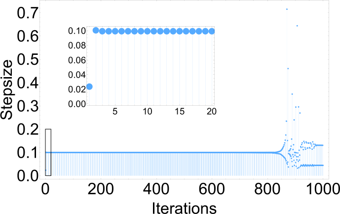
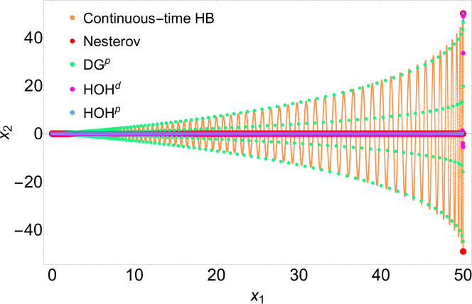
Figure 1: Ill-conditioned quadratic objective function example. (a) Evolution of the stepsize along the execution of HOH${}^{\operatorname{p}}$ during the first $1000$ iterations. (b) State evolution along DG${}^{\operatorname{p}}$, HOH${}^{\operatorname{d}}$, HOH${}^{\operatorname{p}}$, continuous heavy-ball dynamics, and Nesterov’s method starting from $x=(50,50)$ and $v=(-0.0023,-4.7139)$.

Figure 1(b) compares the performance of DG${}^{\operatorname{p}}$, HOH${}^{\operatorname{d}}$, and HOH${}^{\operatorname{p}}$ against the continuous heavy-ball method and the discrete Nesterov method for strongly convex functions. The DG${}^{\operatorname{p}}$ algorithm takes large stepsizes following the evolution of the continuous heavy-ball along the straight lines $p(t)=p_{k}+tX_{\operatorname{hb}}^{a}(p_{k})$. Meanwhile, the higher-order nature of the hold employed by HOH${}^{\operatorname{d}}$ and HOH${}^{\operatorname{p}}$ makes them able to leap over the oscillations, yielding a state evolution similar to Nesterov’s method. Figure 2 shows the evolution of the objective and Lyapunov functions. We observe that after some initial iterations, HOH${}^{\operatorname{p}}$ outperforms Nesterov’s method. Eventually, also DG${}^{\operatorname{p}}$ catches up to Nesterov’s method.

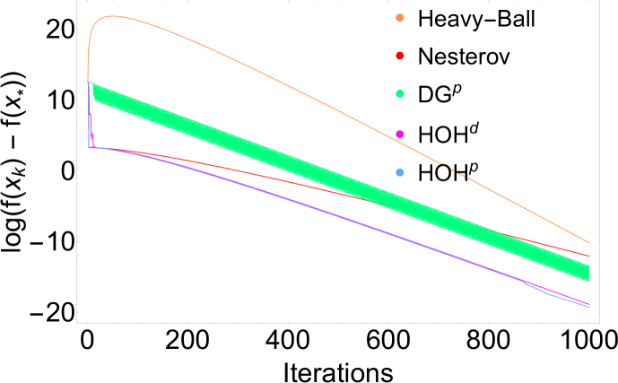
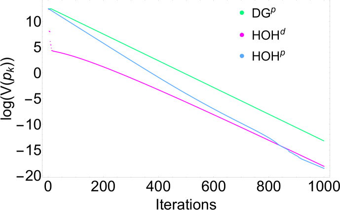
Figure 2: Ill-conditioned quadratic objective function example. (a) Evolution of the logarithm of the objective function under DG${}^{\operatorname{p}}$, HOH${}^{\operatorname{d}}$, HOH${}^{\operatorname{p}}$, the heavy-ball method, and Nesterov’s method starting from $x=(50,50)$ and $v=(-0.0023,-4.7139)$. (b) Corresponding evolution of the logarithm of the Lyapunov function along DG${}^{\operatorname{p}}$, HOH${}^{\operatorname{d}}$, and HOH${}^{\operatorname{p}}$.

Logarithmic Regression

Consider the optimization of the regularized logistic regression cost function $f:{\mathbb{R}}^{4}\rightarrow{\mathbb{R}}$ defined by $f(x)=\sum_{i=1}^{10}\log(1+e^{-y_{i}\langle z_{i},x\rangle})+\frac{1}{2}\left\lVert x\right\rVert^{2}$, where the points $\{z_{i}\}_{i=1}^{10}\subset\mathbb{R}^{4}$ are generated randomly using a uniform distribution in the interval $[-5,5]$, and the points $\{y_{i}\}_{i=1}^{10}\subset\{-1,1\}$ are generated similarly with quantized values. This objective function is $1$-strongly convex and one can also compute the value $L=177.49$. We use $a=0.025$ and $s=\mu/(36L^{2})$, and initialize the velocity according to (4b). Figure 3(a) and (b) show the evolution of the stepsize along HOH${}^{\operatorname{p}}$, which changes as a function of the state looking to satisfy the desired decay of the Lyapunov function.

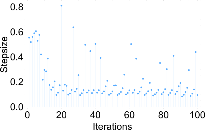
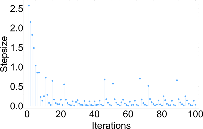
Figure 3: Logarithmic regression example. (a) Evolution of the stepsize along the execution of HOH${}^{\operatorname{p}}$ starting from $x=(50,50,50,50)$ and $v=(-0.1026,-0.09265,-0.1078,-0.0899)$. Notice the complex pattern, with significant increases and oscillations along the trajectory. (b) Difference between the optimal stepsize (computed using the exact Lyapunov function, which assumes knowledge of the minimizer) and the stepsize of HOH${}^{\operatorname{p}}$. The largest difference is achieved at the beginning: after a few iterations, the difference descreases significantly, periodically becoming almost zero.

Figure 4 shows the evolution of the objective and Lyapunov functions. We observe how HOH${}^{\operatorname{d}}$ and HOH${}^{\operatorname{p}}$ outperform Nesterov’s method, although eventually the heavy-ball algorithm performs the best. The Lyapunov function decreases at a much faster rate along HOH${}^{\operatorname{d}}$ and HOH${}^{\operatorname{p}}$ than along DG${}^{\operatorname{p}}$.

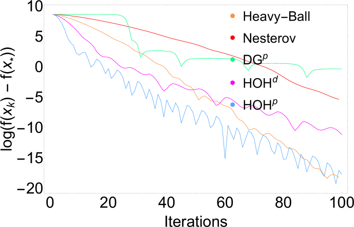
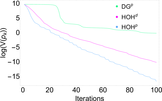
Figure 4: Logarithmic regression example. (a) Evolution of the logarithm of the objective function under DG${}^{\operatorname{p}}$, HOH${}^{\operatorname{d}}$, HOH${}^{\operatorname{p}}$, the heavy-ball method, and Nesterov’s method starting from $x=(50,50,50,50)$ and $v=(-0.1026,-0.09265,-0.1078,-0.0899)$. (b) Corresponding evolution of the logarithm of the Lyapunov function along DG${}^{\operatorname{p}}$, HOH${}^{\operatorname{d}}$, and HOH${}^{\operatorname{p}}$.

VII Conclusions

We have introduced a resource-aware control framework to the discretization of accelerated optimization flows that specifically takes advantage of their dynamical properties. We have exploited fundamental concepts from opportunistic state-triggering related to the various ways of encoding the notion of valid Lyapunov certificates, the use of sampled-data information, and the construction of state estimators and holders to synthesize variable-stepsize optimization algorithms that retain by design the convergence properties of their continuous-time counterparts. We believe these results open the way to a number of exciting research directions. Among them, we highlight the design of adaptive learning schemes to refine the use of sampled data and optimize the algorithm performance with regards to the objective function, the characterization of accelerated convergence rates, employing tools and insights from hybrid systems for analysis and design, enriching the proposed designs by incorporating re-start schemes as triggering conditions to avoid overshooting and oscillations, and developing distributed implementations for network optimization problems.

Appendix A

Throughout the appendix, we make use of a number of basic facts that we gather here for convenience,

$$f(x_{*})-f(x) \leq-\frac{\left\lVert\nabla f(x)\right\rVert^{2}}{2L}$$ (A.1a)

$$\frac{\left\lVert\nabla f(x)\right\rVert}{L}\leq\left\lVert x-x_{*}\right\rVert \leq\frac{\left\lVert\nabla f(x)\right\rVert}{\mu}$$ (A.1b)

$$f(y)-f(x)-\langle\nabla f(x),y-x\rangle \leq\frac{L}{2}\left\lVert y-x\right\rVert^{2}$$ (A.1c)

$$\frac{1}{L}\left\lVert\nabla f(x)-\nabla f(y)\right\rVert^{2} \leq\langle\nabla f(x)-\nabla f(y),x-y\rangle$$ (A.1d)

$$f(y)-f(x)-\langle\nabla f(x),y-x\rangle \leq\frac{1}{2\mu}\left\lVert\nabla f(y)-\nabla f(x)\right\rVert^{2}$$ (A.1e)

We also resort at various points to the expression of the gradient of $V$,

$$\nabla V(p) =\begin{bmatrix}\sqrt{\mu_{s}}\nabla f(x)+\sqrt{\mu}v+2\mu(x-x_{*})\\ v+\sqrt{\mu}(x-x_{*})\end{bmatrix}.$$ (A.2)

The following result is used in the proof of Theorem IV.2.

Lemma A.1.

For $\beta_{1},\dots,\beta_{4}>0$, the function

$$g(z)=\frac{\beta_{3}+\beta_{4}z^{2}}{-\beta_{1}+\beta_{2}z}$$ (A.3)

is positively lower bounded on $(\beta_{1}/\beta_{2},\infty)$.

Proof.

The derivative of $g$ is

$$g^{\prime}(z)=\frac{-\beta_{2}\beta_{3}+\beta_{4}z(-2\beta_{1}+\beta_{2}z)}{(\beta_{1}-\beta_{2}z)^{2}}.$$

The solutions to $g^{\prime}(z)=0$ are then given by

$$z_{\operatorname{root}}^{\pm}=\frac{\beta_{1}\beta_{4}\pm\sqrt{\beta_{2}^{2}\beta_{3}\beta_{4}+\beta_{1}^{2}\beta_{4}^{2}}}{\beta_{2}\beta_{4}}.$$ (A.4)

Note that $z^{-}_{\operatorname{root}}<0<\beta_{1}/\beta_{2}<z^{+}_{\operatorname{root}}$, $g^{\prime}$ is negative on $(z^{-}_{\operatorname{root}},z^{+}_{\operatorname{root}})$, and positive on $(z^{+}_{\operatorname{root}},\infty)$. Therefore the minimum value over $(\beta_{1}/\beta_{2},\infty)$ is achieved at $z^{+}_{\operatorname{root}}$, and corresponds to $g(z^{+}_{\operatorname{root}})>0$. ∎

Proof of Proposition IV.4.

We break out $\frac{d}{dt}V(p(t))+\frac{\sqrt{\mu}}{4}V({p}(t))$ as follows

$$\frac{d}{dt}V(\hat{p}+tX_{\operatorname{hb}}^{a}(\hat{p}))+\frac{\sqrt{\mu}}{4}V(\hat{p}+tX_{\operatorname{hb}}^{a}(\hat{p}))=$$

$$=\underbrace{\langle\nabla V(\hat{p}),X_{\operatorname{hb}}^{a}(\hat{p})\rangle+\frac{\sqrt{\mu}}{4}V(\hat{p})}_{\textrm{Term I + II + III}}$$

$$\quad+\underbrace{\langle\nabla V(\hat{p}+tX_{\operatorname{hb}}^{a}(\hat{p}))-\nabla V(\hat{p}),X_{\operatorname{hb}}^{a}(\hat{p})\rangle}_{\textrm{Term IV + V}}$$

$$\quad+\frac{\sqrt{\mu}}{4}(\underbrace{V(\hat{p}+tX_{\operatorname{hb}}^{a}(\hat{p}))-V(\hat{p})}_{\textrm{Term VI}}),$$

and bound each term separately.

$\mathbf{Term\ I+II+III}$. From the definition (III.1) of $V$ and the fact that $\left\lVert y_{1}+y_{2}\right\rVert^{2}\leq 2\left\lVert y_{1}\right\rVert^{2}+2\left\lVert y_{2}\right\rVert^{2}$, we have

$$V(\hat{p}) =\sqrt{\mu_{s}}(f(\hat{x})-f(x_{*}))+\frac{1}{4}\left\lVert\hat{v}\right\rVert^{2}$$

$$\quad+\frac{1}{4}\left\lVert\hat{v}+2\sqrt{\mu}(\hat{x}-x_{*})\right\rVert^{2}$$

$$\leq\sqrt{\mu_{s}}(f(\hat{x})-f(x_{*}))$$

$$\quad+\frac{1}{4}\left\lVert\hat{v}\right\rVert^{2}+\frac{2}{4}\left\lVert\hat{v}\right\rVert^{2}+\frac{2}{4}\left\lVert 2\sqrt{\mu}(\hat{x}-x_{*})\right\rVert^{2}$$

$$=\sqrt{\mu_{s}}(f(\hat{x})-f(x_{*}))+\frac{3}{4}\left\lVert\hat{v}\right\rVert^{2}+2\mu\left\lVert\hat{x}-x_{*}\right\rVert^{2}.$$

Using this bound, we obtain

$$\langle\nabla V(\hat{p}),X^{a}_{\operatorname{hb}}(\hat{p})\rangle+\frac{\sqrt{\mu}}{4}V(\hat{p})$$

$$\leq-\sqrt{\mu}\left\lVert\hat{v}\right\rVert^{2}+\frac{\sqrt{\mu}}{4}\sqrt{\mu_{s}}(f(\hat{x})-f(x_{*}))+\frac{3\sqrt{\mu}}{16}\left\lVert\hat{v}\right\rVert^{2}$$

$$\quad+\frac{\mu\sqrt{\mu}}{2}\left\lVert\hat{x}-x_{*}\right\rVert^{2}+\sqrt{\mu_{s}}\langle\nabla f(\hat{x})-\nabla f(\hat{x}+a\hat{v}),\hat{v}\rangle$$

$$\quad-\sqrt{\mu}\sqrt{\mu_{s}}\langle\nabla f(\hat{x}+a\hat{v}),\hat{x}-x_{*}\rangle.$$

Writing $0$ as $0=a\hat{v}-a\hat{v}$ and using strong convexity, we can upper bound $\langle\nabla f(\hat{x}+a\hat{v}),x_{*}-\hat{x}\rangle$ in the last summand by the expression

$$f(x_{*})-f(\hat{x}+a\hat{v})-\frac{\mu}{2}\left\lVert\hat{x}+a\hat{v}-x_{*}\right\rVert^{2}+\langle\nabla f(\hat{x}+a\hat{v}),a\hat{v}\rangle.$$

Substituting this bound above and re-grouping terms,

$$\langle\nabla V(\hat{p}),X^{a}_{\operatorname{hb}}(\hat{p})\rangle+\frac{\sqrt{\mu}}{4}V(\hat{p})\leq-\sqrt{\mu}\left\lVert\hat{v}\right\rVert^{2}$$

$$\quad+\underbrace{\sqrt{\mu}\sqrt{\mu_{s}}\Big{(}\frac{1}{4}(f(\hat{x})-f(x_{*}))+f(x_{*})-f(\hat{x}+a\hat{v})\Big{)}}_{\textrm{(a)}}$$

$$\quad+\frac{3\sqrt{\mu}}{16}\left\lVert\hat{v}\right\rVert^{2}+\sqrt{\mu_{s}}\langle\nabla f(\hat{x})-\nabla f(\hat{x}+a\hat{v}),\hat{v}\rangle$$

$$\quad\underbrace{+\frac{\mu\sqrt{\mu}}{2}\left\lVert\hat{x}-x_{*}\right\rVert^{2}+\sqrt{\mu}\sqrt{\mu_{s}}(-\frac{\mu}{2}\left\lVert\hat{x}+a\hat{v}-x_{*}\right\rVert^{2})}_{\textrm{(b)}}$$

$$\quad+\sqrt{\mu}\sqrt{\mu_{s}}\langle\nabla f(\hat{x}+a\hat{v}),a\hat{v}\rangle.$$

Observe that

(a) $$=\sqrt{\mu}\sqrt{\mu_{s}}\big{(}-\frac{3}{4}(f(\hat{x})-f(x_{*}))+f(\hat{x})-f(\hat{x}+a\hat{v})\big{)},$$

(b) $$\leq-\frac{\mu^{2}\sqrt{s}}{2}\left\lVert\hat{x}-x_{*}\right\rVert^{2}+\sqrt{\mu_{s}}\mu^{3/2}\left\lVert\hat{x}-x_{*}\right\rVert\left\lVert a\hat{v}\right\rVert$$

$$\quad-\sqrt{\mu_{s}}\mu^{3/2}/2\left\lVert a\hat{v}\right\rVert^{2},$$

where, in the expression of (a), we have expressed $0$ as $0=3/4(f(\hat{x})-f(\hat{x}))$ and, in the expression of (b), we have expanded the square and used the Cauchy-Schwartz inequality [31]. Finally, resorting to (A.1), we obtain

$$\langle\nabla V(\hat{p}),X^{a}_{\operatorname{hb}}(\hat{p})\rangle+\frac{\sqrt{\mu}}{4}V(\hat{p})\leq C_{\operatorname{ET}}(\hat{p};a)=C_{\operatorname{ST}}(\hat{p};a).$$

$\bullet$ $\mathbf{Term\ IV+V}$. Using (A.2) we have

$$\nabla V(\hat{p}+tX_{\operatorname{hb}}^{a}(\hat{p}))=$$

$$\begin{bmatrix}\sqrt{\mu_{s}}\nabla f(\hat{x}+t\hat{v})+\sqrt{\mu}\hat{v}-2\mu t\hat{v}\\ -t\sqrt{\mu}\sqrt{\mu_{s}}\nabla f(\hat{x}+a\hat{v})+2\mu(\hat{x}+t\hat{v}-x_{*})\\ \vskip 6.0pt plus 2.0pt minus 2.0pt\cr\hat{v}-2t\sqrt{\mu}\hat{v}-t\sqrt{\mu_{s}}\nabla f(\hat{x}+a\hat{v})+\sqrt{\mu}(\hat{x}+t\hat{v}-x_{*})\end{bmatrix}.$$

Therefore, $\nabla V(\hat{p}+tX_{\operatorname{hb}}^{a}(\hat{p}))-\nabla V(\hat{p})$ reads

$$\begin{bmatrix}\sqrt{\mu_{s}}(\nabla f(\hat{x}\!+\!t\hat{v})\!-\!\nabla f(\hat{x}))\!-\!t\sqrt{\mu}\sqrt{\mu_{s}}\nabla f(\hat{x}\!+\!a\hat{v})\\ \vskip 6.0pt plus 2.0pt minus 2.0pt\cr-\sqrt{\mu}t\hat{v}-t\sqrt{\mu_{s}}\nabla f(\hat{x}+a\hat{v})\end{bmatrix}$$

and hence

$$\langle\nabla V(\hat{p}+tX_{\operatorname{hb}}^{a}(\hat{p}))-\nabla V(\hat{p}),X_{\operatorname{hb}}^{a}(\hat{p})\rangle$$

$$=\sqrt{\mu_{s}}\langle\nabla f(\hat{x}+t\hat{v})-\nabla f(\hat{x}),\hat{v}\rangle$$

$$\quad+2t\sqrt{\mu}\sqrt{\mu_{s}}\langle\nabla f(\hat{x}+a\hat{v}),\hat{v}\rangle+2t\mu\left\lVert\hat{v}\right\rVert^{2}$$

$$\quad+t\mu_{s}\left\lVert\nabla f(\hat{x}+a\hat{v})\right\rVert^{2}.$$

The RHS of the last expression is precisely $A_{\operatorname{ET}}(\hat{p},t;a)$. Using the $L$-Lipschitzness of $\nabla f$, one can see that $A_{\operatorname{ET}}(\hat{p},t;a)\leq A_{\operatorname{ST}}(p;a)t$.

$\bullet$ $\mathbf{Term\ VI}$. From (III.1),

$$V(\hat{p}+tX_{\operatorname{hb}}^{a}(\hat{p}))-V(\hat{p})=\sqrt{\mu_{s}}(f(\hat{x}+t\hat{v})-f(x_{*}))$$

$$\quad+\frac{1}{4}\left\lVert\hat{v}-2t\sqrt{\mu}\hat{v}-t\sqrt{\mu_{s}}\nabla f(\hat{x}+a\hat{v})\right\rVert^{2}$$

$$\quad+\frac{1}{4}\left\lVert\hat{v}\right.-2t\sqrt{\mu}\hat{v}-t\sqrt{\mu_{s}}\nabla f(\hat{x}+a\hat{v})$$

$$\quad+\left.2\sqrt{\mu}(\hat{x}+t\hat{v}-x_{*})\right\rVert^{2}-\sqrt{\mu_{s}}(f(\hat{x})-f(x_{*}))$$

$$\quad-\frac{1}{4}\left\lVert\hat{v}\right\rVert^{2}-\frac{1}{4}\left\lVert\hat{v}+2\sqrt{\mu}(\hat{x}-x_{*})\right\rVert^{2}.$$

Expanding the squares in the second and third summands, and simplifying, we obtain

$$V(\hat{p}+tX_{\operatorname{hb}}^{a}(\hat{p}))-V(\hat{p})=\sqrt{\mu_{s}}(f(\hat{x}+t\hat{v})-f(\hat{x}))$$

$$\quad+\frac{1}{4}\left\lVert-2t\sqrt{\mu}\hat{v}-t\sqrt{\mu_{s}}\nabla f(\hat{x}+a\hat{v})\right\rVert^{2}$$

$$\quad+\frac{1}{2}\langle\hat{v},-2t\sqrt{\mu}\hat{v}-t\sqrt{\mu_{s}}\nabla f(\hat{x}+a\hat{v})\rangle$$

$$\quad+\frac{1}{4}\left\lVert-t\sqrt{\mu_{s}}\nabla f(\hat{x}+a\hat{v})\right\rVert^{2}$$

$$\quad+\frac{1}{2}\langle\hat{v}+2\sqrt{\mu}(\hat{x}-x_{*}),-t(\sqrt{\mu_{s}}\nabla f(\hat{x}+a\hat{v})\rangle$$

$$=\sqrt{\mu_{s}}(f(\hat{x}+t\hat{v})-f(\hat{x}))$$

$$\quad+\frac{1}{4}\left\lVert-2t\sqrt{\mu}\hat{v}-t\sqrt{\mu_{s}}\nabla f(\hat{x}+a\hat{v})\right\rVert^{2}$$

$$\quad-t\sqrt{\mu}\left\lVert\hat{v}\right\rVert^{2}-t\sqrt{\mu_{s}}\langle\hat{v},\nabla f(\hat{x}+a\hat{v})\rangle$$

$$\quad+\frac{1}{4}\left\lVert-t\sqrt{\mu_{s}}\nabla f(\hat{x}+a\hat{v})\right\rVert^{2}$$

$$\quad+\langle\sqrt{\mu}(\hat{x}-x_{*}),-t\sqrt{\mu_{s}}\nabla f(\hat{x}+a\hat{v})\rangle.$$

Note that

$$\langle x_{*}-\hat{x},\nabla f(\hat{x}+a\hat{v})\rangle$$

$$=\langle x_{*}-\hat{x}-av,\nabla f(\hat{x}+a\hat{v})\rangle+\langle a\hat{v},\nabla f(\hat{x}+a\hat{v})\rangle$$

$$\leq-\frac{\left\lVert\nabla f(\hat{x}+a\hat{v})\right\rVert^{2}}{L}+\langle a\hat{v},\nabla f(\hat{x}+a\hat{v})\rangle,$$

where in the inequality we have used (A.1d) with $x=\hat{x}+a\hat{v}$ and $y=x_{*}$. Using this in the equation above, one identifies the expression of $B_{\operatorname{ET}}(p,t;a)$. Finally, applying (A.1c), one can show that $B_{\operatorname{ET}}(p,t;a)\leq B_{\operatorname{ST}}^{l}(p;a)t+B^{q}_{\operatorname{ST}}(p;a)t^{2}$, concluding the proof. ∎

Proof of Proposition V.2.

For convenience, let

$$X_{\operatorname{hb}}^{a,\hat{p}}(p) =\begin{bmatrix}v\\ -2\sqrt{\mu}v-\sqrt{\mu_{s}}\nabla f(\hat{x}+a\hat{v})\end{bmatrix},$$

where $\hat{p}=[\hat{x},\hat{v}]$. We next provide a bound for the expression

$$\frac{d}{dt}V(p(t)))+\frac{\sqrt{\mu}}{4}V(p(t))=\underbrace{\langle\nabla V(\hat{p}),X_{\operatorname{hb}}^{a,\hat{p}}(\hat{p})\rangle+\frac{\sqrt{\mu}}{4}V(\hat{p})}_{\textrm{Term I + II + III}}$$

$$\quad+\underbrace{\langle\nabla V(p(t))-\nabla V(\hat{p}),X_{\operatorname{hb}}^{a,\hat{p}}(p(t))\rangle}_{\textrm{Term IV}}$$

$$\quad+\underbrace{\langle\nabla V(\hat{p}),X_{\operatorname{hb}}^{a,\hat{p}}(p(t))-X_{\operatorname{hb}}^{a,\hat{p}}(\hat{p})\rangle}_{\textrm{Term V}}+\frac{\sqrt{\mu}}{4}\underbrace{(V(p(t))-V(\hat{p}))}_{\textrm{Term VI}}.$$

Next, we bound each term separately.

$\bullet$ $\mathbf{Term\ I+II+III}$. Since $X_{\operatorname{hb}}^{a,\hat{p}}(\hat{p})=X_{\operatorname{hb}}^{a}(\hat{p})$, this term is exactly the same as Term I + II + III in the proof of Proposition IV.4, and hence the bound obtained there is valid.

$\bullet$ $\mathbf{Term\ IV}$. Using (A.2), we have

$$\langle\nabla V(p(t))-\nabla V(\hat{p}),X_{\operatorname{hb}}^{a,\hat{p}}(p(t))\rangle$$

$$=\sqrt{\mu_{s}}\langle\nabla f(x(t))-\nabla f(\hat{x}),v(t)\rangle$$

$$\quad+\sqrt{\mu}\langle v(t)-\hat{v},v(t)\rangle+2\mu\langle x(t)-\hat{x},v(t)\rangle$$

$$\quad-2\sqrt{\mu}\langle v(t)-\hat{v},v(t)\rangle-\sqrt{\mu_{s}}\langle v(t)-\hat{v},\nabla f(\hat{x}+a\hat{v})\rangle$$

$$\quad-2\mu\langle x(t)-\hat{x},v(t)\rangle-\sqrt{\mu_{s}}\sqrt{\mu}\langle x(t)-\hat{x},\nabla f(\hat{x}+a\hat{v})\rangle$$

$$=\sqrt{\mu_{s}}\langle\nabla f(x(t))-\nabla f(\hat{x}),v(t)\rangle-\sqrt{\mu}\langle v(t)-\hat{v},v(t)\rangle$$

$$\quad-\sqrt{\mu_{s}}\langle v(t)-\hat{v},\nabla f(\hat{x}+a\hat{v})\rangle$$

$$\quad-\sqrt{\mu_{s}}\sqrt{\mu}\langle x(t)-\hat{x},\nabla f(\hat{x}+a\hat{v})\rangle,$$

from where we obtain $\mathrm{Term\ IV}\leq\mathfrak{A}_{\operatorname{ET}}(\hat{p},t;a)$. Now, using $0=\hat{v}-\hat{v}$, the $L$-Lipschitzness of $\nabla f$, and the Cauchy-Schwartz inequality, we have

$$|\mathfrak{A}_{\operatorname{ET}}(\hat{p},t;a)| \leq\sqrt{\mu_{s}}L\left\lVert x(t)-\hat{x}\right\rVert(\left\lVert v(t)-\hat{v}\right\rVert+\left\lVert\hat{v}\right\rVert)$$

$$\quad+\sqrt{\mu}\left\lVert v(t)-\hat{v}\right\rVert^{2}+\sqrt{\mu}\left\lVert v(t)-\hat{v}\right\rVert\left\lVert\hat{v}\right\rVert$$

$$\quad+\sqrt{\mu_{s}}\left\lVert v(t)-\hat{v}\right\rVert\left\lVert\nabla f(\hat{x}+a\hat{v})\right\rVert$$

$$\quad+\sqrt{\mu_{s}}\sqrt{\mu}\left\lVert x(t)-\hat{x}\right\rVert\left\lVert\nabla f(\hat{x}+a\hat{v})\right\rVert.$$

Using (20), the triangle inequality, and $1-e^{-2\sqrt{\mu}t}\leq 2\sqrt{\mu}t$, we can write

$$\left\lVert x(t)-\hat{x}\right\rVert \leq\frac{t}{2\sqrt{\mu}}\left\lVert 2\sqrt{\mu}\hat{v}+\sqrt{\mu_{s}}\nabla f(\hat{x}+a\hat{v})\right\rVert$$

$$\quad+\frac{\sqrt{\mu_{s}}t}{2\sqrt{\mu}}\left\lVert\nabla f(\hat{x}+a\hat{v})\right\rVert,$$ (A.5a)

$$\left\lVert v(t)-\hat{v}\right\rVert \leq t\left\lVert 2\sqrt{\mu}\hat{v}+\sqrt{\mu_{s}}\nabla f(\hat{x}+a\hat{v})\right\rVert.$$ (A.5b)

Substituting into the bound for $|\mathfrak{A}_{\operatorname{ET}}(\hat{p},t;a)|$ above, we obtain

$$|\mathfrak{A}_{\operatorname{ET}}(\hat{p},t;a)|\leq\mathfrak{A}^{q}_{ST}(\hat{p};a)t^{2}+\mathfrak{A}_{\operatorname{ST}}^{l}(\hat{p};a)t$$

as claimed.

$\bullet$ $\mathbf{Term\ V}$. Using (A.2), we have

$$\Big{\langle}\nabla V(\hat{p}),X_{\operatorname{hb}}^{a,\hat{p}}(p(t))-X_{\operatorname{hb}}^{a,\hat{p}}(\hat{p})\Big{\rangle}$$

$$=\langle\begin{bmatrix}\sqrt{\mu_{s}}\nabla f(\hat{x})+\sqrt{\mu}\hat{v}+2\mu(\hat{x}-x_{*})\\ \hat{v}+\sqrt{\mu}(\hat{x}-x_{*})\end{bmatrix},$$

$$\quad\begin{bmatrix}v(t)-\hat{v}\\ -2\sqrt{\mu}(v(t)-\hat{v})\end{bmatrix}\rangle$$

$$=\sqrt{\mu_{s}}\langle\nabla f(\hat{x}),v(t)-\hat{v}\rangle+\sqrt{\mu}\langle\hat{v},v(t)-\hat{v}\rangle$$

$$\quad+2\mu\langle\hat{x}-x_{*},v(t)-\hat{v}\rangle-2\sqrt{\mu}\langle\hat{v},v(t)-\hat{v}\rangle$$

$$\quad-2\mu\langle\hat{x}-x_{*},v(t)-\hat{v}\rangle=\mathfrak{D}_{\operatorname{ET}}(\hat{p},t;a).$$

Taking the absolute value and using the Cauchy-Schwartz inequality in conjunction with (A.5), we obtain the expression corresponding to $\mathfrak{D}_{\operatorname{ST}}$.

$\bullet$ $\mathbf{Term\ VI}$. From (III.1),

$$V(p(t))-V(\hat{p})=\sqrt{\mu_{s}}(f(x(t))-f(x_{*}))+\frac{1}{4}\left\lVert v(t)\right\rVert^{2}$$

$$\quad+\frac{1}{4}\left\lVert v(t)+2\sqrt{\mu}(x(t)-x_{*})\right\rVert^{2}$$

$$\quad-\sqrt{\mu_{s}}(f(\hat{x})-f(x_{*}))-\frac{1}{4}\left\lVert\hat{v}\right\rVert^{2}$$

$$\quad-\frac{1}{4}\left\lVert\hat{v}+2\sqrt{\mu}(\hat{x}-x_{*})\right\rVert^{2}.$$

Expanding the third summand (using $x(t)=\hat{x}+(x(t)-\hat{x})$ and $v(t)=\hat{v}+(v(t)-\hat{v})$) as $\left\lVert\hat{v}+2\sqrt{\mu}(\hat{x}-x_{*})\right\rVert^{2}+2\langle\hat{v}+2\sqrt{\mu}(\hat{x}-x_{*}),v(t)-\hat{v}+2\sqrt{\mu}(x(t)-\hat{x})\rangle+\left\lVert v(t)-\hat{v}+2\sqrt{\mu}(x(t)-\hat{x})\right\rVert^{2}$, we obtain after simplification

$$V(p(t))-V(\hat{p})=\sqrt{\mu_{s}}(f(x(t))-f(\hat{x}))$$ (A.6)

$$\quad+\frac{1}{4}(\left\lVert v(t)\right\rVert^{2}-\left\lVert\hat{v}\right\rVert^{2})+\frac{1}{4}\left\lVert v(t)-\hat{v}+2\sqrt{\mu}(x(t)-\hat{x})\right\rVert^{2}$$

$$\quad+\frac{1}{2}\langle v(t)-\hat{v}+2\sqrt{\mu}(x(t)-\hat{x}),\hat{v}+2\sqrt{\mu}(\hat{x}-x_{\ast})\rangle.$$

Using (20), we have

$$\langle v(t)-\hat{v}+2\sqrt{\mu}(x(t)-\hat{x}),2\sqrt{\mu}(\hat{x}-x_{\ast})\rangle$$

$$=-2\sqrt{\mu}\sqrt{\mu_{s}}t\langle\nabla f(\hat{x}+a\hat{v}),\hat{x}-x_{\ast}\rangle$$

$$=-2\sqrt{\mu}\sqrt{\mu_{s}}t\langle\nabla f(\hat{x}+a\hat{v}),\hat{x}+a\hat{v}-x_{\ast}\rangle$$

$$\quad-2\sqrt{\mu}\sqrt{\mu_{s}}t\langle\nabla f(\hat{x}+a\hat{v}),-a\hat{v}\rangle$$

$$\leq-2\sqrt{\mu}\sqrt{\mu_{s}}t\frac{\left\lVert\nabla f(\hat{x}+a\hat{v})\right\rVert^{2}}{L}$$

$$\quad+2\sqrt{\mu}\sqrt{\mu_{s}}t\langle\nabla f(\hat{x}+a\hat{v}),a\hat{v}\rangle,$$

where we have used (A.1d) to derive the inequality. Substituting this bound into (A.6), we obtain $\frac{\sqrt{\mu}}{4}(V(p(t))-V(\hat{p}))\leq\mathfrak{B}_{\operatorname{ET}}(\hat{p},t;a)$. To obtain the $\operatorname{ST}$-expressions, we bound each remaining term separately as follows. Note that

$$f(x(t))-f(\hat{x})\underbrace{\leq}_{\eqref{eq:aux-f}}\langle\nabla f(\hat{x}),x(t)-\hat{x}\rangle+\frac{L^{2}}{2\mu}\left\lVert x(t)-\hat{x}\right\rVert^{2}$$

$$\leq\left\lVert x(t)-\hat{x}\right\rVert\left\lVert\nabla f(\hat{x})\right\rVert+\frac{L^{2}}{2\mu}\left\lVert x(t)-\hat{x}\right\rVert^{2}$$

$$\leq\frac{t}{2\sqrt{\mu}}\left\lVert 2\sqrt{\mu}\hat{v}+\sqrt{\mu_{s}}\nabla f(\hat{x}+a\hat{v})\right\rVert\left\lVert\nabla f(\hat{x})\right\rVert$$

$$\quad+\frac{\sqrt{\mu_{s}}t}{2\sqrt{\mu}}\left\lVert\nabla f(\hat{x}+a\hat{v})\right\rVert\left\lVert\nabla f(\hat{x})\right\rVert$$

$$\quad+\frac{L^{2}}{2\mu}(\frac{t^{2}}{4\mu}\left\lVert 2\sqrt{\mu}\hat{v}+\sqrt{\mu_{s}}\nabla f(\hat{x}+a\hat{v})\right\rVert^{2}$$

$$\quad+\frac{\mu_{s}t^{2}}{4\mu}\left\lVert\nabla f(\hat{x}+a\hat{v})\right\rVert^{2}$$

$$\quad+\frac{\sqrt{\mu_{s}}t^{2}}{2\mu}\left\lVert 2\sqrt{\mu}\hat{v}+\sqrt{\mu_{s}}\nabla f(\hat{x}+a\hat{v})\right\rVert\left\lVert\nabla f(\hat{x}+a\hat{v})\right\rVert),$$

where we have used (A.5a) to obtain the last inequality. Next,

$$\left\lVert v(t)\right\rVert^{2}-\left\lVert\hat{v}\right\rVert^{2}=\left\lVert v(t)-\hat{v}\right\rVert^{2}+2\langle v(t)-\hat{v},\hat{v}\rangle$$

$$\leq t^{2}\left\lVert 2\sqrt{\mu}\hat{v}+\sqrt{\mu_{s}}\nabla f(\hat{x}+a\hat{v})\right\rVert^{2}$$

$$\quad+2t\left\lVert 2\sqrt{\mu}\hat{v}+\sqrt{\mu_{s}}\nabla f(\hat{x}+a\hat{v})\right\rVert\left\lVert\hat{v}\right\rVert,$$

where we have used (A.5b) to obtain the last inequality. Using $\left\lVert y_{1}+y_{2}\right\rVert^{2}\leq 2\left\lVert y_{1}\right\rVert^{2}+2\left\lVert y_{2}\right\rVert^{2}$, we bound

$$\left\lVert v(t)\!-\!\hat{v}\!+\!2\sqrt{\mu}(x(t)\!-\!\hat{x})\right\rVert^{2}\leq 2\left\lVert v(t)\!-\!\hat{v}\right\rVert^{2}\!+\!8\mu\left\lVert x(t)\!-\!\hat{x}\right\rVert^{2}$$

$$\leq 2t^{2}\left\lVert 2\sqrt{\mu}\hat{v}+\sqrt{\mu_{s}}\nabla f(\hat{x}+a\hat{v})\right\rVert^{2}+4\sqrt{\mu}t\cdot$$

$$\quad\cdot\big{(}\left\lVert 2\sqrt{\mu}\hat{v}+\sqrt{\mu_{s}}\nabla f(\hat{x}+a\hat{v})\right\rVert+\sqrt{\mu_{s}}\left\lVert\nabla f(\hat{x}+a\hat{v})\right\rVert\big{)}^{2},$$

where we have used (A.5). Finally,

$$\langle v(t)-\hat{v}+2\sqrt{\mu}(x(t)-\hat{x}),\hat{v}\rangle\leq-\sqrt{\mu_{s}}t\langle\nabla f(\hat{x}+a\hat{v}),\hat{v}\rangle.$$

Employing these bounds in the expression of $\mathfrak{B}_{\operatorname{ET}}$, we obtain $|\mathfrak{B}_{\operatorname{ET}}(\hat{p},t;a)|\leq\mathfrak{B}^{q}_{ST}(\hat{p};a)t^{2}+\mathfrak{B}_{\operatorname{ST}}^{l}(\hat{p};a)t$, as claimed. ∎

Miguel Vaquero was born in Galicia, Spain. He received his Licenciatura and Master’s degree in mathematics from the Universidad de Santiago de Compostela, Spain and the Ph.D. degree in mathematics from Instituto de Ciencias Matemáticas (ICMAT), Spain in $2015$. He was then a postdoctoral scholar working on the ERC project “Invariant Submanifolds in Dynamical Systems and PDE” also at ICMAT. Since October 2017, he has been a postdoctoral scholar at the Department of Mechanical and Aerospace Engineering of UC San Diego. He will start in $2021$ as an Assistant Professor at the School of Human Sciences and Technology of IE University, Madrid, Spain. His interests include optimization, dynamical systems, control theory, machine learning, and geometric mechanics.

Pol Mestres was born in Catalonia, Spain in 1997. He is currently a student of the Bachelor’s Degree in Mathematics and the Bachelor’s Degree in Engineering Physics at Universitat Politècnica de Catalunya, Barcelona, Spain. He was a visiting scholar at University of California, San Diego, CA, USA, from September 2019 to March 2020.

Jorge Cortés (M’02, SM’06, F’14) received the Licenciatura degree in mathematics from Universidad de Zaragoza, Zaragoza, Spain, in 1997, and the Ph.D. degree in engineering mathematics from Universidad Carlos III de Madrid, Madrid, Spain, in 2001. He held postdoctoral positions with the University of Twente, Twente, The Netherlands, and the University of Illinois at Urbana-Champaign, Urbana, IL, USA. He was an Assistant Professor with the Department of Applied Mathematics and Statistics, University of California, Santa Cruz, CA, USA, from 2004 to 2007. He is currently a Professor in the Department of Mechanical and Aerospace Engineering, University of California, San Diego, CA, USA. He is the author of Geometric, Control and Numerical Aspects of Nonholonomic Systems (Springer-Verlag, 2002) and co-author (together with F. Bullo and S. Martínez) of Distributed Control of Robotic Networks (Princeton University Press, 2009). He is a Fellow of IEEE and SIAM. At the IEEE Control Systems Society, he has been a Distinguished Lecturer (2010-2014), and is currently its Director of Operations and an elected member (2018-2020) of its Board of Governors. His current research interests include distributed control and optimization, network science, resource-aware control, nonsmooth analysis, reasoning and decision making under uncertainty, network neuroscience, and multi-agent coordination in robotic, power, and transportation networks.

References

• [1] B. T. Polyak, “Some methods of speeding up the convergence of iterative methods,” USSR Computational Mathematics and Mathematical Physics, vol. 4, no. 5, pp. 1–17, 1964.
• [2] Y. E. Nesterov, “A method of solving a convex programming problem with convergence rate ${O}(1/k^{2})$,” Soviet Mathematics Doklady, vol. 27, no. 2, pp. 372–376, 1983.
• [3] Z. Allen-Zhu and L. Orecchia, “Linear Coupling: An Ultimate Unification of Gradient and Mirror Descent,” in 8th Innovations in Theoretical Computer Science Conference (ITCS 2017), Dagstuhl, Germany, 2017, pp. 1–22.
• [4] B. Hu and L. Lessard, “Dissipativity theory for Nesterov’s accelerated method,” in International Conference on Machine Learning, International Convention Centre, Sydney, Australia, August 2017, pp. 1549–1557.
• [5] L. Lessard, B. Recht, and A. Packard, “Analysis and design of optimization algorithms via integral quadratic constraints,” SIAM Journal on Optimization, vol. 26, no. 1, pp. 57–95, 2016.
• [6] B. V. Scoy, R. A. Freeman, and K. M. Lynch, “The fastest known globally convergent first-order method for minimizing strongly convex functions,” IEEE Control Systems Letters, vol. 2, no. 1, pp. 49–54, 2018.
• [7] S. Bubeck, Y. Lee, and M. Singh, “A geometric alternative to Nesterov’s accelerated gradient descent,” arXiv preprint arXiv:1506.08187, 2015.
• [8] W. Su, S. Boyd, and E. J. Candès, “A differential equation for modeling Nesterov’s accelerated gradient method: theory and insights,” Journal of Machine Learning Research, vol. 17, pp. 1–43, 2016.
• [9] M. Betancourt, M. Jordan, and A. C. Wilson, “On symplectic optimization,” arXiv preprint arXiv: 1802.03653, 2018.
• [10] C. J. Maddison, D. Paulin, Y. W. Teh, B. O’Donoghue, and A. Doucet, “Hamiltonian descent methods,” arXiv preprint arXiv:1809.05042, 2018.
• [11] H. Attouch, Z. Chbani, J. Fadili, and H. Riahi, “First-order optimization algorithms via inertial systems with Hessian driven damping,” arXiv preprint arXiv:1907.10536, 2019.
• [12] B. Shi, S. S. Du, M. I. Jordan, and W. J. Su, “Understanding the acceleration phenomenon via high-resolution differential equations,” arXiv preprint arXiv:1810.08907, 2018.
• [13] B. Sun, J. George, and S. Kia, “High-resolution modeling of the fastest first-order optimization method for strongly convex functions,” arXiv preprint arXiv:2008.11199, 2020.
• [14] R. W. Brockett, “Dynamical systems that sort lists, diagonalize matrices, and solve linear programming problems,” Linear Algebra and its Applications, vol. 146, pp. 79–91, 1991.
• [15] U. Helmke and J. B. Moore, Optimization and Dynamical Systems.   Springer, 1994.
• [16] B. Shi, S. S. Du, M. I. Jordan, and W. J. Su, “Acceleration via symplectic discretization of high-resolution differential equations,” arXiv preprint arXiv:1902.03694, 2019.
• [17] A. Wibisono, A. C. Wilson, and M. I. Jordan, “A variational perspective on accelerated methods in optimization,” Proceedings of the National Academy of Sciences, vol. 113, no. 47, pp. E7351–E7358, 2016.
• [18] A. Wilson, L. Mackey, and A. Wibisono, “Accelerating rescaled gradient descent: Fast optimization of smooth functions,” in Advances in Neural Information Processing Systems, H. Wallach, H. Larochelle, A. Beygelzimer, F. d’Alché Buc, E. Fox, and R. Garnett, Eds., vol. 31.   Curran Associates, Inc., 2019, pp. 13 555–13 565.
• [19] J. Zhang, A. Mokhtari, S. Sra, and A. Jadbabaie, “Direct Runge-Kutta discretization achieves acceleration,” in Advances in Neural Information Processing Systems, S. Bengio, H. Wallach, H. Larochelle, K. Grauman, N. Cesa-Bianchi, and R. Garnett, Eds., vol. 31.   Curran Associates, Inc., 2018, pp. 3900–3909.
• [20] A. C. Wilson, B. Recht, and M. I. Jordan, “A Lyapunov analysis of momentum methods in optimization,” arXiv preprint arXiv:1611.02635, 2018.
• [21] M. Vaquero and J. Cortés, “Convergence-rate-matching discretization of accelerated optimization flows through opportunistic state-triggered control,” in Advances in Neural Information Processing Systems, H. Wallach, H. Larochelle, A. Beygelzimer, F. d’Alché Buc, E. Fox, and R. Garnett, Eds.   Curran Associates, Inc., 2019, vol. 32, pp. 9767–9776.
• [22] A. S. Kolarijani, P. M. Esfahani, and T. Keviczky, “Fast gradient-based methods with exponential rate: a hybrid control framework,” in International Conference on Machine Learning, July 2018, pp. 2728–2736.
• [23] D. Hustig-Schultz and R. G. Sanfelice, “A robust hybrid Heavy-Ball algorithm for optimization with high performance,” in American Control Conference, July 2019, pp. 151–156.
• [24] W. P. M. H. Heemels, K. H. Johansson, and P. Tabuada, “An introduction to event-triggered and self-triggered control,” in IEEE Conf. on Decision and Control, Maui, HI, 2012, pp. 3270–3285.
• [25] C. Nowzari, E. Garcia, and J. Cortés, “Event-triggered control and communication of networked systems for multi-agent consensus,” Automatica, vol. 105, pp. 1–27, 2019.
• [26] P. Ong and J. Cortés, “Event-triggered control design with performance barrier,” in IEEE Conf. on Decision and Control, Miami Beach, FL, Dec. 2018, pp. 951–956.
• [27] M. Laborde and A. Oberman, “A Lyapunov analysis for accelerated gradient methods: From deterministic to stochastic case,” in AISTATS, vol. 108, Online, 2020, pp. 602–612.
• [28] M. Muehlebach and M. Jordan, “A dynamical systems perspective on Nesterov acceleration,” in International Conference on Machine Learning, vol. 97, Long Beach, California, USA, 2019, pp. 4656–4662.
• [29] I. Sutskever, J. Martens, G. Dahl, and G. Hinton, “On the importance of initialization and momentum in deep learning,” in International Conference on Machine Learning, vol. 28, Atlanta, Georgia, USA, 2013, pp. 1139–1147.
• [30] L. Perko, Differential Equations and Dynamical Systems, 3rd ed., ser. Texts in Applied Mathematics.   New York: Springer, 2000, vol. 7.
• [31] S. Lang, Real and Functional Analysis, 3rd ed.   New York: Springer, 1993.