1D planar, cylindrical and spherical subsonic solitary waves in space electron-ion-positive dust plasma systems

Abstract

The space electron-ion-positive dust plasma system containing isothermal inertialess electron species, cold inertial ion species, and stationary positive (positivively charged) dust species is considered. The basic features of one dimensional (1D) planar and nonplanar subsonic solitary waves are investigated by the pseudo-potential and reductive perturbation methods, respectively. It is observed that the presence of the positive dust species reduces the phase speed of the ion-acoustic waves, and consequently supports the subsonic solitary waves with the positive wave potential in such a space dusty plasma system. It is observed that the cylindrical and spherical subsonic solitary waves significantly evolve with time, and that the time evolution of the spherical solitary waves is faster than that of the cylindrical ones. The applications of the work in many space dusty plasma systems, particularly in Earth’s mesosphere, cometary tails, Jupiter’s magnetosphere, etc. are addressed.

The existence of the ion-acoustic (IA) waves in a plasma medium was first predicted first by Tonks and Langmur Tonks29ia-theor on the basis of the fluid dynamics in 1929. The prediction of Tonks and Langmuir Tonks29ia-theor was then verified by Revans Revans33ia-expt in 1933. The well known linear dispersion relation for the IA waves propagating in a pure electron-ion plasma containing cold inertial ion fluid and isothermal inertia-less electron fluid is given by

$$\omega=\frac{kC_{i}}{\sqrt{1+k^{2}\lambda_{D}^{2}}},$$ (1)

where $\omega=2\pi f$ and $k=2\pi/\lambda$ in which $f$ ($\lambda$) is the IA wave frequency (wavelength); $C_{i}=(z_{i}k_{B}T_{e}/m_{i})^{1/2}$ is the IA speed in which $k_{B}$ is the Boltzmann constant, $T_{e}$ is the electron temperature, and $m_{i}$ is the ion mass; $\lambda_{D}=(k_{B}T_{e}/4\pi z_{i}^{2}n_{i0}e^{2})^{1/2}$ is the IA wave-length scale in which $n_{i0}$ ($z_{i}$) is the number density (charge state) of the ion species at equilibrium, and $e$ is the magnitude of the charge of an electron. We note that for a pure electron-ion plasma $n_{e0}=z_{i}n_{i0}$ at equilibrium, where $n_{e0}$ is the electron number density at equilibrium. The dispersion relation (1) becomes $\omega\simeq kC_{i}$ for a long-wavelength limit, $\lambda\gg\lambda_{D}$, and $\omega\simeq\omega_{pi}$ for a short wavelength limit, $\lambda\ll\lambda_{D}$, where $\omega_{pi}=(4\pi z_{i}^{2}n_{i0}e^{2}/m_{i})^{1/2}$ is the angular frequency of ion plasma oscillations. Thus, the angular frequency range of the IA waves is $0>\omega>\omega_{pi}$.

The IA waves Tonks29ia-theor ; Revans33ia-expt are found to be modified in an electron-ion-negative dust plasma system theoretically Shukla92-dia ; DAngelo93-dia ; DAngelo94-dia as well as experimentally Barkan96dia-expt ; Merlino98dia-expt ; Merlino04-dia-expt . It has been found that the increase in number density and charge of the negative dust species enhances the phase speed of the IA waves, and consequently support the supersonic Bharuthram92so-dia ; Popel95so-dia ; Nakamura01so-dia-observ ; Mamun02 ; Mamun08 ; Mamun09 solitary waves (SWs).

There are many space plasma environments, viz. Earth’s mesosphere Havnes96 ; Gelinas98 ; Mendis04 , cometary tails Horanyi96 , Jupiter’s surroundings Tsintikidis96 , Jupiter’s magnetosphere Horanyi93 , etc. where in addition to electron-ion plasmas, positive dust species have been observed Havnes96 ; Gelinas98 ; Mendis04 ; Horanyi96 ; Tsintikidis96 ; Horanyi93 . There are three principal mechanisms by which the dust species becomes positively charged Chow93 ; Rosenberg95 ; Rosenberg96 ; Fortov98 . These are photo-emission of electrons from the dust surface induced by the flux of photons Rosenberg96 , thermionic emission of electrons from the dust grain surface by the radiative heating Rosenberg95 , and secondary emission of electrons from the dust surface by the impact of high energetic plasma particles Chow93 .

The dispersion relation for the IA waves in an electron-ion-positive dust plasma system (containing inertialess isothermal electron species, inertial cold ion species, and stationary positive dust species) is given by

$$\omega=\frac{1}{\sqrt{1+\mu}}\frac{kC_{i}}{\sqrt{1+\frac{1}{1+\mu}k^{2}\lambda_{D}^{2}}},$$ (2)

where $\mu=z_{d}n_{d0}/z_{i}n_{i0}$ with $n_{d}$ ($z_{d}$) being the number density (charge state) of the positive dust species. The dispersion relation (2) becomes $\omega\simeq kC_{i}/(1+\mu)$ for the long-wavelength limit (viz. $\lambda\gg\lambda_{D}$). The dispersion relation $\omega\simeq kC_{i}/\sqrt{1+\mu}$ indicates that the phase speed ($\omega/k)$ decreases with the rise of the value of $\mu$. We note that $\mu=0$ corresponds to the electron-ion plasma Tonks29ia-theor ; Revans33ia-expt , and $\mu\rightarrow\infty$ corresponds to electron-dust plasma Khrapak01 ; Mamun04 . Thus, $0<\mu<\infty$ is valid for the electron-ion-positive dust plasma system.

To investigate the nonlinear propagation of the modified IA (MIA) waves defined by (2), we consider such an electron-ion-positive dust plasma system. The nonlinear dynamics of the MIA waves (2) is described by

$$\frac{\partial n_{i}}{\partial t}+\frac{1}{r^{\nu}}\frac{\partial}{\partial r}(r^{\nu}n_{i}u_{i})=0,$$ (3)

$$\frac{\partial u_{i}}{\partial t}+u_{i}\frac{\partial u_{i}}{\partial x}=-\frac{\partial\phi}{\partial x},$$ (4)

$$\frac{1}{r^{\nu}}\frac{\partial}{\partial r}\left(r^{\nu}\frac{\partial\phi}{\partial r}\right)=(1+\mu)\exp(\phi)-n_{i}-\mu,$$ (5)

where $\nu=0$ for one dimensional (1D) planar geometry and $\nu=1~{}(2)$ for cylindrical (spherical) geometry; the electron species has is assumed to obey the Boltzmann law so that $n_{e}=\exp(\phi)$; $n_{e}$ ($n_{i}$) is the electron (ion) number density normalized by $n_{e0}$ ($n_{i0}$); $u_{i}$ is the ion fluid speed normalized by $C_{i}$; $\phi$ is the electrostatic wave potential normalized by $k_{B}T_{e}/e$; $r$ and $t$ are normalized by $\lambda_{D}$ and $\omega_{pi}^{-1}$, respectively. The assumption of stationary positive dust species is valid because of the mass of the positive dust species being extremely high in comparison with that of the inertial ion species.

To study arbitrary amplitude MIA SWs in planar geometry ($\nu=0$ and $r=x$), we employ the pseudo-potential approach Bernstein57PPA ; Cairns95 by assuming that all dependent variables in (3)$-$(5) depend only on a single variable $\xi=x-{\cal M}t$, where ${\cal M}$ is the Mach number. This transformation and steady state condition allow us to write (3)$-$(5) as

$${\cal M}\frac{dn_{i}}{d\xi}-\frac{d}{d\xi}(n_{i}u_{i})=0,$$ (6)

$${\cal M}\frac{du_{i}}{dl\xi}-u_{i}\frac{du_{i}}{d\xi}=\frac{d\phi}{d\xi},$$ (7)

$$\frac{d^{2}\phi}{d\xi^{2}}=(1+\mu)\exp(\phi)-n_{i}-\mu$$ (8)

The integration of (6) and (7) with respect to $\xi$, and the use of appropriate boundary conditions for localized perturbations (viz. $n_{i}\rightarrow 1$, $u_{i}\rightarrow 0$, and $\phi\rightarrow 0$ at $\xi\rightarrow\pm\infty$) give rise to

$$n_{i}=\frac{1}{\sqrt{1-\frac{2\phi}{{\cal M}^{2}}}}.$$ (9)

Now substituting (9) into (8), and integrating the resulting equation with respect to $\phi$, we obtain an energy integral Bernstein57PPA ; Cairns95 in the form

$$\frac{1}{2}\left(\frac{d\phi}{dx}\right)^{2}+V(\phi)=0,$$ (10)

$$V(\phi)={\cal C}_{0}-(1+\mu)\exp(\phi)-{\cal M}^{2}\sqrt{1-\frac{2\phi}{{\cal M}^{2}}}+\mu\phi.$$ (11)

The integration constant ${\cal C}_{0}\,[=1+\mu+{\cal M}^{2}]$ is chosen under the condition $V(0)=0$. The pseudo-potential $V(\phi)$ allow us to express as

$$\left[V(\phi)\right]_{\phi=0}=0,$$ (12)

$$\left[\frac{dV(\phi)}{d\phi}\right]_{\phi=0}=0,$$ (13)

$$\left[\frac{d^{2}V(\phi)}{d\phi^{2}}\right]_{\phi=0}=\frac{1}{2!}\left[\frac{1}{{\cal M}^{2}}-(1+\mu)\right],$$ (14)

$$\left[\frac{d^{3}V(\phi)}{d\phi^{3}}\right]_{\phi=0}=\frac{1}{3!}\left[\frac{3}{{\cal M}^{4}}-(1+\mu)\right].$$ (15)

It is obvious from (12) and (13) that the MIA SWs exist if and only if $[d^{2}V/d\phi^{2}]_{\phi=0}<0$, which makes the fixed point at the origin is unstable Cairns95 , and that $[d^{3}V/d\phi^{3}]_{\phi=0}\>\,(<)\,0$ for the existence Cairns95 of the MIA SWs with $\phi>0$ ($\phi<0$). The condition $[d^{2}V/d\phi^{2}]_{\phi=0}=0$ yields the critical Mach number ${\cal M}_{c}$ (minimum value of ${calM}$ above which the MIA SWs exist). Thus, from (14) we can define ${\cal M}_{c}$ as

$${\cal M}_{c}=\frac{1}{\sqrt{1+\mu}}.$$ (16)

The variation of ${\cal M}_{c}$ with $\mu$ is graphically shown to find the range of the values of $\mu$ and corresponding ${\cal M}$ for which the subsonic MIA SWs exist. The results are displayed in figure 1.

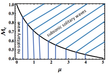
Figure 1: The range of the values of $\mu$ and corresponding ${\cal M}$ for which the subsonic MIA SWs exist.

It is clear from figure 1 that in the region above the curve (indicated by the horizontal lines) the subsonic MIA SWs are formed, and that in the region below the curve (indicated by the vertical lines) no solitary wave exists. On the other hand, $[d^{3}V/d\phi^{3}]_{\phi=0}({\cal M}={\cal M}_{c})=0$ yields ${\cal S}_{c}$: The subsonic MIA SWs with $\phi>0$ ($\phi<0$) exist if ${\cal S}_{c}>0$ (${\cal S}_{c}<0)$, where ${\cal S}_{c}=\mu+2/3$. The latter implies that ${\cal S}_{c}>0$ is always valid since $0<\mu<\infty$, and that the MIA SWs exist only with $\phi>0$ (so, from now ‘SWs’ will be used to mean ‘MIA SWs with $\phi>0$’).

We now plot $V(\phi)$ vs. $\phi$ curves to study the formation of arbitrary amplitude subsonic SWs for which the potential wells are formed in $+\phi$-axis. The numerical results are shown in figures 2 and 3.

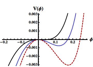
Figure 2: The potential wells corresponding to arbitrary amplitude subsonic SWs for ${\cal M}=0.9$, $\mu=0.1$ (solid curve), $\mu=0.4$ (dotted curve), and $\mu=0.7$ (dashed curve).

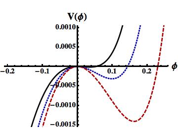
Figure 3: The potential wells corresponding to arbitrary amplitude subsonic SWs for $\mu=0.3$, ${\cal M}=0.90$ (solid curve), ${\cal M}=0.94$ (dotted curve), and ${\cal M}=0.98$ (dashed curve).

The potential wells in $+\phi$ axis in figure 2 or 3 represent the amplitude $\phi_{m}$ (value of $\phi$ at the point where the $V(\phi)$ vis. $\phi$ curve crosses $+\phi$-axis) and the width ${\cal W}$ (defined as ${\cal W}=|\phi_{m}|/\sqrt{|V_{m}|}$, where $|V_{m}|$ is the maximum value of $V(\phi)$ in the potential wells) of arbitrary amplitude SWs. Thus figures 2 and 3 indicate that the amplitude (width) of the subsonic SWs increases (decrease) with the rise of the value of $\mu$ and ${\cal M}$.

We now study the basic features of small amplitude subsonic SWs for which the pseudo-potential $V(\phi)$ [defined by (11)] can be expanded as

$$V(\phi)=C_{2}\phi^{2}+C_{3}\phi^{3}+\cdot\cdot\cdot,$$ (17)

$$C_{2}=\frac{1}{2!}\left[\frac{1}{{\cal M}^{2}}-(1+\mu)\right],$$ (18)

$$C_{3}=\frac{1}{3!}\left[\frac{3}{{\cal M}^{4}}-(1+\mu)\right].$$ (19)

It is clear from (17) that the constant and the coefficient of $\phi$ in the expansion of $V(\phi)$ vanish because of the choice of the integration constant, and the equilibrium charge neutrality condition, respectively. The approximation $V(\phi)=C_{2}\phi^{2}+C_{3}\phi^{3}$, which is valid as long as $C_{n}\phi^{n}$ (where $n=4,~{}5,~{}6,\cdot\cdot\cdot$) are negligible compared to $C_{3}\phi^{3}$), and the condition $V(\phi_{m})=0$ reduce the solitary wave solution of (10) to

$$\phi=\left(-\frac{C_{2}}{C_{3}}\right){\rm sech^{2}}\left(\sqrt{-\frac{C_{2}}{2}}\xi\right).$$ (20)

We have graphically represented (20) for $1>{\cal M}>{\cal M}_{c}$ and $\mu>0$ to observe the basic features of small amplitude subsonic SWs for different values of $\mu$ and ${\cal M}$. The results are displayed in figures 4 and 5.

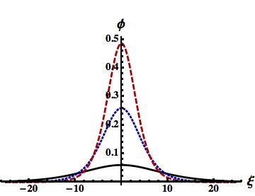
Figure 4: The small amplitude subsonic MIA SWs for ${\cal M}=0.9$, $\mu=0.3$ (solid curve), $\mu=0.4$ (dotted curve), and $\mu=0.7$ (dashed curve).

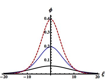
Figure 5: The small amplitude subsonic SWs for $\mu=0.5$, ${\cal M}=0.90$ (solid curve), ${\cal M}=0.94$ (dotted curve), and ${\cal M}=0.98$ (dashed curve).

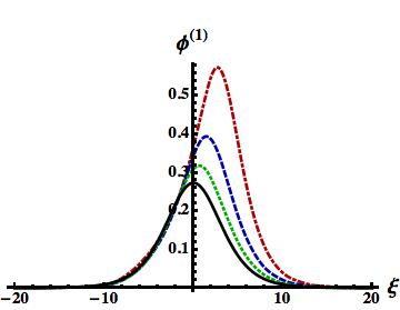
Figure 6: The time evolution of the subsonic SWs in cylindrical ($\nu=1$) geometry for ${\cal U}_{0}=0.1$, $\mu=0.1$, $\tau=-20$ (solid curve), $\tau=-15$ (dotted curve), $\tau=-10$ (dashed curve), and $\tau=-5$ (dot-dashed curve).

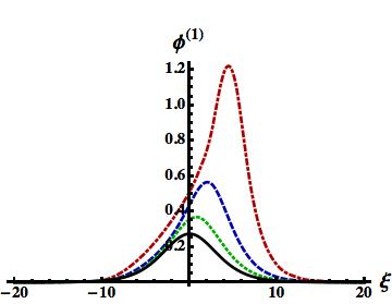
Figure 7: The time evolution of the subsonic SWs in spherical ($\nu=2$) geometry for ${\cal U}_{0}=0.1$, $\mu=0.1$, $\tau=-20$ (solid curve), $\tau=-15$ (dotted curve), $\tau=-10$ (dashed curve), and $\tau=-5$ (dot-dashed curve).

It is obvious from figures 4 and 5 that stationary positive dust species supports the small amplitude subsonic SWs in an electron-ion-positive dust plasma system. The variation of their amplitudes and width with $\mu$ and ${\cal M}$ are obvious from figures 4 and 5. The latter indicate that the amplitude (width) of these subsonic SWs increase (decrease) with the rise of the value of $\mu$ and ${\cal M}$ as we concluded from the direct analysis of the pseudo-potential $V(\phi)$ in figures 2 and 3.

We finally examine the effect of nonplanar geometry on time dependent supersonic SWs by using the reductive perturbation method Washimi66 which requires the stretching the independent variables Maxon74 ; Mamun01 :

$$\zeta=-\epsilon^{\frac{1}{2}}(r+{\cal V}_{p}t),$$ (21)

$$\tau=\epsilon^{\frac{3}{2}}t,$$ (22)

expanding the dependent variables Washimi66 ; Maxon74 ; Mamun01 :

$$n_{i}=1+\epsilon n_{i}^{(1)}+\epsilon^{2}n_{i}^{(2)}+\cdot\cdot\cdot,$$ (23)

$$u_{i}=0+\epsilon u_{i}^{(1)}+\epsilon^{2}u_{i}^{(2)}+\cdot\cdot\cdot,$$ (24)

$$\phi=0+\epsilon\phi^{(1)}+\epsilon^{2}\phi^{(2)}+\cdot\cdot\cdot,$$ (25)

and developing equations in various powers of $\epsilon$. To the lowest order in $\epsilon$, (3)$-$(5) yield

$$n_{i}^{(1)}=-\frac{u_{i}^{(1)}}{{\cal V}_{p}},$$ (26)

$$u_{i}^{(1)}=-\frac{\phi^{(1)}}{{\cal V}_{p}},$$ (27)

$${\cal V}_{p}=\frac{1}{\sqrt{1+\mu}}.$$ (28)

We note that ${\cal V}_{p}={\cal M}_{c}$, and thus the variation of ${\cal V}_{p}$ is shown in figure 1. To the next higher order in $\epsilon$, we obtain a set of equations:

$$\frac{\partial n_{i}^{(1)}}{\partial\tau}-\frac{\partial}{\partial\zeta}\left[{\cal V}_{p}n_{i}^{(2)}+u_{i}^{(2)}+n_{i}^{(1)}u_{i}^{(1)}\right]-\frac{\nu u_{i}^{(1)}}{{\cal V}_{p}\tau}=0,$$ (29)

$$\frac{\partial u_{i}^{(1)}}{\partial\tau}-{\cal V}_{p}\frac{\partial u_{i}^{(2)}}{\partial\zeta}-u_{i}^{(1)}\frac{\partial u_{i}^{(1)}}{\partial\zeta}=\frac{\partial\phi^{(2)}}{\partial\zeta},$$ (30)

$$\frac{\partial^{2}\phi^{(1)}}{\partial\zeta^{2}}=(1+\mu)\phi^{(2)}-n_{i}^{(2)}+\frac{1}{2}(1+\mu)[\phi^{(1)}]^{2}.$$ (31)

The use of (26)$-$(31) gives rise to a modified Korteweg-de Vries (K-dV) equation in the form

$$\frac{\partial\phi^{(1)}}{\partial\tau}+\frac{\nu}{2\tau}\phi^{(1)}+{\cal A}\phi^{(1)}\frac{\partial\phi^{(1)}}{\partial\zeta}+{\cal B}\frac{\partial^{3}\phi^{(1)}}{\partial\zeta^{3}}=0,$$ (32)

where ${\cal A}$ and ${\cal B}$ are nonlinear and dispersion coefficients, and are, respectively, given by

$${\cal A}=\frac{3}{2\sqrt{1+\mu}}\left(\mu+\frac{2}{3}\right),$$ (33)

$${\cal B}=\frac{1}{2(1+\mu)^{\frac{3}{2}}}.$$ (34)

We note that $(\nu/2\tau)\phi^{(1)}$ in (32) is due to the effect of the nonplanar geometry, and that $\nu=0$ or $|\tau|\rightarrow\infty$ corresponds to a 1D planar geometry. Thus, for a large value of $\tau$, and for a frame moving with a speed ${\cal U}_{0}$, the stationary solitary wave solution of (32) is Mamun02

$$\phi^{(1)}=\left(\frac{3{\cal U}_{0}}{{\cal A}}\right){\rm sech^{2}}\left[\sqrt{\frac{u_{0}}{4B}}(\zeta-{\cal U}_{0}\tau)\right].$$ (35)

We note that $\tau<0$ means the time evolution of the SWs from past to present. But we cannot use $\tau\rightarrow 0$ because of the term $(\nu/2\tau)\phi^{(1)}$ in (32).

We now numerically solve (32) to observe how the SWs evolve with time from past to present by using (35) as the initial solitary pulse. The results for cylindrical ($\nu=1$) and spherical ($\nu=2$) geometries are shown in figures 6 and 7, respectively. We note that for a large value of $\tau$ (viz. $\tau=20$) we got solid curves in figures 6 and 7, which represent subsonic SWs in 1D planar, cylindrical, and spherical geometries.

To summarize, we have considered a space dusty plasma system containing electron, ion and positive dust species, and have identified the basic features of the subsonic SWs in such space dusty plasma systems. The results obtained from this theoretical investigation are:

1. The condition $0<\mu<\infty$ causes to form the subsonic SWs with $\phi>0$ in the space plasma systems. This is due to the fact that the phase speed of the MIA waves in such a space plasma systems decreases with the rise of the value of $\mu$.

2. The amplitude (width) of the subsonic SWs increases (decreases) with the rise of the value of $\mu$ because of the decrease in the Mach number with the increase in the value of $\mu$.

3. The amplitude of the subsonic SWs is small because of their existence for low Mach number (${\cal M}<1$).

4. The cylindrical and spherical subsonic solitary waves significantly evolve with time, and that the time evolution of the spherical solitary waves is faster than that of the cylindrical ones. This is due to the time and geometry dependent extra term $(\nu/2\tau)\phi^{(1)}$ in the modified K-dV equation.

The disadvantage of the pseudo-potential method is that it does not allow us to observe the time evolution of the arbitrary amplitude SWs. On the other hand, the reductive perturbation method allows as to observe the time evolution of the small amplitude SWs, but it is not valid for the arbitrary amplitude SWs.

To overcome this limitation, one has to develop a correct numerical code, and to solve the basic equations (3)$-$(5) numerically by this numerical code. This type of numerical analysis will be able to show the time evolution of arbitrary amplitude SWs. This is, of course, a challenging research problem, but beyond the scope of our present work.

We finally hope that the results of this work should be useful for understanding the physics of nonlinear phenomena like subsonic solitary like structures in many space plasma environments, viz. Earth’s mesosphere Havnes96 ; Gelinas98 ; Mendis04 , cometary tails Horanyi96 , Jupiter’s surroundings Tsintikidis96 , Jupiter’s magnetosphere Horanyi93 , etc.

References

- (1) L. Tonks and I. Langmuir, Phy. Rev. 33, 195 (1929).at
- (2) R. W. Revans, Phy. Rev. 44 798 (1933).
- (3) P. K. Shukla an V. P. Silin, Phys. Scr. 45, 508 (1992).
- (4) N. D’Angelo, Planet. Space Sci. 41, 469 (1993).
- (5) N. D’Angelo, Planet. Space Sci. 42, 507 (1994).
- (6) A. Barkan, N. D’Angelo, and R. Merlino, Planet. Space Sci. 44, 239 (1996).
- (7) R. L. Merlino, A. Barkan, C. Thompson, and N. D’Angelo, Phys. Plasmas 5, 1590 (1998).
- (8) R. Merlino and J. Goree, Phys. Today 57 (7), 32 (2004).
- (9) R. Bharuthram and P. K. Shukla, Planet. Space Sci. 40, 973 (1992).
- (10) S. I. Popel and M. Y. Yu, Contrib. Plasma Phys. 35, 103 (1995).
- (11) Y. Nakamura and A. Sharma, Phys. Plasmas 8, 3921 (2001).
- (12) A. A. Mamun and P. K. Shukla, Phys. Plasmas 9, 1468 (2002).
- (13) A. A. Mamun and P. K. Shukla, Phys. Lett. A 372, 1490 (2008).
- (14) A. A. Mamun and P. K. Shukla, Phys. Rev. E 80, 037401 (2009).
- (15) O. Havnes, J. Trøim, T. Blix, W. Mortensen, L. I. Næsheim, E. Thrane, and T. Tønnesen, J. Geophys. Res. 101, 10839 (1996).
- (16) L. J. Gelinas, K. A. Lynch, M. C. Kelley, S. Collins, S. Baker, Q. Zhou, and J. S. Friedman, Geophys. Res. Lett. 25, 4047 (1998).
- (17) D. A. Mendis, Wai-Ho Wong, and M. Rosenberg, Phys. Scripta T113, 141 (2004).
- (18) M. Horányi, Annu. Rev. Astron. Astrophys. 34, 383 (1996).
- (19) D. Tsintikidis, D. A. Gurnett, W. S. Kurth, and L. J. Granroth, Geophys. Res. Lett. 23, 997 (1996).
- (20) M. Horányi, G. E. Morfill, and E. Grün, Nature London 363, 144 (1993).
- (21) V. W. Chow, D. A. Mendis, and M. Rosenberg, J. Geophys. Res. 98, 19065 (1993).
- (22) M. Rosenberg and D. A. Mendis, IEEE Trans. Plasma Sci. 23, 117 (1995).
- (23) M. Rosenberg, D. A. Mendis, and D. P. Sheehan, IEEE Trans. Plasma Sci. 24, 1422 (1996).
- (24) V. E. Fortov, A. P. Nefedov, O. S. Vaulina et al., J. Exp. Theor. Phys. 87, 1087 [Zh. Eksp. Teor. Fiz. 114, 2004] (1998).
- (25) S. A. Khrapak and G. Morfill, Phys. Plasmas 8, 2629 (2001).
- (26) A. A. Mamun and P. K. Shukla, Geophys. Res. Lett. 31, L06808 (2004).
- (27) I. B. Bernstein, G. M. Greene, and M. D. Kruskal, Phys. Rev. 108, 546 (1957).
- (28) R. A. Cairns, A. A. Mamun, R. Bingham, R. Boström, R. O. Dendy, C. M. C. Nairn, and P. K. Shukla, Geophys. Res. Lett. 22, 2709 (1995).
- (29) H. Washimi, and T. Taniuti, Phys. Rev. Lett. 17, 996 (1966).
- (30) S. Maxon and J. Viecelli, Phys. Rev. Lett. 32, 4 (1974).
- (31) A. A. Mamun and P. K. Shukla, Phys. Lett. A 290, 173 (2001).