Explainable boosted linear regression for time series forecasting

Abstract

Time series forecasting involves collecting and analyzing past observations to develop a model to extrapolate such observations into the future. Forecasting of future events is important in many fields to support decision making as it contributes to reducing the future uncertainty. We propose explainable boosted linear regression (EBLR) algorithm for time series forecasting, which is an iterative method that starts with a base model, and explains the model’s errors through regression trees. At each iteration, the path leading to highest error is added as a new variable to the base model. In this regard, our approach can be considered as an improvement over general time series models since it enables incorporating nonlinear features by residuals explanation. More importantly, use of the single rule that contributes to the error most allows for interpretable results. The proposed approach extends to probabilistic forecasting through generating prediction intervals based on the empirical error distribution. We conduct a detailed numerical study with EBLR and compare against various other approaches. We observe that EBLR substantially improves the base model performance through extracted features, and provide a comparable performance to other well established approaches. The interpretability of the model predictions and high predictive accuracy of EBLR makes it a promising method for time series forecasting.

1 Introduction

Time series forecasting has important applications in various domains including energy [17], finance [27] and weather [8]. Accurate forecasts provide insights on the trends in the domain, and serve as inputs to decisions involving future events. For instance, in supply chain operations, sales and demand forecasts of the products are essential for inventory control, production planning and workforce scheduling. Accordingly, effective forecasting tools are directly linked to increased profits and reduced costs.

Quantitative forecasting methods are generally divided into two categories: general time series models and regression-based models. General time series models such as exponential smoothing and autoregressive integrated moving average (ARIMA) are typically derived from the statistical information in the historic data. On the other hand, regression models rely on constructing a relation between independent variables (e.g. features such as previous observations) and dependent variables (e.g. target outcomes). There is a wide range of regression approaches used for time series forecasting including linear regression, ensemble methods and neural networks.

While majority of previous studies on time series prediction focus on point forecasts, many applications benefit from having probabilistic/interval forecasts that can provide information on future uncertainty. For instance, in retail businesses, probabilistic forecasts enable generating different strategies for a range of possible outcomes provided by the forecast intervals. A probabilistic forecast typically consists of upper and lower limits, and the corresponding interval can be taken as a confidence interval around the point forecasts. Standard methods such as exponential smoothing and ARIMA generate probabilistic forecasts through simulations or closed form expressions for the target predictive distribution [9]. Recent studies propose deep learning models for probabilistic forecasting that target predicting the parameters (i.e. mean and variance) of the probability distribution for the next time step, and show performance improvements over standard approaches for large datasets consisting of a high number of time series [33, 35].

In predictive modeling, often times the models are evaluated by measuring their prediction performance obtained using a test set based on metrics such as mean absolute error and mean squared error, disregarding the interpretability of the model predictions. However, interpretable models have certain benefits such as creating a trust toward the model by explicit characterization of the factors’ contribution to the predictions and providing a better scientific understanding of the model. Value of model interpretability has been acknowledged in recent studies, and lead to new avenues for research [2, 21].

Several recent studies on time series forecasting resort to complex deep learning architectures, which typically yield relatively accurate results when the available data is abundant. The drawbacks of such approaches include their computational burden and the black-box nature [33, 35]. In this regard, linear models may provide a good trade-off between accuracy and simplicity. Specifically, linear models with simple mathematical forms are generally preferred for their interpretability and explainability of the model outcomes.

This study proposes a time series forecasting method suitable for deterministic and probabilistic forecasting that iteratively improves its predictions through feature generation based on residual exploration. Our model has two stages. In the first stage, a generic forecasting model (i.e. a base learner) is trained to obtain the base forecasts. Second stage explores the residuals (i.e. errors) of the existing model with a regression tree trained on all the available features. This tree identifies the feature spaces resulting in the high error rates as a set of rules. The rule contributing to the error the most is used to generate a new feature to be used by the forecasting model in the first stage. The iterations continue until a certain stopping criterion is met, e.g., certain number of features are generated, the regression tree cannot make a split or forecasting model error cannot be improved further. The idea of learning interaction features based on decision trees is introduced by [19]. The method proposed in this work extends this idea by generating interaction features based on the unexplored residuals. A visual representation of the proposed method is provided in Figure 1.

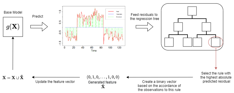
Figure 1: A visual illustration of EBLR.

The proposed method shares similar ideas with gradient boosting regression (GBR) trees. Specifically, GBR trees fit a decision tree on the residuals obtained from the fitted prediction model (or base learner) and aim to improve the prediction model by adding new decision trees to update the base prediction. At each iteration, predicted residuals are used to update the base prediction after they are multiplied with a learning rate. In other words, GBR trees use all the rules to update the prediction with a fixed learning rate. On the other hand, our approach uses the residuals to determine the highest source of errors and creates a single and interpretable feature to the fitted model to improve its predictive performance at each iteration. Compared to the use of a fixed learning rate, the base learner in the first stage is retrained to find an appropriate weight to the introduced feature. Unlike generic boosting algorithms, our method does not sacrifice interpretability while improving the prediction performance. Moreover, our method generates a fewer but more meaningful features, which leads to a more memory efficient method.

The basic time series models and other linear models rely on trends, and seasonality, and leave unexplained components as noise. Due to exponential number of potential interactions, kernel-based methods ([31]) are introduced to capture these interactions and nonlinearity without explicitly introducing the features to the model. However, these kernels cause model to lose its interpretability. The proposed approach identifies interactions between features through a regression tree in the second stage and explicitly adds this information to the model. Use of the single set of rules that contributes to the error most not only improves the predictive performance, but also allows for interpretable results. For instance, for retail sales forecasting, if there is an implicit interaction between holiday and promotion day variables that creates a higher effect than their individual effects, a new (nonlinear) variable is included in the fitted model. This variable implies that the promotion has a higher effect on the sales when applied on a holiday. In a similar manner, our approach is able to capture many polynomial interaction terms and incorporate those to the fitted model depending on the choice of the base learner (i.e. linear regression).

After generating point forecasts, the proposed model extends to probabilistic forecasting. It generates probabilistic forecasts based on the empirical error distribution which is representative of the underlying real distribution. Prediction intervals are generated by extracting quantiles through bootstrapping the residuals of the time series [16].

The rest of this paper is organized as follows. In Section 2 we provide a review of the relevant works. Section 3 introduces EBLR and its extensions with necessary backgrounds. Section 4 presents the numerical experiments and the conclusion is provided in Section 5.

2 Related Works

Time series forecasting has been well studied in the literature. While the earlier studies focused on linear statistical forecasting methods such as exponential smoothing and ARIMA, nonlinear models including neural networks has been shown to perform better for various forecasting tasks [6, 12]. Decision trees and their ensembles such as random forests and gradient boosted trees were also frequently used for time series forecasting especially due to interpretability of the model predictions [20, 36]. Recent studies particularly focused on deep learning and metalearning approaches, reporting substantial performance improvements for the time series forecasting task over the linear models as well as standard supervised learning approaches [30, 33, 35]. While these models show significant promise in generating highly accurate results especially when data is abundant, they are typically regarded as black-box models, which are not deemed as interpretable/explainable. We refer the reader to Parmezan et al. [32]’s study for a detailed overview of statistical and machine learning models for time series forecasting.

Several hybrid approaches have been considered to incorporate nonlinear relations between input and output variables. Zhang [39] assumed that each time series can be represented as a combination of linear and nonlinear components and developed a hybrid ARIMA and artificial neural network (ANN) model for forecasting. Predictions in the model were obtained as a combination of ARIMA’s forecast for the linear component and ANN’s forecast for the nonlinear component. Khashei and Bijari [26] investigated the performances of hybrid forecasting models by comparing generalized hybrid ARIMA/ANN model, Zhang [39]’s hybrid ARIMA/ANN model and ANN($p,d,q$) models. Their analysis with three different datasets showed that generalized hybrid ARIMA/ANN model, which aimed to find linear relations using ARIMA in the first stage and nonlinear relations using ANNs in the second stage, performed best among the three approaches. Aladag et al. [4] replaced the feed forward neural network in Zhang [39]’s model with a recurrent neural network (RNN), which lead to improvements in forecasting accuracy. Taskaya-Temizel and Casey [37] performed comparative analysis on ARIMA and ANN hybrids using nine different datasets, showing that components of the hybrid models outperformed their hybrid counterparts in five of the nine instances. They concluded that careful selection of the models to be combined is important for the success of the hybrid models. Arunraj and Ahrens [7] proposed a hybrid model with seasonal ARIMA (SARIMA) and quantile regression where the latter was used for forecasting the quantiles rather than individual data points. Various other studies considered hybrid models constructed from variants of ARIMA models such as SARIMA and SARIMAX [13, 14].

While the common approach for forecasting is the prediction of the expected value of a target value, understanding the uncertainty of a model’s predictions can be important in different areas such as macroeconomics and financial risk management. Accordingly, many studies on forecasting focus on modeling uncertainties that lead to probabilistic forecasts. A commonly used approach is to use quantile regression [29], while some other studies consider ensemble of learned models to generate probabilistic forecasts [3]. Recent studies focus on deep neural networks to generate mean and variance parameters of the predictive distributions. Specifically, Salinas et al. [35] propose DeepAR model, which is an autoregressive recurrent network-based global model that consider observations from different training time series to build a single probabilistic forecasting model. Rangapuram et al. [33] combine state space models with deep learning by parametrizing a linear state space model using an RNN. Wang et al. [38] integrate global deep neural network backbone with local probabilistic graphical models where global structure extracts complex nonlinear patterns and local structure captures individual random effects. Combining different probabilistic forecasting methods, Alexandrov et al. [5] provide an extensive Python library of probabilistic time series models.

Few other studies in the literature focused on building a forecasting model through residual exploration. Aburto and Weber [1] considered a combined ARIMA and neural network model where the ARIMA model was used to model the original time series and the neural network was used to predict possible forecasting errors. The resulting forecast was taken as the summation of the predicted values by these two models. Gur Ali and Pinar [22] proposed a two-stage information sharing model for multi-period retail sales forecasting problem. In their model, the first stage estimated various variables such as calendar, seasonality and promotions through a regression analysis, and second stage extrapolated the residual time series. The resulting prediction was obtained by combining the forecasts from the first stage with the extrapolated residuals from the second stage.

3 EBLR

This section introduces our framework for time-series forecasting and non-linear feature generation called Explainable Boosted Linear Regression (EBLR). Our framework consists of two stages that are applied recursively: model training and feature generation. The first stage is intuitive and utilizes well-known linear models such as linear regression, least absolute shrinkage and selection operator (LASSO) regression, or ARIMA. The second stage generates non-linear features based on regression tree transformation. Below, we first provide necessary background on the regression trees and tree-based representation, then introduce EBLR and its extensions.

3.1 Regression Trees and Tree-based Representation

Regression trees [11] are tree structures that recursively partitions the observation space based on some rules. These rules are greedily generated by evaluating all possible splits in the data and selecting the one that provides the highest mean squared-error (MSE) reduction in the children nodes.

Each terminal node in a regression tree can be represented by a set of rules. Due to the nature of the split formation in the trees, each terminal node refers to a hyperrectangle in the feature space (assuming that all features are numerical without loss of generality). From probabilistic view, regression trees model mixture of Gaussian distributions [15]. Feature representations based on the tree structures are shown to provide successful results in different domains and they are sometimes referred to as hashing [28, 40]. Similarly, each observation is represented by a binary vector based on its presence or absence in a terminal node. For instance, an observation residing in the 3$rd$ node of a regression tree with 5 terminal nodes is represented as $(0,0,1,0,0)$. This representation implicitly encodes the feature space based on the distribution of the target variable [11].

3.2 Methodology

Consider a time series dataset containing $N$ time series of length $T$. Let $y^{(i)}_{t}$ represent the observation at time $t$ of the $i^{th}$ time series and, assume that there is a $(1\times F)$ feature vector associated with each observation $y^{(i)}_{t}$, represented by $X^{(i)}_{t}$. Moreover, $\mathbf{y}$ and $\mathbf{X}$ respectively represent the vector of all observations of size ($N\times 1$) and the matrix that contains complete feature space of size ($N\times F$).

In the first phase, an initial feature set of size $f\in\{1,\dots F\}$ is selected. This feature set can contain a single feature of time information $(t)$ or a collection of features and is represented by an ($N\times f$) matrix called $\mathbf{X^{\prime}}$. Then, a linear base learner $g(\bm{x})=\alpha+\beta^{T}\bm{x}$ that maps $\mathbf{X^{\prime}}$ to a $\mathbf{\hat{y}}\in\mathbb{R}^{n}$ vector of size $(N\times 1)$ is chosen. The base learner is trained on ($\mathbf{X^{\prime}},\mathbf{y}$) pair to obtain the base model parameters $(\beta)$ by minimizing a targeted loss function. Based on the prediction vector $\mathbf{\hat{y}}$ obtained from $g(\mathbf{X^{\prime}})$, the residuals are calculated and represented as $\mathbf{e}=\mathbf{y}-\mathbf{\hat{y}}$. Note that due to the linear nature of the base learner, residuals potentially contain additional information that is related to the nonlinear patterns in the feature vectors and/or interactions.

In the second phase, the residuals obtained from the base learner are examined to model the unexplored components. Here a regression tree that predicts $\mathbf{e}$ using $\mathbf{X}$ is trained. Each observation $e_{t}^{i}\in\mathbf{e}$ resides in a single terminal node of the regression tree. Regression trees are constructed to minimize MSE of the target values that end up in each of the terminal nodes. Therefore, when they are trained on the residuals, they essentially aim to group the errors from the same sources. That is, it discovers the undiscovered, potentially nonlinear features that explains a proportion of the errors. Each terminal node in the regression tree represents an error source. Here the terminal nodes are selected such that absolute value of the target means (i.e. residuals) in the terminal nodes is the largest, i.e., terminal node with the largest error source.

The selected terminal node can be represented with a binary vector $\mathbf{\tilde{X}}\in\{0,1\}^{N}$ such that $\mathbf{\tilde{X}}_{i}=1$ if the observation $i$ resides in the selected terminal node and $0$ otherwise. Once this vector is generated, it is added to the current feature vector $\mathbf{X^{\prime}}$, which is updated by setting $\mathbf{X^{\prime}}=\mathbf{X^{\prime}}\cup\mathbf{\tilde{X}}$. This process is repeated until a stopping condition is met.

3.3 Parameters

There are three sets of parameters involved in EBLR: (1) hyperparameters of the base learner, (2) hyperparameters of the regression trees and (3) stopping condition related parameters. Firstly, hyperparameters for the selected base learner can be specified based on the prior knowledge and/or through hyperparameter tuning. Since we focus on linear models such as simple linear regression and LASSO regression, only hyperparameter that should be specified is LASSO penalty which can be easily determined by cross-validation.

Secondly, EBLR requires specification of the decision tree hyperparameters, namely, tree-depth, complexity parameter or minimum observation in terminal nodes. Determining the depth of the tree is of great importance for our method because it directly determines the degree of nonlinearity, i.e., degree of complexity, for the generated features. There are two main approaches that could be used for determining the depth: pre-pruning (determining the tree depth before construction) and post-pruning (pruning the leaf nodes after construction). For our purpose, utilization of pre-pruning is challenging since the “right amount of complexity” required for each generated feature is not known apriori to tree construction, therefore, it might need cross-validation by re-constructing the regression tree for many times which might introduce an additional complexity. Unlike pre-pruning, post-pruning based on complexity parameters provide a highly efficient pruning strategy that allows generating features of various complexities in each iteration without re-constructing the regression trees. Post-pruning requires an initial complexity parameter, $\eta$, to be specified. Our preliminary analysis show that setting $\eta$ to a small value would be enough for our method to perform well.

Lastly, the parameters are specified for the stopping criteria. In this work, the number of features to be generated $(F^{\max})$ is used as the stopping criteria which essentially implies the number of iterations that EBLR runs. It is important to note that there is a trade-off between the base model selection and stopping criteria. If the selected base model is a primitive learner such as simple linear regression, then $F^{\max}$ significantly effects the degree of over-fitting that could be faced with and it should be carefully selected. Whereas, if our base learner is a penalized method such as LASSO regression, $F^{\max}$ could be selected as a very large integer and coefficient of penalization can be tuned to eliminate the features that cause over-fitting. A pseudocode of EBLR is provided in Algorithm 1.

Input : Input Dataset $\mathcal{D}$, Number of Features $F^{\max}$, Initial Complexity Parameter $\eta$

Output : Trained model $g$

1 Construct initial feature matrix $\mathbf{X^{\prime}}$.;

2 for $i=1\ldots F^{\max}$ do

3       Train the base model g on ($\mathbf{X^{\prime}},\mathbf{y}$);

4       Calculate the residuals $\mathbf{e}=\mathbf{y}-\mathbf{\hat{y}}$ ;

5       Train a regression tree on the residuals based on $\eta$ and using all features $\mathbf{X}$ ;

6       Apply post-pruning to the regression tree.;

7       Extract a feature $\mathbf{\tilde{X}}$ from the terminal nodes with the largest absolute error ;

8       Update $\mathbf{X^{\prime}}=\mathbf{X^{\prime}}\cup\mathbf{\tilde{X}}$;

9      

10 end for

11Update feature space to include all raw features $\mathbf{X^{\prime}}=\mathbf{X^{\prime}}\cup\mathbf{X}$ ;

12 Train the base model g on ($\mathbf{X^{\prime}},\mathbf{y}$);

13 return $g$;

Algorithm 1 Pseudocode of EBLR

3.4 Complexity Analysis

We conduct a worst-case theoretical complexity analysis for EBLR. The complexity of the method is dictated by the feature generation phase due to simple and linear nature of the base regressors. We take $B$ as the complexity of the base regressor and focus on the feature generation phase.

Consider a decision tree of depth $d$ constructed on a time series database of size $N\times T$. Then, in the vertical format it corresponds to $NT$ number of observations. Since each observation requires $d$ number of comparisons, the worst-case complexity of the feature generation is $O(NTd)$. Then, the complexity of each iteration becomes $O(NTd+B)$. This process is repeated for $F^{\max}$ times, which yields $O(F^{\max}(NTd+B))$ complexity. Note that the complexity of EBLR is similar to both gradient boosting regression (GBR) and random forest (RF) which is $O(F^{\max}NTd)$ assuming $F^{\max}$ number of iterations.

3.5 Illustration

In order to provide a better understanding, we illustrate EBLR on a simple example. Consider a time series coming from the following model, initialized with $y_{0}=y_{1}=0$:

$$y_{t} =-0.4y_{t-1}+0.5y_{t-2}+5500*isWeekend*isPromotion$$

$$+1500*isPromotion+3000*isWeekend+\mathcal{N}(5000,150).$$

In this example, in addition to the auto-regressive terms, there are two factors affecting the sales: day of the week and promotion. Also, note that the interaction of these features have heterogeneous effects and are also important. For example, there is a significant difference in the effect of promotion on weekdays and weekends.

Figure 2 illustrates the predictions obtained throughout the EBLR iterations. In Figure 2a, the red line shows the original time series ($\mathbf{y}$) and the blue line represents our initial guess ($\mathbf{\hat{y}}$) which is the mean of the time series (i.e. we start with an empty feature set). Then the residuals are calculated (the difference between $\mathbf{y}$ and $\mathbf{\hat{y}}$) and a regression tree is fit to the residuals using the data with complete features ($\mathbf{X}$) presented in Figure 3. From the terminal nodes of the tree, the node with the largest mean absolute value is selected (terminal node (4)). Based on this node, a new feature ($\mathbf{\tilde{X}}$) is created such that it takes value 1 if the observation ends up in the selected terminal node and 0 otherwise. This newly generated feature corresponds to the rule of (Is Weekend, Yes) & (Is Promo, Yes). Then, this new feature is added to the feature matrix $\mathbf{X^{\prime}}$ and the base regressor is retrained. The new predictions ($\mathbf{\hat{y}}$) are illustrated with the blue line in Figure 2b. Note that some of the patterns are captured but it still is not enough to discover the underlying model.

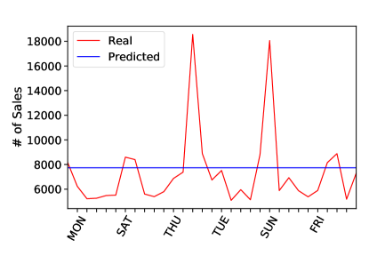
(a) Iteration 0

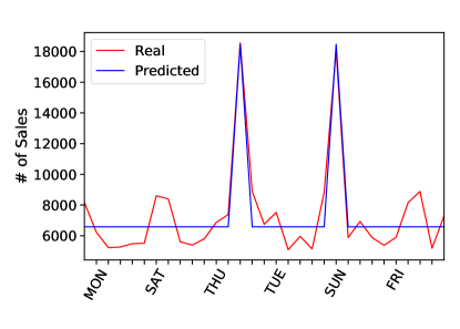
(b) Iteration 1

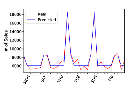
(c) Iteration 2

(d) Iteration 3

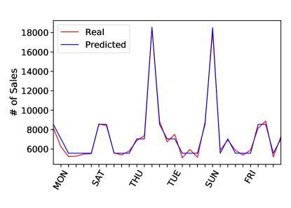
(e) Iteration 4

(f) Iteration 5

Figure 2: A sample synthetic time series and predictions of EBLR illustrating the learning process in each iteration.

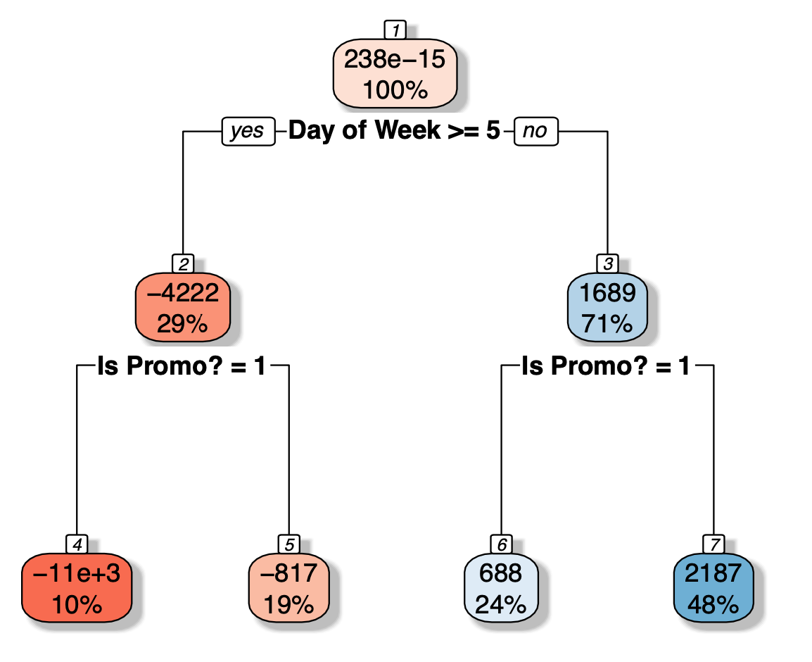
Figure 3: Regression tree trained on the residuals in the first iteration. The top and bottom values in each node respectively illustrates the mean value of the observations and the percentage of the observation falls into the node.

This feature generation and retraining phases are repeated for 5 iterations (each iteration is illustrated in Figure 2) which provides a good fit to the original time series. Another observation made here is that the early features provide major fixes in the model which are followed by minor fixes as more and more features are added to the model. This also illustrates that the selection of $F^{\max}$ parameter is important and if it is selected too large, EBLR can overfit to the data.

3.6 Feature Generation

Feature generation is an essential part of the EBLR (see Section 3.2). The features that are generated from the terminal nodes of the decision tree aim to capture the non-linear relations and interaction effects. Note that these generated features do not have any specific connection to the associated learner and can be used in other prediction models to improve their performance. From this aspect, our method can also be considered as a feature generation method.

Take a dataset of $F$ features. There are a large number of ($2^{F}-(F+1)$) interaction terms that could be considered. Also, note that each generated feature maps to a set of consecutive decision rules and the variables included in the same set of rules, represents a possible interaction between them. In addition to using these features as is, this kind of intuitive relation also allows us to consider these interaction terms in the prediction models and including them from the beginning for more complex learners.

Here, only the terminal nodes of the decision trees are explored and the node with the largest mean absolute value is selected to generate the features. However, it is possible to apply alternative approaches such as exploring all nodes rather than terminal nodes and selecting many nodes rather than only a single one in each iteration. These approaches might be more prone to over-fitting, however, it speeds-up the feature generation process.

3.7 Interpretability

Interpretability is a desired attribute for a prediction method since it brings transparency to the prediction and it increases the reliability of the algorithm. Therefore, prediction algorithms that lack interpretability might not be preferred in some applications or can create hesitancy about making a decision based on the observed results. The biggest advantage of EBLR is its ability to generate non-linear features that are also interpretable. The reason behind its interpretability is that, associated with each generated feature, there is a set of decision rules. These decision rules explicitly shows what this feature represents. Consider the first feature generated in the example provided in Section 3.5. This feature corresponds to a decision rule of {(Is Weekend, Yes) & (Is Promo, Yes)} which explicitly points out that promotion has a different effect on the weekends than weekdays. When this feature is added to the model, the corresponding coefficient shows the magnitude and direction of the effect. For example, in the example in Section 3.5, it has a positive effect which implies that promotions that are made on weekends are more effective than the weekdays.

Note that even in this simple example with two features, there are 14 possible interaction terms (7 days $\times$ 2 promo) and EBLR can easily identify that there is no difference among weekdays or weekends, and it is enough to consider whether a day is a weekday or weekend which reduces the total number of interactions to be considered to 4. With an increasing number of features in the data, identification of these interpretable features gets exponentially harder, however, EBLR can easily handle any number of features thanks to the efficient construction and interpretable structure of the decision trees.

3.8 Extension to Probabilistic Forecasting

Section 3.2 describes the proposed algorithm for forecasting a single value (mean). The algorithm can also be extended to probabilistic forecasting. This is done by constructing prediction intervals on the mean estimation based on the empirical error distributions. Assume that we are constructing a prediction interval on the $\hat{y}_{i}=g(X_{i})$, and let $E(\cdot)$ be the distribution function of the errors. Then, the $\alpha\%$ prediction interval constructed as $\hat{y}\pm E^{-1}(\alpha/100)$. This interval can be constructed for any given $\alpha$ based on the required confidence.

4 Numerical Experiments

This section provides a set of experiments to demonstrate the prediction performance of EBLR in both deterministic and stochastic settings. Before presenting the results, the experimental setup is provided. This includes the information regarding datasets, performance metrics, model settings and implementation details.

4.1 Experimental Setup

EBLR is created using both scikit-learn and r-forecast packages from two programming languages and is provided in [24]. The experiments are conducted on a 2.7 GHz dual-core i5 processor with 8GB of RAM, using the Python programming language.

4.1.1 Datasets

In this work, three datasets are utilized in the experiments: synthetic, Rossman [34] and Turkish electricity. Summary information regarding these datasets can be found in Table 1.

Table 1: Descriptive information and statistics on the datasets.

	Synthetic	Rossmann	Turkish Electricity
# features	1	6	2
# time covariates	1	53	31
# time series	1	100	1
# avg data points / time series	2048	918.1	8760
Granularity	Daily	Daily	Hourly
Seasonality	None	None	Daily
Forecast Horizon	14 days	28 days	14 hours
# of tests	25	100	25

Synthetic dataset. The first dataset is a synthetically generated dataset that mimics a simple version of daily sales of a retail store. Figure 4 demonstrates a sample from this synthetic dataset. Note that the same approach is used in Section 3.5 for illustration purposes.

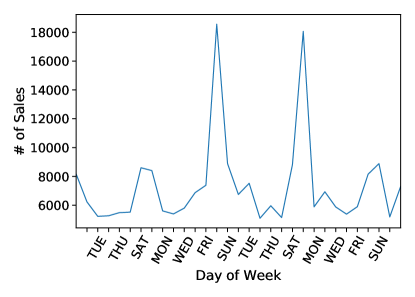
Figure 4: A one-month training snapshot of the synthetic dataset, showcasing linear features (small peaks) and two non-linear interactions (large peaks).

Rossman dataset. The Rossmann sales data is a feature-rich dataset, containing features related to the date, number of customers, holiday-specific information, promotional information, and store closures. The sales of an individual store is set to the target variable, and the customer covariate was removed because it is related to the target variable, and requires to be forecasted. The date feature is further decomposed into the day of the week, day of the month, month of the year, and year features for enriching the feature space.

Turkish electricity dataset. Finally, the highly seasonal Turkish electricity consumption dataset is used. Here, the prediction focus is on the electricity consumption of Turkey’s most populated city’s (Istanbul). This target variable is created by interpolating the total electricity consumption in Turkey to Istanbul (based on monthly factors). This dataset is decomposed into hourly consumption rates, with daily seasonality. Then, the date is decomposed into the day of the week, month and year variables. Moreover, the data contains daily high and low temperatures of Istanbul which is an important determinant of electricity consumption.

4.1.2 Performance Metrics

In this work, three performance metrics are considered similar to [35]. Point forecasting performance is compared in terms of the normalized root mean squared error (NRMSE) and the normalized deviation (ND). Explicit expressions for the metrics are provided as follows:

$$\text{NRMSE}(y,\hat{y}) =\frac{\sqrt{\frac{1}{N}\sum_{i=1}^{N}(\hat{y_{i}}-y_{i})^{2}}}{\frac{1}{N}\sum_{i=1}^{N}|y_{i}|}$$ (1)

$$\text{ND}(y,\hat{y}) =\frac{\sum_{i=1}^{N}|\hat{y_{i}}-y_{i}|}{\sum_{i=1}^{N}|y_{i}|}$$ (2)

For the probabilistic forecasting, the models are evaluated on the weighted scaled pinball loss at the 0.05, 0.25, 0.50, 0.75 and 0.95 quantiles. To combine these five metrics into one general metric, the mean of the quantile losses is also reported. For any quantile $\rho$, the weighted scaled pinball loss is calculated as follows:

$$\text{WSPL}_{\rho}(y,\hat{y}^{\rho}) =\frac{\sum_{i=1}^{N}\max\{\rho(y_{i}-\hat{y_{i}}^{\rho}),(1-\rho)(\hat{y_{i}}^{\rho}-y_{i})\}}{\sum_{i=1}^{N}|y_{i}|}$$ (3)

4.1.3 Model Settings

In the point forecasting experiments, EBLR is compared against two naive methods: linear regression (LR) and a baseline method (Mean), statistical models: ARIMAX, and ensemble methods: gradient boosting regressor (GBR) [18], random forest regressor (RF) [10]. LASSO penalty is selected based on 5-fold cross-validation. For ARIMA based models (e.g. ARIMAX), a step-wise algorithm is used to tune the model (see  [23] for details). In the case of the seasonal Turkish electricity dataset, the seasonal parameters are included in the ARIMAX model as well. This is because the Turkish electricity dataset is inherently seasonal [25]. For GBR and RF, a single parameter setting is utilized without performing hyperparameter tuning, and this setting is used consistently across all datasets. The parameters for GBR and RF can be found in Table 2.

Table 2: The hyperparameter setting used in the experiments for gradient boosting regression (GBR) and random forest (RF).

	GBR	RF
# of trees	100	100
Splitting Criterion	Friedman MSE	MSE
Max Depth	3	$\infty$
Loss Function	Least Squares Regression	N/A
Learning Rate	0.1	N/A

Moreover, for EBLR, the parameter setting for each dataset are specified in Table 3. Only a small number of parameters were selected in the synthetic data set since it was known that there were only a few underlying features. Then, 50 features were arbitrarily chosen to be learned in the Rossmann data set. When this setting was reused on the Turkish dataset, it was found that the model was still learning, therefore the number of features was doubled. All the initial complexity parameters where chosen such that they were significantly small.

Table 3: EBLR parameters used in the experiments for three datasets.

	Synthetic	Rossmann	Turkish Electricity
# of features	5	50	100
Initial Complexity Parameter	0.001	0.001	0.001

In all the probabilistic forecasting experiments, EBLR was compared against both ensemble methods as found in point forecasting. In order to generate probabilistic results, the loss function was adjusted in the gradient boosted regressor model to use quantile loss, and a model was trained for each quantile. In addition, in random forest, the quantiles were collected based on the individual regressors. The other models use a more naive forecasting approach, by training prediction intervals based on the training residuals. All the experiments were repeated with the same feature setups, however, instead the 5%, 25%, 50%, 75% and 95% quantile predictions were collected. As expected, it is seen that all of the 50% quantiles perform similarly to the ND scores.

4.2 Improvement over Base Regressors

This section presents an experiment on EBLR’s contribution on improving the prediction performances of linear regression, LASSO regression and ARIMA methods. Table 4 illustrates the average forecasting performances of these methods with and without EBLR on synthetic dataset and Rossmann dataset. From these results, it can observed that utilizing EBLR provides significant decrease in the NRMSE and ND for both linear regression, LASSO and ARIMA methods, especially for the synthetic dataset. Note that since these base regressors are linear, they fail to capture the interaction effect in the synthetic data whereas incorporating these base regressors in EBLR allows the generation of interaction features which reduces the error significantly. Since EBLR provides similar results with all base regressors, we utilize LASSO regression as the base regression in the future experiments with the aim of preventing potential over-fitting.

Table 4: Point forecasting results for linear regression, LASSO regression and ARIMA methods with their EBLR version.

		Linear Regression		LASSO		ARIMA
		w/o EBLR	w EBLR	w/o EBLR	w EBLR	w/o EBLR	w EBLR
Synthetic	NRMSE	0.3265	0.0471	0.3264	0.0472	0.3383	0.0471
	ND	0.2474	0.0383	0.2473	0.0384	0.2626	0.0383
Rossmann	NRMSE	0.1731	0.1528	0.1750	0.1543	0.1754	0.1613
	ND	0.1252	0.1085	0.1270	0.1088	0.1284	0.1164

4.3 Point Forecasting

The prediction performances over three datasets are provided in Table 5, moreover, Figure 5 illustrates the predictions of four important regressors on single time series from each of these three datasets. The first set of experiments are run on a synthetic data set and the results are presented in the second and third columns of Table 5. From these results, three specific observations can be made: (1) EBLR significantly improves the performance of linear regression (decrease NRMSE from 0.3265 to 0.0472) by introducing 5 additional features that captures the important interactions. (2) EBLR outperforms all primitive regression algorithms including ARIMAX, linear regression and naive baseline. (3) EBLR provides comparable performances to the ensemble methods.

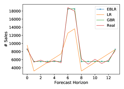
(a) Synthetic dataset

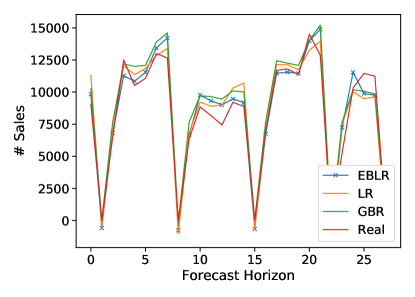
(b) Rossmann

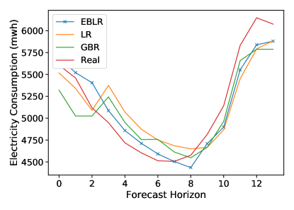
(c) Turkish electricity

Figure 5: Three different point forecasting tests of EBLR, linear regression (LR), gradient boosting regressor (GBR). The order (from left to right, top to bottom) include a 14 period forecast with respective predictions, a 28 period sales forecast, and a 14 hour electricity consumption forecast.

Secondly, we focus on the Rossmann dataset where the results are presented in the fourth and fifth columns of Table 5. In the Rossmann dataset, EBLR performs slightly worse than GBR, but once again outperforms ARIMAX, linear regression and naive baseline models. When EBLR is compared to random forest, a more interesting relationship is revealed. EBLR has a lower NRMSE whereas random forest has a lower ND. This means that EBLRs predictions tend to be more consistent, whereas random forest on average makes a more accurate prediction, however the poor predictions are much worse than EBLRs. Finally, the last two columns of Table 5 demonstrates the results on Turkish electricity dataset, where, consistent with the previous datasets, EBLR outperforms ARIMAX, linear regression, and naive baseline models. In addition, EBLR also outperforms GBR, but not RF.

Overall, EBLR provides substantial improvement to the linear regression by incorporating additional features. Moreover, even though EBLR is completely interpretable, it provides comparative performance to the state-of-the-art ensemble-based methods.

Table 5: Point forecasting results over all three datasets for EBLR, random forest (RF), gradient boosting regression (GBR), ARIMAX, linear regression and naive baseline methods.

Model	Synthetic		Rossmann		Turkish Electricity
	NRMSE	ND	NRMSE	ND	NRMSE	ND
EBLR	0.0472	0.0384	0.1528	0.1085	0.0428	0.0348
RF	0.0471	0.0384	0.1670	0.1017	0.0297	0.0234
GBR	0.0471	0.0384	0.1507	0.0986	0.0581	0.0466
ARIMAX	0.3384	0.2626	0.1754	0.1284	0.0500	0.0297
Linear Regression	0.3265	0.2474	0.1750	0.1270	0.0530	0.0424
Baseline	0.4778	0.3007	0.5880	0.4155	0.1171	0.1019

4.4 Probabilistic Forecasting

This section presents probabilistic forecasting results on the three datasets. The first set of results focus on the synthetic dataset for which the summary statistics are presented in Table 6, and example probabilistic forecasts for EBLR, GBR and ARIMAX models are provided in Figure 6. Overall, EBLR performs the same as GBR and outperforms all other competitors. EBLR captures the tails very well as well as the median predictions. This suggests that EBLR extends to probabilistic forecasting successfully.

Table 6: Synthetic probabilistic forecasting results for the five specified quantiles and their combined mean for EBLR, random forest (RF), gradient boosting regression (GBR), ARIMAX, linear regression and naive baseline methods.

Model	WSPL($\rho$)
	0.05	0.25	0.50	0.75	0.95	Mean
EBLR	0.0051	0.0157	0.0192	0.0153	0.0048	0.0120
GBR	0.0053	0.0156	0.0192	0.0152	0.0048	0.0120
RF	0.0168	0.0186	0.0192	0.0187	0.0169	0.0180
MEAN	0.0397	0.0848	0.1504	0.1829	0.0976	0.1111
ARIMAX	0.0337	0.0986	0.1246	0.1175	0.0473	0.0843

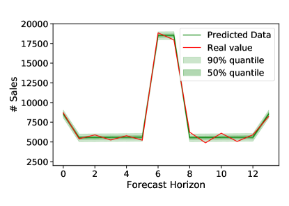
(a) EBLR

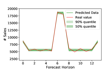
(b) GBR

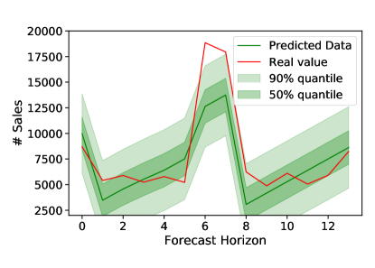
(c) ARIMAX

Figure 6: Three different probabilistic forecasting interval results on a sample forecasting horizon. Each forecast horizon contains the median forecast (dark green line), the 50% forecast interval (medium green fill), and 90% forecast interval (light green fill).

Secondly, the performances of the subjected methods are evaluated on the Rossmann dataset. Table 7 illustrates the performances of the considered methods and Figure 7 provides an illustration of the predictions for EBLR, GBR and ARIMAX methods. Here, EBLR performs worse than GBR, however, it outperforms all other methods. One important observation is that the relative performance of EBLR to GBR is better in extreme quantiles. This indicates that EBLR accounts for unlikely outcomes more than GBR.

Table 7: Three different probabilistic forecasting interval on a sample Rossmann store 28 day forecast. Each forecast horizon contains the median forecast (dark green line), the 50% forecast interval (medium green fill), and 90% forecast interval (light green fill).

Model	WSPL($\rho$)
	0.05	0.25	0.50	0.75	0.95	average
EBLR	0.0185	0.0466	0.0539	0.0409	0.0140	0.0348
GBR	0.0161	0.0401	0.0474	0.0376	0.0162	0.0315
RF	0.0226	0.0421	0.0527	0.0429	0.0144	0.0349
MEAN	0.0626	0.2032	0.2078	0.1575	0.0556	0.1373
ARIMAX	0.0195	0.0538	0.0627	0.0506	0.0182	0.0410

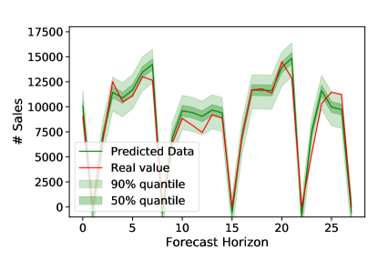
(a) EBLR

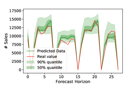
(b) GBR

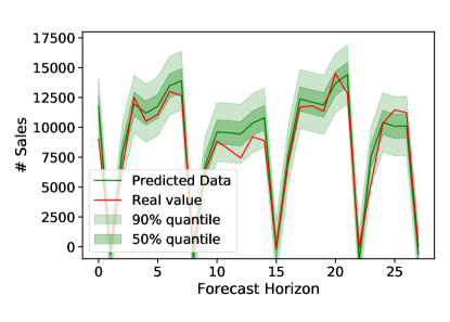
(c) ARIMAX

Figure 7: Three different probabilistic forecasting interval results on a 28 day forecast horizon for a selected Rossmann store. Each forecast horizon contains the median forecast (dark green line), the 50% forecast interval (medium green fill), and 90% forecast interval (light green fill).

Lastly, Table 8 and Figure 11 respectively illustrate the experiment results and example predictions of different methods for the Turkish electricity dataset. From these results, in contrast to the Rossman dataset, EBLR outperforms GBR at all quantiles. This could be attributed to GBR overfitting the data set and starting to include noise from training data into the model. EBLR is able to outperform the baseline model as well as outperforming the ARIMAX model. A unique observation is that, since the ARIMAX model is given extra seasonal regressors in this example, it is able to properly formulate the auto-regressive nature of electricity consumption. On the other hand, EBLR is able to incorporate this seasonality without having these explicit auto-regressive features.

Table 8: Three different probabilistic forecasting interval on a 14 hour Istanbul total electricity consumption. Each forecast horizon contains the median forecast (dark green line), the 50% forecast interval (medium green fill), and 90% forecast interval (light green fill).

Model	WSPL($\rho$)
	0.05	0.25	0.50	0.75	0.95	Mean
EBLR	0.0049	0.0149	0.0177	0.0130	0.0035	0.0108
GBR	0.0089	0.0211	0.0226	0.0179	0.0079	0.0157
RF	0.0036	0.0089	0.0105	0.0089	0.0039	0.0072
Mean	0.0123	0.0395	0.0509	0.0353	0.0120	0.0300
ARIMAX	0.0075	0.0158	0.0148	0.0131	0.0055	0.0113

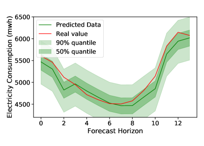
(a) EBLR

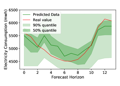
(b) GBR

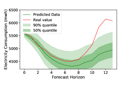
(c) ARIMAX

Figure 8: Three different probabilistic forecasting interval results on a 14 hour electricity forecast horizon for electricity consumption in Istanbul. Each forecast horizon contains the median forecast (dark green line), the 50% forecast interval (medium green fill), and 90% forecast interval (light green fill).

For posterity, EBLR was compared to a DeepAR model consisting of two LSTM layers of 40 cells each [35]. The comparison is realized on the Rossman dataset since deep learning methods require very large number of instances to properly function [35]. Although it has a highly complex structure, DeepAR produces an NRMSE of 0.1495 which is only a marginal improvement over EBLR. In terms of probabilistic forecasts, the average WSPL across the considered quantiles for DeepAR is 0.0320. This result is worse than GBR’s average WSPL, and marginally better than EBLRs. As well, all this overhead comes at the cost of interpretability since DeepAR is regarded as a black-box model.

4.5 Model Interpretability

This section focuses on the explainability by illustrating the interpretable nonlinear features generated by EBLR for these datasets. It is illustrated in Section 3.5 that EBLR is capable of discovering the interaction effects. For example, in the process of learning the underlying model of the synthetic data set, the following features are learned:

1. Is the day a weekend with a promotion?

2. Is the day a weekend without a promotion?

3. Is the day a weekday with a promotion

4. Is the day a weekday without a promotion?

This aligns with the synthesized features. First, EBLR learns how weekends deal with promotions, and then it determines how weekdays deal with promotions. This can clearly be seen in Figure 2, where the strong weekend features are learned then the weekday features are learned. As well, after these four features are learned, the model is terminated since the regression tree can not find a split.

Similarly, in the Rossmann data set a key learned feature is if the date is a Monday, without any promotions, and no school holiday. This feature contributes negatively to the prediction which is intuitive to understand. People typically do not shop on Mondays unless there is a special event. Other contributing features are tied relations between the month of the year, promotional activity, and school holidays. This is easily extracted through EBLR, which provides valuable data insights.

The progression of EBLR’s learning process can be seen through plotting the NRMSE against the number of features. A sample learning curve has been plotted for a particular Rossman store in Figure 9.

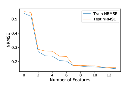
Figure 9: EBLR’s improvement in NRMSE for a sample Rossmann sales store, as more features are generated and added to the base linear learner.

Feature importance scores are generated based on these rules, combined with the learning curve. For each rule that is created, there is a change in the residual error, $\Delta e$. Earlier learned features decrease the residual error tremendously, whereas fine-tuning features are deemed not as important. This error is allocated to all boolean decisions in the feature. For example, when EBLR first learns the feature (Is Weekend, Yes), ${\Delta e_{1}}$ is assigned to each feature for $isWeekend$ and $isPromo$. This is done for each feature generated, and then all the scores are added together and normalized. For example, in the synthetic dataset in Section 3.5, every feature generated consists of a combination of $isPromotion$ and $isWeekend$. Since these features exist in all the rules, as well as the only features that EBLR utilizes, they both receive an equal feature importance score of 0.5.

In Figure 9, there are initially a few features that drastically improve the model. Then, the model learns more complex non-linear features to continue learning. At each iteration, there is a change in how the underlying baseline linear model performs. By utilizing the proposed feature importance scoring technique, the most contributing features in the generated rules are extracted. A plot of the feature importance scores of the top 10 most important features in the Rossmann dataset in Figure 10.

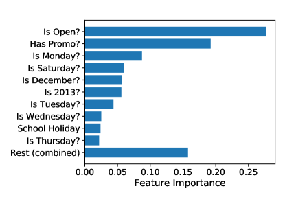
Figure 10: The top 10 important features in all of the Rossmann stores, organized from most important to least. They are equally weighted across all stores to generate all feature importance’s in the Rossmann dataset.

For the Turkish electricity data set, there is a wider spread of feature importance as observed in Figure 11b. The two most important features are the daily high and lower temperatures, followed by information about the hour of the day and if the day was a Sunday. Together, these feature importance scores imply that electricity usage is highly dependent on temperature and the hour of the day. EBLR cares about knowing if the day is a Sunday or not, which means Sundays behave differently than the remaining days of the week. As well, there is an even distribution of feature usage in the Turkish electricity dataset, compared to a few key features in the Rossmann dataset.

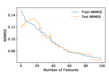
(a) Sample Learning Curve

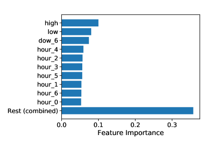
(b) Top 10 Feature Importance

Figure 11: (Left) The NRMSE learning curve compared to the number of features in a the Turkish electricity dataset. (Right) The top 10 most importance features in the Turkish electricity consumption dataset, organized from most important to least.

5 Conclusion

Through the probabilistic and point forecasting experimentation, it is evident that EBLR is a strong boosting algorithm. While there was no clear separation between the EBLR, GBR, and RF, it is clear that EBLR is much simpler than the other two ensemble methods. EBLR consists of simple binary features, compared to the complexity of storing numerous decision trees. On top of this, the information lost by only storing these relevant binary features is minimal.

EBLR generates simple binary features through a two-step process. First, a simple baseline model is fit to a training dataset. The residuals are extracted and passed into a feature generating decision tree. This decision tree extracts the largest source of error in the form of an interpretable feature which is passed back into the baseline learner. This process is repeated until a stopping condition is met. By learning in this manner, EBLR has inherent interpretability baked into itself.

To extend EBLR to generate probabilistic forecasts, an empirical distribution is generated from EBLR’s training residuals. Quantiles are selected from this distribution, and used in making prediction intervals. While this was able to yield strong results in the three provided experiments, future work should focus on different ways to generate these prediction intervals. By generating prediction intervals in this manner, there are constant prediction intervals across all points. In reality, some specific points are more difficult to predict than others. Some potential research paths include using a quantile base linear learner or extracting more information from the feature generating decision trees.

References

- Aburto and Weber [2007] Aburto, L., Weber, R., 2007. Improved supply chain management based on hybrid demand forecasts. Applied Soft Computing 7, 136–144.
- Adadi and Berrada [2018] Adadi, A., Berrada, M., 2018. Peeking inside the black-box: A survey on explainable artificial intelligence (xai). IEEE Access 6, 52138–52160.
- Ahmed Mohammed and Aung [2016] Ahmed Mohammed, A., Aung, Z., 2016. Ensemble learning approach for probabilistic forecasting of solar power generation. Energies 9, 1017.
- Aladag et al. [2009] Aladag, C.H., Egrioglu, E., Kadilar, C., 2009. Forecasting nonlinear time series with a hybrid methodology. Applied Mathematics Letters 22, 1467–1470.
- Alexandrov et al. [2019] Alexandrov, A., Benidis, K., Bohlke-Schneider, M., Flunkert, V., Gasthaus, J., Januschowski, T., Maddix, D.C., Rangapuram, S., Salinas, D., Schulz, J., et al., 2019. Gluonts: Probabilistic time series models in python. arXiv preprint arXiv:1906.05264 .
- Alon et al. [2001] Alon, I., Qi, M., Sadowski, R.J., 2001. Forecasting aggregate retail sales: A comparison of artificial neural networks and traditional methods. Journal of Retailing and Consumer Services 8, 147–156.
- Arunraj and Ahrens [2015] Arunraj, N.S., Ahrens, D., 2015. A hybrid seasonal autoregressive integrated moving average and quantile regression for daily food sales forecasting. International Journal of Production Economics 170, 321–335.
- Baboo and Shereef [2010] Baboo, S.S., Shereef, I.K., 2010. An efficient weather forecasting system using artificial neural network. International Journal of Environmental Science and Development 1, 321.
- Box et al. [2015] Box, G.E., Jenkins, G.M., Reinsel, G.C., Ljung, G.M., 2015. Time series analysis: forecasting and control. John Wiley & Sons.
- Breiman [2001] Breiman, L., 2001. Random forests. Machine Learning 45, 5–32.
- Breiman et al. [1984] Breiman, L., Friedman, J., Stone, C.J., Olshen, R.A., 1984. Classification and regression trees. CRC press.
- Chu and Zhang [2003] Chu, C.W., Zhang, G.P., 2003. A comparative study of linear and nonlinear models for aggregate retail sales forecasting. International Journal of Production Economics 86, 217–231.
- Cools et al. [2009] Cools, M., Moons, E., Wets, G., 2009. Investigating the variability in daily traffic counts through use of arimax and sarimax models: Assessing the effect of holidays on two site locations. Transportation Research Record 2136, 57–66.
- Cornelsen and Normand [2012] Cornelsen, L., Normand, C., 2012. Impact of the smoking ban on the volume of bar sales in ireland: Evidence from time series analysis. Health Economics 21, 551–561.
- Criminisi et al. [2012] Criminisi, A., Shotton, J., Konukoglu, E., 2012. Decision forests: A unified framework for classification, regression, density estimation, manifold learning and semi-supervised learning. Foundations and Trends in Computer Graphics and Vision 7, 81–227. doi:10.1561/0600000035.
- Davison and Hinkley [1997] Davison, A.C., Hinkley, D.V., 1997. Bootstrap methods and their application. 1, Cambridge university press.
- Deb et al. [2017] Deb, C., Zhang, F., Yang, J., Lee, S.E., Shah, K.W., 2017. A review on time series forecasting techniques for building energy consumption. Renewable and Sustainable Energy Reviews 74, 902–924.
- Friedman [2001] Friedman, J.H., 2001. Greedy function approximation: a gradient boosting machine. Annals of statistics , 1189–1232.
- Friedman et al. [2008] Friedman, J.H., Popescu, B.E., et al., 2008. Predictive learning via rule ensembles. The Annals of Applied Statistics 2, 916–954.
- Galicia et al. [2019] Galicia, A., Talavera-Llames, R., Troncoso, A., Koprinska, I., Martínez-Álvarez, F., 2019. Multi-step forecasting for big data time series based on ensemble learning. Knowledge-Based Systems 163, 830–841.
- Guidotti et al. [2018] Guidotti, R., Monreale, A., Ruggieri, S., Turini, F., Giannotti, F., Pedreschi, D., 2018. A survey of methods for explaining black box models. ACM Computing Surveys (CSUR) 51, 1–42.
- Gur Ali and Pinar [2016] Gur Ali, O., Pinar, E., 2016. Multi-period-ahead forecasting with residual extrapolation and information sharing—utilizing a multitude of retail series. International Journal of Forecasting 32, 502–517.
- Hyndman et al. [2007] Hyndman, R.J., Khandakar, Y., et al., 2007. Automatic time series for forecasting: The forecast package for R. 6/07, Monash University, Department of Econometrics and Business Statistics.
- Ilic et al. [2020a] Ilic, I., Gorgulu, B., Cevik, M., 2020a. https://github.com/irogi.
- Ilic et al. [2020b] Ilic, I., Gorgulu, B., Cevik, M., 2020b. Augmented out-of-sample comparison method for time series forecasting techniques, in: Canadian Conference on Artificial Intelligence, Springer. pp. 302–308.
- Khashei and Bijari [2012] Khashei, M., Bijari, M., 2012. Which methodology is better for combining linear and nonlinear models for time series forecasting? Journal of Industrial and Systems Engineering .
- Krollner et al. [2010] Krollner, B., Vanstone, B.J., Finnie, G.R., 2010. Financial time series forecasting with machine learning techniques: A survey., in: Esann.
- Lin et al. [2014] Lin, G., Shen, C., Shi, Q., Van den Hengel, A., Suter, D., 2014. Fast supervised hashing with decision trees for high-dimensional data, in: Proceedings of the IEEE Conference on Computer Vision and Pattern Recognition, pp. 1963–1970.
- Liu et al. [2015] Liu, B., Nowotarski, J., Hong, T., Weron, R., 2015. Probabilistic load forecasting via quantile regression averaging on sister forecasts. IEEE Transactions on Smart Grid 8, 730–737.
- Ma and Fildes [2020] Ma, S., Fildes, R., 2020. Retail sales forecasting with meta-learning. European Journal of Operational Research .
- Müller et al. [1997] Müller, K.R., Smola, A.J., Rätsch, G., Schölkopf, B., Kohlmorgen, J., Vapnik, V., 1997. Predicting time series with support vector machines, in: International Conference on Artificial Neural Networks, Springer. pp. 999–1004.
- Parmezan et al. [2019] Parmezan, A.R.S., Souza, V.M., Batista, G.E., 2019. Evaluation of statistical and machine learning models for time series prediction: Identifying the state-of-the-art and the best conditions for the use of each model. Information Sciences 484, 302–337.
- Rangapuram et al. [2018] Rangapuram, S.S., Seeger, M.W., Gasthaus, J., Stella, L., Wang, Y., Januschowski, T., 2018. Deep state space models for time series forecasting, in: Advances in Neural Information Processing Systems, pp. 7785–7794.
- [34] Rossmann Store Sales, 2020. URL: https://www.kaggle.com/c/rossmann-store-sales.
- Salinas et al. [2020] Salinas, D., Flunkert, V., Gasthaus, J., Januschowski, T., 2020. Deepar: Probabilistic forecasting with autoregressive recurrent networks. International Journal of Forecasting 36, 1181–1191.
- Taieb and Hyndman [2014] Taieb, S.B., Hyndman, R.J., 2014. A gradient boosting approach to the kaggle load forecasting competition. International Journal of Forecasting 30, 382–394.
- Taskaya-Temizel and Casey [2005] Taskaya-Temizel, T., Casey, M.C., 2005. A comparative study of autoregressive neural network hybrids. Neural Networks 18, 781–789.
- Wang et al. [2019] Wang, Y., Smola, A., Maddix, D.C., Gasthaus, J., Foster, D., Januschowski, T., 2019. Deep factors for forecasting. arXiv preprint arXiv:1905.12417 .
- Zhang [2003] Zhang, G.P., 2003. Time series forecasting using a hybrid arima and neural network model. Neurocomputing 50, 159–175.
- Zhou et al. [2019] Zhou, M., Zeng, X., Chen, A., 2019. Deep forest hashing for image retrieval. Pattern Recognition 95, 114–127.