Street Network Models and Indicators for Every Urban Area in the World

Abstract

Cities worldwide exhibit a variety of street network patterns and configurations that shape human mobility, equity, health, and livelihoods. This study models and analyzes the street networks of every urban area in the world, using boundaries derived from the Global Human Settlement Layer. Street network data are acquired and modeled from OpenStreetMap with the open-source OSMnx software. In total, this study models over 160 million OpenStreetMap street network nodes and over 320 million edges across 8,914 urban areas in 178 countries, and attaches elevation and grade data. This article presents the study’s reproducible computational workflow, introduces two new open data repositories of ready-to-use global street network models and calculated indicators, and discusses summary findings on street network form worldwide. It makes four contributions. First, it reports the methodological advances of this open-source workflow. Second, it produces an open data repository containing street network models for each urban area. Third, it analyzes these models to produce an open data repository containing street network form indicators for each urban area. No such global urban street network indicator dataset has previously existed. Fourth, it presents a summary analysis of urban street network form, reporting the first such worldwide results in the literature.

1. Introduction

Street networks shape the city. They structure the circulation patterns of people and goods and underlie urban accessibility. Differences in street network geometry and topology—collectively, “form”—worldwide reflect different cultures, political systems, urbanization eras, technology, design paradigms, climates, and terrain. These networks in turn organize physical urban space and influence the ability to traverse it via different modes of transportation.

Yet in this era of post-globalization, little is known about comparative street network form worldwide at the urban scale. This is largely due to data access and computational limitations. Traditionally, delineating consistent urban area boundaries was difficult, making it challenging to define consistent study sites (Lemoine-Rodríguez et al.,, 2020). Even if consistent study sites could be established, it was nearly impossible to gather consistent comprehensive street network data around the world. And even if one did, it was nearly impossible to manipulate and organize the hundreds of millions of geospatial elements that that would entail, then model them in a graph-theoretic way, then compute geometric and topological indicators of form. Nevertheless, such models, indicators, and analyses would be useful for understanding urbanization patterns, transportation infrastructure planning, and the path to sustainable urban form for cities worldwide.

This study takes advantage of several emerging tools, technologies, and open data to model the individual street networks of every urban area in the world, compute geometric and topological indicators, and analyze them. It uses the Global Human Settlement Layer (GHSL) to define urban area boundaries and other variables. Using OSMnx, it downloads and models urban-scale street network data globally from OpenStreetMap, attaches elevation data, then calculates indicators for each urban area. It places all of the resulting network models, indicators, and code into open data repositories for public reuse.

This article reports the novel methods employed in this modeling and analytics project. Then it documents the street network model repository and its contents and the indicators repository and its contents. Next it presents a high-level analysis of worldwide urban street network form, using these models and indicators. Across all urban areas worldwide, both total street length and intersection count scale sublinearly with population. Higher per capita GDP is associated with higher per capita total street length. Validation reveals that the open data used as elevation attributes compare favorably with high-quality commercial data. The article concludes with notes on reuse. In sum, this study produces the first comprehensive public data repository of ready-to-use urban street network models and indicators worldwide and reports the first such worldwide analytical results.

2. Background

2.1. Street Network Models

Street network models come in many flavors, but most commonly are mathematical models called graphs (Newman,, 2003, 2010; Trudeau,, 1994; Vespignani,, 2018; Brandes and Erlebach,, 2005; Gastner and Newman,, 2006). Graphs can represent both the geometry and the topology of a real-world street network. Abstractly, a graph $G$ comprises a set of nodes (i.e., elements) $N$ which are linked to one another by a set of edges (i.e., connections) $E$. Each edge $e$ in set $E$ either connects two nodes or connects a single node to itself as a self-loop. Parallel edges exist when multiple edges connect the same two nodes.

Network modelers must decide on several theoretical aspects of representation, including directedness, planarity, and primality (O’Sullivan,, 2014; Marshall et al.,, 2018). In the case of a directed graph, all the edges in $E$ point one-way from some node $u$ to another node $v$. This may allow for the possibility of a self-loop where $u=v$. In the case of an undirected graph, all the edges in $E$ point bidirectionally between the nodes they link. If a graph is planar, all the edges in $E$ intersect in a two-dimensional plane exclusively at nodes in $N$. If this condition does not hold, the graph is nonplanar (Cardillo et al.,, 2006; Hopcroft and Tarjan,, 1974; Masucci et al.,, 2009; Székely,, 2004; Viana et al.,, 2013). A primal graph of a street network models intersections and dead-ends as nodes and the street segments that connect them as edges (Porta et al., 2006b, ). A dual graph of a street network does the opposite, modeling street segments as nodes and intersections as edges (Porta et al., 2006a, ). Real-world street networks often have self-loops, parallel edges, flow directionality restrictions such as one-way streets, and nonplanar elements such as overpasses and underpasses (Boeing,, 2017).

2.2. Street Network Data

Data on street networks around the world exist in various sources of various quality and accessibility. Many are digitized by local or regional authorities, resulting in inconsistencies in digitization standards, spatial validity, attribute data quality, and file formatting. High-quality street network geometry data exist for most developed countries, but data inconsistencies and language barriers make international cross-sectional comparison difficult. Furthermore, most such datasets exist in shapefile format and thus contain network geometry but minimal information about topology. Yet both geometry and topology are essential to consider in most spatial network analyses. Street networks are spatially embedded and are thus defined by both their geometry (e.g., positions, lengths, areas, angles, etc.) and their topology (i.e., connections and configurations) (Barthelemy,, 2011; O’Sullivan,, 2014).

Given these limitations, better data sources and network models are important for international street network analysis. Four key areas of improvement would include: 1) global coverage and availability, 2) consistent digitization and attribute data, 3) consistent representation of both geometric and topological data, and 4) better public accessibility and usability. Online geographic information systems, volunteered geographic information, and crowd-sourced big data create new opportunities to address these points. In particular, OpenStreetMap offers an important alternative source of street network data (Jokar Arsanjani et al.,, 2015).

OpenStreetMap is an open-source, collaborative, worldwide mapping project and database. One can query its database for street and intersection data, along with attribute data about road types, names, and (when available) speeds, widths, and numbers of lanes. It offers good global coverage and high geometric and topological data quality (Girres and Touya,, 2010; Haklay,, 2010; Corcoran et al.,, 2013; Zielstra et al.,, 2013; Barron et al.,, 2014; Maier,, 2014; Basiri et al.,, 2016; Sehra et al.,, 2020). Barrington-Leigh and Millard-Ball, (2017) found that, as of 2016, OpenStreetMap was 83% complete worldwide, over 40% of countries’ (including many developing countries) street networks were effectively 100% complete, and completeness was highest in both dense cities and sparsely populated areas.

As of 2021, OpenStreetMap has more than 7 million contributors who have added over 6.6 billion nodes (points), 730 million ways (lines and boundaries), and attendant attribute data to its database. Volunteers provide editorial oversight of contributions and changes. However, despite its large user base, researchers estimate that >95% of these contributors are male, and as such, there may be correlated biases in the contributed content (Schmidt and Klettner,, 2013; Graham et al.,, 2015). While OpenStreetMap road coverage is generally good worldwide, other geospatial features have better coverage in developed countries and in cities versus small towns. No data source is perfect, but OpenStreetMap is global, publicly-accessible, free, and an Open Source Initiative affiliate.

Accordingly, OpenStreetMap helps address the first three of the four areas of improvement listed earlier. However, the fourth problem persists: it is not particularly accessible or usable for less-technical urban scholars to use its data for graph models and analytics. Researchers usually acquire OpenStreetMap data through its APIs or by downloading a prepackaged data extract from a third-party. Either option offers useful raw data but usually requires writing and testing hundreds of lines of code to process topological relations and construct graph models. Doing this on an ad hoc basis introduces challenges for interpretation and replication as many small computational and modeling decisions get made along the way, such as the exact handling of common street network features like self-loops, parallel edges, and culs-de-sac. A consistent set of well-documented models and indicators, generated with an accessible open-source workflow, would improve what is otherwise often a black box (Boeing, 2020b, ).

2.3. Street Network Indicators

Several efforts in recent years have aimed to address these challenges and generate sets of urban street network indicators. For example, the OSMnx project takes this motivation to develop an open-source Python package for automatically downloading, modeling, and analyzing street networks and other geospatial features from OpenStreetMap (Boeing,, 2017). Using this tool, a recent project modeled the street networks of every US city/town, county, urbanized area, census tract, and Zillow-defined neighborhood, placed these models online in a public open data repository, and conducted spatial network analyses on them (Boeing, 2020a, ).

Similarly, Dingil et al., (2018) used OSMnx to calculate transportation indicators for 151 urban areas worldwide. Karduni et al., (2016) created a data repository with 80 worldwide cities’ street networks derived from OpenStreetMap data. da Cruz et al., (2020) developed a database of urban indicators across 58 metropolitan areas worldwide, but did not include street network form indicators. Barrington-Leigh and Millard-Ball, (2019, 2020) used all the streets mapped in OpenStreetMap to generate global indicators of street network disconnectivity to explore cross-sectional and longitudinal trends in urban sprawl.

3. Methods

3.1. Urban Area Boundaries

The present study builds on this past work to model and analyze the street networks of every urban area in the world. It defines these units of analysis using spatial boundaries derived from the publicly available GHSL Urban Centre Database (UCD) version 2019a 1.2, a project supported by the European Commission’s Joint Research Centre and Directorate-General for Regional and Urban Policy (Florczyk et al.,, 2019). In addition to these urban area boundaries, the UCD provides attribute data such as the names of the country and core city, population, built-up area, gross domestic product (GDP), UN income class and development group, transport-sector emissions, particulate matter concentration, climate, and land use efficiency.

The GHSL project uses spatial data mining to organize a vast amount of data from satellite image streams, censuses, and volunteered geographic information. Its UCD data product delineates urban areas (which it calls “urban centres”) using these data from the GHSL and other scientific open data sources. It defines these urban areas using resident population and built-up surface across a global 1 km² grid, using the DEGURBA method of delineating urban/rural areas for international statistical comparison, developed jointly by the European Commission, the World Bank, the Organization for Economic Cooperation and Development, the UN Food and Agriculture Organization, and the UN Human Settlements Programme. Thus the UCD consists of “high-density clusters of contiguous grid cells of 1 km² with a density of at least 1,500 inhabitants per km² and a minimum population of 50,000” (Florczyk et al.,, 2019, p. 13).

3.2. Graph Modeling

This study uses OSMnx to download street network data from OpenStreetMap and construct graph models of each urban area’s drivable street network. It does this for every urban area in the UCD that satisfies three conditions: 1) is marked “true positive” in the UCD, 2) has $\geq 1$ km² built-up area, and 3) includes at least three OpenStreetMap drivable street network nodes within its boundaries. This comprises 8,914 total urban areas.

This study models these street networks as nonplanar directed multigraphs with possible self-loops. All of these models are primal graphs to account for the full geographic characteristics of the street network (Ratti,, 2004; Batty,, 2005). The workflow retains all graph components even if they are not fully connected and is parameterized to retrieve all public drivable streets, excluding service roads like alleyways or parking lot circulation. This parameterization includes living streets, shared streets, woonerfs, and the like in the models, but does exclude streets and other pathways where motor traffic is forbidden, which may impact some cities more than others. Additionally, spatial graphs often exhibit adverse periphery effects due to an artificial boundary being imposed: OSMnx attenuates some of these by initially downloading and modeling a larger area than requested to correctly calculate node degrees before removing peripheral nodes and edges that fall outside the requested boundary polygon.

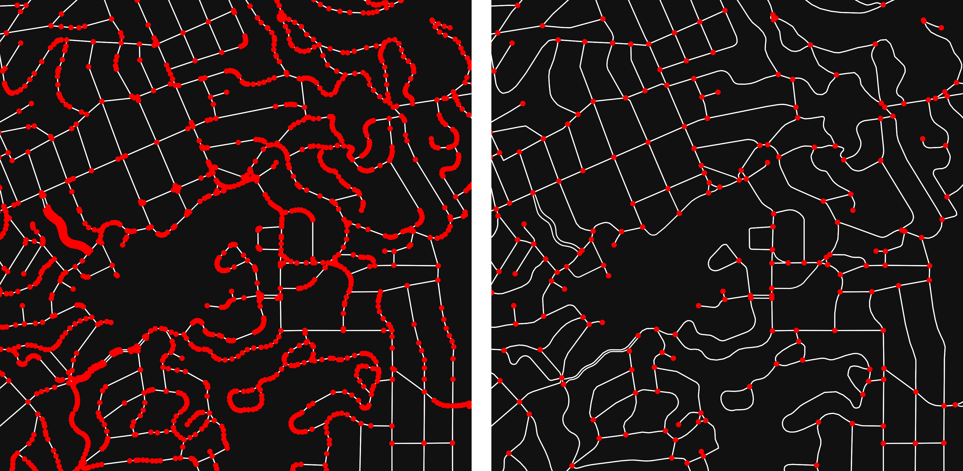
Figure 1: The graph of a town’s street network before (left) and after (right) topological simplification. Circles are nodes and lines are edges.

This yields a set of models collectively comprising over 160 million nodes and 320 million edges. For better theoretical correspondence, OSMnx next topologically simplifies the graphs to retain nodes only at true intersections and dead-ends, while retaining the true spatial geometry of each edge (i.e., street segment) between them (Boeing,, 2017). This is a crucial step before conducting analytics with OpenStreetMap network data, such as calculating intersection density or average node degree. Raw OpenStreetMap data represent nodes as geometric vertices of straight-line segments composing more complex lines. Simplification produces a model that corresponds better to graph theory and transportation geography with nodes representing intersections and dead-ends and edges representing street segments. See Figure 1. Simplification yields a final set of models collectively comprising 37 million nodes and 53 million edges.

3.3. Elevation

Next, we attach elevation above sea level to every node in every graph. These elevations come from two publicly available digital elevation models (DEMs): the Advanced Spaceborne Thermal Emission and Reflection Radiometer (ASTER) v2 and the Shuttle Radar Topography Mission (SRTM). The ASTER DEM covers the world from 83° N to 83° S at a spatial resolution of one arcsecond (roughly 30 meters at the equator). The SRTM DEM covers the world from 60° N to 56° S at a spatial resolution of three arcseconds (roughly 90 meters at the equator). The ASTER DEM is finer resolution but exhibits more noise. The SRTM DEM is coarser resolution but less noisy, and was further processed by CGIAR-CSI to fix errors and fill voids (Gorokhovich and Voustianiouk,, 2006). We additionally collect the elevation of each node using the Google Maps Elevation API, but only for validation purposes as Google provides global and high-quality but commercial and closed-source data with restrictive licensing (cf. Rusli et al.,, 2014).

On a node-by-node basis, the workflow selects either the ASTER or SRTM value to assign as the node’s elevation. It selects for each node whichever of the ASTER or SRTM elevation values has the least absolute difference from the corresponding Google value, as a validation reference point. Finally it calculates the grade (i.e., incline) of each edge then saves each urban area’s graph model to disk as a GeoPackage file, a GraphML file, and node/edge lists in comma-separated values (CSV) format.

Table 1: Fields in the indicators dataset. Those carried over from the UCD are noted as such.

Indicator Name	Type	Description
country	string	Primary country name
country_iso	string	Primary country ISO 3166-1 alpha-3 code
core_city	string	Urban area core city name
uc_id	integer	Urban area’s unique identifier in UCD
cc_avg_dir	decimal	Avg clustering coefficient (unweighted, directed)
cc_avg_undir	decimal	Avg clustering coefficient (unweighted, undirected)
cc_wt_avg_dir	decimal	Avg clustering coefficient (weighted, directed)
cc_wt_avg_undir	decimal	Avg clustering coefficient (weighted, undirected)
circuity	decimal	Ratio of street lengths to straight-line distances
elev_iqr	decimal	Interquartile range of node elevations, meters
elev_mean	decimal	Mean node elevation, meters
elev_median	decimal	Median node elevation, meters
elev_range	decimal	Range of node elevations, meters
elev_std	decimal	Standard deviation of node elevations, meters
grade_mean	decimal	Mean absolute street grade (incline)
grade_median	decimal	Median absolute street grade (incline)
intersect_count	integer	Count of physical street intersections
intersect_count_clean	integer	Count of physical street intersections (after merging nodes within 10 meters geometrically)
intersect_count_clean_topo	integer	Count of physical street intersections (after merging nodes within 10 meters topologically)
k_avg	decimal	Avg node degree (undirected)
length_mean	decimal	Mean street segment length (undirected edges), meters
length_median	decimal	Median street segment length (undirected edges), meters
length_total	decimal	Total street length (undirected edges), meters
node_count	integer	Count of nodes
orientation_entropy	decimal	Entropy of street bearings
orientation_order	decimal	Orientation order of street bearings
pagerank_max	decimal	Maximum PageRank value of any node
prop_4way	decimal	Proportion of nodes that represent 4-way street intersections
prop_3way	decimal	Proportion of nodes that represent 3-way street intersections
prop_deadend	decimal	Proportion of nodes that represent dead-ends
self_loop_proportion	decimal	Proportion of edges that are self-loops
straightness	decimal	The inverse of circuity
street_segment_count	integer	Count of street segments (undirected edges)
uc_names	string	List of city names within this urban area (UCD)
world_region	string	Major geographical region (UCD)
world_subregion	string	Minor geographical region (UCD)
resident_pop	integer	Total resident population, 2015 (UCD)
area	decimal	Area within boundary polygon, km2 (UCD)
built_up_area	decimal	Built-up surface area in 2015, km2 (UCD)

3.4. Indicator Calculation

Once the models are all assembled, we load each’s saved GraphML file with OSMnx to calculate each indicator described in Table 1. These indicators are merged with a set of essential indicators from the UCD and saved as a CSV-formatted file.

Details and descriptions are in order for the interpretability of some fields in this indicators dataset. The country field contains the name of the country in which the urban area wholly or primarily (in the case of transnational urban areas) lies, while country_iso contains its ISO 3166-1 alpha-3 code for unambiguous identification. The core_city field contains the name of the urban area’s core (typically largest) city and the uc_id field contains the unique identifier of this urban area in the UCD, allowing downstream users to join these indicators with all of those in the UCD. The uc_names field contains a list of city names within this urban area, per the UCD. The world_region and world_subregion fields contain the urban area’s major and minor geographical region, per the UCD. The resident_pop field contains the UCD’s estimated 2015 resident population in the urban area. The area and built_up_area fields contain the UCD’s boundary polygon area and built-up surface area (both in km²) respectively.

The circuity indicator is the graph’s ratio of street lengths to straight-line distances between adjacent nodes, and straightness is its inverse. The former measures how circuitous the street network is on average, whereas the latter measures how closely its streets approximate straight lines (Boeing,, 2021). The elev_mean, elev_median, elev_std, elev_iqr, and elev_range represent the calculated mean, median, standard deviation, interquartile range, and range of node elevations, in meters. These provide indicators of the topography underlying the network. The grade_mean and grade_median fields represent the calculated mean and median street grade absolute values.

The intersect_count indicator represents the number of street intersections in the urban area—that is, the number of nodes with more than two incident edges in an undirected representation of the graph. The intersect_count_clean indicator is calculated by merging intersections within 10 meter buffers of each other geometrically (i.e., 10 meter Euclidean radii) before counting them. This prevents the over-counting of complex intersections. For example, the intersection of two divided roads—each comprising two centerline one-way geometries—creates four nodes and thus would otherwise be counted as four intersections. Roundabouts similarly create multiple intersection points unless consolidated. The 10 meter parameterization has a track record in the literature (e.g. Barrington-Leigh and Millard-Ball,, 2020). The buffer could be customized for each study site to reflect local urban design standards, but for the sake of consistent interpretation across the dataset we use a universal parameterization that works relatively well across all study sites.

The intersect_count_clean_topo indicator is calculated by merging intersections within 10 meters of each other topologically along the network. This prevents topologically remote but spatially proximate nodes from being merged. For example, a street intersection may lie directly below a freeway overpass’s intersection with an on-ramp. We would not want to merge these and count them as a single intersection, even though their planar Euclidean distance is approximately zero: in reality, they are distinct junctions in the three-dimensional system of roads. Similarly, in a residential neighborhood, a bollarded street may create a dead-end immediately next to an intersection or traffic circle. We would not want to merge this dead-end with the intersection and connect their edges—they are not adjacent nodes in the graph’s topology. These examples illustrate (two-dimensional) geometric proximity, but topological remoteness. Accordingly, in some situations we may expect higher intersection counts in intersect_count_clean than intersect_count_clean_topo.

Clustering coefficients measure the extent to which a node’s neighbors form a complete graph (Jiang and Claramunt,, 2004; Opsahl and Panzarasa,, 2009). The cc_avg_dir and cc_avg_undir indicators are the urban area’s directed and undirected unweighted average clustering coefficient. The cc_wt_avg_dir and cc_wt_avg_undir indicators are its directed and undirected length-weighted average clustering coefficient. The pagerank_max indicator is the maximum PageRank value of any node in the urban area: PageRank ranks nodes’ importance based on the structure of their links (Agryzkov et al.,, 2012; Boeing, 2020a, ). The self_loop_proportion measures the urban area’s proportion of physical street segments that self-loop.

The k_avg indicator represents the average node degree of the undirected representation of the graph—that is, on average, how many physical streets (rather than directed edges) are incident to each node. The length_mean and length_median indicators are the calculated mean and median physical street segment (i.e., undirected edge) lengths in meters, representing the average and typical linear block lengths. The street_segment_count and node_count fields contain the counts of physical street segments and nodes respectively. The prop_4way, prop_3way, and prop_deadend fields contain the proportions of nodes in the graph that represent four-way intersections, three-way intersections, and culs-de-sac respectively. The orientation_entropy and orientation_order indicators represent the calculated entropy of street bearings and their linearized and normalized order, as developed in Boeing, (2019).

4. Results and Discussion

4.1. Open Data Repositories

All of the resulting street network models, indicators, and metadata have been made publicly available on the Harvard Dataverse, organized within a top-level dataverse collectively comprising approximately 80 gigabytes of data. All of these datasets are freely available for reuse: see the conclusion section for usage notes. All model files (in GeoPackage, GraphML, and node/edge list format) are compressed and zipped at the country level. The top-level dataverse contains five constituent datasets to organize the street network models, indicators, and metadata for retrieval:

• Global Urban Street Networks Indicators: contains the calculated indicators plus essential fields carried over from the UCD for use in downstream analyses. See Table 1.

• Global Urban Street Networks Metadata: contains metadata describing the indicators and the node/edge attributes in the model files.

• Global Urban Street Networks GraphML: contains all the GraphML street network model files, compressed and zipped at the country level.

• Global Urban Street Networks GeoPackages: contains all the street network model GeoPackage files, compressed and zipped at the country level.

• Global Urban Street Networks Node/Edge Lists: contains all the street network model node and edge lists in CSV file format, compressed and zipped at the country level.

4.2. Indicator Analysis

Table 2 presents the results of this workflow by aggregating and summarizing a subset of street network form indicators of particular interest to transportation researchers. It reports population-weighted mean values across all urban areas, aggregated and summarized at the level of the world subregion.

Each table column represents an indicator, some of which are transformed for presentation as follows. The Circuity Pct column subtracts 1 from the circuity indicator and expresses the result as a percent. It thus represents how much more circuitous the streets are than if they were all straight lines. The Avg Node Degree, Orientation Order, and Median Street Length columns present the k_avg, orientation_order, and length_median indicator values respectively. The Avg Grade column expresses the grade_mean indicator as a percent. The Intersect Density column divides the intersect_count_clean_topo indicator by the built_up_area indicator, and thus represents street intersections per km².

Finally, each of these indicators is aggregated at the subregion-level using the population-weighted mean. Such weighting reflects the average person’s exposure by measuring the average indicator value as experienced by the subregion’s residents within their urban areas. These population-weighted means are calculated as shown in Equation 1 where $d_{s}$ is the population-weighted mean value of indicator $d$ in subregion $s$, $n$ is the number of urban areas in subregion $s$, $i$ indexes those urban areas, $d_{i}$ is the value of indicator $d$ in urban area $i$, $p_{i}$ is the population of urban area $i$, and $p_{s}$ is the total population of subregion $s$.

$$d_{s}=\sum_{i=1}^{n}\frac{p_{i}}{p_{s}}d_{i}$$ (1)

Table 2: Aggregate analysis of urban area street network indicators worldwide: population-weighted mean values, calculated and transformed as described in the text.

World Subregion	Circuity Pct	Avg Node Degree	Orientation Order	Median Street Length	Avg Grade Pct	Intersect Density
Eastern Africa	5.28	2.80	0.12	82.87	3.19	266.88
Middle Africa	3.81	2.89	0.12	93.97	3.16	171.56
Northern Africa	3.66	2.90	0.19	49.76	2.56	284.10
Southern Africa	8.59	2.82	0.05	77.72	3.09	151.13
Western Africa	4.30	2.82	0.13	92.75	2.48	159.98
Eastern Asia	4.86	2.96	0.22	168.96	2.14	45.74
South-Central Asia	6.10	2.65	0.20	138.83	1.97	133.93
South-Eastern Asia	6.22	2.60	0.14	64.06	2.68	190.12
Western Asia	4.97	2.95	0.13	70.04	3.46	197.08
Eastern Europe	4.97	2.84	0.09	114.48	2.23	39.04
Northern Europe	6.50	2.47	0.02	65.94	2.94	97.23
Southern Europe	5.93	2.86	0.05	62.99	4.09	115.94
Western Europe	6.40	2.79	0.03	78.11	2.60	72.55
Caribbean	5.62	2.82	0.10	76.38	3.14	118.38
Central America	3.89	2.88	0.17	62.80	4.06	166.02
South America	3.68	3.03	0.15	73.22	3.85	197.76
Northern America	6.71	2.87	0.32	99.95	2.50	53.23
Australia/New Zealand	5.92	2.73	0.19	82.33	4.47	64.84
Melanesia	8.50	2.51	0.03	106.07	3.67	105.17

Southern Africa and Melanesia have the most circuitous street networks, where the weighted-average urban area has streets 8.6% and 8.5% more circuitous than straight lines. In contrast, Northern Africa and South America have the least circuitous, at 3.7% each. South America and Eastern Asia have the highest weighted-average average node degree (3.0 each), a measure of network connectedness, whereas Northern Europe and Melanesia (2.5 each) have the lowest. Orientation order, a spatial signature of coordinated central planning, is highest in Northern America (0.32) and Eastern Asia (0.22) and lowest in Northern Europe (0.02) and Melanesia (0.03).

Eastern Asia (169 meters) and South-Central Asia (139 meters) have the longest weighted-average median street segment lengths. In contrast, Northern Africa (50 meters) and Central America (63 meters) have the shortest. The weighted-average urban areas in Australia/New Zealand (4.5%) and Southern Europe (4.1%) have the highest average street grades, indicating cities built on hillier terrain, whereas Eastern (2.1%) and South-Central Asia (2.0%) have the lowest, indicating cities built on flatter land. Finally, intersection densities (topologically cleaned) are highest in Northern Africa (284/km²) and Eastern Africa (267/km²) and lowest in Eastern Europe (39/km²) and Eastern Asia (46/km²).

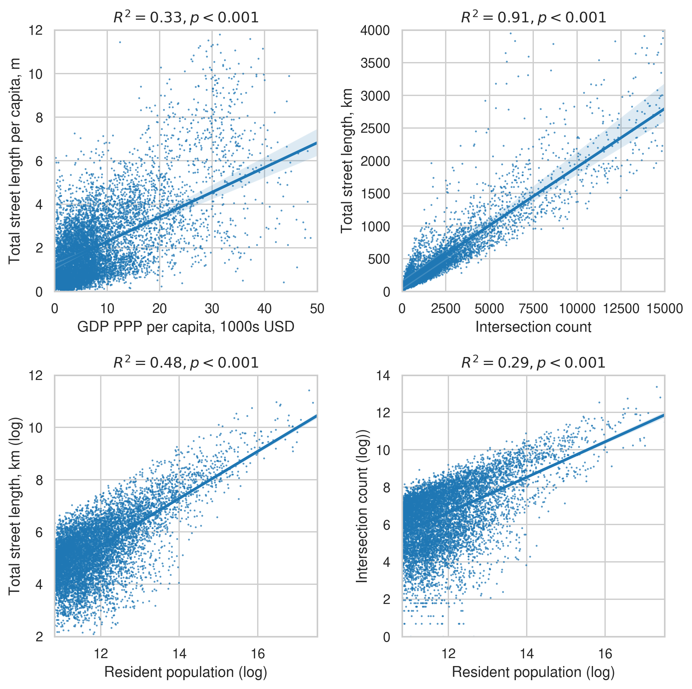
Figure 2: Scatter plots of relationships across all worldwide urban areas with bivariate regression lines and shaded 95% confidence intervals. Axes constrained to not display all outliers.

Figure 2 visualizes a set of fundamental bivariate relationships (estimated via ordinary least squares with variables transformed as needed for best linear fit) across all urban areas worldwide. Urban areas’ intersection counts (topologically cleaned) exhibit a strong linear relationship with their total street lengths (R² = 0.91, p < 0.001), as expected from theory. A 1 intersection increase in an urban area’s intersection count is associated with a 178.6 meter increase in its total street length, ±1.2 meters (margin of error at 95% confidence).

Total street length and intersection count both scale slightly sublinearly with urban area population, as seen in the log-log plots at the bottom of Figure 2. A 1% increase in urban area population is associated with a 0.90% (±0.02%) increase in total street length and a 0.95% (±0.03%) increase in intersection count, which makes theoretical sense as residents can share public infrastructure. Similar results have been found in prior studies of a single country (e.g., Bettencourt,, 2013).

Urban areas’ per capita GDP estimates (i.e., the UCD’s 2015 urban area GDP, based on purchasing power parity, in 2011 USD) exhibit a moderate linear relationship with total street length per capita. Across all urban areas, the mean per capita street length is 2.13 meters, and a $10,000 USD increase in per capita GDP is associated with a 1.13 (±0.03) meter increase in per capita street length. Per capita street length is a common indicator of a city’s “infrastructure accessibility” and this finding provides new evidence consilient with prior smaller-sample findings in the literature: cities with greater wealth and economic activity tend to have more road infrastructure (e.g., Dingil et al.,, 2018).

4.3. Validation

To be useful in urban science and practice, these models must faithfully represent the real world. Validation needs to be considered from three perspectives.

First, the source data themselves must accurately represent the real-world. In terms of study site demarcation, the UCD derives from the state-of-the-art GHSL developed in tandem by international authorities for this purpose. Numerous researchers have investigated OpenStreetMap’s urban street accuracy and completeness (Barron et al.,, 2014; Basiri et al.,, 2016; Corcoran et al.,, 2013; Girres and Touya,, 2010; Haklay,, 2010; Neis et al.,, 2011; Zielstra et al.,, 2013). These data are not perfect. Barrington-Leigh and Millard-Ball, (2017) note that OpenStreetMap was particularly incomplete in China as of 2016 due to restrictions on private surveying and publishing geospatial data. The Chinese models and indicators may in turn suffer from missing source data, and this could partly explain the low intersection density in Eastern Asia in Table 2 as China accounts for 79% of the subregion’s urban population. Nevertheless, OpenStreetMap is the current state-of-the-art for international street network analysis and represents the best available global data today.

The second validation perspective considers how well the resulting graph models represent the OpenStreetMap street network. Are the models constructed properly? Does the workflow introduce errors? The open source modeling software, OSMnx, has been downloaded and installed over 300,000 times from the Anaconda package repository, generating a large test bed of users continuously vetting its functionality. To further assess these models, this study tests the resulting repository’s data quality against the original OpenStreetMap source data as a reference dataset by adapting the methodologies of Barrington-Leigh and Millard-Ball, (2017) and Karduni et al., (2016). It randomly samples 100 US urban areas and 100 non-US urban areas then manually compares each with the OpenStreetMap source data. The results conform to expectations given the source data and OSMnx’s parameterization. Every graph model is also tested to ensure it can be loaded, analyzed, and routed, confirming that this study’s computational workflow created a functioning model as described in the methods section.

Third, the elevation data are validated by comparing the ASTER, SRTM, and Google values for each node. Across all 37 million nodes worldwide, the elevation values between these three sources exhibit high correlation (all r > 0.999, p < 0.001). Table 3 summarizes their pairwise differences. The ASTER and SRTM node elevation values differ by only 19 centimeters on average, and the median node has the same elevation value across both. The ASTER and SRTM differences with the Google validation values are greater but both the mean and median remain near or under 1 meter. The high min/max values represent noisy outliers that our node elevation selection process mitigated: across all urban areas, the median node’s selected elevation value differs from Google by only 32 centimeters. Finally, we compare our street networks’ elev_mean indicator with the UCD’s estimated average elevation for each urban area. They strongly correlate (r > 0.999, p < 0.001) and the median difference between the two is 16 centimeters. Overall, the high correlations and small pairwise differences demonstrate the tight correspondence between the different elevation values and lend confidence to using the ASTER and SRTM open data in these models.

Table 3: Summary statistics of pairwise differences in elevation (meters) from ASTER, SRTM, and Google across all nodes worldwide.

	ASTER$-$SRTM	ASTER$-$Google	SRTM$-$Google
Mean	-0.19	0.99	1.18
Std Dev	7.83	7.90	3.26
Min	-319.00	-319.01	-276.55
25%	-5.00	-3.55	-0.52
50%	0.00	1.00	0.57
75%	4.00	5.33	2.57
Max	441.00	442.34	138.83

5. Conclusion

5.1. New Models and Indicators for Street Network Science

This article presented new methods to model and analyze the street network of each urban area in the world. It used open-source tools and open data to build these models and calculate geometric and topological indicators of street network form. All of its Python source code and resulting data have been deposited in open repositories for public reuse. This represents the first such comprehensive repository of ready-to-use urban area street network models and indicators worldwide.

Analyzing these indicators reveals a snapshot of street network form around the world. We find that both total street length and intersection count scale sublinearly with urban area population. Higher per capita GDP in an urban area is associated with higher per capita total street length. We also find that elevation open data from ASTER and SRTM compare well to Google’s closed source, commercial data. All three sources’ elevation values correlate strongly. The median pairwise difference between the nodes’ elevation values and the Google validation values is only 32 centimeters, and the median pairwise difference between the urban areas’ mean street network elevations and the UCD mean elevations is only 16 centimeters.

The open data repositories generated by this study fill two needs in the research community. First, the network models allow researchers to quickly engage in graph-theoretic street network analyses worldwide without first spending weeks writing their own ad hoc code for data collection and modeling. Second, the indicators data provide the first comprehensive worldwide set of geometric and topological street network form indicators at the urban area scale. Together, these results help democratize street network science, opening up quantitative analyses to urban planners and policymakers with less-technical backgrounds who otherwise may struggle to develop a complete computational analytics workflow themselves.

While OpenStreetMap itself provides incredibly valuable raw data, this project transforms these data into ready-to-use models and indicators through substantial processing. For example, these topologically simplified graphs provide models that correspond much better to graph theory and transportation geography than raw OpenStreetMap data do, and they are much faster to run graph algorithms on because most such algorithms scale with node count. They also include elevation and grade data, which are very sparse on OpenStreetMap and are too often ignored in street network analytics. Researchers and practitioners can use these models to simulate trips, assess network vulnerability to flooding and sea level rise, or measure accessibility to points of interest.

The indicators data offer a useful basket of variables for cross-sectional, worldwide studies of street network form, and the topologically-consolidated intersection counts and densities contribute a more theoretically-sound measure than traditional node counts or purely geometric consolidation can. Researchers and practitioners can use these indicators to estimate relationships between street network characteristics and transport-sector greenhouse gas emissions around the world, compare per capita road infrastructure provision across urban areas, or scorecard different cities’ street network compactness and connectivity for sustainability initiatives.

5.2. How to Use These Models and Indicators

Finally, this article concludes with a few notes on reuse. The indicators data can be loaded with any data analysis tool. The street network models can be loaded with most GIS and network analysis tools, including OSMnx.

Each graph model file is named as city_name-uc_id.extension, where uc_id is the urban area’s unique identifier in the UCD. The uc_id field thus links each graph model file to its urban area in the UCD as well as to its row in the indicators dataset. For example, within the china-CHN.zip file from the Global Urban Street Networks GraphML repository are all of China’s urban areas’ GraphML files, including beijing-10687.graphml. This GraphML file contains the street network model of Beijing and its uc_id is 10687. As such, 10687 is Beijing’s unique identifier in the indicators dataset and in the UCD.

All of the code used for modeling and analysis in this study is open source and available on GitHub for public inspection, adaptation, and reuse. Comprehensive documentation of OSMnx and its modules and functions used in this study is available online and OSMnx usage examples, tutorials, and demonstrations are available on GitHub for users interested in working with this toolkit.

References

- Agryzkov et al., (2012) Agryzkov, T., Oliver, J. L., Tortosa, L., and Vicent, J. F. (2012). An algorithm for ranking the nodes of an urban network based on the concept of PageRank vector. Applied Mathematics and Computation, 219(4):2186–2193.
- Barrington-Leigh and Millard-Ball, (2017) Barrington-Leigh, C. and Millard-Ball, A. (2017). The world’s user-generated road map is more than 80% complete. PLOS ONE, 12(8):e0180698.
- Barrington-Leigh and Millard-Ball, (2019) Barrington-Leigh, C. and Millard-Ball, A. (2019). A global assessment of street-network sprawl. PLOS ONE, 14(11):e0223078.
- Barrington-Leigh and Millard-Ball, (2020) Barrington-Leigh, C. and Millard-Ball, A. (2020). Global trends toward urban street-network sprawl. Proceedings of the National Academy of Sciences, 117(4):1941–1950.
- Barron et al., (2014) Barron, C., Neis, P., and Zipf, A. (2014). A Comprehensive Framework for Intrinsic OpenStreetMap Quality Analysis. Transactions in GIS, 18(6):877–895.
- Barthelemy, (2011) Barthelemy, M. (2011). Spatial Networks. Physics Reports, 499(1-3):1–101.
- Basiri et al., (2016) Basiri, A., Jackson, M., Amirian, P., Pourabdollah, A., Sester, M., Winstanley, A., Moore, T., and Zhang, L. (2016). Quality assessment of OpenStreetMap data using trajectory mining. Geospatial Information Science, 19(1):56–68.
- Batty, (2005) Batty, M. (2005). Network geography: Relations, interactions, scaling and spatial processes in GIS. In Unwin, D. J. and Fisher, P., editors, Re-Presenting GIS, pages 149–170. John Wiley & Sons, Chichester, England.
- Bettencourt, (2013) Bettencourt, L. (2013). The Origins of Scaling in Cities. Science, 340(6139):1438–1441.
- Boeing, (2017) Boeing, G. (2017). OSMnx: New Methods for Acquiring, Constructing, Analyzing, and Visualizing Complex Street Networks. Computers, Environment and Urban Systems, 65:126–139.
- Boeing, (2019) Boeing, G. (2019). Urban Spatial Order: Street Network Orientation, Configuration, and Entropy. Applied Network Science, 4(1):67.
- (12) Boeing, G. (2020a). A Multi-Scale Analysis of 27,000 Urban Street Networks: Every US City, Town, Urbanized Area, and Zillow Neighborhood. Environment and Planning B: Urban Analytics and City Science, 47(4):590–608.
- (13) Boeing, G. (2020b). The Right Tools for the Job: The Case for Spatial Science Tool-Building. Transactions in GIS, 24(5):1299–1314.
- Boeing, (2021) Boeing, G. (2021). Off the Grid…and Back Again?: The Recent Evolution of American Street Network Planning and Design. Journal of the American Planning Association, 87(1):123–137.
- Brandes and Erlebach, (2005) Brandes, U. and Erlebach, T., editors (2005). Network analysis: methodological foundations. Number 3418 in Lecture Notes in Computer Science. Springer, Berlin, Germany.
- Cardillo et al., (2006) Cardillo, A., Scellato, S., Latora, V., and Porta, S. (2006). Structural properties of planar graphs of urban street patterns. Physical Review E, 73(6).
- Corcoran et al., (2013) Corcoran, P., Mooney, P., and Bertolotto, M. (2013). Analysing the growth of OpenStreetMap networks. Spatial Statistics, 3:21–32.
- da Cruz et al., (2020) da Cruz, N. F., Oh, D. Y., and Choumar, N. B. (2020). The metropolitan scale. Cities, 100:102644.
- Dingil et al., (2018) Dingil, A. E., Schweizer, J., Rupi, F., and Stasiskiene, Z. (2018). Transport indicator analysis and comparison of 151 urban areas, based on open source data. European Transport Research Review, 10(2):58.
- Florczyk et al., (2019) Florczyk, A., Melchiorri, M., Corbane, C., Schiavina, M., Maffenini, M., Pesaresi, M., Politis, P., Sabo, S., Freire, S., Ehrlich, D., Kemper, T., Tommasi, P., Airaghi, D., and Zanchetta, L. (2019). Description of the GHS Urban Centre Database 2015, Public Release 2019, Version 1.0. Publications Office of the European Union, Luxembourg. doi:10.2760/037310.
- Gastner and Newman, (2006) Gastner, M. T. and Newman, M. E. J. (2006). The spatial structure of networks. The European Physical Journal B: Condensed Matter and Complex Systems, 49(2):247–252.
- Girres and Touya, (2010) Girres, J.-F. and Touya, G. (2010). Quality Assessment of the French OpenStreetMap Dataset. Transactions in GIS, 14(4):435–459.
- Gorokhovich and Voustianiouk, (2006) Gorokhovich, Y. and Voustianiouk, A. (2006). Accuracy assessment of the processed SRTM-based elevation data by CGIAR using field data from USA and Thailand and its relation to the terrain characteristics. Remote Sensing of Environment, 104(4):409–415.
- Graham et al., (2015) Graham, M., De Sabbata, S., and Zook, M. A. (2015). Towards a study of information geographies: (im)mutable augmentations and a mapping of the geographies of information: Towards a study of information geographies. Geo: Geography and Environment, 2(1):88–105.
- Haklay, (2010) Haklay, M. (2010). How Good is Volunteered Geographical Information? A Comparative Study of OpenStreetMap and Ordnance Survey Datasets. Environment and Planning B: Planning and Design, 37(4):682–703.
- Hopcroft and Tarjan, (1974) Hopcroft, J. and Tarjan, R. (1974). Efficient Planarity Testing. Journal of the ACM, 21(4):549–568.
- Jiang and Claramunt, (2004) Jiang, B. and Claramunt, C. (2004). Topological Analysis of Urban Street Networks. Environment and Planning B: Planning and Design, 31(1):151–162.
- Jokar Arsanjani et al., (2015) Jokar Arsanjani, J., Zipf, A., Mooney, P., and Helbich, M., editors (2015). OpenStreetMap in GIScience. Springer International, Cham, Switzerland.
- Karduni et al., (2016) Karduni, A., Kermanshah, A., and Derrible, S. (2016). A protocol to convert spatial polyline data to network formats and applications to world urban road networks. Scientific Data, 3:160046.
- Lemoine-Rodríguez et al., (2020) Lemoine-Rodríguez, R., Inostroza, L., and Zepp, H. (2020). The global homogenization of urban form: An assessment of 194 cities across time. Landscape and Urban Planning, 204:103949.
- Maier, (2014) Maier, G. (2014). OpenStreetMap, the Wikipedia Map. Region, 1(1):R3–R10.
- Marshall et al., (2018) Marshall, S., Gil, J., Kropf, K., Tomko, M., and Figueiredo, L. (2018). Street Network Studies: from Networks to Models and their Representations. Networks and Spatial Economics, 18:735–749.
- Masucci et al., (2009) Masucci, A. P., Smith, D., Crooks, A., and Batty, M. (2009). Random planar graphs and the London street network. The European Physical Journal B: Condensed Matter and Complex Systems, 71(2):259–271.
- Neis et al., (2011) Neis, P., Zielstra, D., and Zipf, A. (2011). The Street Network Evolution of Crowdsourced Maps: OpenStreetMap in Germany 2007–2011. Future Internet, 4(1):1–21.
- Newman, (2003) Newman, M. E. J. (2003). The Structure and Function of Complex Networks. SIAM Review, 45(2):167–256.
- Newman, (2010) Newman, M. E. J. (2010). Networks: An Introduction. Oxford University Press, Oxford, England.
- Opsahl and Panzarasa, (2009) Opsahl, T. and Panzarasa, P. (2009). Clustering in weighted networks. Social Networks, 31(2):155–163.
- O’Sullivan, (2014) O’Sullivan, D. (2014). Spatial Network Analysis. In Fischer, M. M. and Nijkamp, P., editors, Handbook of Regional Science, pages 1253–1273. Springer-Verlag, Berlin, Germany.
- (39) Porta, S., Crucitti, P., and Latora, V. (2006a). The Network Analysis of Urban Streets: A Dual Approach. Physica A: Statistical Mechanics and its Applications, 369(2):853–866.
- (40) Porta, S., Crucitti, P., and Latora, V. (2006b). The network analysis of urban streets: a primal approach. Environment and Planning B: Planning and Design, 33(5):705–725.
- Ratti, (2004) Ratti, C. (2004). Space syntax: some inconsistencies. Environment and Planning B: Planning and Design, 31(4):487–499.
- Rusli et al., (2014) Rusli, N., Majid, M. R., and Din, A. H. M. (2014). Google Earth’s derived digital elevation model: A comparative assessment with Aster and SRTM data. IOP Conference Series: Earth and Environmental Science, 18:012065.
- Schmidt and Klettner, (2013) Schmidt, M. and Klettner, S. (2013). Gender and Experience-Related Motivators for Contributing to OpenStreetMap. In AGILE 2013, Leuven, Belgium. AGILE.
- Sehra et al., (2020) Sehra, S. S., Singh, J., Rai, H. S., and Anand, S. S. (2020). Extending Processing Toolbox for Assessing the Logical Consistency of OpenStreetMap Data. Transactions in GIS, 24(1):44–71.
- Székely, (2004) Székely, L. A. (2004). A successful concept for measuring non-planarity of graphs: the crossing number. Discrete Mathematics, 276(1-3):331–352.
- Trudeau, (1994) Trudeau, R. J. (1994). Introduction to Graph Theory. Dover Publications, New York, NY, 2nd edition.
- Vespignani, (2018) Vespignani, A. (2018). Twenty years of network science. Nature, 558:528–529.
- Viana et al., (2013) Viana, M. P., Strano, E., Bordin, P., and Barthelemy, M. (2013). The simplicity of planar networks. Scientific Reports, 3(3495):1–6.
- Zielstra et al., (2013) Zielstra, D., Hochmair, H. H., and Neis, P. (2013). Assessing the Effect of Data Imports on the Completeness of OpenStreetMap – A United States Case Study. Transactions in GIS, 17(3):315–334.