Inexact restoration for derivative-free expensive function minimization and applications

Abstract

The Inexact Restoration approach has proved to be an adequate tool for handling the problem of minimizing an expensive function within an arbitrary feasible set by using different degrees of precision. This framework allows one to obtain suitable convergence and complexity results for an approach that rationally combines low- and high-precision evaluations. In this paper we consider the case where the domain of the optimization problem is an abstract metric space. Assumptions about differentiability or even continuity will not be used in the general algorithm based on Inexact Restoration. Although optimization phases that rely on smoothness cannot be used in this case, basic convergence and complexity results are recovered. A new derivative-free optimization phase is defined and the subproblems that arise at this phase are solved using a regularization approach that takes advantage of different notions of stationarity. The new methodology is applied to the problem of reproducing a controlled experiment that mimics the failure of a dam.

Key words: Nonlinear programming, Inexact Restoration, derivative-free, inexact evaluation of expensive function, algorithms.

2010 Mathematics Subject Classification: 65K05, 65K10, 90C30, 90C56, 65Y20, 90C90.

1 Introduction

For many reasons scientists and engineers may need to optimize problems in which the objective function is very expensive to evaluate. In these cases, partial, and obviously inexact, evaluations are useful. The idea is to decrease as much as possible functional values using partial evaluations in such a way that, when we have no choice except to evaluate the function with maximal accuracy, we are already close enough to a solution of the problem. Rational decisions about when to increase accuracy (and evaluation cost) or even when to try more inexact evaluations are hard to make. Roughly speaking, we need a compromise between accuracy of evaluation and functional decrease that is difficult to achieve on a mere heuristic basis.

Most papers on minimization methods with inexact evaluations aim to report the behavior of modifications of standard algorithms in the presence of errors in the computation of the objective function, its derivatives, or the constraints [5, 6, 41, 34, 22, 35, 33]. In general, it is assumed that the objective function and, perhaps its derivatives, can be computed with a given error bound each time the functional value is required at an arbitrary point. In [5], the underlying “exact” algorithm is based on adaptive regularization. Trust-region algorithms inspired in [24, §10.6] are addressed in [35]. High-order complexity of stochastic regularization is considered in [6]. The case of PDE-constrained optimization is studied in [41]. Nonsmoothness is addressed in [34]. Convex quadratic problems using Krylov methods are studied in [33]. Many of these works seem to be influenced by an early paper by Carter [22].

In recent papers [9, 10, 42], a methodology based on the analogy of the Inexact Restoration idea for continuous constrained optimization and the process of increasing accuracy of function evaluations was developed. In this approach, it is not assumed that one is able to compute a functional value (let alone derivatives) within a given required error bound. Instead, it is assumed that accuracy is represented by an abstract function $h(y)$ such that $h(y)=0$ means maximal accuracy and $y$ is a case-dependent procedure. For instance, $y\in Y$ may represent an algorithm with which one can compute the approximate objective function and $h(y)\geq 0$ is an accuracy-related function. The connection between the value of $h(y)$ and a possible error bound is not assumed to be known. For example, $y$ may represent the maximal number of iterations that are allowed for a numerical algorithm that computes the objective function before obtaining convergence when we know that convergence eventually occurs but an error estimation is not available. Several additional examples may be found in [10].

Inexact Restoration methods for smooth constrained optimization were introduced in [45]. Each iteration of an Inexact Restoration method proceeds in two stages. In the Restoration Phase, infeasibility is reduced; and, in the Optimization Phase, the reduction of the objective function or its Lagrangian is addressed with a possible loss of feasibility. Convergence with sharp Lagrangians as merit functions was proved in [44]. Applications to bilevel programming were given in [46, 1]. In [20], an application to multiobjective optimization was described. The first line-search implementation was introduced in [28]. Nonsmooth versions of the main algorithms were defined in [2, 25, 27]. The employment of filters associated with Inexact Restoration was exploited in [36, 25]. Applications to control problems were given in [38, 12, 37, 3]. In [26], Inexact Restoration was used to obtain global convergence of a sequential programming method. Large-scale applications were discussed in [32]. In [31], Inexact Restoration was used for electronic structure calculations; and problems with a similar mathematical structure were addressed in [30]. The reliability of Inexact Restoration for arbitrary nonlinear optimization problems was assessed in [8]. In [21], the worst-case evaluation complexity of Inexact Restoration was analyzed. An application to finite-sum minimization was described in [7]. Continuous and discrete variables were considered in [11]. Non-monotone alternatives were defined in [29]. An application to the demand adjustment problem was given in [49]. Local convergence results were proved in [12].

In [10], an algorithm of Inexact Restoration type applied to minimization with inexact evaluations that exhibits convergence and complexity results, was developed. However, the algorithm proposed in [10], as well as the algorithms previously introduced in [9, 42], employs derivatives of the objective function, a feature that may be inadequate in many cases in which one does not have differentiability at all. This state of facts motivates the present work. Here, the algorithms of [9, 10, 42] are adapted to the case in which derivatives are not available and the main theoretical results are proved. In addition, the domain of the optimization problem is considered to be a metric space, unlike an Euclidean space as considered in [9, 10, 42]. The reason why we are proposing the generalization to metric spaces is simple: Many real optimization problems take place in domains that are not Euclidean spaces and, many times, in domains that are not even vector spaces. Naturally, there is a price we pay for this generalization because there are no known optimality conditions that can be invoked to define possible approximate solutions to the problems. In the current state of development of methods for optimization in metric spaces, it is natural that the optimality conditions that we can define are inspired by what happens in Euclidean spaces. In that sense, we emphasize a poorly known or poorly exploited property: In the Euclidean case, a point being a local minimizer does not imply that that point is also a local minimizer of a high-order approximation of the objective function. (For example, $(0,0)$ is a minimizer of $x_{2}^{2}-x_{1}^{3}x_{2}+x_{1}^{6}$ but is not a local minimizer of its Taylor approximation $x_{2}^{2}-x_{1}^{3}x_{2}$.) That implication is only valid when the dimension of the space is 1 or when the approximation is of order 2. If we deal with higher order approximations, the fact that a point is a local minimizer only implies that it is also a local minimizer of a suitably regularized Taylor approximation. That is the reason why, in the case of metric spaces, we cannot establish stronger necessary conditions than those mentioned in the present article. With these limitations, we elaborate the possible theory that frames affordable and reasonably efficient techniques. Moreover, in the present work, we focus on a practical problem related with the prediction and mitigation of the consequences of dam breaking disasters.

The rest of this paper is organized as follows. The main contributions of the paper are surveyed in Section 2. The basic Inexact Restoration algorithm for problems with inexact evaluation without error bounds is introduced in Section 3. This algorithm is the one described in [10] with the difference that the domain $\Omega$ is an arbitrary metric space here, instead of a subset of $\mathbb{R}^{n}$. This extension may be useful for cases in which we have discrete or qualitative variables or when the original problem is formulated on a functional space. The proofs of the complexity and convergence results for this algorithm are similar to the ones reported in [10]. Since the employment of derivatives is essential for the definition of the Optimization Phase in [10], in the present contribution we need a different approach for that purpose. This is the subject of Section 4. The Optimization Phase requires sufficient descent of an iteration-dependent inexactly evaluated function. Sufficient descent of this function is equivalent to simple descent of an associated forcing function, therefore the required sufficient descent may be obtained by applying an arbitrary number of iterations of an ad hoc monotone minimization algorithm to an associated forcing function. This monotone algorithm, that depends on characteristics of the function being minimized, is called MOA (Monotone Optimization Algorithm) in the rest of the paper. In this phase, we may take advantage of the theoretically justified possibility of relaxing precision. In Section 5, we concentrate at the definition of a strategy for MOA. Our choice is to solve the problem addressed by MOA by means of suitable surrogate models associated with iterated adaptive regularization. Theoretical results of the previous sections are summarized in Section 6. In Section 7, we describe an implementation that is adequate for the practical problem that we have in mind. The idea is to simulate a small-scale controlled physical experiment that mimics the failure of a dam, described in [23]. We rely on an MPM-like (Moving Particles Method) approach in which the dynamic of the particles is governed by the behavior of the Spectral Projected Gradient (SPG) method applied to the minimization of a semi-physical energy. Our optimization problem consists of finding the parameters of the energy function by means of which the trajectory of the SPG method best reproduces physical experiments reported in [23]. In Section 8, we state conclusions and lines for future research.

Notation. $\mathbb{N}_{+}$ denotes the non-negative integer numbers; while $\mathbb{R}_{+}$ denotes the non-negative real numbers. The symbol $\|\cdot\|$ denotes the Euclidean norm of vector and matrices.

2 Main problem and contributions

Consider the problem

$$\mbox{Minimize (with respect to $x$) }f(x,y)\mbox{ subject to }h(y)=0\mbox{ and }x\in\Omega,$$ (1)

where $\Omega$ is an arbitrary metric space, $Y$ is an abstract set, $h:Y\to\mathbb{R}_{+}$, and $f:\Omega\times Y\to\mathbb{R}$. For further reference, $d(x,z)$ denotes the distance between $x$ and $z$ in $\Omega$. $Y$ is sometimes interpreted as a set of indices according to which the objective function is computed with different levels of accuracy. The nature of these indices varies with the problem and, for this reason, $Y$ is presented as an arbitrary set. The function $h(y)$ is assumed to be related with the accuracy in the evaluation of $f$ associated with the index $y\in Y$. The smaller the value of $h(y)$, the higher the accuracy; while maximal accuracy corresponds to $h(y)=0$. In principle, problem (1) consists of minimizing the objective function with maximal accuracy.

In this article, the domain $\Omega$ of the optimization problem (1) is a metric space, opposed to our previous paper [10], where it was the Euclidean space or a subset of it. We have in mind, therefore, spaces formed by functions in which it is possible to define a metric, and optimization problems defined on discrete sets. Because of this level of generality, the objective function $f$ can rarely be computed exactly, so inaccurate evaluations are unavoidable. However, there are many ways to deal with inaccuracy of functional evaluations. In this article each instance of inaccurate evaluation is identified by an element $y$ of an abstract set $Y$. For example, if the evaluation of the function comes from an iterative process, each $y$ can be identified with the maximum number of iterations allowed. If the evaluation depends on a discretization grid, $Y$ is the set of all possible grids. To each $y$, a “score” $h(y)$ is attributed such that $h(y)=0$ corresponds to the exact evaluation of the objective function while $h(y)>0$ corresponds to different degrees of inaccuracy; and the smaller the value of $h(y)$, the higher the evaluation accuracy. Therefore, problem (1) consists in minimizing $f(x,y)$ with respect to $x\in\Omega$, restricted to $h(y)=0$.

The evaluation of $f(x,y)$ when $h(y)=0$ is very often impossible or extremely expensive, therefore, we must rely on evaluations of $f(x,y)$ with $h(y)$ small. However, the cost of evaluating $f(x,y)$ generally increases as $h(y)$ decreases. Therefore, the strategy for solving problem (1) relies on solving problems of the form “Minimize $f(x,y_{k})$” with $h(y_{k})\to 0$. A rational way of doing this has been defined in [10] for the case in which the domain is Euclidean and is extended here to the general case.

Clearly, with this level of generality differentiability arguments are out of question and we need “derivative-free” procedures for the (approximate) minimization of $f(x,y_{k})$. For this purpose we consider that the objective function may be approximated, at each iteration, by a suitable model and that approximate minimization of such model is affordable. The precise determination of the model is, of course, problem-dependent. Under suitable assumptions, we prove that, in finite time, it is possible to obtain good approximations to a solution of problem (1). Finally, we present a practical application that concerns fitting models of dam breaking.

3 Main algorithm

In this section, the problem, the algorithm, and the convergence results introduced in [10] are revisited. Of note is that in the present contribution the domain of the problem is a general metric space instead of a subset of $\mathbb{R}^{n}$. The proofs of the theorems presented in this section are analogous to the ones given in [10], with the occurrences of $\|x-z\|$ replaced by the distance $d(x,z)$ between $x$ and $z$.

Let us define a merit function $\Phi:\Omega\times Y\times(0,1)\to\mathbb{R}$ by

$$\Phi(x,y,\theta)=\theta f(x,y)+(1-\theta)h(y).$$

The merit function $\Phi$ combines objective function evaluation and accuracy level. Here, $f(x,y)$ is the value of the objective function for a feasible $x$ when the accuracy level is determined by $y\in Y$. Therefore, $\Phi(x,y,\theta)$ represents a compromise between optimality and accuracy. The penalty parameter $\theta$ is updated at each iteration of the main algorithm. The main algorithm, with an Optimization Phase different from the one of the algorithm introduced in [10], follows.

Algorithm 3.1. Let $x_{0}\in\Omega$, $y_{0}\in Y$, $\theta_{0}\in(0,1)$, $\nu>0$, $r\in(0,1)$, $\alpha>0$, and $\beta>0$ be given. Set $k\leftarrow 0$.

Step 1.

Restoration phase

Define $y^{\mathrm{re}}_{k}\in Y$ in such a way that

$$h(y^{\mathrm{re}}_{k})\leq rh(y_{k})$$ (2)

and

$$f(x_{k},y^{\mathrm{re}}_{k})\leq f(x_{k},y_{k})+\beta h(y_{k}).$$ (3)

Step 2.

Updating the penalty parameter

If

$$\Phi(x_{k},y^{\mathrm{re}}_{k},\theta_{k})\leq\Phi(x_{k},y_{k},\theta_{k})+\frac{1-r}{2}\left(h(y^{\mathrm{re}}_{k})-h(y_{k})\right),$$ (4)

set $\theta_{k+1}=\theta_{k}$. Otherwise, set

$$\theta_{k+1}=\frac{(1+r)\left(h(y_{k})-h(y^{\mathrm{re}}_{k})\right)}{2\left(f(x_{k},y^{\mathrm{re}}_{k})-f(x_{k},y_{k})+h(y_{k})-h(y^{\mathrm{re}}_{k})\right)}.$$ (5)

Step 3.

Optimization phase

Compute $y_{k+1}\in Y$ and $x_{k+1}\in\Omega$, such that

$$f(x_{k+1},y_{k+1})\leq f(x_{k},y^{\mathrm{re}}_{k})-\alpha d(x_{k},x_{k+1})^{\nu}$$ (6)

and

$$\Phi(x_{k+1},y_{k+1},\theta_{k+1})\leq\Phi(x_{k},y_{k},\theta_{k+1})+\frac{1-r}{2}\left(h(y^{\mathrm{re}}_{k})-h(y_{k})\right).$$ (7)

Update $k\leftarrow k+1$, and go to Step 1.

Given an iterate $(x_{k},y_{k})$, at Step 1 we compute the function with an accuracy determined by $y^{\mathrm{re}}_{k}\in Y$, which is better than the accuracy given by $y_{k}$. At Step 2 we update the penalty parameter with the aim of decreasing the merit function at the restored pair $(x_{k},y^{\mathrm{re}}_{k})$ with respect to the merit function computed at $(x_{k},y_{k})$. This is typical in Inexact Restoration methods for constrained optimization. Note that, using (2), (3), the negation of (4), and the fact that $\theta_{k}>0$, it is easy to show that both the numerator and the denominator of (5) are positive and that $\theta_{k+1}\in(0,\theta_{k}]$. At Step 3 (optimization phase), we compute the new iterate, at which the objective function value should decrease with respect to the restored pair in the sense of (6) and the merit function should be improved with respect to $(x_{k},y_{k})$ in the sense of (7).

The theoretical results below describe the properties of Algorithm 3.1 and the generated sequence of iterates. These results state the algorithm is well-defined and that any desired accuracy level, for the evaluation of the objective function, can be reached in a finite number of iterations. (In fact, a complexity result is presented and an upper bound on the number of iterations is given.) A first step towards an optimality result, including complexity bounds, is also given. The optimality results will be completed in the remaining of the work with the definition of a particular strategy for computing $x_{k+1}$ and $y_{k+1}$ at Step 3 and the analysis of its convergence properties.

In Assumption 3.1 we state that defining $y^{\mathrm{re}}_{k}$ satisfying (2) and (3) at Step 1 of Algorithm 3.1 is always possible. Notice that assuming we can define $y^{\mathrm{re}}_{k}$ satisfying (2) is a simple assumption, since it corresponds to assuming that we have the capability of increasing the accuracy for the evaluation of the objective function. On the other hand, the capability of making the defined $y^{\mathrm{re}}_{k}$ to satisfy (3) is problem-dependent; and plausible choices are given in [10]. In Assumption 3.2, basic assumptions on functions $h$ and $f$ are stated.

Assumption 3.1

At Step 1 of Algorithm 3.1, for all $k\in\mathbb{N}_{+}$ it is possible to compute, in finite time, $y^{\mathrm{re}}_{k}$ satisfying (2) and (3).

Lemma 3.1

Suppose that Assumption 3.1 holds. Then, Algorithm 3.1 is well defined.

Proof: Replace, in Lemma 2.3 of [10], the occurrences of $\|x-z\|$ with $d(x,z)$. $\Box$

Assumption 3.2

There exist $h_{\max}>0$ and $f_{\min}\in\mathbb{R}$ such that, for all $y\in Y$ and $x\in\Omega$ we have that $h(y)\leq h_{\max}$ and $f(x,y)\geq f_{\min}$.

Theorem 3.1

Suppose that Assumptions 3.1 and 3.2 hold. Given $\varepsilon_{\mathrm{feas}}>0$, the number of indices $k$ such that $h(y_{k})>\varepsilon_{\mathrm{feas}}$ is bounded above by

$$\frac{c_{\mathrm{feas}}}{\varepsilon_{\mathrm{feas}}},$$ (8)

where $c_{\mathrm{feas}}$ only depends on $x_{0}$, $y_{0}$, $r$, $\theta_{0}$, $\beta$, $h_{\max}$, and $f_{\min}$.

Proof: This proof follows as the one of Corollary 2.2 of [10] with the replacements stated in the proof of Lemma 3.1. $\Box$

Theorem 3.2

Suppose that Assumptions 3.1 and 3.2 hold. Then, the series $\sum_{k=0}^{\infty}d(x_{k},x_{k+1})^{\nu}$ is convergent. Moreover, given $\varepsilon_{\mathrm{dist}}>0$, the number of iterates $k$ at which $d(x_{k},x_{k+1})>\varepsilon_{\mathrm{dist}}$ is not bigger than

$$\frac{c_{\mathrm{dist}}}{\varepsilon_{\mathrm{dist}}^{\nu}},$$ (9)

where $c_{\mathrm{dist}}$ only depends on $\alpha$, $x_{0}$, $y_{0}$, $r$, $\theta_{0}$, $\beta$, $h_{\max}$, and $f_{\min}$.

Proof: See Theorem 2.2 and Corollary 2.3 of [10] and perform the substitutions of the norm of differences with appropriate distances. $\Box$

Theorem 3.3

Suppose that Assumptions 3.1 and 3.2 hold. Then,

$$\lim_{k\to\infty}h(y_{k})=0.$$ (10)

Moreover, if $\Omega$ is complete and $\nu\leq 1$, the sequence $\{x_{k}\}$ is convergent.

Proof: The property (10) follows from Theorem 3.1. By the convergence of the series $\sum_{k=0}^{\infty}d(x_{k},x_{k+1})^{\nu}$ with $\nu\leq 1$ we have that $\{x_{k}\}$ is a Cauchy sequence. Since $\Omega$ is complete it turns out that $\{x_{k}\}$ is convergent. $\Box$

The convergence of the sequence $\{x_{k}\}$ when $\nu\leq 1$ had not been considered in [10]. In general, in nonconvex optimization, it is proved that every convergent subsequence of the sequence generated by an algorithm has optimality properties but convergence of the whole sequence is rarely obtained. The validity of the theorem does not necessarily lead us to use $\nu\leq 1$ in numerical computations, since, on the one hand, the convergence to zero of the distance between consecutive iterates is, in general, a good indication of optimality and, on the other hand, values of $\nu$ greater than 1 do not prevent the total sequence from being convergent.

4 A general framework for the Optimization Phase

In this section, we consider the implementation of Step 3 of Algorithm 3.1. Obviously, if, for any given precision parameter $y_{k+1}$, we apply any monotone optimization algorithm (MOA) to the minimization of $f(x,y_{k+1})+\alpha d(x_{k},x)^{\nu}$ subject to $x\in\Omega$, starting with $x_{k}$ as initial approximation, we find $x\in\Omega$ such that

$$f(x,y_{k+1})\leq f(x_{k},y_{k+1})-\alpha d(x_{k},x)^{\nu}.$$

This follows from the fact that even $x=x_{k}$ satisfies such inequality. However this is not a guarantee for the fulfillment of

$$f(x,y_{k+1})\leq f(x_{k},y^{\mathrm{re}}_{k})-\alpha d(x_{k},x)^{\nu}.$$ (11)

and

$$\Phi(x,y_{k+1},\theta_{k+1})\leq\Phi(x_{k},y_{k},\theta_{k+1})+\frac{1-r}{2}\left(h(y^{\mathrm{re}}_{k})-h(y_{k})\right),$$ (12)

as required at Step 3 of Algorithm 3.1. Therefore, before accepting the “solution” obtained by MOA as new iterate $x_{k+1}$, we must test whether (11) and (12) hold. If (11) and (12) hold, then we accept $x_{k+1}=x$. Otherwise, if after a finite number of trials with arbitrary $y_{k+1}$ we fail to find $x$ satisfying (11) and (12), we discard the MOA solution $x$ and apply MOA to the minimization of $f(x,y^{\mathrm{re}}_{k})+\alpha d(x_{k},x)^{\nu}$. This time, the “solution” obtained by MOA necessarily yields the fulfillment of (11) and (12) and we may accept $y_{k+1}=y^{\mathrm{re}}_{k}$ and $x_{k+1}=x$. Two natural questions arise:

1. Why not using directly $y_{k+1}=y^{\mathrm{re}}_{k}$, instead of trying first one or more different precision parameters $y_{k+1}$?

2. Which stopping criterion should we use for MOA?

The answer to the first question is the following: We normally want to choose $y_{k+1}\neq y^{\mathrm{re}}_{k}$ in such a way that $h(y_{k+1})>h(y^{\mathrm{re}}_{k})$ because $h(y^{\prime})>h(y)$ generally implies that the cost of evaluating the objective function with precision given by $y^{\prime}$ is smaller than the cost of evaluating the objective function with precision defined by $y$. In other words, we want to obtain the maximum possible progress without unnecessary evaluation effort. The answer to the second question is problem-dependent. Roughly speaking, we assume that MOA is equipped with a stopping criterion related to optimality. Recall that we are dealing with metric spaces in which nothing similar to KKT conditions exists. The idea of using an auxiliary algorithm for the fulfillment of descent conditions in the Optimization Phase of Inexact Restoration comes from [18], where Generating Set Search algorithms [40, 39] were employed as subalgorithms for an Inexact Restoration method for derivative-free optimization with smooth constraints.

Summing up, the strategy to compute $y_{k+1}\in Y$ and $x_{k+1}\in\Omega$ at Step 3 of Algorithm 3.1 is described by Algorithm 4.1 below.

Algorithm 4.1.

Step 1.

Choose $y_{k+1}\in Y$.

Step 2.

Define, for all $x\in\Omega$,

$$F(x)=f(x,y_{k+1})+\alpha d(x,x_{k})^{\nu}.$$ (13)

Step 3.

Consider the subproblem

$$\mbox{Minimize }F(x)\mbox{ subject to }x\in\Omega.$$ (14)

By using an appropriate monotone iterative (derivative-free) minimization Algorithm MOA, starting with $x=x_{k}$, compute $x_{\mathrm{trial}}\in\Omega$ such that

$$F(x_{\mathrm{trial}})\leq F(x_{k})$$ (15)

and $x_{\mathrm{trial}}$ satisfies a stopping criterion related to MOA to be specified later.

Step 4.

If $y_{k+1}=y^{\mathrm{re}}_{k}$ or

$$\begin{array}[]{c}f(x_{\mathrm{trial}},y_{k+1})\leq f(x_{k},y^{\mathrm{re}}_{k})-\alpha d(x_{k},x_{\mathrm{trial}})^{\nu}\mbox{ and }\\[11.38109pt] \Phi(x_{\mathrm{trial}},y_{k+1},\theta_{k+1})\leq\Phi(x_{k},y_{k},\theta_{k+1})+\frac{1-r}{2}\left(h(y^{\mathrm{re}}_{k})-h(y_{k})\right),\end{array}$$ (16)

then return $y_{k+1}$ and $x_{k+1}=x_{\mathrm{trial}}$.

Step 5.

Re-define $y_{k+1}=y^{\mathrm{re}}_{k}$, and go to Step 2.

Remark 4.1. At Step 1 of Algorithm 4.1, we have the chance of choosing a looser precision $y_{k+1}$, i.e. $y_{k+1}$ such that $h(y_{k+1})>h(y_{k})$, and, with this precision, trying to improve (at Step 3) the current approximate solution $x_{k}$. The success of this attempt depends on the capacity of computing $x_{\mathrm{trial}}$ satisfying (15) at Step 3 that also satisfies (16). By means of a judicious choice of $y_{k+1}$, we may obtain, simultaneously and with low computational cost, a smaller function value and, consequently, substantial progress in terms of distance to the true solution of the original problem.

Remark 4.2. Note that (15) is equivalent to

$$f(x_{\mathrm{trial}},y_{k+1})\leq f(x_{k},y_{k+1})-\alpha d(x_{k},x_{\mathrm{trial}})^{\nu}$$ (17)

and that when $y_{k+1}=y^{\mathrm{re}}_{k}$ the fulfillment of (17) implies trivially the fulfillment of (16). This is the reason why, at Step 4, the test of (16) is not necessary when $y_{k+1}=y^{\mathrm{re}}_{k}$.

Returning back to Algorithm 3.1, by Theorems 3.1 and 3.2, given $\varepsilon_{\mathrm{feas}}>0$ and $\varepsilon_{\mathrm{dist}}>0$, there exists an iteration index $k$ not larger than

$$\frac{c_{\mathrm{feas}}}{\varepsilon_{\mathrm{feas}}}+\frac{c_{\mathrm{dist}}}{\varepsilon_{\mathrm{dist}}^{\nu}},$$ (18)

where $c_{\mathrm{feas}}$ and $c_{\mathrm{dist}}$ are constants that only depend on the problem and algorithmic constants, such that

$$h(y_{k+1})\leq\varepsilon_{\mathrm{feas}}\mbox{ and }d(x_{k},x_{k+1})\leq\varepsilon_{\mathrm{dist}}.$$ (19)

It is quite natural to ask whether (19) implies, in some sense, feasibility and optimality of the original problem. Observe, firstly, that, by Step 3 (of Algorithms 3.1 and 4.1), $x_{k+1}\in\Omega$. Moreover, there is no doubt that $h(y_{k+1})\leq\varepsilon_{\mathrm{feas}}$ implies that the objective function has been computed at $x_{k+1}$ with high precision. Finally, $x_{k+1}$ is an approximate minimizer of $f(x,y_{k+1})+\alpha d(x,x_{k})$ in the sense that this point satisfies an optimality condition related to MOA. Since $\alpha$ (parameter of Algorithm 3.1) is assumed to be small and, by (19), $x_{k+1}$ is close to $x_{k}$, this is the best justification that we have for saying that, in some sense, $x_{k+1}$ is almost optimal. Recall that we work in a general metric space where a vectorial structure for defining optimality conditions is not assumed to exist at all. As a consequence, our confidence in the fact that (18) and (19) reflect optimality relies in the properties of the algorithm MOA. This is the subject of the following section.

5 Monotone Optimization Algorithm

At Step 3 of Algorithm 4.1, we need to find $x_{\mathrm{trial}}\in\Omega$ such that

$$F(x_{\mathrm{trial}})\leq F(x_{k})$$ (20)

and $x_{\mathrm{trial}}$ satisfies a stopping criterion related to MOA, where MOA is an appropriate monotone optimization algorithm applied to the minimization of $F(x)$ subject to $x\in\Omega$. Unfortunately, there are no implementable algorithms for minimizing a function over a general metric space. Therefore, the problem of minimizing $F(x)$ for $x\in\Omega$ must be solved by means of a reduction to a finite dimensional linear space. We perform this reduction in two steps. Let us define, for all $\bar{x},x\in\Omega$, a surrogate model $M(\bar{x},x)$ such that the following assumption holds.

Assumption 5.1

For each $\bar{x}\in\Omega$, $M(\bar{x},x)$ satisfies:

1. For all $\bar{x}\in\Omega$, $M(\bar{x},\bar{x})=F(\bar{x})$.

2. There exists $L\geq 0$ and $p+1>0$ such that, for all $\bar{x},x\in\Omega$,

   $$F(x)\leq M(\bar{x},x)+L\,d(\bar{x},x)^{p+1}.$$ (21)

3. There exists $\sigma\geq 0$ such that $M(\bar{x},x)+\sigma d(\bar{x},x)^{p+1}$ is bounded below in $\Omega$.

4. For all $\bar{x}\in\Omega$ and $\sigma>0$, it is affordable to solve, up to some given precision, the problem

   $$\mbox{Minimize }M(\bar{x},x)+\sigma d(\bar{x},x)^{p+1}\mbox{ subject to }x\in\Omega.$$ (22)

The idea is to substitute the (approximate) minimization of $F(x)$ with the (approximate) minimization of (22). It could be argued that (22) is a minimization problem over a metric space, as well as the minimization of $F(x)$. However, it is expected that a model of $F(x)$ can be built whose minimization over the metric space reduces to a finite dimensional minimization. For example, if $\Omega$ is a space of continuous functions, we may approximate the minimization over $\Omega$ by a minimization over a finite dimensional space of splines and we may employ Taylor-like models for this minimization. As a whole, we could obtain the structure required by Assumption 5.1. An alternative to this model choice is presented in Section 7.

The algorithm MOA, for minimizing $F$ over $\Omega$ based on the regularized model, is defined as follows. Note that the third condition in Assumption 5.1 implies that $M(\bar{x},x)+\sigma^{\prime}d(\bar{x},x)^{p+1}$ is bounded below in $\Omega$ for all $\sigma^{\prime}\geq\sigma$.

Algorithm 5.1 (MOA). Let $\sigma_{\min}>0$, $\gamma>0$, and $x_{0}\in\Omega$ be given. Initialize $j\leftarrow 0$.

Step 1.

Set $\ell\leftarrow 1$ and choose $\sigma_{j,1}\in[0,1]$ such that $M(x_{j},x)+\sigma_{j,1}d(x_{j},x)^{p+1}$ is bounded below in $\Omega$.

Step 2.

Compute $x_{j,\ell}\in\Omega$ a solution of (22) with $\bar{x}=x_{j}$ and $\sigma=\sigma_{j,\ell}$.

Step 3.

Test the condition

$$F(x_{j,\ell})\leq F(x_{j})-\gamma d(x_{j},x_{j,\ell})^{p+1}.$$ (23)

If (23) does not hold, then set $\sigma_{j,\ell+1}=\max\{\sigma_{\min},2\sigma_{j,\ell}\}$, $\ell\leftarrow\ell+1$, and go to Step 2.

Step 4.

Set $x_{j+1}=x_{j,\ell}$, $\sigma_{j}=\sigma_{j,\ell}$, $j\leftarrow j+1$, and go to Step 1.

Remark 5.1. It is worth noting that Algorithm 5.1 may be seen as a generalization of the projected gradient method for the convex constrained minimization of a smooth function, in which a trial point $x_{j,\ell}$ of the form $x_{j,\ell}=P_{\Omega}(x_{j}-\sigma_{j,\ell}^{-1}\nabla F(x_{j}))$ can be seen as the solution to subproblem (22) with $M(\bar{x},x):=\nabla F(\bar{x})^{T}(x-\bar{x})+\sigma\|x-\bar{x}\|^{2}$, $\bar{x}=x_{j}$, and $\sigma=\sigma_{j,\ell}$. Algorithm 5.1 has been defined without a stopping criterion. If $\eta>0$ is a small tolerance, condition

$$d(x_{j+1},x_{j})\leq\eta,$$

tested at Step 4 right before going back to Step 1, would correspond to the well-known stopping criterion

$$\|P_{\Omega}(x_{j}-\sigma_{j}^{-1}\nabla F(x_{j}))-x_{j}\|\leq\eta,$$ (24)

associated with the norm of the so called scaled continuous projected gradient (evaluated at $x_{j}$). Note that criterion (24) is satisfied by $x_{j}$ and that, by (23), $F(x_{j+1})\leq F(x_{j})-\gamma\eta^{p+1}<F(x_{j})$.

The theorem below shows that Algorithm 5.1 is well-defined and, additionally, it gives an evaluation complexity result for each iteration.

Theorem 5.1

Assume that $M(\cdot,\cdot)$, $L\geq 0$, and $p+1>0$ are such that Assumption 5.1 holds. Then, the $j$th iteration of Algorithm 5.1 is well defined and finishes with the fulfillment of (23) after at most $O(\log(L+\gamma))$ evaluations of $F$.

Proof: By (21), and the fact that, by the definition of $x_{j,\ell}$, $M(x_{j},x_{j,\ell})+\sigma_{j,\ell}d(x_{j},x_{j,\ell})^{p+1}\leq M(x_{j},x_{j})$, we have that

$$\begin{array}[]{rcl}F(x_{j,\ell})&\leq&M(x_{j},x_{j,\ell})+Ld(x_{j},x_{j,\ell})^{p+1}\\[5.69054pt] &=&M(x_{j},x_{j,\ell})+\sigma_{j,\ell}d(x_{j},x_{j,\ell})^{p+1}-\sigma_{j,\ell}d(x_{j,\ell},x_{j})^{p+1}+Ld(x_{j},x_{j,\ell})^{p+1}\\[5.69054pt] &\leq&M(x_{j},x_{j})+(L-\sigma_{j,\ell})d(x_{j},x_{j,\ell})^{p+1}\\[5.69054pt] &=&F(x_{j})+(L-\sigma_{j,\ell})d(x_{j},x_{j,\ell})^{p+1}.\end{array}$$

Therefore, (23) holds if $\sigma_{j,\ell}\geq L+\gamma$ that, by construction, occurs in the worst case when $\ell\geq\log_{2}\left((L+\gamma)/\sigma_{\min}\right)+2$. Since $F$ is evaluated only at points $x_{j,\ell}$ to test condition (23), this completes the proof. $\Box$

Theorem 5.2

Assume that $F(x)\geq F_{\mathrm{low}}$ for all $x\in\Omega$, $M(\cdot,\cdot)$, $L\geq 0$, and $p+1>0$ are such that Assumption 5.1 holds and the sequence $\{x_{j}\}$ is generated by Algorithm 5.1. Then, given $\eta>0$, the number of iterations such that

$$d(x_{j},x_{j+1})>\eta$$ (25)

is bounded above by

$$\left\lfloor\frac{F(x_{0})-F_{\mathrm{low}}}{\gamma\eta^{p+1}}\right\rfloor.$$ (26)

Moreover, the number of evaluations of $F$ is bounded above by

$$\left\lfloor\frac{F(x_{0})-F_{\mathrm{low}}}{\gamma\eta^{p+1}}\right\rfloor\times\left(\log_{2}\left(\frac{L+\gamma}{\sigma_{\min}}\right)+2\right).$$

Proof: By (23) we have that, for all $j=0,1,2,\dots$,

$$F(x_{j+1})\leq F(x_{j})-\gamma d(x_{j},x_{j+1})^{p+1}.$$ (27)

If, for an iteration $j$, (25) holds, then, by (27),

$$F(x_{j})-F(x_{j+1})\geq\gamma\eta^{p+1},$$ (28)

meaning that, at this iteration $j$, there is a decrease of the objective function of at least $\gamma\eta^{p+1}$. Since, by definition, $x_{j}\in\Omega$ for all $j$ and $F(x)\geq F_{\mathrm{low}}$ for all $x\in\Omega$, then the amount of such decreases is limited by $(F(x_{0})-F_{\mathrm{low}})/(\gamma\eta^{p+1})$. Thus the number of iterations at which (25) holds is limited by (26). The second part of the proof follows from Theorem 5.1. $\Box$

Corollary 5.1

Assume that $F(x)\geq F_{\mathrm{low}}$ for all $x\in\Omega$, $M(\cdot,\cdot)$, $L\geq 0$, and $p+1>0$ are such that Assumption 5.1 holds and the sequence $\{x_{j}\}$ is generated by Algorithm 5.1. Then,

$$\lim_{j\to\infty}d(x_{j},x_{j+1})=0.$$ (29)

Proof: The corollary follows immediately from Theorem 5.2. $\Box$

Let us review the results obtained up to now. Algorithm 3.1 is our main Inexact Restoration algorithm, for which we proved that $h(y_{k})\to 0$ and $d(x_{k},x_{k+1})\to 0$. Algorithm 4.1 describes the implementation of Step 3 of Algorithm 3.1. However, for the implementation of Algorithm 4.1, we need a Monotone Optimization Algorithm MOA (Algorithm 5.1), which was given in this section. MOA is an iterative algorithm based on model regularization that aims to minimize an arbitrary function $F$. We proved that the distance between consecutive iterates of MOA tends to zero. The question that we wish to answer now is: In which sense MOA finds an approximate minimizer of $F$? The answer to this question requires definitions of criticality that are given below.

Definition 5.1

We say that $x_{*}\in\Omega$ is a critical point of the problem of minimizing $F$ over $\Omega$, related to model $M(\cdot,\cdot)$ and $p+1>0$ (in short, $(M,p)$-critical) if there exists $\sigma\in[0,2L]$ such that $x_{*}$ is a local minimizer of $M(x_{*},x)+\sigma d(x_{*},x)^{p+1}$ subject to $x\in\Omega$.

In the following lemma we prove that local minimizers of $F$ over $\Omega$ are, in fact, $(M,p)$-critical.

Lemma 5.1

Suppose that $x_{*}\in\Omega$ is a local minimizer of $F(x)$ subject to $x\in\Omega$. Assume, moreover, that $M(\cdot,\cdot)$, $L\geq 0$, and $p+1>0$ are such that Assumption 5.1 holds. Then, for all $\sigma\geq L$, $x_{*}$ is a local minimizer of $M(x_{*},x)+\sigma d(x_{*},x)^{p+1}$ subject to $x\in\Omega$.

Proof: Let $\sigma\geq L$ and suppose that there exists a sequence $\{x_{j}\}$ contained in $\Omega$ that converges to $x_{*}$ and $M(x_{*},x_{j})+\sigma d(x_{*},x_{j})^{p+1}<M(x_{*},x_{*})=F(x_{*})$ for all $j$. Then, since $\sigma\geq L$, $M(x_{*},x_{j})+Ld(x_{*},x_{j})^{p+1}<F(x_{*})$ for all $j$. Therefore, by (21), $F(x_{j})<F(x_{*})$ for all $j$ and, thus, $x_{*}$ is not a local minimizer of $F(x)$. $\Box$

The inspiration for the definition of criticality comes from the analysis of the finite dimensional case in which the metric space $\Omega$ is $\mathbb{R}^{n}$, $F$ is as smooth as desired, and $M(x_{*},x)$ is the Taylor polynomial of order $p$ around $x_{*}$, If $x_{*}$ is a local minimizer it is natural to believe that this point will also be a minimizer of $M(x_{*},x)$. At least, this is what happens when $n=1$, independently of the value of $p$, and when $p\in\{1,2\}$, independently of $n$. However, this is not true if $p>2$ and $n>1$. For example, take $F:\mathbb{R}^{2}\to\mathbb{R}$ given by

$$F(z_{1},z_{2})=z_{2}^{2}-z_{1}^{3}z_{2}+z_{1}^{6}.$$

The origin is a global minimizer of $F$. However, its Taylor polynomial of order $p\in\{4,5\}$ is

$$M(z_{1},z_{2})=z_{2}^{2}-z_{1}^{3}z_{2},$$

for which the origin is not a local minimizer. For a similar example with $p=3$, take

$$F(z_{1},z_{2})=z_{2}^{2}-z_{1}^{2}z_{2}+z_{1}^{4}.$$

In fact, when $x_{*}$ is a local minimizer of $F$, the regularized Taylor polynomial has a minimum at $x_{*}$, if the regularization parameter is not smaller than the Lipschitz constant $L$.

The definition of critical point for the minimization of $F$ is insightful but is not sufficient for practical purposes. As in most optimization problems, we need a definition of approximate critical points dependent of a given tolerance parameter $\eta>0$. This definition is given below. In short, we say a point is $\eta$-critical if its distance to a local minimizer of a regularized model is smaller than $\eta$.

Definition 5.2

We say that $\bar{x}\in\Omega$ is an $\eta$-critical point, with respect to the minimization of $F$ over $\Omega$, related to model $M(\cdot,\cdot)$ and $p+1>0$ (in short, $\eta$-$(M,p)$-critical) if there exists $\sigma\in[0,2L]$ and $z\in\Omega$ such that $d(\bar{x},z)\leq\eta$ and $z$ is a local minimizer of $M(\bar{x},x)+\sigma d(\bar{x},x)^{p+1}$ subject to $x\in\Omega$.

Theorem 5.3

Assume that $F(x)\geq F_{\mathrm{low}}$ for all $x\in\Omega$, $M(\cdot,\cdot)$, $L\geq 0$, and $p+1>0$ are such that Assumption 5.1 holds and the sequence $\{x_{j}\}$ is generated by Algorithm 5.1. Then, given $\eta>0$, the number of iterations such that $x_{j}$ is not $\eta$-$(M,p)$-critical is bounded above by

$$\left\lfloor\frac{F(x_{0})-F_{\mathrm{low}}}{\gamma\eta^{p+1}}\right\rfloor.$$

Proof: This proof follows immediately from Theorem 5.2. $\Box$

6 Condensed theoretical results

The following theorem summarizes the theoretical results related to the solution of problem (1) using the techniques described in this paper. In the hypothesis of this theorem, we included the decision that MOA is executed until the obtention of a local minimizer of the regularized model only when $h(y_{k+1})$ is small (smaller than or equal to $\varepsilon_{\mathrm{feas}}$). In fact, we do not need to solve subproblems with high precision at previous iterations of the main algorithm. Of course, in practice it is sensible to solve subproblems using MOA with reasonable precision, otherwise our main purpose of being close to a solution when $h(y)$ is small (and evaluation is expensive) could fail to be satisfied. It is interesting to observe that even basic Inexact Restoration results share this characteristic. See, for example, Remark 1 in [28, p.336] with respect to the algorithm for the optimization phase in classical constrained optimization problems.

Theorem 6.1

Consider the application of Algorithm 3.1, with Step 3 implemented according to Algorithm 4.1 and Step 3 of Algorithm 4.1 implemented according to Algorithm 5.1 (MOA), for finding an approximate solution to problem (1). Suppose that Assumptions 3.1, 3.2, and 5.1 hold. Let $\varepsilon_{\mathrm{feas}},\varepsilon_{\mathrm{dist}},\eta>0$ be given. Assume, in addition, that, if $h(y_{k+1})\leq\varepsilon_{\mathrm{feas}}$, then MOA is executed until it finds an $\eta$-$(M,p)$-critical point for the problem of minimizing $f(x,y_{k+1})+\alpha d(x,x_{k})^{\nu}$ subject to $x\in\Omega$. Then there exists an iteration index $k$ not larger than

$$\frac{c_{\mathrm{feas}}}{\varepsilon_{\mathrm{feas}}}+\frac{c_{\mathrm{dist}}}{\varepsilon_{\mathrm{dist}}^{\nu}},$$

where $c_{\mathrm{feas}}$ only depends on $x_{0}$, $y_{0}$, $r$, $\theta_{0}$, $\beta$, $h_{\max}$, and $f_{\min}$ and $c_{\mathrm{dist}}$ only depends on $\alpha$, $x_{0}$, $y_{0}$, $r$, $\theta_{0}$, $\beta$, $h_{\max}$, and $f_{\min}$, such that

(i)

$h(y_{k+1})\leq\varepsilon_{\mathrm{feas}}$ and $d(x_{k},x_{k+1})\leq\varepsilon_{\mathrm{dist}}$, and

(ii)

$x_{k+1}$ is $\eta$-$(M,p)$-critical for the problem of minimizing $f(x,y_{k+1})+\alpha d(x,x_{k})^{\nu}$.

Proof: Item (i) in the thesis follows from Theorems 3.1 and 3.2; while (ii) comes from Theorem 5.3 due to the hypothesis on the execution of MOA when $h(y_{k+1})\leq\varepsilon_{\mathrm{feas}}$. $\Box$

Regarding the values of which $c_{\mathrm{feas}}$ and $c_{\mathrm{dist}}$ depend on, note that $x_{0}$, $y_{0}$, $\theta_{0}$, $\nu$, $r$, $\alpha$, and $\beta$ are (constant) parameters of Algorithm 3.1; while $h_{\max}$ and $f_{\min}$ are problem dependent constants referred to in Assumption 3.2. Recall that Assumption 3.1 says that restoration is always possible, Assumption 3.2 says that $h$ is bounded above and $f$ is bounded below, and Assumption 5.1 describes characteristics of the model that is used in the MOA algorithm. Moreover, note that, if $h(y_{k+1})>\varepsilon_{\mathrm{feas}}$, it is enough to assume that the point $x$ computed by MOA satisfies $M(\bar{x},x)+\sigma d(\bar{x},x)^{p+1}\leq M(\bar{x},\bar{x})$, i.e. that a “rough” minimization is done.

7 Numerical experiments

In this section, the methodology introduced in this work is applied to the problem of reproducing a controlled experiment that mimics the failure of a dam. The section begins by tackling the choice of an adequate surrogate model and describing particular cases of Algorithm 3.1, Algorithm 4.1 (Optimization Phase), and Algorithm 5.1 (MOA algorithm for addressing problem (14) at Step 3 of Algorithm 4.1).

The choice of an adequate surrogate model is highly problem-dependent. Whereas in the smooth case Taylor-like models should be interesting, this is not the case when differentiability is out of question. A default approach in the context of this paper consists of choosing as model for $f(x,y_{k+1})+\alpha d(x_{k},x)^{\nu}$ (see (13)) the function

$$M(x_{k},x)=[f(x,y_{k^{\prime}})+\alpha d(x_{k},x)^{\nu}]-f(x_{k},y_{k^{\prime}})+f(x_{k},y_{k+1})$$ (30)

where $k^{\prime}<k+1$. In this way, $M(x_{k},x_{k})=F(x_{k})$ as required at Assumption 5.1 and solving (22) is, very likely, affordable, as the evaluation of $f(x,y_{k^{\prime}})$ should be cheaper than the evaluation of $f(x,y_{k+1})$ due to the requirement $k^{\prime}<k+1$. The particular case of Algorithms 3.1–5.1 that employs (30) as a surrogate model follows.

Algorithm 7.1. Let $x_{0}\in\Omega$, $y_{0}\in Y$, $\theta_{0}\in(0,1)$, $\nu>0$, $r\in(0,1)$, $\alpha>0$, $\beta>0$, $\varepsilon_{\mathrm{feas}}>0$, $\varepsilon_{\mathrm{dist}}>0$, and $\eta>0$ be given. Set $k\leftarrow 0$.

Step 1.

Restoration phase

Define $y^{\mathrm{re}}_{k}\in Y$ satisfying (2) and (3).

Step 2.

Updating the penalty parameter

Compute $\theta_{k+1}$ by means of (4) and (5).

Step 3.

Optimization phase

Step 3.1.

Set $y_{k+1}=y_{k}$.

Step 3.2.

If $h(y_{k+1})\leq\varepsilon_{\mathrm{feas}}$, then call Algorithm 5.1 with the surrogate model defined by (30) returning when an $\eta$-$(M,p)$-critical point $x$ is found. On return, define $x_{k+1}=x$ and stop.

Step 3.3.

Execute one iteration of Algorithm 5.1 with the surrogate model defined by (30) to find $x_{\mathrm{trial}}$. On return, if (16) is fulfilled, then define $x_{k+1}=x_{\mathrm{trial}}$ and go to Step 4.

Step 3.4.

Set $y_{k+1}=y^{\mathrm{re}}_{k}$.

Step 3.5.

If $h(y_{k+1})\leq\varepsilon_{\mathrm{feas}}$, then call Algorithm 5.1 with the surrogate model defined by (30) returning when an $\eta$-$(M,p)$-critical point $x$ is found. On return, define $x_{k+1}=x$ and stop.

Step 3.6.

Execute one iteration of Algorithm 5.1 with the surrogate model defined by (30) to find $x$. On return, define $x_{k+1}=x$.

Step 4.

Set $k\leftarrow k+1$ and go to Step 1.

Remark 7.1 If Algorithm 5.1 fails in any of the tasks required at Steps 3.2, 3.3, 3.5, or 3.6 in Algorithm 7.1, this reveals that Assumption 5.1 does not hold. In this case, stop with an appropriate failure message.

Remark 7.2 If $h(y_{k+1})>\varepsilon_{\mathrm{feas}}$, we execute just one iteration of Algorithm 5.1; see Steps 3.3 and 3.6. Note that, by Theorem 6.1, from the theoretical point of view, it is not necessary to run Algorithm 5.1 up to high precision in this case; therefore, to execute only one iteration is an admissible choice. In fact, we expect that, in many cases, this is a reasonable effort that we may invest in the cases that the objective function has been computed poorly in order to approximate the current point to a solution.

In what follows we describe the application of Algorithm 7.1 to the problem of fitting a descriptive model for a controlled physical experiment that aims to simulate and record the failure of a dam in [23]. As it is well known, hydro-geological hazardous natural phenomena like debris flows, avalanches and submerged landslides can cause significant damage and loss of lives and properties. A number of tragic incidents all over the world is well documented and analyzed in scientific literature but these events are extremely complex and still challenging in terms of mathematical modelling and numerical simulations. The key interaction that yields fast flow events is the one between solid grains and interstitial fluid. We briefly review here the results reported in [23] which are based on a small scale experiment and two numerical simulations with different methods.

The experiment [23] is a standard small-scale model of column collapse with saturated material that allows propagation in air in order to achieve similarity with natural flow-like landslide. A glass fume cuboid with fixed length and width is closed at one end while the second end has a movable vertical gate (see Figure 1 of [23]). The cuboid is filled with a saturated granular mixture. The column height is varied to achieve different aspect ratios between height and length. The solid grains exhibit uniform granular distribution and density. The gate and opening mechanism is designed in such a way that partial desaturation prior to the collapse is avoided and the fast uplift of the gate triggers the propagation of the saturated mixture in a way that resembles natural disasters. The results of this physical experiment are documented by high resolution photos and essentially demonstrate similar behaviour for all aspect ratios. However, the time evolution of the normalized front position is different depending on the aspect ratio. Initially, when the gate is lifted both grain and water start moving forward at the open end of column. Then the upper parts head toward the bottom with the failing surface evolving in time. At the end of the process the granular front stops while the water filters through the solid phase.

Two conceptually different approaches are addressed in [23] for numerical simulations of column collapse. The first one, based on a Discrete Element Method (DEM), assumes that the granular material is represented by an assembly of particles interacting at contact points. The key issue, both conceptually and computationally, in this approach is the definition of a contact model between particles. The second approach is based on continuum models that require the definition of a constitutive model of the material, which is still an open question for landslides. A number of solvers for continuum models is available but they differ greatly in mathematical description and discretization of the continuum domain. In [23] two numerical methods are tested: a mixed continuum-discrete DEM-LBM (Lattice-Boltzmann) method and a two-phase double point Material Point Method (MPM). DEM-LBM offers more insight into the microscopic structure of the granular material but it has significant limitations due to computational costs. Given that the cost increases with the total number of particles and the decrease of mesh size, DEM-LBM is suitable for large grain or small scale experiments. The MPM approach is more applicable to real-scale problems as its efficiency is not influenced by the grain size. However, this method is very sensitive to the choice of the constitutive model and in the simulations reported in [23] predicted a faster collapse with higher velocities than the DEM-LBM method.

In [23], the considered granular material (sand) has a uniform granulometric distribution with mean radius $0.125\mathrm{cm}$ and grain density $2625\mathrm{km}/\mathrm{m}^{3}$. A rectangular box with base $4\mathrm{cm}\times 5\mathrm{cm}$ and height $7\mathrm{cm}$ is filled with sand (approximately $8{,}000$ grains) and one of the $5\mathrm{cm}$-width sides is removed. Four different frames corresponding to instants $t/t_{\mathrm{ref}}=t_{\kappa}$ for $\kappa=1,2,3,4$ (with $t_{1}=0.44$, $t_{2}=1.10$, $t_{3}=2.20$, and $t_{4}=5.0$) that illustrate the dynamics of the system are presented. (See [23, Fig.2, p.685].) Pictures have a squared paper on background. Figures 1(a–d) show, for each of the four frames in [23, Fig.2, p.685], the boxes completely or partially filled with sand.

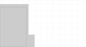
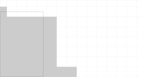
(a) Instant $t/t_{\mathrm{ref}}=0.44$	(b) Instant $t/t_{\mathrm{ref}}=1.1$
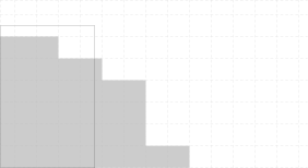
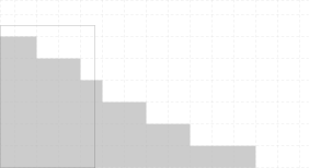
(c) Instant $t/t_{\mathrm{ref}}=2.2$	(d) Instant $t/t_{\mathrm{ref}}=5$

Figure 1: Graphical representation of the four frames in [23, Fig.2, p.685]. Gray boxes represent boxes that are completely or partially filled with sand; while white boxes represent empty boxes.

Let us now describe the approach we used to reproduce the above described physical experiment. Denote $p_{j}=([p_{j}]_{1},[p_{j}]_{2})^{T}\in\mathbb{R}^{2}$ for $j=1,\dots,n_{p}$, $p=(p_{1}^{T},\dots,p_{n_{p}}^{T})^{T}\in\mathbb{R}^{2n_{p}}$, and

$$\Psi_{x}(p)=x\left(\sum_{j=1}^{n_{p}}\sum_{i=j+1}^{n_{p}}\max\left\{0,(2r)^{2}-\|p_{j}-p_{i}\|_{2}^{2}\right\}^{2}\right)+(1-x)\sum_{j=1}^{n_{p}}[p_{j}]_{2},$$ (31)

where the “radius” $r>0$ and the “weight” $x\in(0,1)\subset\mathbb{R}$ are given constant. In this formulation, $n_{p}$ represents the number of balls, each $p_{j}\in\mathbb{R}^{2}$ ($j=1,\dots,n_{p}$) is the center of a ball, the first term in (31) (multiplied by $x$) forces the balls’ centers to be the “correct distance” apart; while the second term in (31) (multiplied by $1-x$) “pushes all the balls toward the ground”.

Consider the problem

$$\mbox{Minimize }\Psi_{x}(p_{1},\dots,p_{n_{p}})\mbox{ subject to }p\in D,$$ (32)

where $D=\{p\in\mathbb{R}^{2n_{p}}\;|\;p_{j}\geq 0\mbox{ for }j=1,\dots,n_{p}\}$. Independently of the value of $x\in(0,1)$, a solution to problem (32) consists in $n_{p}$ points representing the centers of $n_{p}$ non-overlapping identical balls with radius $r$ “resting on the floor” of the positive orthant of the two-dimensional Cartesian space. Thus, the dam collapse is modeled not just by changing $x$ but also by changing, simultaneously, the number of iterations of an optimization methods applied to (32) as we now describe.

Assume that $p^{0}\in D$ corresponds to the configuration represented in Figure 2. Given a maximum of iterations $y\in\mathbb{N}_{+}$, let $p^{0},p^{1},p^{2},\dots,p^{\bar{y}}\in D$ be the $\bar{y}\leq y$ iterates that result from the application of the Spectral Projected Gradient (SPG) method [13, 14, 15, 16] to problem (32) starting from $p^{0}$ and using as a stopping criteria a maximum of $y$ iterations or finding an iterate $p^{\bar{y}}$ such that

$$\|P_{D}(p^{\bar{y}}-\nabla\Psi_{x}(p^{\bar{y}}))-p^{\bar{y}}\|_{\infty}\leq\varepsilon_{\mathrm{opt}}^{\mathrm{spg}}:=10^{-8},$$

where $P_{D}$ represents the projector operator onto $D$. We aim to verify whether, by adjusting the weight $x$ in (31) and the maximum number of iterations $y$ of the SPG method, it is possible to construct a two-dimensional simulation of the dynamics of the dam-failure physical experiment through the iterates $p^{0},p^{1},p^{2},\dots,p^{\bar{y}}$.

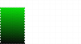
Figure 2: Initial guess $p^{0}$ for the SPG method.

We consider solving problem (32) with $r=0.125$ and $n_{p}=419$ using SPG with the initial guess $p^{0}$ depicted on Figure 1. We associate with the four frames depicted in Figures 1(a–d) binary matrices $M_{1},M_{2},M_{3},M_{4}\in\{0,1\}^{8\times 20}$ that represent whether there is sand in each box of the frame or not. In an analogous way, we define $M(p)\in\{0,1\}^{8\times 20}$ as the matrix associated with the point $p=(p_{1}^{T},\dots,p_{n_{p}}^{T})^{T}\in D\subset\mathbb{R}^{2n_{p}}$, that indicates whether each box contains at least a point $p_{j}$ or not. Given two $A=(a_{ij}),B=(b_{ij})\in\{0,1\}^{8\times 20}$, we also define the fitness function

$$\Pi(A,B)=\sum_{j=1}^{20}\sum_{i=1}^{8}|a_{ij}-b_{ij}|.$$

For a full sequence of iterates $p^{0},p^{1},p^{2},\dots,p^{\bar{y}}\in\Omega$ of the SPG method, that depends on the weight $x$ and the maximal number of iterations $y$, we define

$$f(x,y)=1-\frac{1}{640}\max_{c\geq 0}\left\{\sum_{\kappa=1}^{4}\Pi\left(M(p^{\lfloor c\,t_{\kappa}\rfloor}),M_{\kappa}\right)\right\},$$

where, if $\lfloor c\,t_{\kappa}\rfloor>\bar{y}$ and, thus, $p^{\lfloor c\,t_{\kappa}\rfloor}$ does not exist, then we consider $\Pi\left(M(p^{\lfloor c\,t_{\kappa}\rfloor}),M_{\kappa}\right)=0$. The value of $f$ can be computed by inspection of $c$. Finally, we define $h(y)=1/y$ and $\Omega=\{x\in\mathbb{R}\;|\;0\leq x\leq 1\}$.

We implemented Algorithm 7.1 in Fortran. In the numerical experiments, we considered, $\alpha=10^{-4}$, $\beta=100$, $\theta_{0}=0.5$, $\nu=2$, $r=2$, $p=2$, $\varepsilon_{\mathrm{feas}}=1/12{,}800$, $\varepsilon_{\mathrm{dist}}=10^{-4}$, and $\eta=10^{-6}$. In Algorithm 5.1, we considered $\sigma_{\min}=10^{-4}$ and $\gamma=10^{-4}$. The optimality condition of Algorithm 5.1 defined by $\eta$ is that the objective function to which this criterion is applied is not bigger, at the approximate optimizer $z$, than the values at the feasible points of the form $z\pm\eta$. The model $M(x_{k},x)$ is given by (30) with $k^{\prime}=\max\{0,k-1\}$. For the approximate minimization of the model we employ standard global one-dimensional search. As initial guess, we considered $(x_{0},y_{0})=(0.5,100)$. All tests were conducted on a computer with a 3.4 GHz Intel Core i5 processor and 8GB 1600 MHz DDR3 RAM memory, running macOS Mojave (version 10.14.6). Code was compiled by the GFortran compiler of GCC (version 8.2.0) with the -O3 optimization directive enabled. Table 1 shows the results; while Figure 3 illustrates de obtained solution. A rough comparison with Figure 9 of [23] indicates that our results are similar to the ones obtained by DEM-LBM and seem to be closer to the experimental results than the ones reported for MPM. As in the case of DEM-LBM and MPM, the discrepancies with respect to the experimental results are due to the behavior of the top part of the column. The whole process was completed in less than 1 minute of CPU time. The objective function equal to $1-618/640\approx 0.03$ at the final iterate means that at 97% of the “pixels” of the measured data matched the prediction of the model.

$k$	$x^{k}$	$y^{k}$	$f(x^{k},y^{k})$
0	0.5	100	$1-556/640$
1	0.9	200	$1-561/640$
2	0.99	400	$1-604/640$
3	0.99	800	$1-604/640$
4	0.999	1,600	$1-613/640$
5	0.99925	3,200	$1-617/640$
6	0.999275	6,400	$1-618/640$
7	0.999275	12,800	$1-618/640$

Table 1: Details of the application of Algorithm 7.1.

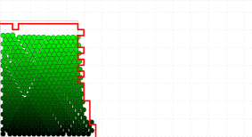
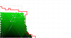
(a) $p^{384}$ associated with $t_{1}=0.44$	(b) $p^{961}$ associated with $t_{2}=1.1$
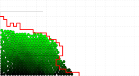
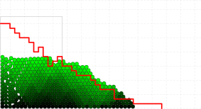
(c) $p^{1922}$ associated with $t_{3}=2.2$	(d) $p^{4369}$ associated with $t_{4}=5.0$

Figure 3: Graphical representation of $p^{384}$, $p^{961}$, $p^{1922}$, and $p^{4369}$ (corresponding to $c=873.2$) of a run of SPG with $x=0.999275$ and $y=12{,}800$. The red line is a rough representation of the physical experiment profile according to Fig. 2 of [23].

8 Final remarks

The application of Inexact Restoration to problems in which the objective function is evaluated inexactly has proved to be successful according to recent literature [9, 10, 42]. Real-life optimization problems use to be defined in domains more general than finite-dimensional Euclidean spaces, so that differentiability is out of question. The present paper aims to extend the established theory to this more general context. For this purpose, we found out that regularization-based algorithms are suitable for solving subproblems that arise in the Optimization Phase of IR. The regularization tools introduced in this paper are naturally inspired in the Euclidean case, as this is the environment in which regularization algorithms have been intensively developed in the last few years. In particular, we needed to introduce new optimality criteria and we emphasized the subtleties related with high-order models for minimization problems. We do not claim that the approach suggested in this paper for the Optimization Phase of IR is the definite word on this subject. In fact, much research is necessary to take advantage of the most reliable mathematical structures that are associated with real-life problems. Topological vector spaces should be considered in order to include problems in which the unknowns are generalized functions (distributions) and the topology is given by systems of semi-norms [17].

Many natural phenomena tend to converge to equilibrium states that are characterized as minimizers of “energy functions”. This is the reason why physical laws sometimes inspire optimization algorithms. For example, in [50] a method for solving nonlinear equations is linked to a system of second-order ordinary differential equations inspired in classical mechanics. In this paper, we suggested a movement in the opposite direction: Simulating a physical phenomenon by means of the behavior of an optimization algorithm. Of course this does not mean that physical events that are usually modelled by means of complex systems of differential equations may be always mimicked by the sequence of iterations of a simple minimization algorithm. However, the possibility that a minimization algorithm could give a first general approach to a complex phenomenon in which the basic principle is energy minimization cannot be excluded, especially when many physical parameters are unknown and, in practice, need to be estimated using available data.

We are optimistic that the techniques described in this paper may help understanding, describing and, at some point, predicting technological disasters due to dam breaking. Many qualitative and partially quantitative description of dam disasters exist in the scientific literature. For example, in [43] we find a useful report about the Brumadinho tailings dam disaster in Brazil in 2019. The paper contains many references about this event, other dam disasters, and the application of mathematical models to their analysis. See, for example, [47]. We plan to apply the techniques introduced in the present paper to the support of models of the Brumadinho event in the context of the activity of CRIAB (acronym for “Conflicts, Risks and Impacts Associated with Dams” in Portuguese), an interdisciplinary research group created at the University of Campinas for prediction and mitigation of the consequences of dam disasters.

References

- [1] R. Andreani, S. L. C. Castro, J. L. Chela, A. Friedlander, S. A. Santos, An inexact-restoration method for nonlinear bilevel programming problems, Computational Optimization and Applications 43, pp. 307–328, 2009.
- [2] M. B. Arouxét, N. E. Echebest, and E. A. Pilotta, Inexact Restoration method for nonlinear optimization without derivatives, Journal of Computational and Applied Mathematics 290, pp. 26–43, 2015.
- [3] N. Banihashemi and C. Y. Kaya, Inexact Restoration for Euler discretization of box-constrained optimal control problems, Journal of Optimization Theory and Applications 156, pp. 726–760, 2013.
- [4] N. Banihashemi and C. Y. Kaya, Inexact restoration and adaptive mesh refinement for optimal control, Journal of Industrial and Management Optimization 10, pp. 521–542, 2014.
- [5] S. Bellavia, G. Gurioli, B. Morini, and Ph.L. Toint, Adaptive regularization algorithms with inexact evaluations for nonconvex optimization, SIAM Journal on Optimization 29, pp. 2881–2915, 2019.
- [6] S. Bellavia, G. Gurioli, B. Morini, and Ph.L. Toint, High-order Evaluation Complexity of a Stochastic Adaptive Regularization Algorithm for Nonconvex Optimization Using Inexact Function Evaluations and Randomly Perturbed Derivatives, arXiv preprint arXiv:2005.04639, 2020.
- [7] S. Bellavia, N. Krejić, and B. Morini, Inexact restoration with subsampled trust‐region methods for finite‐sum minimization, Computational Optimization and Applications 76, pp. 701–736, 2020.
- [8] E. G. Birgin, L. F. Bueno, and J. M. Martínez, Assessing the reliability of general-purpose Inexact Restoration methods, Journal of Computational and Applied Mathematics 282, pp. 1–16, 2015.
- [9] E. G. Birgin, N. Krejić, and J. M. Martínez, On the employment of Inexact Restoration for the minimization of functions whose evaluation is subject to errors, Mathematics of Computation 87, pp. 1307–1326, 2018.
- [10] E. G. Birgin, N. Krejić, J. M. Martínez, Iteration and evaluation complexity on the minimization of functions whose computation is intrinsically inexact, Mathematics of Computation 89, pp. 253–278, 2020.
- [11] E. G. Birgin, R. D. Lobato, and J. M. Martínez, Constrained optimization with integer and continuous variables using inexact restoration and projected gradients, Bulletin of Computational Applied Mathematics 4, pp. 55–70, 2016.
- [12] E. G. Birgin and J. M. Martínez, Local convergence of an Inexact-Restoration method and numerical experiments, Journal of Optimization Theory and Applications 127, pp. 229–247, 2005.
- [13] E. G. Birgin, J. M. Martínez, and M. Raydan. Nonmonotone spectral projected gradient methods on convex sets. SIAM Journal on Optimization 10, pp. 1196–1211, 2000.
- [14] E. G. Birgin, J. M. Martínez, and M. Raydan, Algorithm 813: SPG – software for convex-constrained optimization, ACM Transactions on Mathematical Software 27, pp. 340–349, 2001.
- [15] E. G. Birgin, J. M. Martínez and M. Raydan, Inexact Spectral Projected Gradient methods on convex sets, IMA Journal of Numerical Analysis 23, pp. 539–559, 2003.
- [16] E. G. Birgin, J. M. Martínez, and M. Raydan, Spectral Projected Gradient Methods: Review and Perspectives, Journal of Statistical Software 60, issue 3, 2014.
- [17] N. Bourbaki, Elements of Mathematics — Topological Vector Spaces, Chapters 1–5, Springer, 2003.
- [18] L. F. Bueno, A. Friedlander, J. M. Martínez, and F. N. C. Sobral, Inexact Restoration method for derivative-free optimization with smooth constraints, SIAM Journal on Optimization 23, pp. 1189–1231, 2013.
- [19] L. F. Bueno, G. Haeser, and J. M. Martínez, A flexible Inexact-Restoration method for constrained optimization, Journal of Optimization Theory and Applications 165, pp. 188–208, 2015.
- [20] L. F. Bueno, G. Haeser, and J. M. Martínez, An inexact restoration approach to optimization problems with multiobjective constraints under weighted-sum scalarization, Optimization Letters 10, pp. 1315–1325, 2016.
- [21] L. F. Bueno and J. M. Martínez, On the complexity of an Inexact Restoration method for constrained optimization, SIAM Journal on Optimization 30, pp. 80–101, 2020.
- [22] R. G. Carter, Numerical experience with a class of algorithms for nonlinear optimization using inexact function and gradient information, SIAM Journal on Scientific Computing 14, pp. 368–388, 1993.
- [23] F. Ceccato, A. Leonardi, V. Girardi, P. Simonini, and M. Pirulli, Numerical and experimental investigation of saturated granular column collapse in air, Soils and Foundations 60, pp. 683–696, 2020.
- [24] A. R. Conn, N. I. M. Gould, and Ph. L. Toint, Trust Region Methods, MPS SIAM Series in Optimization, Philadelphia, 2000.
- [25] N. Echebest, M. L. Schuverdt, and R. P. Vignau, An inexact restoration derivative-free filter method for nonlinear programming, Computational and Applied Mathematics 36, pp. 693–718, 2017.
- [26] D. Fernández, E. A. Pilotta, and G. A. Torres, An inexact restoration strategy for the globalization of the sSQP method, Computational Optimization and Applications 54, pp. 595–617, 2013.
- [27] P. S. Ferreira, E. W. Karas, M. Sachine, F. N. C. Sobral, Global convergence of a derivative-free inexact restoration filter algorithm for nonlinear programming, Optimization 66, pp. 271–292, 2017.
- [28] A. Fischer and A. Friedlander, A new line search inexact restoration approach for nonlinear programming, Computational Optimization and Applications 46, pp. 336–346, 2010.
- [29] J. B. Francisco, D. S. Gonçalves, F. S. V. Bazán, and L. L. T. Paredes, Non-monotone inexact restoration method for nonlinear programming, Computational Optimization and Applications 76, pp. 867–888, 2020.
- [30] J. B. Francisco, D. S. Gonçalves, F. S. V. Bazán, and L. L. T. Paredes, Nonmonotone inexact restoration approach for minimization with orthogonality constraints, Numerical Algorithms 86, pp. 1651–1684, 2021.
- [31] J. B. Francisco, J. M. Martínez, L. Martínez, and F. Pisnitchenko, Inexact restoration method for minimization problems arising in electronic structure calculations, Computational Optimization and Applications 50, pp. 555–590, 2011.
- [32] M. A. Gomes-Ruggiero, J. M. Martínez, and S. A. Santos, Spectral Projected Gradient method with Inexact Restoration for minimization with nonconvex constraints, SIAM Journal on Scientific Computing 31, pp. 1628–1652, 2009.
- [33] S. Gratton, E. Simon, D. Titley-Peloquin, Ph. L. Toint, Minimizing convex quadratics with variable precision conjugate gradients, Numerical Linear Algebra with Applications 28, e2337, 2021.
- [34] S. Gratton, E. Simon, and Ph. L. Toint, An algorithm for the minimization of nonsmooth nonconvex functions using inexact evaluations and its worst-case complexity, Mathematical Programming 187, 1–24, 2021.
- [35] S. Gratton and Ph. L. Toint, A note on solving nonlinear optimization problems in variable precision, Computational Optimization and Applications 76, pp. 917–933, 2020.
- [36] E. Karas, E. A. Pilotta, and A. Ribeiro, Numerical comparison of merit function with filter criterion in Inexact Restoration algorithms using hard-spheres problems, Computational Optimization and Applications 44, pp. 427–441, 2009.
- [37] C. Y. Kaya, Inexact Restoration for Runge–Kutta discretization of optimal control problems, SIAM Journal on Numerical Analysis 48, pp. 1492–1517, 2010.
- [38] C. Y. Kaya and J. M. Martínez, Euler discretization and Inexact Restoration for optimal control, Journal of Optimization Theory and Applications 134, pp. 191–206, 2007.
- [39] T. G. Kolda, R. M. Lewis, and V. Torczon, Optimization by direct search: new perspectives on some classical and modern methods, SIAM Review 45, pp. 385–482, 2003.
- [40] T. G. Kolda, R. M. Lewis, and V. Torczon, Stationarity results for generating set search for linearly constrained optimization, SIAM Journal on Optimization 17, pp. 943–968, 2006.
- [41] D. P. Kouri, M. Heinkenschloss, D. Ridzal, and B. G. van Bloemen Waanders, Inexact objective function evaluations in a trust-region algorithm for PDE-constrained optimization under uncertainty, SIAM Journal on Scientific Computing 36, pp. A3011–A3029, 2014.
- [42] N. Krejić and J. M. Martínez, Inexact Restoration approach for minimization with inexact evaluation of the objective function, Mathematics of Computation 85, pp. 1775–1791, 2016.
- [43] R. E. de Lima, J. L. Picanço, A. F. da Silva, and F. A. Acordes, An anthropogenic flow type gravitational mass movement: the Córrego de Feijão tailings dam disaster, Brumadinho, Brazil, Landslides 17, pp. 2895–2906, 2020.
- [44] J. M. Martínez, Inexact-restoration method with Lagrangian tangent decrease and new merit function for nonlinear programming, Journal of Optimization Theory and Applications 111, 39–58, 2001.
- [45] J.M. Martínez and E. A. Pilotta, Inexact restoration algorithms for constrained optimization, Journal of Optimization Theory and Applications 104, pp. 135–163, 2000.
- [46] J. M. Martínez and E. A. Pilotta, Inexact restoration methods for nonlinear programming: advances and perspectives, in L. Qi, K. Teo, X. Yang (eds.), Optimization and Control with Applications, Applied Optimization 96, Springer, New York, NY, 2005, pp. 271–291.
- [47] M. Pirulli, M. Barbero, M. Martinelli, M. Marchelli, and C. Scavia, The failure of the Stava Valley tailings dam (Northern Italy): numerical analysis of the flow dynamics and rheological properties, Geoenvironmental Disasters 4, article number 3, 2017.
- [48] C. E. P. Silva and M. T. T. Monteiro, A filter inexact-restoration method for nonlinear programming, TOP 16, pp. 126–146, 2008.
- [49] J. Walpen, P. A. Lotito, E. M. Mancinelli, and L. Parente, The demand adjustment problem via inexact restoration method, Computational and Applied Mathematics 39, article number 204, 2020.
- [50] F. Zirilli, The solution of nonlinear systems of equations by second order systems of O.D.E. and linearly implicit A-stable techniques, SIAM Journal on Numerical Analysis 19, pp. 800–815, 1982.