Mid-Air Drawing of Curves on 3D Surfaces in Virtual Reality

Abstract.

Complex 3D curves can be created by directly drawing mid-air in immersive environments (Augmented and Virtual Realities). Drawing mid-air strokes precisely on the surface of a 3D virtual object, however, is difficult; necessitating a projection of the mid-air stroke onto the user “intended” surface curve. We present the first detailed investigation of the fundamental problem of 3D stroke projection in VR. An assessment of the design requirements of real-time drawing of curves on 3D objects in VR is followed by the definition and classification of multiple techniques for 3D stroke projection. We analyze the advantages and shortcomings of these approaches both theoretically and via practical pilot testing. We then formally evaluate the two most promising techniques spraycan and mimicry with 20 users in VR. The study shows a strong qualitative and quantitative user preference for our novel stroke mimicry projection algorithm. We further illustrate the effectiveness and utility of stroke mimicry, to draw complex 3D curves on surfaces for various artistic and functional design applications.

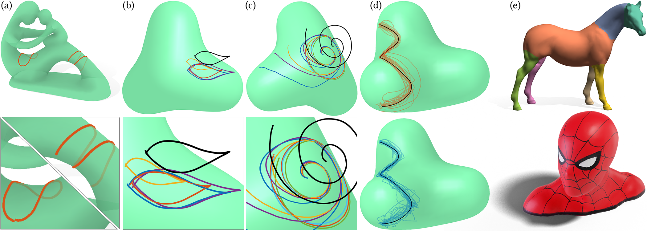
Figure 1. Drawing curves mid-air that lie precisely on the surface of a virtual 3D object in AR/VR is difficult (a). Projecting mid-air 3D strokes (black) onto 3D objects is an under-constrained problem with many seemingly reasonable solutions (b). We analyze this fundamental AR/VR problem of 3D stroke projection, define and characterize multiple novel projection techniques (c), and test the two most promising approaches—spraycan shown in blue and mimicry shown in red in (b)–(d)—using a quantitative study with 20 users (d). The user-preferred mimicry technique attempts to mimic the 3D mid-air stroke as closely as possible when projecting onto the virtual object. We showcase the importance of drawing curves on 3D surfaces, and the utility of our novel mimicry approach, using multiple artistic and functional applications (e) such as interactive shape segmentation (top) and texture painting (bottom).

1. Introduction

Drawing is a fundamental tool of human visual expression and communication. Digital sketching with pens, styli, mice, and even fingers in 2D is ubiquitous in visually creative computing applications. Drawing or painting on 3D virtual objects for example, is critical to interactive 3D modelling, animation, and visualization, where its uses include: object selection, annotation, and segmentation [Heckel et al., 2013; Meng et al., 2011; Jung et al., 2002]; 3D curve and surface design [Igarashi et al., 1999; Nealen et al., 2007]; strokes for 3D model texturing or painterly rendering [Kalnins et al., 2002] (Figure 1e). In 2D, digitally drawn on-screen strokes are WYSIWYG mapped onto 3D virtual objects, by projecting 2D stroke points through the given view onto the virtual object(s) (Figure 2a).

Sketching in immersive environments (AR/VR) has the mystical aura of a magical wand, allowing users to draw directly in 3D. Mid-air drawing has the potential to significantly disrupt interactive 3D graphics, as evidenced by the increasing popularity of applications such as Tilt Brush [Google, 2020] and Quill [Oculus, 2020]. A fundamental requirement for numerous interactive 3D applications in AR/VR is the ability to directly draw, or project drawn 3D strokes, precisely on virtual objects. While directly drawing on a physical object is reasonably easy, drawing directly on a virtual 3D object is near impossible without haptic constraints (Figure 3). Furthermore, unlike 2D drawing, where the WYSIWYG view-based projection of 2D strokes onto 3D objects is unambiguously clear, the user-intended mapping of a mid-air 3D stroke onto a 3D object is less obvious. We present the first detailed investigation into plausible user-intended projections of mid-air strokes on to 3D virtual objects.

Interfaces for 2D/3D curve creation in general, use perceptual insights or geometric assumptions like smoothness and planarity, to project, neaten, or otherwise process sketched strokes. Some applications wait for user stroke completion before processing it in entirety, for example when fitting splines [Bae et al., 2008]. Our goal is to establish an application agnostic, base-line projection approach for mid-air 3D strokes. We thus assume a stroke is processed while being drawn and inked in real-time, i.e., the output curve corresponding to a partially drawn stroke is fixed/inked in real-time, based on partial stroke input [Thiel et al., 2011].

One might further conjecture that all “reasonable” and mostly continuous projections would produce similar results, as long as users are given interactive visual feedback of the projection. This is indeed true for tasks requiring discrete point-on-surface selection, where users can freely re-position the drawing tool until its interactively visible projection corresponds to user-intent. Real-time curve drawing, however, is very sensitive to the projection technique, where any mismatch between user intention and algorithmic projection, is continuously inked into the projected curve (Figure 1d).

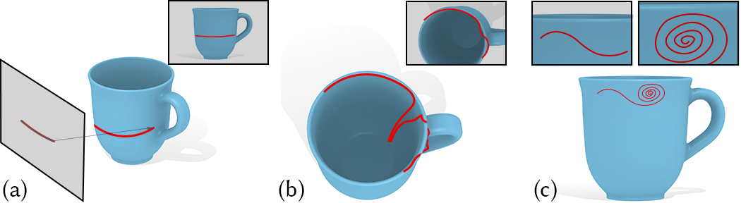
Figure 2. Stroke projection using a 2D interface is typically WYSIWYG: 2D points along a user stroke (a, inset) are ray-cast through the given view to create corresponding 3D curve points on the surface of 3D scene objects (a). Even small errors or noise in 2D strokes can cause large discontinuities in 3D, especially near ridges and sharp features (b). Complex curves spanning many viewpoints, or with large scale variations in detail, often require the curve to be drawn in segments from multiple user-adjusted viewpoints (c).

2D Strokes Projected onto 3D Objects

The standard user-intended mapping of a 2D on-screen stroke is a raycast projection through the given monocular viewpoint. Raycasting is WYSIWYG (What You See Is What You Get): the 3D curve visually matches the 2D stroke from said viewpoint (Figure 2a). Ongoing research on mapping 2D strokes to 3D objects assumes this fundamental view-centric projection, focusing instead on specific problems such as creating curves around ridge/valley features (where small 2D error can cause large 3D depth error, Figure 2b); or drawing complex curves with large scale variation (where multiple viewpoint changes are needed while drawing, Figure 2c). These problems are mitigated by the direct 3D input and viewing flexibility of AR/VR, assuming the mid-air stroke to 3D object projection matches user intent.

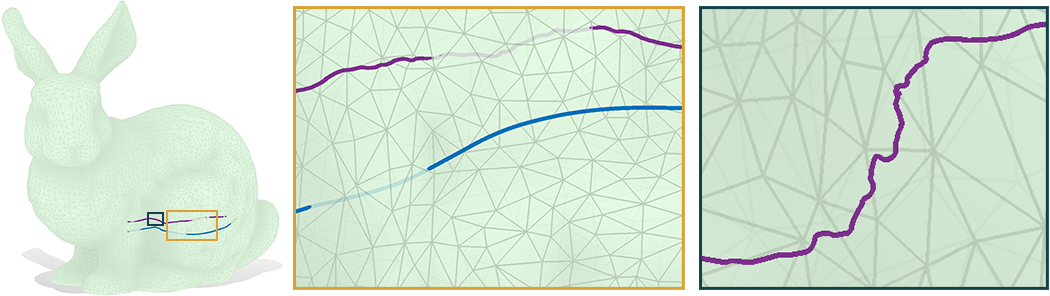
Figure 3. Mid-air drawing precisely on a 3D virtual object is difficult (faint regions of strokes are behind the surface), regardless of drawing quick smooth strokes (blue), or slow detailed strokes (purple). Deliberately slow drawing is further detrimental to stroke aesthetic (right).

3D Strokes Projected onto 3D Objects

Physical analogies motivate existing approaches to defining a user-intended projection from 3D points in a mid-air stroke to 3D points on a virtual object (Figure 4). Graffiti-style painting with a spraycan is arguably the current standard, deployed in commercial immersive paint and sculpt software such as Medium [Adobe, 2021] and Gravity Sketch [2020]. A closest-point projection approximates drawing with the tool on the 3D object, without actual physical contact (used by the ”guides” tool in Tilt Brush [Google, 2020]). Like view-centric 2D stroke projection, these approaches are context-free: processing each mid-air point independently. The AR/VR drawing environment comprising six–degree of freedom controller input and unconstrained binocular viewing, is however, significantly richer than 2D sketching. The user-intended projection of a mid-air stroke (§ 3) as a result is complex, influenced by the ever-changing 3D relationship between the view, drawing controller and virtual object. We therefore argue the need for historical context (i.e., the partially drawn stroke and its projection) in determining the projection of a given stroke point. We balance the use of this historical context, with the overarching goal of a general purpose projection that makes little or no assumption on the nature of the user stroke or its projection.

We thus explore anchored projection techniques, that minimally use the most recently projected stroke point, as context for projecting the current stroke point (§ 4). We evaluate various anchored projections, both theoretically and practically by pilot testing. Our most promising and novel approach anchored-smooth-closest-point (also called mimicry), captures the natural tendency of a user stroke to mimic the shape of the desired projected curve. A formal user study in VR (§ 5) shows mimicry to perform significantly better than spraycan (the current baseline) in producing curves that match user intent (§ 6). While our formal evaluation is limited to VR, the fundamental problem we study could directly translate to AR scenarios as well. This paper thus contributes, to the best of our knowledge, the first principled investigation of real-time inked techniques to project 3D mid-air strokes drawn in VR onto 3D virtual objects, and a novel stroke projection benchmark for VR: mimicry.

2. Related Work

Our work is related to research on drawing and sculpting in immersive realities, interfaces for drawing curves on, near, and around surfaces, and sketch-based modelling tools.

2.1. Immersive Sketching and Modelling

Immersive creation has a long history in computer graphics. Immersive 3D sketching was pioneered by the HoloSketch system [Deering, 1995], which used a 6-DoF wand as the input device for creating polyline sketches, 3D tubes, and primitives. In a similar vein, various subsequent systems have explored the creation of freeform 3D curves and swept surfaces [Schkolne et al., 2001; Keefe et al., 2001; Google, 2020]. While directly turning 3D input to creative output is acceptable for ideation, the inherent imprecision of 3D sketching is quickly apparent when more structured creation is desired.

The perceptual and ergonomic challenges in precise control of 3D input is well-known [Keefe et al., 2007; Wiese et al., 2010; Arora et al., 2017; Machuca et al., 2019; Machuca et al., 2018], resulting in various methods for correcting 3D input. Input 3D curves have been algorithmically regularized to snap onto existing geometry, as with the FreeDrawer [Wesche and Seidel, 2001] system, or constrained physically to 2D input with additional techniques for “lifting” these curves into 3D [Jackson and Keefe, 2016; Arora et al., 2018; Kwan and Fu, 2019; Paczkowski et al., 2011]. Haptic rendering devices [Keefe et al., 2007; Kamuro et al., 2011] and tools utilizing passive physical feedback [Grossman et al., 2002] are an alternate approach to tackling the imprecision of 3D inputs. We are motivated by similar considerations.

Arora et al. [2017] demonstrated the difficulty of creating curves that lie exactly on virtual surfaces in VR, even when the virtual surface is a plane. This observation directly motivates our exploration of techniques for projecting 3D strokes onto surfaces, instead of coercing users to awkwardly draw exactly on a virtual surface.

2.2. Drawing Curves on, near, and around Surfaces

Curve creation and editing on or near the surface of 3D virtual objects is fundamental for a variety of artistic and functional shape modelling tasks. Functionally, curves on 3D surfaces are used to model or annotate structural features [Gal et al., 2009; Stanculescu et al., 2013], define trims and holes [Schmidt and Singh, 2010], and to provide handles for shape deformation [Singh and Fiume, 1998; Kara and Shimada, 2007; Nealen et al., 2007], registration [Gehre et al., 2018] and remeshing [Krishnamurthy and Levoy, 1996; Takayama et al., 2013]. Artistically, curves on surfaces are used in painterly rendering [Gooch and Gooch, 2001], decal creation [Schmidt et al., 2006], texture painting [Adobe, 2020], and even texture synthesis [Fisher et al., 2007]. Curve on surface creation in this body of research typically uses the established view-centric WYSIWYG projection of on-screen sketched 2D strokes. While the sketch view-point in these interfaces is interactively set by the user, there has been some effort in automatic camera control for drawing [Ortega and Vincent, 2014], auto-rotation of the sketching view for 3D planar curves [McCrae et al., 2014], and user assistance in selecting the most sketchable viewpoints [Bae et al., 2008]. Immersive 3D drawing enables direct, view-point independent 3D curve sketching, and is thus an appealing alternative to these 2D interfaces.

Our work is also related to drawing curves around surfaces. Such techniques are important for a variety of applications: modelling string and wire that wrap around objects [Coleman and Singh, 2006]; curves that loosely conform to virtual objects [Krs et al., 2017]; clothing design on a 3D mannequin [Turquin et al., 2007]; layered modelling of shells and armour [De Paoli and Singh, 2015]; and the design and grooming of hair and fur [Fu et al., 2007; Schmid et al., 2011; Xing et al., 2019]. Some approaches such as SecondSkin [De Paoli and Singh, 2015] and Skippy [Krs et al., 2017] use insights into spatial relationship between a 2D stroke and the 3D object, to infer a 3D curve that lies on and around the surface of the object. Other techniques like Cords [Coleman and Singh, 2006] or hair and clothing design [Xing et al., 2019] are closer to our work, in that they drape 3D curve input on and around 3D objects using geometric collisions or physical simulation. In contrast, this paper is focused on the general problem of projecting a drawn 3D stroke to a real-time inked curve on the surface of a 3D object. While we do not address curve creation with specific geometric relationships to the object surface (like distance-offset curve), our techniques can be extended to incorporate geometry-specific terms (§ 8).

2.3. Sketch-based 3D Modelling

Sketch-based 3D modelling is a rich ongoing area of research (see survey by Olsen et al. [2009]). Typically, these systems interpret 2D sketch inputs for various shape modelling tasks. One could categorize these modelling approaches as single-view (akin to traditional pen on paper) [Schmidt et al., 2009; Andre and Saito, 2011; Chen et al., 2013; Xu et al., 2014] or multi-view (akin to 3D modelling with frequent view manipulation) [Igarashi et al., 1999; Fan et al., 2004; Nealen et al., 2007; Bae et al., 2008; Fan et al., 2013]. Single-view techniques use perceptual insights and geometric properties of the 2D sketch to infer its depth in 3D, while multi-view techniques explicitly use view manipulation to specify 3D curve attributes from different views. While our work utilizes mid-air 3D stroke input, the ambiguity of projection onto surfaces connects it to the interpretative algorithms designed for sketch-based 3D modelling. We aim to take advantage of the immersive interaction space by allowing view manipulation as and when desired, independent of geometry creation.

3. Projecting Strokes on 3D Objects

We first formally state the problem of projecting a mid-air 3D stroke onto a 3D virtual object. Let $\mathcal{M}=(V,E,F)$ be a 3D object, represented as a manifold triangle mesh embedded in $\mathbb{R}^{3}$. A user draws a piece-wise linear mid-air stroke by moving a 6-DoF controller or drawing tool in VR. The 3D stroke $\mathcal{P}\subset\mathbb{R}^{3}$ is a sequence of $n$ points $(\mathbf{p}_{i})_{i=0}^{n-1}$, connected by line segments. Corresponding to each point $\mathbf{p}_{i}\in\mathbb{R}^{3}$, is a system state $S_{i}=(\mathbf{h}_{i},\mathbf{c}_{i},\mathsf{h}_{i},\mathsf{c}_{i})$, where $\mathbf{h}_{i},\mathbf{c}_{i}\in\mathbb{R}^{3}$ are the positions of the headset and the controller, respectively, and $\mathsf{h}_{i},\mathsf{c}_{i}\in Sp(1)$ are their respective orientations, represented as unit quaternions. Also, without loss of generality, assume $\mathbf{c}_{i}=\mathbf{p}_{i}$, i.e. the controller positions describe the stroke points $\mathbf{p}_{i}$.

We want to define a projection $\pi$, which transforms the sequence of points $(\mathbf{p}_{i})_{i=0}^{n-1}$ to a corresponding sequence of points $(\mathbf{q}_{i})_{i=0}^{n-1}$ on the 3D virtual object, i.e. $\mathbf{q}_{i}\in\mathcal{M}$. Consecutive points in this sequence are connected by geodesics on $\mathcal{M}$, describing the projected curve $\mathcal{Q}\subset\mathcal{M}$. The aim of a successful projection method of course, is to match the undisclosed user-intended curve. The projection is also designed for real-time inking of curves: points $\mathbf{p}_{i}$ are processed upon input and projected in real-time (under 100ms) to $\mathbf{q}_{i}$ using the current system state $S_{i}$, and optionally, prior system states $(S_{j})_{j=0}^{i-1}$, stroke points $(\mathbf{p}_{j})_{j=0}^{i-1}$ and projections $(\mathbf{q}_{j})_{j=0}^{i-1}$.

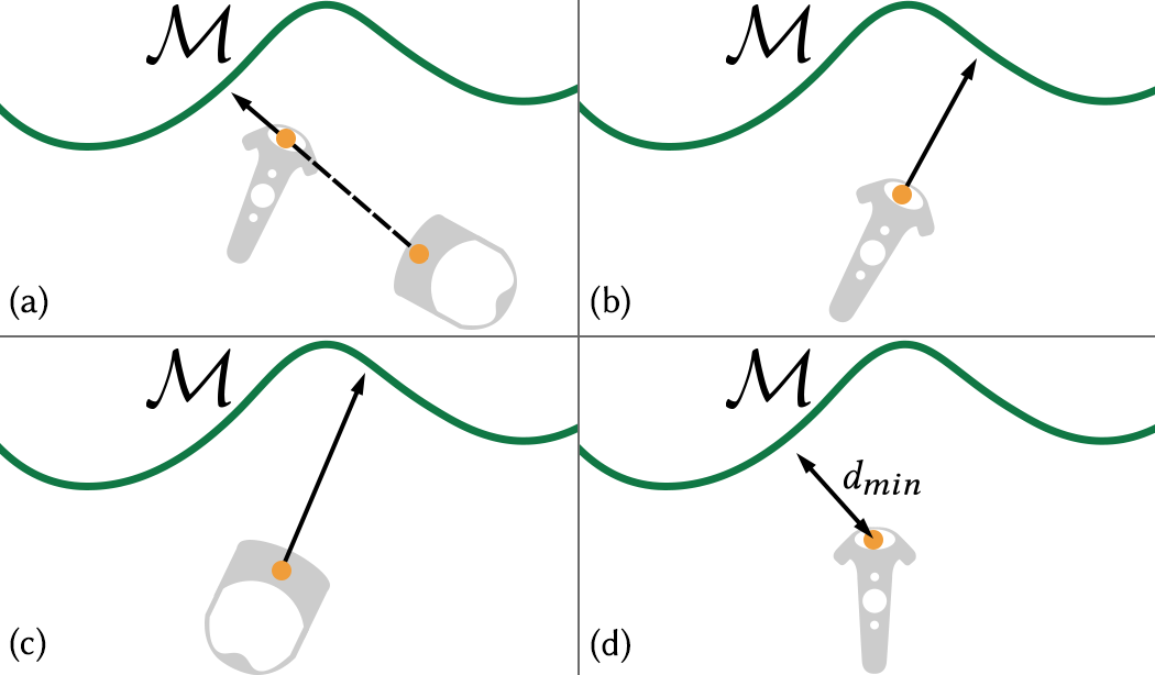
Figure 4. Context-free techniques: occlude projects points from the controller origin along the direction from the eye (HMD origin) to the controller (a); spraycan projects points from the controller origin in a direction defined by the controller’s orientation (b); head-centric, akin to 2D projects points along the view direction defined by HMD orientation (c); snap projects points from the controller origin to their closest-point on $\mathcal{M}$ (d).

3.1. Context-Free Projection Techniques

Context-free techniques project points independent of each other, simply based on the spatial relationships between the controller, HMD, and 3D object ( Figure 4). We can further categorize techniques as raycast or proximity based.

3.1.1. Raycast Projections

View-centric projection in 2D interfaces projects points from the screen along a ray from the eye through the screen point, to where the ray first intersects the 3D object. In an immersive setting, raycast approaches similarly use a ray emanating from the 3D stroke point to intersect 3D objects. This ray $(\mathbf{o},\mathbf{d})$ with origin $\mathbf{o}$ and direction $\mathbf{d}$ can be defined in a number of ways. Similar to pointing behaviour, occlude defines this ray from the eye through the controller origin (Figure 4a) $\left(\mathbf{c}_{i},(\mathbf{c}_{i}-\mathbf{h}_{i})/\|\mathbf{c}_{i}-\mathbf{h}_{i}\|\right)$. If the ray intersects $\mathcal{M}$, then the closest intersection to $\mathbf{p}_{i}$ defines $\mathbf{q}_{i}$. In case of no intersection, $\mathbf{p}_{i}$ is ignored in defining the projected curve, i.e., $\mathbf{q}_{i}$ is marked undefined and the projected curve connects $\mathbf{q}_{i-1}$ to $\mathbf{q}_{i+1}$ (or the proximal index points on either side of $i$ for which projections are defined). The spraycan approach treats the controller like a spraycan, defining the ray like a nozzle direction in the local space of the controller (Figure 4b). For example the ray could be defined as $(\mathbf{c}_{i},\mathbf{f}_{i})$, where the nozzle $\mathbf{f}_{i}=\mathsf{c}_{i}\cdot[0,0,1]^{T}$ is the controller’s local z-axis (or forward direction). Alternately, head-centric projection can define the ray using the HMD’s view direction as $(\mathbf{h}_{i},\mathsf{h}_{i}\cdot[0,0,1]^{T})$ (Figure 4c).

Pros and Cons: The strengths of raycasting are: a predictable visual/proprioceptive sense of ray direction; a spatially continuous mapping between user input and projection rays; and scenarios where it is difficult or undesirable to reach and draw close to the virtual object. Its biggest limitation stems from the controller/HMD-based ray direction being completely agnostic of the shape or location of the 3D object. Projected curves can consequently be very different in shape and size from drawn strokes (Figure 5a–b), and ill-defined for stroke points with no ray-object intersection.

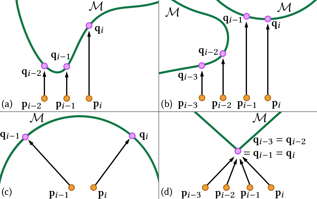
Figure 5. Context-free projection problems: large depth disparity (a), unexpected jumps (b), projection discontinuities (c), and undesirable snapping (d).

3.1.2. Proximity-Based Projections

In 2D interfaces, the on-screen 2D strokes are typically distant to the viewed 3D scene, necessitating some form of raycast projection onto the visible surface of 3D objects. In AR/VR, however, users are able to reach out in 3D and directly draw the desired curve on the 3D object. While precise mid-air drawing on a virtual surface is very difficult in practice (Figure 3), projection methods based on proximity between the mid-air stroke and the 3D object are certainly worth investigation.

The simplest proximity-based projection technique snap, projects a stroke point $\mathbf{p}_{i}$ to its closest-point in $\mathcal{M}$ (Figure 4d).

(1) $$\mathbf{q}_{i}=\pi_{snap}(\mathbf{p}_{i})=\operatorname*{arg\,min}_{\mathbf{x}\in\mathcal{M}}\ d(\mathbf{p}_{i},\mathbf{x}),$$

where $d(\cdot,\cdot)$ is the Euclidean distance between two points. Unfortunately, for triangle meshes, closest-point projection tends to snap to mesh edges (blue curve inset), resulting in unexpectedly jaggy projected curves, even for smooth 3D input strokes (black curve inset) [Panozzo et al., 2013]. These discontinuities are due to the discrete nature of the mesh representation, as well as spatial singularities in closest point computation even for smooth 3D objects. We mitigate this problem by formulating an extension of Panozzo et al.’s Phong projection [2013] in § 3.2, that simulates projection onto an imaginary smooth surface approximated by the mesh. We denote this smooth-closest-point projection as $\pi_{SCP}$ (red curve inset).

Pros and Cons: The biggest strength of proximity-based projection is it exploits the immersive concept of drawing directly on or near an object, using the spatial relationship between a 3D stroke point and the 3D object to determine projection. The main limitation is that since users rarely draw precisely on the surface, discontinuities in concave regions (Figure 5c) and undesirable snapping in highly-convex regions (Figure 5d) persist when projecting distantly drawn stoke points, even when using smooth-closest-point. In § 4.1, we address this problem using stroke mimicry to anchor distant stroke points close to the object to be finally projected using smooth-closest-point.

3.2. Smooth-Closest-Point Projection

(a) Computing weighted averages in Panozzo et al. [2013].

(b) Computing smooth-closest-point projection.

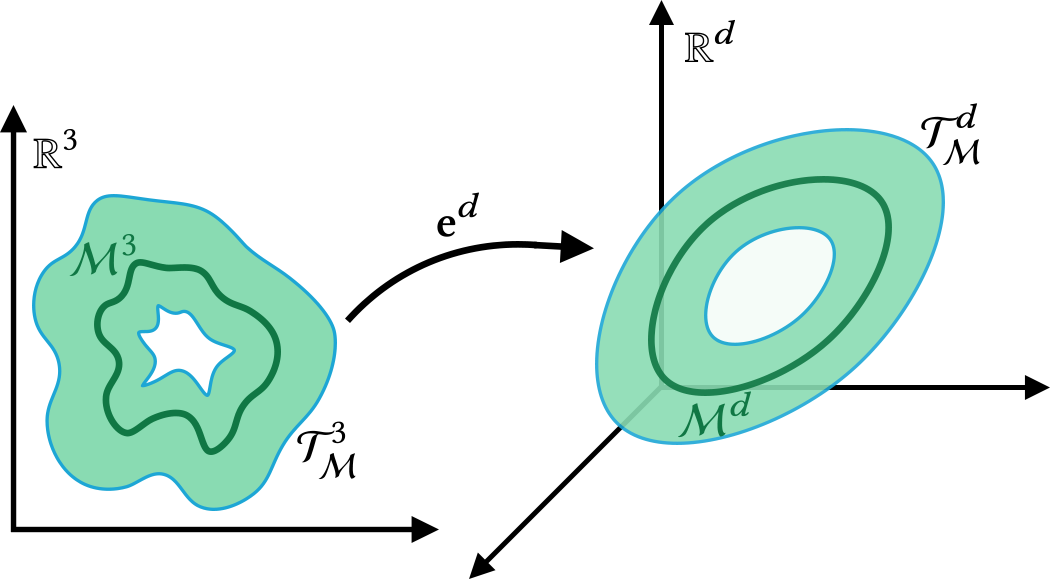
(c) Computing a $d$-dimensional embedding for $\mathcal{M}$ and $\mathcal{T}_{\mathcal{M}}$.

Figure 6. Panozzo et al. [2013] compute weighted averages on surfaces (a), while we want to compute a smooth closest-point projection for an arbitrary point near the mesh in $\mathbb{R}^{3}$ (b). We therefore embed $\mathcal{T}_{\mathcal{M}}$—the region around the mesh—in higher-dimensional space $\mathbb{R}^{d}$, instead of just $\mathcal{M}$ (c).

Our goal with smooth-closest-point projection is to define a mapping from a 3D point to a point on $\mathcal{M}$ that approximates the closest point projection but tends to be functionally smooth, at least for points near the 3D object. We note that computing the closest point to a Laplacian-smoothed mesh proxy, for example, will also provide a smoother mapping than $\pi_{snap}$, but a potentially poor closest-point approximation to the original mesh.

Phong projection, introduced by Panozzo et al. [2013], addresses these goals for points expressible as weighted-averages of points on $\mathcal{M}$, but we extend their technique to define a smooth-closest-point projection for points in the neighbourhood of the mesh. For completeness, we first present a brief overview of their technique.

Phong projection is a two-step approach to map a point $\mathbf{y}^{3}\in\mathbb{R}^{3}$ to a manifold triangle mesh $\mathcal{M}$ embedded in $\mathbb{R}^{3}$, emulating closest-point projection on a smooth surface approximated by the triangle mesh. First, $\mathcal{M}$ is embedded in a higher dimensional Euclidean space $\mathbb{R}^{d}$ such that Euclidean distance (between points on the mesh) in $\mathbb{R}^{d}$ approximates geodesic distances in $\mathbb{R}^{3}$. Second, analogous to vertex normal interpolation in Phong shading, a smooth surface is approximated by blending tangent planes across edges. Barycentric coordinates at a point within a triangle are used to blend the tangent planes corresponding to the three edges incident to the triangle. We extend the first step to a higher dimensional embedding of not just the triangle mesh $\mathcal{M}$, but a tetrahedral mesh of an offset volume around the mesh $\mathcal{M}$ (Figure 6). The second step remains the same, and we refer the reader to Panozzo et al. [2013] for details. Such offset volumes, or shells, around triangle meshes have also been utilized in recent methods for curve design [Jin et al., 2019] and for attribute transfer between similar triangle meshes [Jiang et al., 2020].

For clarity, we refer to $\mathcal{M}$ embedded in $\mathbb{R}^{3}$ as $\mathcal{M}^{3}$, and the embedding in $\mathbb{R}^{d}$ as $\mathcal{M}^{d}$. Panozzo et al. compute $\mathcal{M}^{d}$ by first embedding a subset of the vertices in $\mathbb{R}^{D}$ using metric multi-dimensional scaling (MDS) [Cox and Cox, 2008], aiming to preserve the geodesic distance between the vertices. The embedding of the remaining vertices is then computed using LS-meshes [Sorkine and Cohen-Or, 2004].

For the problem of computing weighted averages on surfaces, one only needs to project 3D points of the form $\mathbf{y}^{3}=\sum w_{i}\mathbf{x}_{i}^{3}$, where all $\mathbf{x}_{i}^{3}\in\mathcal{M}^{3}$. The point $\mathbf{y}^{3}$ is lifted into $\mathbb{R}^{d}$ by simply defining $\mathbf{y}^{d}=\sum w_{i}\mathbf{x}_{i}^{d}$, where $\mathbf{x}_{i}^{d}$ is defined as the point on $\mathcal{M}^{d}$ with the same implicit coordinates (triangle and barycentric coordinates) as $\mathbf{x}_{i}^{3}$ does on $\mathcal{M}^{3}$. Therefore, their approach only embeds $\mathcal{M}$ into $\mathbb{R}^{d}$ (Figure 6a,c). In contrast, we want to project arbitrary points near $\mathcal{M}^{3}$ onto it using the Phong projection. Therefore, we compute the offset surfaces at signed-distance $\pm\mu$ from $\mathcal{M}$. We then compute a tetrahedral mesh $\mathcal{T}_{\mathcal{M}}^{3}$ of the space between these two surfaces in $\mathbb{R}^{3}$. In the final precomputation step, we embed the vertices of $\mathcal{T}_{\mathcal{M}}$ in $\mathbb{R}^{d}$ using MDS and LS-Meshes as described above.

Now, given a 3D point $\mathbf{y}^{3}$ within a distance $\mu$ from $\mathcal{M}^{3}$, we situate it within $\mathcal{T}_{\mathcal{M}}^{3}$, use tetrahedral Barycentric coordinates to infer its location in $\mathbb{R}^{d}$, and then compute its Phong projection (Figure 6b,c). We fallback to closest-point projection for points outside $\mathcal{T}_{\mathcal{M}}^{3}$, since Phong projection converges to closest-point projection when far from $\mathcal{M}$. Furthermore, we set $\mu$ large enough to easily handle our smooth-closest-point queries in § 4.1.

3.2.1. Projection Quality and Robustness Tests

Since the desirable properties of the Phong projection are not theoretically guaranteed for shapes with sharp features and noisy meshes [Panozzo et al., 2013], we experimentally measure the quality of the embedding by testing for extreme dihedral angles—below 5° or above 175°—resulting in sliver tets in the $\mathbb{R}^{d}$-embedding (Table 1). Further, for a direct measure of projection quality, we densely sampled points in $\mathcal{T}_{\mathcal{M}}$ (four points per tet) and projected each using both $\pi_{snap}$ as well as $\pi_{SCP}$. Typically, we expect $\pi_{SCP}$ to be a smoother version of $\pi_{snap}$ (§ 3.1.2). Therefore, a $\pi_{SCP}$ projection much farther from the input than $\pi_{snap}$ indicates a clear failure:

(2) $$\|\mathbf{p}-\pi_{SCP}(\mathbf{p})\|>\|\mathbf{p}-\pi_{snap}(\mathbf{p})\|+\|\mathtt{BBox}(\mathcal{M}^{3})\|/20\text{,}$$

where $\|\mathtt{BBox}(\mathcal{M}^{3})\|$ is the length of the bounding box diagonal of $\mathcal{M}^{3}$. Table 1 shows that the projection works well for almost all the sampled points. We also practically tested all the shapes by drawing myriad curves on each, but did not notice any clear failures of $\pi_{SCP}$. Finally, we stress-tested the technique using noisy versions of the unit cube mesh. At extreme levels of noise, when each vertex is moved in the normal direction by up to 20% of the cube size, some clear failures showed up (Figure 17d). In practice, such failures can be detected heuristically and $\pi_{snap}$ can be a drop-in replacement for such points. We, however, did not implement such a fix for our user study, or for the results shown in the paper.

Table 1. Embedding quality and $\pi_{SCP}$ failure results. The former is indicated by the percentage of dihedral angles ¡5° or ¿175° in the $\mathbb{R}^{d}$-embedding, and the latter is defined in Eq. 2 (lower values are desirable). Also shown are mesh sizes: (#vertices, #faces) for $\mathcal{M}$ and (#vertices, #tets) for $\mathcal{T}_{\mathcal{M}}$.

Shape	$|\mathcal{M}|$	$|\mathcal{T}_{\mathcal{M}}|$	% slivers	% $\pi_{SCP}$ fail
Trebol	(1.2K, 2.3K)	(7.9K, 38K)	$6.89$	$0.00$
Cube	(1.5K, 3.0K)	(5.7K, 26K)	$17.44$	$<0.01$
Torus	(1.7K, 3.5K)	(11K, 58K)	$0.41$	$0.00$
Spiderman	(3.3K, 6.6K)	(15K, 83K)	$2.01$	$0.02$
Hand	(4.2K, 8.5K)	(19K, 114K)	$0.49$	$0.39$
Fertility	(4.5K, 9.0K)	(21K, 124K)	$0.61$	$0.29$
Fandisk	(6.5K, 13K)	(23K, 133K)	$4.75$	$0.96$
Bunny	(7.1K, 14K)	(32K, 183K)	$4.17$	$0.08$
Horse	(7.7K, 15K)	(34K, 198K)	$0.41$	$0.35$
La Madeleine	(20K, 40K)	(68K, 421K)	$0.83$	$0.24$
Beast	(30K, 61K)	(132K, 837K)	$0.57$	$<0.01$
Armadillo	(50K, 100K)	(229K, 1.4M)	$0.63$	$<0.01$
Noisy-cube 5%	(1.5K, 3.0K)	(29K, 139K)	$35.78$	$<0.01$
Noisy-cube 10%	(1.5K, 3.0K)	(30K, 149K)	$30.07$	$0.05$
Noisy-cube 15%	(1.5K, 3.0K)	(33K, 164K)	$21.08$	$0.93$
Noisy-cube 20%	(1.5K, 3.0K)	(33K, 167K)	$10.95$	$3.73$

3.3. Analysis of Context-Free Projection

We implemented the four different context-free projection approaches in Figure 4, and had 4 users informally test each, drawing a variety of curves on the various 3D models seen in this paper. The pilots helped understand the limitations of context-free projections, as noted in Section 3.1 and illustrated in Figure 5. Additional details about the pilot observations are given in Appendix A.

The most valuable insight was that the user stroke in mid-air often tended to mimic the expected projected curve. Context-free approaches, by design, are unable to capture this mimicry, i.e., the notion that the change between projected point as we draw a stroke is commensurate with the change in the 3D points along the stroke. This observation motivated us to design projection methods that explicitly incorporate the shape of the mid-air stroke $\mathcal{P}$ and the projected curve $\mathcal{Q}$. We call these functions anchored.

4. Anchored Stroke Projection

The limitations of context-free projection can be addressed by equipping stroke point projection with the context/history of recently drawn points and their projections. In this paper we minimally use only the most recent stroke point $\mathbf{p}_{i-1}$ and its projection $\mathbf{q}_{i-1}$, as context to anchor the current projection.

Any reasonable context-free projection can be used for the first stroke point $\mathbf{p}_{0}$. We use spraycan $\pi_{spray}$, our preferred context-free technique. For subsequent points ($i>0$), we compute:

(3) $$\mathbf{r}_{i}=\mathbf{q}_{i-1}+\Delta\mathbf{p}_{i},$$

where $\Delta\mathbf{p}_{i}=(\mathbf{p}_{i}-\mathbf{p}_{i-1})$. We then compute $\mathbf{q}_{i}$ as a projection of the anchored stroke point $\mathbf{r}_{i}$ onto $\mathcal{M}$, that attempts to capture $\Delta\mathbf{p}_{i}\approx\Delta\mathbf{q}_{i}$. Anchored projection captures our observation that the mid-air user stroke tends to mimic the shape of their intended curve on surface. While users to do not adhere consciously to any precise geometric formulation of mimicry, we observe that users often draw the intended projected curve as a corresponding stroke on an imagined offset or translated surface (Figure 7). A good general projection for the anchored point $\mathbf{r}_{i}$ to $\mathcal{M}$ thus needs to be continuous, predictable, and loosely capture this notion of mimicry.

4.1. Mimicry Projection

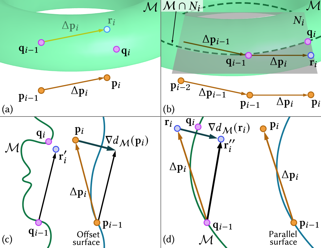
Figure 7. Anchored smooth-closest-point (a), and refinements: using a locally-fit plane (b), and anchor point constrained to an offset (c) or parallel surface (d). $\mathbf{q}_{i}$, is obtained by projecting $\mathbf{r}_{i}$ (a), $\mathbf{r}_{i}^{\prime}$ (c), or $\mathbf{r}_{i}^{\prime\prime}$ (d) onto $\mathcal{M}$ via smooth-closest-point; or closest-point to $\mathbf{r}_{i}$ in $\mathcal{M}\cap N_{i}$ (b).

Controller sampling rate in current VR systems is 50Hz or more, meaning that even during ballistic movements, the distance $\|\Delta\mathbf{p}_{i}\|$ for any stroke sample $i$ is of the order of a few millimetres. Consequently, the anchored stroke point $\mathbf{r}_{i}$ is typically much closer to $\mathcal{M}$, than the stroke point $\mathbf{p}_{i}$, making closest-point snap projection a compelling candidate for projecting $\mathbf{r}_{i}$. Such an anchored closest-point projection explicitly minimizes $\|\Delta\mathbf{p}_{i}-\Delta\mathbf{q}_{i}\|$, but precise minimization is less important than avoiding projection discontinuities and undesirably snapping, even for points close to the mesh. Our formulation of a smooth-closest-point projection $\pi_{SCP}$ in § 3.2 addresses these goals precisely. We define mimicry projection as

(4) $$\Pi_{mimicry}(\mathbf{p}_{i})=\begin{cases}\pi_{spray}(\mathbf{p}_{i})&\text{if }i=0,\\ \pi_{SCP}(\mathbf{r}_{i})&\text{otherwise.}\end{cases}$$

4.2. Refinements to Mimicry Projection

We further explore refinements to mimicry projection, that might improve curve projection in certain scenarios.

Planar curves are very common in design and visualization [McCrae et al., 2011]. We can locally encourage planarity in mimicry projection by constructing a plane $N_{i}$ with normal $\Delta\mathbf{p}_{i}\times\Delta\mathbf{p}_{i-1}$ (i.e. the local plane of the mid-air stroke) and passing through the anchor point $\mathbf{r}_{i}$ (Figure 7b). We then intersect $N_{i}$ with $\mathcal{M}$. $\mathbf{q}_{i}$ is defined as the closest-point to $\mathbf{r}_{i}$ on the intersection curve that contains $\mathbf{q}_{i-1}$. Note, we use $\pi_{spray}(\mathbf{p}_{i})$ for $i<2$, and we retain the most recently defined normal direction ($N_{i-1}$ or prior) when $N_{i}=\Delta\mathbf{p}_{i}\times\Delta\mathbf{p}_{i-1}$ is undefined. We find this method works well for near-planar curves, but the plane is sensitive to noise in the mid-air stroke (Figure 9f), and can feel sticky or less responsive for non-planar curves.

Offset and parallel surface drawing captures the observation that users tend to draw an intended curve as a corresponding stroke on an imaginary offset or parallel surface of the object $\mathcal{M}$. While we do not expect users to draw precisely on such surfaces, it is unlikely a user would intentionally draw orthogonal to them.

In scenarios when a user is sub-consciously drawing on an offset surface of $\mathcal{M}$ (an isosurface of its signed-distance function $d_{\mathcal{M}}(\cdot)$), we can remove the component of a user stroke segment along the gradient $\nabla d_{\mathcal{M}}$, when computing the anchor point (Figure 7c):

(5) $$\mathbf{r}_{i}^{\prime}=\mathbf{q}_{i-1}+\Delta\mathbf{p}_{i}-\Big{(}\Delta\mathbf{p}_{i}\cdot\nabla d_{\mathcal{M}}(\mathbf{p}_{i})\Big{)}\nabla d_{\mathcal{M}}(\mathbf{p}_{i})$$

We can similarly locally constrain user strokes to a parallel surface of $\mathcal{M}$ in Equation 6 as:

(6) $$\mathbf{r}_{i}^{\prime\prime}=\mathbf{q}_{i-1}+\Delta\mathbf{p}_{i}-\Big{(}\Delta\mathbf{p}_{i}\cdot\nabla d_{\mathcal{M}}(\mathbf{r}_{i})\Big{)}\nabla d_{\mathcal{M}}(\mathbf{r}_{i})\text{.}$$

Note that the difference from Eq. 5 is the position where $\nabla d_{\mathcal{M}}$ is computed, as shown in Figure 7d. A parallel surface better matched user expectation than an offset surface in our pilot testing, but both techniques produced poor results when user drawing deviated from these imaginary surfaces (Figure 9g–l).

4.3. Anchored Raycast Projection

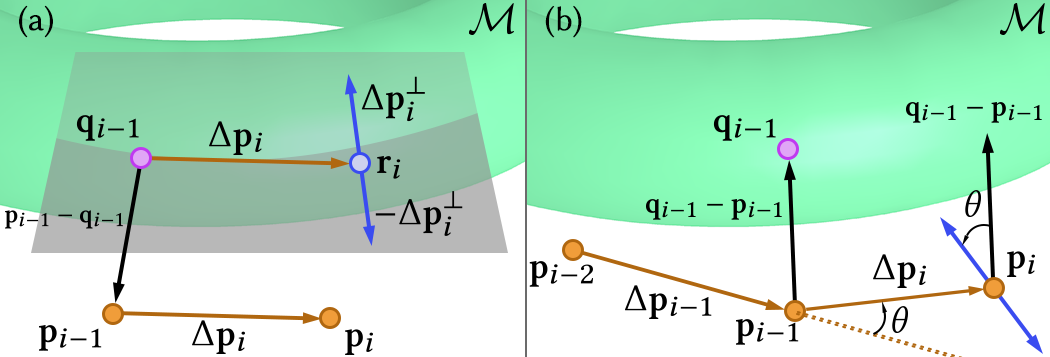
Figure 8. Anchored raycast techniques: ray direction defined orthogonal to $\Delta\mathbf{p}_{i}$ in a local plane (a); parallel transport of ray direction along the user stroke (b). The cast rays (forward/backward) are shown in blue.

For completeness, we also investigated raycast alternatives to projection of the anchored stroke point $\mathbf{r}_{i}$. We used similar priors of local planarity and offset or parallel surface transport as with mimicry refinement, to define ray directions. Figure 8 shows two such options.

In Figure 8a, we cast a ray in the local plane of motion, orthogonal to the user stroke, given by $\Delta\mathbf{p}_{i}$. We construct the local plane containing $\mathbf{r}_{i}$ spanned by $\Delta\mathbf{p}_{i}$ and $\mathbf{p}_{i-1}-\mathbf{q}_{i-1}$, and then define the direction orthogonal to $\Delta\mathbf{p}_{i}$ in this plane. Since $\mathbf{r}_{i}$ may be inside $\mathcal{M}$, we cast two rays bi-directionally $(\mathbf{r}_{i},\pm\Delta\mathbf{p}_{i}^{\bot})$, where

$$\Delta\mathbf{p}_{i}^{\bot}=\Delta\mathbf{p}_{i}\times\big{(}\Delta\mathbf{p}_{i}\times\left(\mathbf{p}_{i-1}-\mathbf{q}_{i-1}\right)\big{)}$$

If both rays successfully intersect $\mathcal{M}$, we choose $\mathbf{q}_{i}$ to be the point closer to $\mathbf{r}_{i}$. As with locally planar mimicry projection, this technique suffered from instability in the local plane.

Motivated by mimicry, we also explored parallel transport of the projection ray direction along the user stroke (Figure 8b). For $i>0$, we parallel transport the previous projection direction $\mathbf{q}_{i-1}-\mathbf{p}_{i-1}$ along the mid-air curve by rotating it with the rotation that aligns $\Delta\mathbf{p}_{i-1}$ with $\Delta\mathbf{p}_{i}$. Once again, bi-directional rays are cast from $\mathbf{r}_{i}$, and $\mathbf{q}_{i}$ is set to the closer intersection with $\mathcal{M}$.

In general, we found that all raycast projections, even when anchored, suffered from unpredictability over long strokes and discontinuities when there are no ray-object intersections (Figure 9n,o).

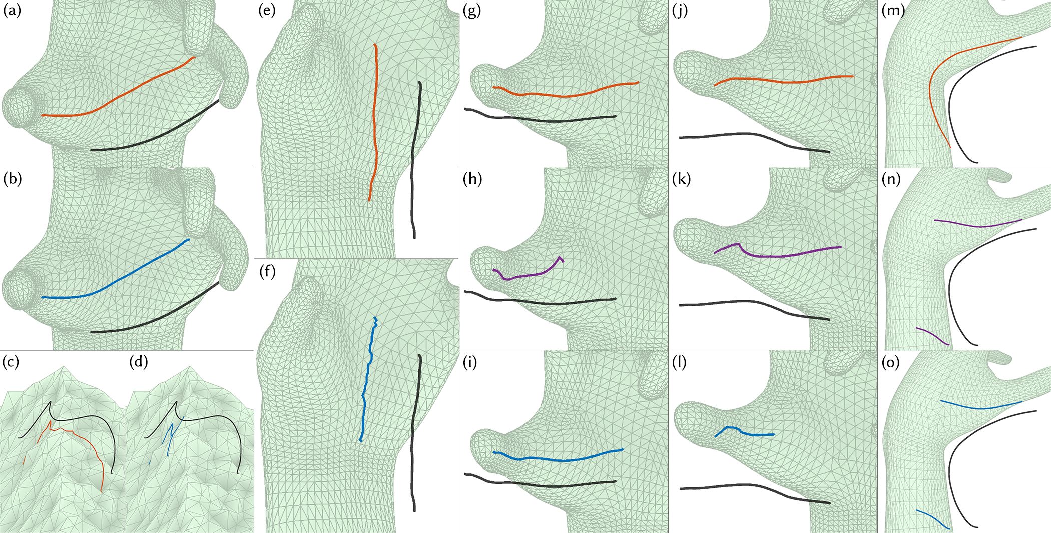
Figure 9. Mimicry vs. other anchored stroke projections: Mid-air strokes are shown in black and mimicry curves in red. Anchored closest-point (blue), is similar to mimicry on smooth, low-curvature meshes (a,b) but degrades with mesh detail/noise (c,d). Locally planar projection (blue) is susceptible local plane instability (e,f). Parallel (purple h,k) or offset (blue i,l) surface based projection fail in (h,l) when the user stroke deviates from said surface, while mimicry remains reasonable (g, j). Compared to mimicry (m), anchored raycasting based on a local plane (purple n), or ray transport (blue o) can be discontinuous.

4.4. Final Analysis and Implementation Details

In summary, extensive pilot testing of the anchored techniques revealed that they were generally better than context-free approaches, especially when users drew further away from the 3D object. Among anchored techniques, stroke mimicry captured as an anchored-smooth-closest-point projection proved to be theoretically elegant, and practically the most resilient to ambiguities of user intent and differences of drawing style among users. Anchored closest-point can be a reasonable proxy to anchored smooth-closest-point when pre-processing is undesirable. A pertinent application is real-time sculpting, where the object shape changes frequently.

Our techniques are implemented in C#, with interaction, rendering, and VR support provided by the Unity Engine. For the smooth closest-point operation, we modified Panozzo et al.’s [2013] reference implementation, which includes pre-processing code in MATLAB and C++, and real-time code in C++. The real-time projection implementation is exposed to our C# application via a compiled dynamic library. In their implementation, as well as ours, $d=8$; that is, we embed $\mathcal{M}$ in $\mathbb{R}^{8}$. Offset surfaces are computed using libigl [Jacobson et al., 2018], with $\mu=\|\mathtt{BBox}(\mathcal{M})\|/20$. We then improve surface quality using TetWild [Hu et al., 2018], before computing the tetrahedral mesh $\mathcal{T}_{\mathcal{M}}$ using TetGen [Si, 2015].

We support fast closest-point queries, using an AABB tree implemented in geometry3Sharp [Schmidt, 2017]. Signed-distance is also computed using the AABB tree and fast winding number [Barill et al., 2018], and gradient $\nabla d_{\mathcal{M}}$ computed using central finite differences.

To ease replication of our various techniques and aid future work, we have released our open-source implementation at github.com/ rarora7777/curve-on-surface-drawing-vr.

We now formally compare our most promising projection mimicry, to the best state-of-the-art context-free projection spraycan.

5. User Study

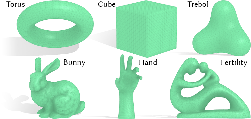
Figure 10. The six shapes utilized in the user study. The torus shape was used for tutorials, while the rest were used for the recorded experimental tasks.

We designed a user study to compare the performance of the spraycan and mimicry methods for a variety of curve-drawing tasks. We selected six shapes for the experiment (Figure 10), aiming to cover a diverse range of shape characteristics: sharp features (cube), large smooth regions (trebol, bunny), small details with ridges and valleys (bunny), thin features (hand), and topological holes (torus, fertility).

We then sampled ten distinct curves on the surface of each of the six objects. A canonical task in our study involved the participant attempting to re-create a given target curve from this set. We designed two types of drawing tasks shown in Figure 11:
Tracing curves, where a participant tried to trace over a visible target curve using a single smooth stroke.
Re-creating curves, where a participant attempted to re-create from memory, a visible target curve that was hidden as soon as the participant started to draw. An enumerated set of keypoints on the curve, however, remained as a visual reference, to aid the participant in re-creating the hidden curve with a single smooth stroke.

The rationale behind asking users to draw target curves is both to control the length, complexity, and nature of curves drawn by users, and to have an explicit representation of the user-intended curve. Curve tracing and re-creating are fundamentally different drawing tasks, each with important applications [Arora et al., 2017]. Our curve re-creation task is designed to capture free-form drawing, with minimal visual suggestion of intended target curve.

Target curves were sampled randomly from a distribution of long, smooth, curves on the mesh. For each sample curve, 4–9 keypoints were selected along endpoints and curvature extrema, the number depending on the curve’s length and complexity. Positioning keypoints at curvature extrema ensured that curve re-creating tasks amounted to smoothly joining the keypoints, rather than testing participants’ memory. Appendix B provides details about the sampling process.

5.1. Experiment Design

The main variable studied in the experiment was Projection method—spraycan vs. mimicry—realized as a within-subjects variable. The order of methods was counterbalanced between participants. For each method, participants were exposed to all the six objects. Object order was fixed as torus, cube, trebol, bunny, hand, and fertility, based on our personal judgment of drawing difficulty. The torus was used as a tutorial, where participants had access to additional

instructions visible in the scene and their strokes were not utilized for analysis. For each object, the order of the 10 target strokes was randomized. The first five were used for the tracing curves task, while the remaining five were used for re-creating curves.

The target curve for the first tracing task was repeated after the five unique curves, to gauge user consistency and learning effects. A similar repetition was used for curve re-creation. Participants thus performed 12 curve drawing tasks per object, leading to a total of $12\times 5$ (objects) $\times\ 2$ (projections) $=120$ strokes per participant.

Owing to the COVID-19 physical distancing guidelines, the study was conducted on participants’ personal VR equipment at their homes. A 15-minute instruction video introduced the study tasks and the two projection methods. Participants then filled out a consent form and a questionnaire to collect demographic information. This was followed by them testing the first projection method and filling out a questionnaire to express their subjective opinions of the method. They then tested the second method, followed by a similar questionnaire, and questions involving subjective comparisons between the two methods. Participants were required to take a break after testing the first method, and were also encouraged to take breaks after drawing on the first three shapes for each method. The study took approximately an hour, including the questionnaires.

5.2. Participants

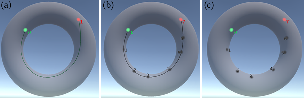
Figure 11. Study tasks—curve tracing: target curve is visible when drawing (a), and curve re-creation: target curve (b) is hidden when drawing (c).

Twenty participants (5 female, 15 male) aged 21–47 from five countries participated in the study. All but one were right-handed. Participants were not selected for artistic ability or prior VR experience, and exhibited a diverse range of self-reported artistic abilities (min. 1, max. 5, median 3 on a 1–5 scale) as well as varying degrees of VR experience, ranging from below 1 year to over 5 years. 13 participants had a technical computer graphics or HCI background, while ten had experience with creative tools in VR, with one reporting professional usage. Participants were paid $\approx 22$ USD as a gift card.

5.3. Apparatus

As the study was conducted on personal VR setups, a variety of commercial VR devices were utilized—Oculus Rift, Rift S, and Quest using Link cable, HTC Vive and Vive Pro, Valve Index, and Samsung Odyssey using Windows Mixed Reality. All but one participant used a standing setup allowing them to freely move around.

5.4. Procedure

Before each trial, participants could use the “grab” button on their controller (in the dominant hand) to grab the mesh to position and orient it as desired. The trial started as soon as the participant started to draw by pressing the “main trigger” on their dominant hand controller. This action disabled the grabbing interaction—participants could not draw and move the object simultaneously. As noted earlier, for curve re-creation tasks, this had the additional effect of hiding the target curve, but leaving keypoints visible.

6. Study Results and Discussion

We recorded the head position $\mathbf{h}$ and orientation $\mathsf{h}$, controller position $\mathbf{c}$ and orientation $\mathsf{c}$, projected point $\mathbf{q}$, and timestamp $t$, for each mid-air stroke point $\mathbf{p}=\mathbf{c}$. We refer to a target curve as $\mathcal{X}$, a mid-air stroke as $\mathcal{P}$, and a projected curve as $\mathcal{Q}$.

6.1. Data Processing and Filtering

We formulated three criteria to filter out meaningless user strokes.

Short Curves

We ignore projected curves $\mathcal{Q}$ that are too short as compared to the length of the target curves $\mathcal{X}$ (conservatively curves less than half as long as the target curve). While it is possible that the user stopped drawing mid-way out of frustration, we found it was more likely that they prematurely released the controller trigger by accident. Both curve lengths are computed in $\mathbb{R}^{3}$ for efficiency.

Stroke Noise

We ignore strokes for which the mid-air stroke is too noisy. Specifically, mid-air strokes with distant consecutive points ($\exists\ i\ \text{s.t.}\ \|\mathbf{p}_{i}-\mathbf{p}_{i-1}\|>5\text{cm}$) are rejected.

Inverted Curves

While we labelled keypoints with numbers and marked start and end points in green and red (Figure 11), some users occasionally drew the target curve in reverse. The motion to draw a curve in reverse is not symmetric, and such curves are thus rejected. We detect inverted strokes by looking at the indices $i_{0},i_{1},\ldots,i_{l}$ of the points in $\mathcal{Q}$ which are closest to the keypoints $\mathbf{x}_{k_{0}},\mathbf{x}_{k_{1}},\ldots,\mathbf{x}_{k_{l}}$ of $\mathcal{X}$. Ideally, the sequence $i_{0},\ldots,i_{l}$ should have no inversions, i.e., $\forall\ 0\leq j<k\leq l,\ i_{j}\leq i_{k}$; and maximum $l(l+1)/2$ inversions, if $\mathcal{Q}$ is aligned in reverse with $\mathcal{X}$. We consider curves with more than $l(l+1)/4$ (half the maximum) inversions to be inadvertently inverted and reject them. Distances are computed in $\mathbb{R}^{3}$ for efficiency.

Despite conducting our experiment remotely without supervision, we found that 95.8% of the strokes satisfied our criteria and could be utilized for analysis. Out of the 102 strokes deemed unfit for analysis, 17 were too short, 66 were inverted, and 38 exhibited excessive tracking noise. It is possible that some of the short or inverted curves were caused due to curve control issues, there is no robust automatic method for distinguishing between inadvertent errors and genuine challenges faced by the users. Given the small number of such strokes and the potential bias in manual classification, we chose to exclude these strokes from the analysis. For comparisons between $\pi_{spray}$ and $\pi_{mimicry}$, we reject stroke pairs where either stroke did not satisfy the quality criteria. Out of 1200 pairs (2400 total strokes), 1103 (91.9%) satisfied the quality criteria and were used for analysis, including 564 pairs for the curve re-creation task and 539 for the tracing task.

Table 2. Quantitative results (mean $\pm$ std. dev.) of the comparisons between mimicry and spraycan projection. All measures are analyzed using Wilcoxon signed-rank tests, lower values are better, and significantly better values ($p<.05$) are shown in boldface. Accuracy, aesthetic, and physical effort measures are shown with green, red, and blue backgrounds, respectively.

Tracing Curves
Measure	Spraycan	Mimicry	$p$-value	$z$-stat
$D_{ep}$	2.31 $\pm$ 2.64 mm	1.13 $\pm$ 1.11 mm	¡.001	8.36
$D_{sym}$	0.64 $\pm$ 0.66 mm	0.56 $\pm$ 0.44 mm	¿.05	-0.09
$K_{E}$	280 $\pm$ 262 rad/m	174 $\pm$ 162 rad/m	¡.001	15.59
$K_{g}$	249 $\pm$ 245 rad/m	152 $\pm$ 157 rad/m	¡.001	15.42
$F_{g}$	394 $\pm$ 413 rad/m	248 $\pm$ 285 rad/m	¡.001	14.82
$T_{h}$	0.81 $\pm$ 0.70	0.58 $\pm$ 0.40	¡.001	7.93
$R_{h}$	1.63 $\pm$ 2.18 rad/m	1.18 $\pm$ 1.63 rad/m	¡.001	4.82
$T_{c}$	1.05 $\pm$ 0.36	1.10 $\pm$ 0.29	¡.001	-3.36
$R_{c}$	5.12 $\pm$ 5.88 rad/m	3.79 $\pm$ 4.84 rad/m	¡.001	5.51
$\tau$	4.69 $\pm$ 1.85 s	5.29 $\pm$ 2.17 s	¡.001	-7.32
Re-creating Curves
Measure	Spraycan	Mimicry	$p$-value	$z$-stat
$D_{ep}$	2.34 $\pm$ 2.49 mm	2.24 $\pm$ 23.32 mm	¡.001	8.63
$D_{sym}$	0.75 $\pm$ 0.65 mm	1.12 $\pm$ 11.51 mm	¿.05	0.55
$K_{E}$	254 $\pm$ 236 rad/m	155 $\pm$ 127 rad/m	¡.001	14.70
$K_{g}$	223 $\pm$ 219 rad/m	132 $\pm$ 123 rad/m	¡.001	14.95
$F_{g}$	348 $\pm$ 371 rad/m	215 $\pm$ 227 rad/m	¡.001	14.11
$T_{h}$	0.72 $\pm$ 0.54	0.54 $\pm$ 0.35	¡.001	6.78
$R_{h}$	1.50 $\pm$ 2.19 rad/m	1.32 $\pm$ 1.99 rad/m	.002	3.07
$T_{c}$	1.05 $\pm$ 0.37	1.11 $\pm$ 0.23	¡.001	-5.94
$R_{c}$	5.23 $\pm$ 6.36 rad/m	3.63 $\pm$ 5.13 rad/m	¡.001	4.00
$\tau$	4.33 $\pm$ 1.57 s	4.92 $\pm$ 1.89 s	¡.001	-7.12

6.2. Quantitative Analysis

We define 10 different statistical measures (Table 2) to compare $\pi_{spray}$ and $\pi_{mimicry}$ curves in terms of their accuracy, aesthetic, and effort in curve creation. We consistently use the non-parametric Wilcoxon signed rank test for all quantitative measures instead of a parametric test such as the paired $t$-test, since the recorded data for none of our measures was normally distributed (normality hypothesis rejected via the Kolmogorov-Smirnov test, $p<.005$). In addition, we analyze users’ tendency to mimic the target strokes and consistency between repeated strokes in Appendix C.

6.2.1. Curve Accuracy

Accuracy is computed using two measures of distance between points on the projected curve $\mathcal{Q}$ and target curve $\mathcal{X}$. Both curves are densely re-sampled using $m=101$ sample points equi-spaced by arc-length.

Given $\mathcal{Q}={\mathbf{q}_{0},\ldots,\mathbf{q}_{m-1}}$ and $\mathcal{X}={\mathbf{x}_{0},\ldots,\mathbf{x}_{m-1}}$, we compute the average equi-parameter distance $D_{ep}$ as

(7) $$D_{ep}(\mathcal{Q})=\frac{1}{m}\sum_{i=0}^{m-1}d_{E}\left(\mathbf{q}_{i},\mathbf{x}_{i}\right)\text{,}$$

where $d_{E}$ computes the Euclidean distance between two points in $\mathbb{R}^{3}$. We also compute the average symmetric distance $D_{sym}$ as

$$D_{sym}(\mathcal{Q})=\frac{1}{2m}\sum_{i=0}^{m-1}\left(\min_{\mathbf{x}\in X}d_{E}\left(\mathbf{q}_{i},\mathbf{x}\right)\right)+\frac{1}{2m}\sum_{i=0}^{m-1}\left(\min_{\mathbf{q}\in Q}d_{E}\left(\mathbf{q},\mathbf{x}_{i}\right)\right)$$

In other words, $D_{ep}$ computes the distance between corresponding points on the two curves and $D_{sym}$ computes the average minimum distance from each point on one curve to the other curve.

For both tracing and re-creation tasks, $D_{ep}$ indicated that mimicry produced significantly better results than spraycan (see Table 2, Figure 1c, 12). The $D_{sym}$ difference was not statistically significant, evidenced by users correcting their strokes to stay close to the intended target curve (at the expense of curve aesthetic).

6.2.2. Curve Aesthetic

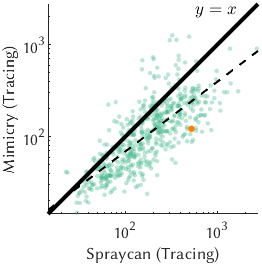
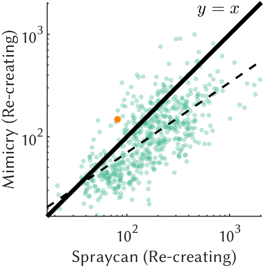
(a) Normalized geodesic curvature $K_{g}$.

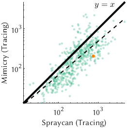
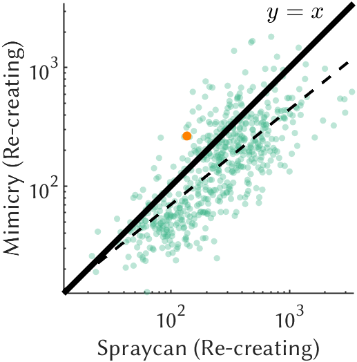
(b) Normalized fairness deficiency $F_{g}$.

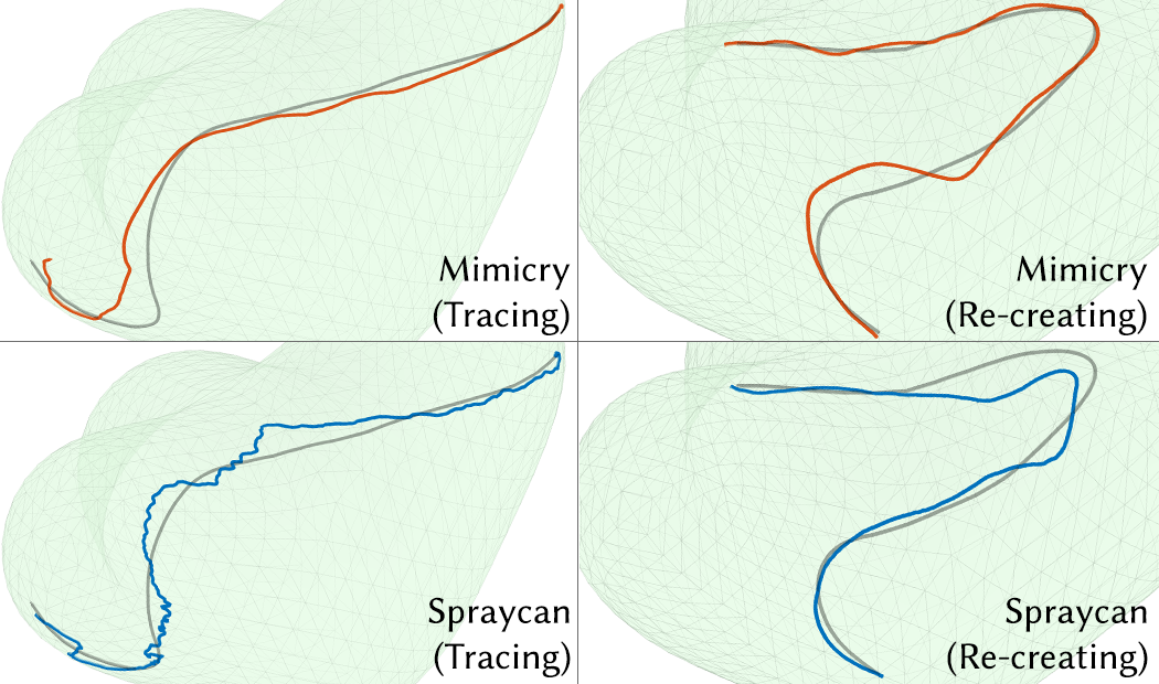
(c) Example strokes, orange points in (a, b) above.

Figure 12. Curvature measures (a,b) indicate that mimicry produces significantly smoother and fairer curves than spraycan for both tracing (left) and re-creating tasks (right). Pairwise comparison plots between mimicry (y-axis) and spraycan (x-axis), favour mimicry for the vast majority of points (points below the $y=x$ line). A linear regression fit (on the log plots) is shown as a dashed line. Example curve pairs (orange points) for curve tracing and re-creating are also shown with the target curve $\mathcal{X}$ shown in gray (c).

For most design applications, jagged projected curves, even if geometrically quite accurate, are aesthetically undesirable [McCrae and Singh, 2008]. Curvature-based measures are typically used to measure fairness of curves. We report three such measures of curve aesthetic for the projected curve $\mathcal{Q}=\mathbf{q}_{0},\ldots,\mathbf{q}_{n-1}$. We first refine $\mathcal{Q}$ by computing the exact geodesic on $\mathcal{M}$ between consecutive points of $\mathcal{Q}$  [Surazhsky et al., 2005], to create $\widehat{\mathcal{Q}}$ with points $\widehat{\mathbf{q}}_{0},\ldots,\widehat{\mathbf{q}}_{k-1}$, $k\geq n$. We choose to normalize our curvature measures using $L_{\mathcal{X}}$, the length of the corresponding target stroke $\mathcal{X}$. The normalized Euclidean curvature for $\mathcal{Q}$ is defined as

(8) $$K_{E}(\mathcal{Q})=\frac{1}{L_{\mathcal{X}}}\sum_{i=1}^{k-2}\theta_{i}$$

where $\theta_{i}$ is the angle between the two segments of $\widehat{\mathcal{Q}}$ incident on $\widehat{\mathbf{q}}_{i}$. Thus, $K_{E}$ is the total discrete curvature of $\widehat{\mathcal{Q}}$, normalized by the target curve length.

Since $\widehat{\mathcal{Q}}$ is embedded in $\mathcal{M}$, we can also compute discrete geodesic curvature, computed as the deviation from the straightest geodesic on a surface. Using a signed $\theta^{g}_{i}$ defined at each point $\widehat{\mathbf{q}}_{i}$ [Polthier and Schmies, 2006], we compute normalized geodesic curvature as

(9) $$K_{g}(\mathcal{Q})=\frac{1}{L_{\mathcal{X}}}\sum_{i=1}^{k-2}|\theta_{i}^{g}|\text{.}$$

Finally, we define fairness [Arora et al., 2017; McCrae and Singh, 2008] as a first-order variation in geodesic curvature, thus defining the normalized fairness deficiency as

(10) $$F_{g}(\mathcal{Q})=\frac{1}{L_{\mathcal{X}}}\sum_{i=2}^{k-2}|\theta_{i}^{g}-\theta_{i-1}^{g}|\text{,}$$

For all three measures, a lower value indicates a smoother, pleasing, curve. Wilcoxon signed-rank tests on all three measures indicated that mimicry produced significantly smoother and better curves than spraycan (Table 2).

6.2.3. Physical Effort

The amount of head (HMD) and hand (controller) movement, and stroke execution time $\tau$ provide quantitative proxies for physical effort.

For head and hand translation, we first filter the position data with a Gaussian-weighted moving average filter with $\sigma=20\text{ms}$. We then define normalized head/controller translation $T_{h}$ and $T_{c}$ as the length of the poly-line defined by the filtered head/controller positions normalized by the length of the target curve $L_{\mathcal{X}}$.

An important ergonomic measure is the amount of head/hand rotation required to draw the mid-air stroke. We first de-noise or filter the forward and up vectors of the head/controller frame, using the same filter as for positional data. We then re-orthogonalize the frames and compute the length of the curve defined by the filtered orientations in $\mathrm{SO(3)}$, using the angle between consecutive orientation data-points. We define normalized head/controller rotation $R_{h}$ and $R_{c}$ as its orientation curve length, normalized by $L_{\mathcal{X}}$.

Table 2 summarizes the physical effort measures. We observe lower controller translation (effect size $\approx 5\%$) and execution time (effect size $\approx 12\%$) in favour of spraycan; lower head translation and orientation (effect sizes $\approx 36\%,26\%$) in favour of mimicry. Noteworthy is the significantly reduced controller rotation using mimicry, with spraycan unsurprisingly requiring $35\%$ (tracing) and 44% (re-creating) more hand rotation from the user.

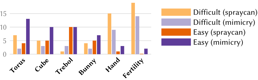
Figure 13. Perceived difficulty of drawing for the six 3D shapes in the study.

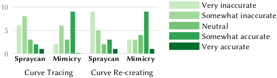
(a) Perceived accuracy.

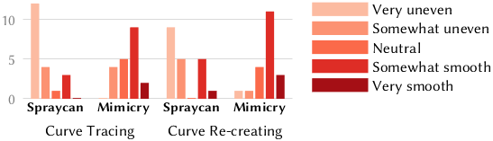
(b) Perceived smoothness.

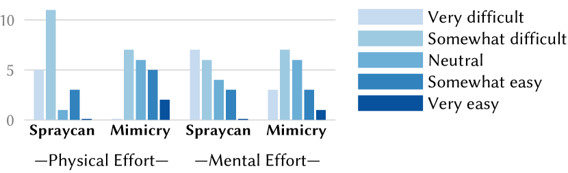
(c) Physical and mental effort ratings.

Figure 14. Participants perceived mimicry to be better than spraycan in terms of accuracy (a), curve aesthetic (b) and user effort (c).

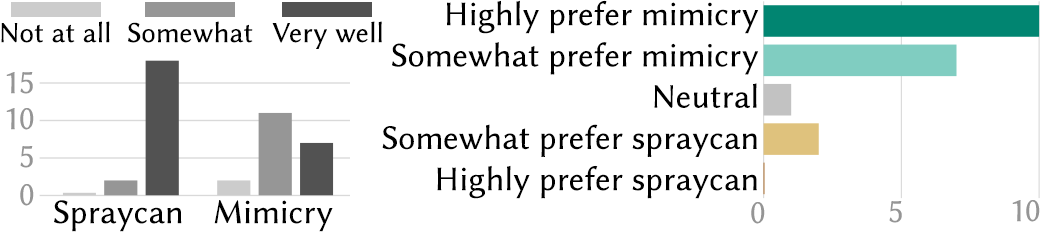
Figure 15. Participants stated understanding spraycan projection better (left); 17/20 users stated an overall preference for mimicry over spraycan (right).

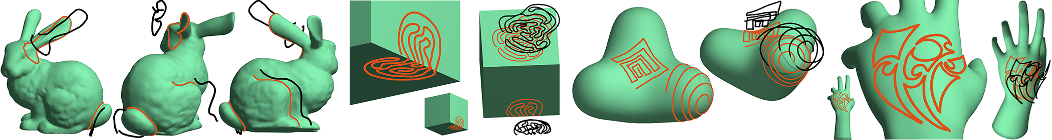
Figure 16. Gallery of free-form curves in red, drawn by the paper authors using mimicry. (Left to right) tracing geometric features on the bunny, maze-like curves on the cube, maze with sharp corners and a spiral on the trebol, and artistic tattoo motifs on the hand. Some mid-air strokes (black) hidden for clarity.

6.3. Qualitative Analysis

The mid- and post-study questionnaires elicited qualitative responses from participants on their perceived difficulty of drawing, curve accuracy and smoothness, mental and physical effort, understanding of the projection methods, and overall method of preference.

Participants were asked to specify the objects which they found especially easy or difficult to draw on, when using either of the two projection methods. In general, the shapes shown earlier were judged to be easier to work with (Figure 13), validating our ordering of shapes in the experiment based on expected drawing difficulty. Importantly, this observation also suggests a lack of any learning effects caused by the fixed object ordering.

Accuracy, smoothness, physical/mental effort responses were collected via 5-point Likert scales. We consistently order the choices from 1 (worst) to 5 (best) in terms of user experience, and report median ($M$) scores here. Mimicry was perceived to be a more accurate projection (tracing, re-creating $M=3,3.5$) compared to spraycan ($M=2,2$), with 9 participants perceiving their traced curves to be either very accurate or somewhat accurate with mimicry, compared to 2 for spraycan (Figure 14a). Perception of stroke smoothness was also consistent with quantitative results, with mimicry (tracing, re-creating $M=4,4$) clearly outperforming spraycan (tracing, re-creating $M=1,2$) (Figure 14b). Lastly, with no need for controller rotation, mimicry ($M=3$) was perceived as less physically demanding than spraycan ($M=2$), as expected (Figure 14c).

The response to understanding and mental effort was more complex. Spraycan, with its physical analogy and mathematically precise definition was clearly understood by all 20 participants (17 very well, 3 somewhat) (Figure 15a). Mimicry, conveyed as “drawing a mid-air stroke on or near the object as similar in shape as possible to the intended projection”, was less clear to users (7 very well, 11 somewhat, 3 not at all). Despite not understanding the method consciously, the 3 participants were able to create curves that were both accurate and smooth. Further, users perceived mimicry ($M=2.5$) as less cognitively taxing than spraycan ($M=2$) (Figure 14c). We believe this may be because users were less prone to consciously controlling their stroke direction and rather focused on drawing. The tendency to mimic may have thus manifested sub-consciously, as we had observed in pilot testing.

The most important qualitative question was user preference (Figure 15b). $85\%$ of the 20 participants preferred mimicry (10 highly preferred, 7 somewhat preferred). The remaining users were neutral (1/20) or somewhat preferred spraycan (2/20).

6.4. Participant Feedback

We also asked participants to elaborate on their stated preferences and ratings. Participants (P4,8,16,17) noted discontinuous “jumps” caused by spraycan, and felt the continuity guarantee of mimicry: “seemed to deal with the types of jitter and inaccuracy VR setups are prone to better” (P6) ; “could stabilize my drawing” (P9) . P9,15 felt that mimicry projection was smoothing their strokes (no smoothing was employed): we believe this may be the effect of noise and inadvertent controller rotation, which mimicry ignores, but can cause large variations with spraycan, perceived as curve smoothing.

Some participants (P4,17) felt that rotating the hand smoothly while drawing was difficult, while others missed the spraycan ability to simply use hand rotation to sweep out long projected curves from a distance (P2,7). Participants commented on physical effort: “Mimicry method seemed to required [sic] much less head movement, hand rotation and mental planning” (P4) .

Participants appreciated the anchored control of mimicry in high-curvature regions (P1,2,4,8) also noting that with spraycan, “the curvature of the surface could completely mess up my stroke” (P1) . Some participants did feel that spraycan could be preferable when drawing on near-flat regions of the mesh (P3,14,19,20).

Finally, participants who preferred spraycan felt that mimicry required more thinking: “with mimicry, there was extra mental effort needed to predict where the line would go on each movement” (P3) , or because mimicry felt “unintuitive” (P7) due to their prior experience using a spraycan technique. Some who preferred mimicry found it difficult to use initially, but felt it got easier over the course of the experiment (P4,17).

7. Applications

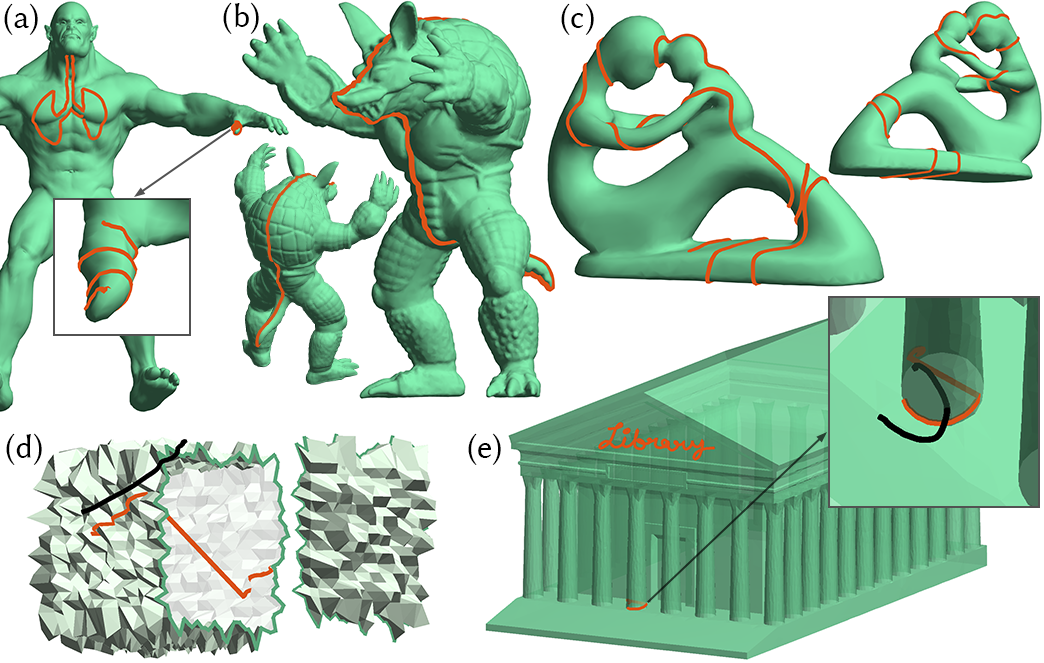
Figure 17. Mimicry can be used to draw long, complicated curves on complex high-resolution meshes. We show strokes on high-resolution meshes (a, b, e), a long stroke bisecting a model (b), and a single stroke winding around a topologically non-trivial object multiple times (c). However, excessive noise in the input mesh can break the underlying $\pi_{ACP}$ assumptions, resulting in catastrophic failure (d). Mesh has been cut open for visualization. Large meshes with many sharp features and topological complexity can also show smaller local failures in the form of unexpected jumps when drawing close to the sharp features (e, inset).

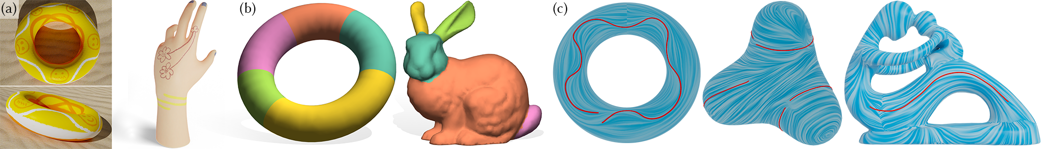
Figure 18. Applications of mimicry projection. Texture painting (a), interactive segmentation by drawing curves onto meshes (b), and providing constraints (red curves) to guide the vector field generation of Fisher et al. [2007] (c).

Complex 3D curves on arbitrary surfaces can be drawn in VR with a single stroke, using mimicry (Figure 16). Drawing such curves on 3D virtual objects is fundamental to many applications, including direct painting of textures  [Schmidt et al., 2006]; tangent vector field design [Fisher et al., 2007]; texture synthesis [Turk, 2001; Lefebvre and Hoppe, 2006]; interactive selection, annotation, and object segmentation [Chen et al., 2009]; and seams for shape parametrization [Lévy et al., 2002; Rabinovich et al., 2017; Sawhney and Crane, 2017], registration [Gehre et al., 2018], and quad meshing [Tong et al., 2006]. We showcase the utility and quality of mimicry curves within example applications (also see supplemental video).

We also stress-test our technique by drawing curves on complex models (Figure 17a,b,e) and drawing a single long curve looping around the fertility model multiple times (Figure 17c). Finally, we show a failure case discussed in § 3.2—the mimicry projection fails catastrophically due to problems in the underlying $\pi_{ACP}$ projection when the mesh is perturbed with excessive random noise (Figure 17d). Smaller local jumps can also occur when the model is both highly detailed and contains many sharp features (see inset in Figure 17e).

Texture Painting

Figures 1e, 18a show examples of textures painted in VR using mimicry. The long, smooth, wraparound curves on the torus, are especially hard to draw with 2D interfaces. Our implementation uses Discrete Exponential Maps (DEM) [Schmidt et al., 2006] to compute a dynamic local parametrization around each projected point $\mathbf{q}_{i}$, to create brush strokes or geometric stamps on the object.

Mesh Segmentation

Figures 1e, 18b show interactive segmentation using mimicry. In our implementation, users draw an almost-closed curve $\mathcal{Q}=\{\mathbf{q}_{0},\ldots,\mathbf{q}_{n-1}\}$ on the object using mimicry. We snap points $\mathbf{q}_{i}$ to their nearest mesh vertex, and use Dijkstra’s shortest path to connect consecutive vertices, and to close the cycle. While easy in VR via mimicry, drawing similar strokes in 2D for selection/segmentation would require multiple view changes.

Vector Field Design

Vector fields on meshes are commonly used for texture synthesis [Turk, 2001], guiding fluid simulations [Stam, 2003], and non-photorealistic rendering [Hertzmann and Zorin, 2000]. We use mimicry curves as soft constraints to guide the vector field generation of Fisher et al. [2007]. Figure 18c shows example vector fields, visualized using Line Integral Convolutions [Cabral and Leedom, 1993] in the texture domain.

8. Conclusion

We have presented a detailed investigation of the problem of real-time inked drawing on 3D virtual objects in immersive environments. We show the importance of stroke context when projecting mid-air 3D strokes, and explore the design space of anchored projections. A 20-participant study showed mimicry to be preferred over the established spraycan projection for projecting 3D strokes onto objects in VR. Both mimicry projection and performing VR studies in the wild do have some limitations. Further, while user stroke processing for 2D interfaces is a mature field of research, mid-air stroke processing for AR/VR is relatively nascent, with many directions for future work. Our study contributes a high-quality VR data corpus comprising $\approx 2400$ user strokes, projected curves, intended target curves, and corresponding system states, useful for future data-driven techniques for mid-air stroke processing.

“In the wild” VR Study Limitations

Ongoing pandemic restrictions presented both a challenge and an opportunity to remotely conduct a more natural study in the wild, with a variety of consumer VR hardware and setups. The enthusiasm of the VR community allowed us to readily recruit 20 diligent users, albeit with a bias towards young, adult males. While the variation in VR headsets seemed to be of little consequence, differences in controller grip and weight can certainly impact mid-air drawing posture and stroke behavior. Controller size is also significant: a larger Vive controller, for example, has a higher chance of occluding target objects and projected curves, as compared to a smaller Oculus Touch controller. We could have mitigated the impact of controller size by rendering a standard drawing tool, but we preferred to render the familiar, default controller that matched the physical device in participants’ hands. Further, no participant explicitly mentioned the controller getting in the way of their ability to draw.

Mimicry Limitations

Our lack of a concise mathematical definition of observed stroke mimicry, makes it harder to precisely communicate it to users. While a precise mathematical formulation may exist, conveying it to non-technical users can still be a challenging task. Mimicry ignores controller orientation, producing smoother strokes with less effort, but can give participants a reduced sense of sketch control (P2,3,6). We hypothesize that the reduced sense of control is in part due to the tendency for anchored smooth-closest-point to shorten the user stroke upon projection, sometimes creating a feeling of lag. Spraycan like techniques, in contrast, have a sense of amplified immediacy, and the explicit ability to make lagging curves catch-up by rotating a controller in place.

Future work

Our goal was to develop a general real-time inked projection with minimal stroke context via anchoring. Optimizing the method to account for the entire partially projected stroke may improve the projection quality. Relaxing the restriction of real-time inking would allow techniques such as spline fitting and global optimization that can account for the entire user stroke and geometric features of the target object. Local parametrizations such as DEM (§ 7) can be used to incrementally grow or shrink the projected curve, so it does not lag the user stroke. Hybrid projections leveraging both proximity and raycasting are also subject to future work.

On the interactive side, we experimented with feedback to encourage users to draw closer to a 3D object. For example, we tried varying the appearance of the line connecting the controller to the projected point based on line length; or providing aural/haptic feedback if the controller got further than a certain distance from the object. While these techniques can help users in specific drawing or tracing tasks, we found them to be distracting and harmful to stroke quality for general stroke projection. Bimanual interaction, such as rotating the shape with one hand while drawing on it with the other (suggested by P3,19), can also be explored. To generalize our work to AR, the impact of rendering quality and perception of virtual models also needs to be studied in the future. Drawing on physical objects in AR is another related research direction.

Application-dependent optimizations to encourage closed strokes, snapping to geometric features, or alignment with existing user-drawn curves, can also be explored in the future. Further, our user study only focused on smooth curves. While we show author-drawn example of curves with sharp features (Figure 16), formally testing the mimicry technique for drawing such curves and potentially optimizing the projection to deal with sharp features is an important future direction. But perhaps the most exciting area of future work is data-driven techniques for inferring the intended projection, perhaps customized to the drawing style of individual users. Our study code and data has been made publicly available at github.com/rarora7777/curve-on-surface-drawing-vr to aid in such endeavours.

Appendix A Context-Free Pilot Observations

In this appendix, we provide additional informal observations from our pilot tests with context-free techniques (Section 3.1), as well as additional details on the limitations of such techniques.

A.1. Qualitative observations

• Head-centric and occlude projections become unpredictable if the user is inadvertently changing their viewpoint while drawing. These projections are also only effective when drawing frontally on an object, like with a 2D interface. Neither as a result exploits the potential gains of mid-air drawing in AR/VR.

• Spraycan projection was clearly the most effective context-free technique. We noted however, that consciously reorienting the controller while drawing on or around complex objects was both cognitively and physically tiring.

• Snap projection was quite sensitive to changes in the distance of the stroke from the object surface, and in general produced the most undulating projections due to closest-point singularities.

• All projections converge to the mid-air user stroke when it precisely conforms to the surface of the 3D object. But as the distance between the object and points on the mid-air stroke increases, their behavior diverges quickly.

• While users did draw in the vicinity and mostly above the object surface, they rarely drew precisely on the object. The average distance of stroke points from the target object was observed to be 4.8 cm in a subsequent user study (§ 5).

A.2. Details on the Limitations of Context-Free Methods

The inability of context-free approaches to capture a notion of stroke mimicry—due to a lack of curve history or context—materializes as problems in different forms.

A.2.1. Projection Discontinuities

Proximal projection (including smooth-closest-point) can be highly discontinuous with increasing distance from the 3D object, particularly in concave regions (Figure 5a). Mid-air drawing along valleys without staying in precise contact with virtual object is thus extremely difficult. Raycast projections can similarly suffer large discontinuous jumps across occluded regions (in the ray direction) of the object (Figure 5d).

While this problem theoretically exists in 2D interfaces as well, it is less observed in practice for two reasons: 2D drawing on a constraining physical surface is significantly more precise than mid-air drawing in AR/VR [Arora et al., 2017]; and artists minimize such discontinuities by carefully choosing appropriate views (raycast directions) before drawing each curve. Automatic direction control of view or controller, while effective in 2D [Ortega and Vincent, 2014]), is detrimental to a sense of agency and presence in AR/VR.

A.2.2. Undesirable Snapping

Proximity-based methods also tend to get stuck on sharp (or high curvature) convex features of the object (Figure 5b). While this can be useful to trace along a ridge feature, it is particularly problematic for general curve-on-surface drawing.

A.2.3. Projection depth disparity

The relative orientation between the 3D object surface and raycast direction can cause large depth disparities between parts of user strokes and curves projected by raycasting (Figure 5c). Such irregular bunching or spreading of points on the projected curve also goes against our observation of stroke mimicry. Users can arguably reduce this disparity by continually orienting the view/controller to keep the projection ray well aligned with object surface normal. Such re-orientation however can be tiring, ergonomically awkward, and deviates from 2D experience, where pen/brush tilt only impacts curve aesthetic, and not shape.

Appendix B Sampling Target Curves for the User Study

We wanted to design target curves that could be executed using a single smooth motion. Since users typically draw sharp corners using multiple strokes [Bae et al., 2008], we constrain our target curves to be smooth, created using cardinal cubic B-splines on the meshes, computed using Panozzo et al. [2013]. We also control the length and curvature complexity of the curves, as pilot testing showed that very simple and short curves can be reasonably executed by almost any projection technique. Curve length and complexity is modeled by placing spline control points at mesh vertices, and specifying the desired geodesic distance and Gauß map distance between consecutive control points on the curve.

We represent a target curve using four parameters $\langle n,i_{0},k_{G},k_{N}\rangle$, where $n$ is the number of spline control points, $i_{0}$ the vertex index of the first control point, and $k_{G},k_{N}$ constants that control the geodesic and normal map distance between consecutive control points. We define the desired geodesic distance between consecutive control points as, $D_{G}=k_{G}\times\|\mathtt{BBox}(\mathcal{M})\|$, where $\|\mathtt{BBox}(\mathcal{M})\|$ is the length of the bounding box diagonal of $\mathcal{M}$. The desired Gauß map distance (angle between the unit vertex normals) between consecutive control points is simply $k_{N}$.

A target curve $\mathbf{C}_{0},\ldots,\mathbf{C}_{n-1}$ starting at vertex $\mathbf{v}_{i_{0}}$ of the mesh is generated incrementally for $i>0$ as:

(11) $$\mathbf{C}_{i}=\operatorname*{arg\,min}_{\mathbf{v}\in V^{\prime}}\ \big{(}d_{G}(\mathbf{C}_{i-1},\mathbf{v})-D_{G}\big{)}^{2}+\big{(}d_{N}(\mathbf{C}_{i-1},\mathbf{v})-k_{N}\big{)}^{2},$$

where $d_{G}$ and $d_{N}$ compute the geodesic and normal distance between two points on $\mathcal{M}$, and $V^{\prime}\subset V$ contains only those vertices of $\mathcal{M}$ whose geodesic distance from $\mathbf{C}_{0},\ldots,\mathbf{C}_{i-1}$ is at least $D_{G}/2$. The restricted subset of vertices conveniently helps prevent (but doesn’t fully avoid) self-intersecting or nearly self-intersecting curves. Curves with complex self-intersections are less important practically, and can be particularly confusing for the curve re-creation task. All our target curve samples were generated using $k_{G}\in[0.05,0.25]$, $k_{N}\in[\pi/6,5\pi/12]$, $n=6$, and a randomly chosen $i_{0}$. The curves were manually inspected for self-intersections, and infringing curves rejected.

We then defined keypoints on the target curves as follows: curve endpoints were chosen as keypoints; followed by greedily picking extrema of geodesic curvature, while ensuring that the arclength distance between any two consecutive keypoints was at least 3cm; and concluding the procedure when the maximum arclength distance between any consecutive keypoints was below 15cm. Our target curves had between 4–9 keypoints (including endpoints).

Appendix C Additional Quantitative Analyses

C.1. Quantifying Users’ Tendency to Mimic

The study also provided an opportunity to test if the users actually tended to mimic their intended curve $\mathcal{X}$ in the mid-air stroke $\mathcal{P}$. To quantify the “mimcriness” of a stroke, we subsample $\mathcal{P}$ and $\mathcal{X}$ into $m$ points as in § 6.2.1, use the correspondence as in Eq. 7 and look at the variation in the distance (distance between the closest pair of corresponding points subtracted from that of the farthest pair) as a percentage of the target length $L_{\mathcal{X}}$. We call this measure the mimicry violation of a stroke. Intuitively, the lower the mimicry violation, the closer the stroke $\mathcal{P}$ is to being a perfect mimicry of $\mathcal{X}$, going to zero if it is a precise translation of $\mathcal{X}$. Notably, users depicted very similar trends to mimic for both the techniques—with 86% (mimicry), 80% (spraycan) strokes exhibiting mimicry violation below 25% of $L_{\mathcal{X}}$, and 71%, 66% below 20% of $L_{\mathcal{X}}$—suggesting that mimicry is indeed a natural tendency.

C.2. Consistency across Repeated Strokes

Recall that users repeated 2 of the 10 strokes per shape for both the techniques. To analyze consistency across the repeated strokes, we compared the values of the stroke accuracy measure $D_{eq}$ and the aesthetic measure $F_{g}$ between the original stroke and the corresponding repeated stroke. Specifically, we measured the relative change $|f(i)-f(i^{\prime})|/f(i)$, where $(i,i^{\prime})$ is a pair of original and repeated strokes, and $f(\cdot)$ is either $D_{eq}$ or $F_{g}$. Users were fairly consistent across both the techniques, with the average consistency for $D_{eq}$ being 35.4% for mimicry and 36.8% for spraycan, while for $F_{g}$, it was 36.5% and 34.1%, respectively. Note that the averages were computed after removing extreme outliers outside the $5\sigma$ threshold.