Optimal Convergence Rate of Self-Consistent Field Iteration for Solving Eigenvector-dependent Nonlinear Eigenvalue Problems

Abstract

We present a comprehensive convergence analysis for Self-Consistent Field (SCF) iteration to solve a class of nonlinear eigenvalue problems with eigenvector-dependency (NEPv). Using a tangent-angle matrix as an intermediate measure for approximation error, we establish new formulas for two fundamental quantities that optimally characterize the local convergence of the plain SCF: the local contraction factor and the local average contraction factor. In comparison with previously established results, new convergence rate estimates provide much sharper bounds on the convergence speed. As an application, we extend the convergence analysis to a popular SCF variant – the level-shifted SCF. The effectiveness of the convergence rate estimates is demonstrated numerically for NEPv arising from solving the Kohn-Sham equation in electronic structure calculation and the Gross-Pitaevskii equation in the modeling of Bose-Einstein condensation.

Key words. nonlinear eigenvalue problem, self-consistent field iteration, convergence factor, level-shifted SCF

AMS subject classifications. 65F15, 65H17

1 Introduction

We consider the following nonlinear eigenvalue problem with eigenvector-dependency (NEPv): find an orthonormal matrix $V\in\mathbb{C}^{n\times k}$, i.e., $V^{\operatorname{H}}V=I_{k}$, and a square matrix $\Lambda\in\mathbb{C}^{k\times k}$ satisfying

$$H(V)V=V\Lambda,$$ (1.1)

where $H\colon\mathbb{C}^{n\times k}\to\mathbb{C}^{n\times n}$ is a continuous Hermitian matrix-valued function of $V$. Necessarily, $\Lambda=V^{\operatorname{H}}H(V)V$ and the eigenvalues of $\Lambda$ are $k$ eigenvalues of $H(V)$, often either the $k$ smallest or largest ones. Our later analysis will focus on $\Lambda$ associated with the $k$ smallest eigenvalues of $H(V)$, but it works equally well for the case when $\Lambda$ is associated with the $k$ largest ones. We assume throughout this paper that $H(V)$ is right-unitarily invariant in $V$, i.e.,

$$H(VQ)=H(V)\quad\mbox{for any unitary $Q\in\mathbb{U}^{k\times k}$},$$ (1.2)

where $\mathbb{U}^{k\times k}$ is the set of all $k\times k$ unitary matrix. This property (1.2) essentially says that NEPv (1.1) is eigenspace-dependent, to be more precise. However, we will adopt the notion of nonlinear eigenvalue problem with eigenvector-dependency commonly used in literature. Furthermore, the assumption (1.2) implies that if $(V,\Lambda)$ is a solution of NEPv (1.1), then so is $(VQ,Q^{\operatorname{H}}\Lambda Q)$ for any unitary $Q$. We therefore view $V$ and $\widetilde{V}$ as an identical solution, if the two share a common range ${\cal R}(V)={\cal R}(\widetilde{V})$.

NEPv in the form of (1.1) arises frequently in a number of areas of computational science and engineering. They are the discrete representations of the Kohn-Sham equation of the density functional theory in electronic structure calculations [17, 32], and the Gross-Pitaevskii equation in modeling the ground state wave function in a Bose-Einstein condensate [3, 9]. In particular, $H(V)=\Phi(P)$, where $\phi$ is a Hermitian matrix-valued function of $P=VV^{\operatorname{H}}$, known as the density matrix in the density functional theory [17, 32]. NEPv have also long played important roles in the classical methods for data analysis, such as multidimensional scaling [19]. It has become increasingly popular recently in the fields of machine learning and network science, such as the trace ratio maximizations for dimensional reduction [20, 39], balanced graph cut [11], robust Rayleigh quotient maximization for handling data uncertainty [1], core-periphy detection in networks [34], and orthogonal canonical correlation analysis [40]. The unitary invariance (1.2) holds in all those practical NEPv except few.

The Self-Consistent Fields (SCF) iteration is the most general and widely-used method to solve NEPv (1.1). SCF, first introduced in molecular quantum mechanics back to 1950s [26], serves as an entrance to all other approaches. Starting with an orthonormal matrix $V_{0}\in\mathbb{U}^{n\times k}$, SCF computes iteratively $V_{i+1}$ and $\Lambda_{i+1}$ satisfying

$$H(V_{i})V_{i+1}=V_{i+1}\Lambda_{i+1},\quad\text{for}\quad i=0,1,2,\dots,$$ (1.3)

where $V_{i+1}\in\mathbb{C}^{n\times k}$ is orthonormal and $\Lambda_{i+1}$ is a diagonal matrix consisting of the $k$ smallest eigenvalues of $H(V_{i})$. Since unit eigenvectors associated with simple eigenvalues can differ by scalar factors of unimodular complex numbers and those associated with multiple eigenvalues have even more freedom, the iteration matrix $V_{i+1}$ cannot be uniquely defined. But thanks to the property (1.2), the computed subspaces ${\cal R}(V_{1}),{\cal R}(V_{2}),\dots$ are always the same, provided the $k$th and $(k+1)$st eigenvalues of $H(V_{i})$ are distinct at the $i$th iteration. Because of this, SCF can be interpreted as an iteration of subspaces of dimension $k$, i.e., elements in the Grassmann manifold $\mathbf{Gr}(k,\mathbb{C}^{n})$ of all $k$ dimensional subspaces of $\mathbb{C}^{n}$.

The procedure in (1.3) is an SCF in its simplest form, also known as the plain SCF iteration. In practice, such a procedure is prone to slow convergence and sometimes may not converge [12]. Therefore it has been a fundamental problem of intensive research for decades to understand when and how the plain SCF would converge, so as to develop remedies to stabilize and accelerate the SCF iteration.

For the applications of solving the Kohn-Sham equation in physics and quantum chemistry, the solution of the associated NEPv corresponds to the minimizer of an energy function. In such context, optimization techniques can be employed to establish convergence results of SCF. A number of convergence conditions have been investigated [6, 15, 16, 37]. For solving general NEPv, one may view the plain SCF (1.3) as a simple fixed-point iteration. Sufficient conditions for the fixed-point map being a contraction, in terms of the sines of the canonical angles between subspaces, has been studied in [4], where the authors revealed a convergence rate for SCF based on the Davis-Kahan Sin$\Theta$ theorem for eigenspace perturbation [7]. Another approach for the fixed-point analysis is to look at the spectral radius of the Jacobian supermatrix of the fixed-point map, be it differentiable. When $H(V)$ is a smooth function explicitly in the density matrix $P=VV^{\operatorname{H}}$, a closed-form expression of the Jacobian has been obtained in a recent work [35]. Similar analysis also appeared in an earlier work [29] by focusing on the Hartree–Fock equation.

What is often different in the existing convergence analysis is the way of measuring the approximation error. Since SCF is a subspace iteration, how to assess the distance between two subspaces ${\cal R}(V)$ and ${\cal R}(V_{*})$ is the key to the convergence analysis. Various distance measures have been applied in the literature, leading to different approaches of analysis and different types of convergence results. In particular, the difference in density matrices in 2-norm is used as a measure of distance in [37]; A chordal 2-norm is used in [15]; More recent work [4] turned to the sines of the canonical angles between subspaces; The work [6] as well as [35] though not explicitly specified, used the difference of density matrices in the Frobenius norm. We believe that those distance measures may not necessarily be the best to capture the intrinsic feature of the SCF iteration.

The results presented in this paper is a refinement and extension of the previous ones in [4, 15, 35, 37]. We aim to provide a comprehensive and unified local convergence analysis of SCF. Rather than resorting to a specific distance measure, our development is based on the tangent-angle matrix, associated with the tangents of canonical angles of subspaces. Such matrices can precisely capture the error recurrence of SCF when close to convergence, and they can act as intermediate measurements, by which various distance measures can be evaluated as needed. Despite less popular than sines, the tangents of canonical angles have also been used to assess the distance between subspaces, and can lead to tighter bounds when applicable, see [7, 42], and references therein.

The use of tangent-angle matrix allows us to take a closer examination at the local error recursion of SCF, leading to the following new contributions presented in this paper:

1. A precise characterization for the local contraction factor of SCF for both continuous and differentiable $H(V)$. This improves over the previous work [4, 15, 37], where only upper bounds of such a quantity were obtained.

2. A closed-form formula for the local asymptotic average contraction factor of SCF in terms of the spectral radius of an underlying linear operator when $H(V)$ is differentiable. The formula is optimal for providing a sufficient and almost necessary local convergence condition of SCF. It extends the previous work in [29, 35] to general $H(V)$ functions, and has a compact expression that is convenient to work with in both theory and computation.

3. A new justifications for a commonly used level-shifting scheme for the stabilization and acceleration of SCF [6]. A closed-form lower bound on the shifting parameter to guarantee local convergence is obtained.

The rest of the paper is organized as follows. Section 2 presents some preliminaries to set up basic definitions and assumptions. Section 3 introduces the tangent-angle matrix and establishes the recurrence relation of such matrices in consecutive SCF iteration. Section 4 is devoted to the local convergence theory of the plain SCF iteration. Section 5 deals with the level-shifted SCF and its convergence. Numerical illustrations are in Section 6, followed by conclusions in Section 7.

We follow the notation convention in matrix analysis: $\mathbb{R}^{m\times n}$ and $\mathbb{C}^{m\times n}$ are the sets of $m\times n$ real and complex matrices, respectively, and $\mathbb{R}^{n}=\mathbb{R}^{n\times 1}$ and $\mathbb{C}^{n}=\mathbb{C}^{n\times 1}$. $\mathbb{U}^{m\times n}\subset\mathbb{C}^{m\times n}$ denotes the set of $m\times n$ complex orthonormal matrices. $A$, $A^{\operatorname{T}}$ and $A^{\operatorname{H}}$ are the transpose and conjugate transpose of a matrix or a vector $A$, respectively, and $\overline{A}$ takes entrywise conjugate. $H_{1}\succeq H_{2}$ means that $H_{1}$ and $H_{2}$ are Hermitian matrices and $H_{1}-H_{2}$ is positive semi-definite. For a matrix $H\in\mathbb{C}^{n\times n}$ known to have real eigenvalues only, $\lambda_{i}(H)$ is the $i$th eigenvalue of $H$ in the ascending order, i.e., $\lambda_{1}(H)\leq\lambda_{2}(H)\leq\cdots\leq\lambda_{n}(H)$, and $\lambda_{\min}(H)=\lambda_{1}(H)$ and $\lambda_{\max}(H)=\lambda_{n}(H)$. $\operatorname{Diag}(x)$ is a diagonal matrix formed by the vector $x$, $\operatorname{diag}(X)$ is a vector consisting of the diagonal elements of a matrix $X$; ${\cal R}(X)$ is the range of $X$; $\sigma(X)$ is the collection of all singular values of $X$. $\Re(\cdot)$ and $\Im(\cdot)$ extract the real and imaginary parts of a complex number and, when applied to a matrix/vector, they are understood in the elementwise sense. Standard big-O and little-o notations in mathematical analysis are used: for functions $f(x),g(x)\to 0$ as $x\to 0$, write $f(x)=\mathcal{O}(g(x))$ if $|f(x)|\leq c|g(x)|$ for some constant $c$ as $x\to 0$, and write $f(x)=\mathbf{o}(g(x))$ if $|f(x)|/|g(x)|\to 0$ as $x\to 0$. Other notations will be explained at their first appearance.

2 Preliminaries

Throughout this paper, we denote by $V_{*}\in\mathbb{U}^{n\times k}$ a solution of NEPv (1.1). The eigen-decomposition of $H(V_{*})$ is given by

$$H(V_{*})\,[V_{*},V_{*\bot}]=[V_{*},V_{*\bot}]\,\left[\begin{array}[]{cc}\Lambda_{*}&\\ &\Lambda_{*\bot}\end{array}\right],$$ (2.1)

where $[V_{*},V_{*\bot}]\in\mathbb{U}^{n\times n}$ is unitary,

$$\Lambda_{*}=\operatorname{diag}(\lambda_{1},\dots,\lambda_{k}) \Lambda_{*\bot}=\operatorname{diag}(\lambda_{k+1},\dots,\lambda_{n})$$ and

are diagonal matrices containing the eigenvalues of $H(V_{*})$ in the ascending order, i.e., $\lambda_{i}=\lambda_{i}(H(V_{*}))$. We make the following assumption for the solution $V_{*}$ of NEPv (1.1) under consideration.

Assumption 1.

There is a positive eigenvalue gap:

$$\delta_{*}:=\lambda_{k+1}(H(V_{*}))-\lambda_{k}(H(V_{*}))>0.$$ (2.2)

Such an assumption, which is commonly applied in the convergence analysis of SCF guarantees the uniqueness of the eigenspace corresponding to the $k$ smallest eigenvalues of $H(V_{*})$ [4, 6, 15, 35, 37].

Sylvester equation

The following Sylvester equation in $X\in\mathbb{C}^{n\times k}$ will be needed in our analysis

$$\Lambda_{*\bot}X-X\Lambda_{*}=V_{*\bot}^{\operatorname{H}}[H(V_{*})-H(V)]V_{*}.$$ (2.3)

Under Assumption 1, this equation has a unique solution $X\equiv S(V)$ for each $V\in\mathbb{U}^{n\times k}$, given by

$$S(V)=D(V_{*})\odot\left(V_{*\bot}^{\operatorname{H}}[H(V_{*})-H(V)]V_{*}\right),$$ (2.4)

where

$$D(V_{*})\in\mathbb{R}^{(n-k)\times k}\quad\text{with $D(V_{*})_{ij}=(\lambda_{k+i}(H(V_{*}))-\lambda_{j}(H(V_{*})))^{-1}$},$$ (2.5)

and $\odot$ denotes the Hadamard product, i.e. elementwise multiplication.

Unitarily invariant norm

We denote by $\|\cdot\|_{\operatorname{ui}}$ a unitarily invariant norm, which, besides being a matrix norm, also satisfies the following two additional conditions:

1. $\|XAY\|_{\operatorname{ui}}=\|A\|_{\operatorname{ui}}$ for any unitary matrices $X$ and $Y$;

2. $\|A\|_{\operatorname{ui}}=\|A\|_{2}$ whenever $A$ is rank-1, where $\|\cdot\|_{2}$ is the spectral norm.

It is well-known that $\|A\|_{\operatorname{ui}}$ is dependent only on the singular values of $A$. In this paper, we assume any $\|\cdot\|_{\operatorname{ui}}$ we use is applicable to matrices of all sizes in a compatible way, i.e., $\|A\|_{\operatorname{ui}}=\|B\|_{\operatorname{ui}}$ for $A$, $B$ sharing a same set of non-zero singular values (see, e.g., [31, Thm 3.6, pp 78]). The spectral norm $\|\cdot\|_{2}$ and Frobenius norm $\|\cdot\|_{\operatorname{F}}$ are two particular examples of such unitarily invariant norms.

Canonical angles between subspaces

Let $X,Y\in\mathbb{U}^{n\times k}$. The $k$ canonical angles between the range spaces of $\mathcal{X}={\cal R}(X)$ and $\mathcal{Y}={\cal R}(Y)$ are defined as

$$0\leq\theta_{j}(\mathcal{X},\mathcal{Y}):=\arccos\sigma_{j}\leq\frac{\pi}{2}\quad\mbox{for $1\leq j\leq k$},$$ (2.6)

where $\sigma_{1}\geq\cdots\geq\sigma_{k}$ are singular values of the matrix $Y^{\operatorname{H}}X$ (see, e.g., [31, Sec 4.2.1]). Put $k$ canonical angles all together to define

$$\Theta(\mathcal{X},\mathcal{Y})=\operatorname{diag}(\theta_{1}(\mathcal{X},\mathcal{Y}),\ldots,\theta_{k}(\mathcal{X},\mathcal{Y})).$$ (2.7)

Since the canonical angles so defined are independent of the basis matrices $X$ and $Y$, for convenience, we use the notation $\Theta({X},{Y})$ interchangeably with $\Theta(\mathcal{X},\mathcal{Y})$.

Canonical angles provide a natural distance measure for subspaces. For any unitarily invariant norm $\|\cdot\|_{\operatorname{ui}}$, it holds that both $\|\Theta({X},{Y})\|_{\operatorname{ui}}$ and $\|\sin\Theta({X},{Y})\|_{\operatorname{ui}}$ are unitarily invariant metrics on the Grassmann manifold $\mathbf{Gr}(k,\mathbb{C}^{n})$ (see e.g., [31, Thm. 4.10, pp 93] and [25]). In our analysis, the tangents of canonical angles will play an important role. By trigonometric function analysis, tangents provide good approximation to the canonical angles as $\Theta(X,Y)\to 0$:

$$\tan\Theta({X},{Y})=\Theta({X},{Y})+\mathcal{O}(\|\Theta({X},{Y})\|_{\operatorname{ui}}^{3}).$$ (2.8)

$\mathbb{R}$-linear mapping

A mapping $\mathscr{L}\colon\mathbb{C}^{n\times k}\to\mathbb{C}^{p\times q}$ is called $\mathbb{R}$-linear, if it satisfies

$$\mathscr{L}(X+Y)=\mathscr{L}(X)+\mathscr{L}(Y)\quad\text{and}\quad\mathscr{L}(\alpha\,X)=\alpha\,\mathscr{L}(X)$$ (2.9)

for all $X,Y\in\mathbb{C}^{n\times k}$ and $\alpha\in\mathbb{R}$. When we talk about an $\mathbb{R}$-linear mapping, the complex matrix space $\mathbb{C}^{m\times n}$ is viewed as a vector space over the field $\mathbb{R}$ of real numbers, denoted by $\mathbb{C}^{m\times n}(\mathbb{R})$. By elementary linear algebra, $\mathbb{C}^{m\times n}(\mathbb{R})$ is a $(2mn)$-dimensional inner product space, equipped with the inner product $\langle X,Y\rangle:=\Re\operatorname{tr}(X^{\operatorname{H}}Y)$ and the induced norm $\|X\|_{\operatorname{F}}=\left(\Re\operatorname{tr}(X^{\operatorname{H}}X)\right)^{1/2}$. We can see that $\mathscr{L}\colon\mathbb{C}^{n\times k}(\mathbb{R})\to\mathbb{C}^{p\times q}(\mathbb{R})$ is a linear mapping (over $\mathbb{R}$). For convenience, we use $\mathbb{C}^{n\times k}$ and $\mathbb{C}^{n\times k}(\mathbb{R})$ interchangeably in future discussions when referring to an $\mathbb{R}$-linear mapping.

The spectral radius of an $\mathbb{R}$-linear operator $\mathscr{L}:\mathbb{C}^{n\times k}\to\mathbb{C}^{n\times k}$ is defined as the largest eigenvalue in magnitude of a matrix representation $\mathbf{L}\in\mathbb{R}^{(2nk)\times(2nk)}$ of $\mathscr{L}$:

$$\rho(\mathscr{L}):=\max\left\{\ |\lambda|\colon\mathbf{L}\,\mathbf{x}=\lambda\,\mathbf{x},\,\mathbf{x}\in\mathbb{C}^{2nk}\ \right\}.$$ (2.10)

Notice that $\mathbf{x}$ is allowed to be a complex vector, because a real matrix can have complex eigenvalues. Here we do not make any assumption on the basis used to obtain $\mathbf{L}$, the choice of the basis does not affect the spectrum of $\mathbf{L}$, therefore $\rho(\mathscr{L})$.

Derivative operator

Let $V=V_{r}+\imath V_{i}\in\mathbb{C}^{n\times k}$ with $V_{r},V_{i}\in\mathbb{R}^{n\times k}$ being the real and imaginary parts of $V$, respectively. A Hermitian matrix-valued function $H(V)$ is called differentiable, if each element $h_{ij}(V)$ is a smooth function in the real and imaginary parts $(V_{r},V_{i})$ of $V$. Such differentiability is different from the one in the holomorphic sense, which generally cannot hold for $H(V)$ with real diagonal elements. For $H(V)$ differentiable at $V_{*}$, we can define a derivative operator

$$\text{ $\mbox{\bf D}H(V_{*})[\cdot]\colon\mathbb{C}^{n\times k}\to\mathbb{C}^{n\times n}$ \quad with\quad}\mbox{\bf D}H(V_{*})[X]=\left[\frac{d}{dt}H(V_{*}+tX)\right]_{t=0},$$ (2.11)

where $t\in\mathbb{R}$. $\mbox{\bf D}H(V_{*})[X]$ represents the derivative of $H(V)$ at $V_{*}$, in the direction of $X\in\mathbb{C}^{n\times k}$. A direct verification shows that $\mbox{\bf D}H(V_{*})[\cdot]$ is an $\mathbb{R}$-linear mapping satisfying (2.9).

By Taylor’s expansion of $H(V_{*}+tX)$ at $t=0$, as $V$ close to $V_{*}$ (in the Euclidean sense), it holds

$$H(V)=H(V_{*})+\mbox{\bf D}H(V_{*})[V-V_{*}]+o(\|V-V_{*}\|_{2}).$$ (2.12)

Therefore, $\mbox{\bf D}H(V_{*})[\cdot]$ is the Fréchet derivative of $H:\mathbb{C}^{n\times k}(\mathbb{R})\to\mathbb{C}^{n\times n}(\mathbb{R})$. Note that the expansion (2.12) does not take into account the unitary invariance (1.2) of $H(V)$, and that is why the remainder term is in the Euclidean difference $V-V_{*}$.

3 Tangent-angle matrix

Let $V\in\mathbb{U}^{n\times k}$ be an approximation to the solution $V_{*}$ of NEPv (1.1). Each $V$ represents an orthonormal basis matrix of a subspace. As far as a solution of NEPv (1.1) is concerned, it is the subspaces that matter. To assess the distance of $V$ to the solution $V_{*}$ in terms of the subspaces their columns span, we define the tangent-angle matrix from $V$ to $V_{*}$ as

$$T(V):=(V_{*\bot}^{\operatorname{H}}V)(V_{*}^{\operatorname{H}}V)^{-1}\in\mathbb{C}^{(n-k)\times k},$$ (3.1)

provided $V_{*}^{\operatorname{H}}V$ is invertible. By definition, $T(V)$ can be viewed as a function of $\mathbb{U}^{n\times k}\to\mathbb{C}^{(n-k)\times k}$. The name of ‘tangent-angle matrix’ comes from the fact that

$$\|\tan\Theta(V,V_{*})\|_{\operatorname{ui}}=\|(V_{*\bot}^{\operatorname{H}}V)(V_{*}^{\operatorname{H}}V)^{-1}\|_{\operatorname{ui}}=\|T(V)\|_{\operatorname{ui}},$$ (3.2)

for all unitarily invariant norms. Recall that the unitarily invariant norm $\|A\|_{\operatorname{ui}}$ is defined by the singular values of $A$, equation (3.2) is a direct consequence of the identity of singular values $\sigma(\tan\Theta(V,V_{*}))=\sigma\left((V_{\perp}^{\operatorname{H}}V_{*})(V^{\operatorname{H}}V_{*})^{-1}\right)$, which follows from the definition of canonical angles in (2.7) (see, e.g., [30, Thm. 2.2, 2.4, Chap 4] and [42]). The tangents of canonical angles have long been used in numerical matrix analysis, and we refer to [42] and references therein.

By definition (2.6), the singular values of $V_{*}^{\operatorname{H}}V$ consist of those of the matrix $\cos\Theta(V,V_{*})=I+\mathcal{O}(\|\Theta(V,V_{*})\|_{\operatorname{ui}}^{2})$. Therefore, it can be seen from (3.2) that $T(V)$ is well defined for sufficiently small canonical angles $\Theta(V,V_{*})$. Meanwhile, $\Theta(V,V_{*})\to 0$ iff $T(V)\to 0$. By the unitary invariance (1.2) and the continuity of $H(V)$, we have $H(V)\to H(V_{*})$ as the tangent-angle matrix $T(V)\to 0$. This is more precisely described in the following lemma.

Lemma 1.

Let $V\in\mathbb{U}^{n\times k}$. Then as $T(V)\to 0$, it holds that

$$H(V)=H\big{(}V_{*}+V_{*\bot}T(V)+\mathcal{O}(\|T(V)\|_{\operatorname{ui}}^{2})\big{)}.$$ (3.3)

If $H(V)$ is also differentiable, then

$$H(V)=H(V_{*})+{\bf D}H(V_{*})[V_{*\bot}T(V)]+\mathbf{o}(\|T(V)\|_{\operatorname{ui}}).$$ (3.4)

Proof.

The singular values of $V_{*}^{\operatorname{H}}V$ consist of $\cos\Theta(V,V_{*})=I+\mathcal{O}(\|\Theta(V,V_{*})\|_{\operatorname{ui}}^{2})$. So we have $V_{*}^{\operatorname{H}}V=W+\mathcal{O}(\|\Theta(V,V_{*})\|_{\operatorname{ui}}^{2})$ for some unitary $W\in\mathbb{U}^{k\times k}$. It follows that

$$VW^{-1}=V(V_{*}^{\operatorname{H}}V)^{-1}+\mathcal{O}(\|\Theta(V,V_{*})\|_{\operatorname{ui}}^{2})=V_{*}+V_{*\bot}\,T(V)+\mathcal{O}(\|T(V)\|_{\operatorname{ui}}^{2}),$$ (3.5)

where we used $V=V_{*}(V_{*}^{\operatorname{H}}V)+V_{*\bot}(V_{*\bot}^{\operatorname{H}}V)$ and $T(V)=\mathcal{O}(\|\Theta(V,V_{*})\|_{\operatorname{ui}})$ in the last equation. The unitary invariance property $H(V)=H(VW^{-1})$ leads to (3.3). Combining (3.5) with (2.12), we obtain (3.4). ∎

The following lemma, which is the key to establishing our local convergence results, describes the relation between the tangent-angle matrices of two consecutive SCF iterations.

Lemma 2.

Suppose Assumption 1 holds. Let $\widetilde{V}$ be an orthonormal basis matrix associated with the $k$ smallest eigenvalues of $H(V)$, and let $S(V)$ be the unique solution of the Sylvester equation defined in (2.4). Then

1. $S(V)\to 0$ as $T(V)\to 0$;

2. the tangent-angle matrix $T(\widetilde{V})$ of $\widetilde{V}$ satisfies

   $$T(\widetilde{V})=S(V)+\mathbf{o}(\|S(V)\|_{\operatorname{ui}});$$ (3.6)

3. if $H(V)$ is differentiable at $V_{*}$, then

   $$T(\widetilde{V})=\mathscr{L}\left(T(V)\right)+\mathbf{o}(\|T(V)\|_{\operatorname{ui}}),$$ (3.7)

   where $\mathscr{L}:\mathbb{C}^{(n-k)\times k}\to\mathbb{C}^{(n-k)\times k}$ defined by

   $$\mathscr{L}(Z)=D(V_{*})\odot(V_{*\bot}^{\operatorname{H}}\,\mbox{\bf D}H(V_{*})[V_{*\bot}Z]\,V_{*})$$ (3.8)

   is an $\mathbb{R}$-linear operator, called the local $\mathbb{R}$-linear operator of the plain SCF.

Proof.

For item a, by (3.3) and the continuity of $H$, it holds $H(V)\to H(V_{*})$ as $T(V)\to 0$. Hence, $S(V)\to 0$ by the definition of $S(V)$.

For item b, we begin with the eigen-decomposition of $H(V)$:

$$H(V)\begin{bmatrix}\widetilde{V}&\widetilde{V}_{\bot}\end{bmatrix}=\begin{bmatrix}\widetilde{V}&\widetilde{V}_{\bot}\end{bmatrix}\begin{bmatrix}\widetilde{\Lambda}&\\ &\widetilde{\Lambda}_{\bot}\end{bmatrix},$$

where $\begin{bmatrix}\widetilde{V}&\widetilde{V}_{\bot}\end{bmatrix}\in\mathbb{U}^{n\times n}$ is unitary, $\widetilde{\Lambda}=\operatorname{diag}(\widetilde{\lambda}_{1},\dots,\widetilde{\lambda}_{k})$ and $\widetilde{\Lambda}_{\bot}=\operatorname{diag}(\widetilde{\lambda}_{k+1},\dots,\widetilde{\lambda}_{n})$ with $\widetilde{\lambda}_{i}=\lambda_{i}(H(V))$. Due to Assumption 1, as $H(V)\to H(V_{*})$, we can apply the standard perturbation analysis of eigenspaces [31, Sec. V.2] to obtain

$$\begin{bmatrix}\widetilde{V}&\widetilde{V}_{\bot}\end{bmatrix}=\begin{bmatrix}V_{*}&V_{*\bot}\end{bmatrix}\begin{bmatrix}I_{k}&-Z^{\operatorname{H}}\\ Z&I_{n-k}\end{bmatrix}\begin{bmatrix}(I_{k}+Z^{\operatorname{H}}Z)^{-1/2}&\\ &(I_{n-k}+ZZ^{\operatorname{H}})^{-1/2}\end{bmatrix}\begin{bmatrix}Q&\\ &P\end{bmatrix},$$ (3.9)

where $Z\in\mathbb{R}^{(n-k)\times k}$, $Q\in\mathbb{U}^{k\times k}$, and $P\in\mathbb{U}^{(n-k)\times(n-k)}$ are parameter matrices, and

$$\text{ $Z\to 0$ \quad as\quad$H(V)\to H(V_{*})$}.$$ (3.10)

The parameterization from (3.9) can be equivalently put as

$$\widetilde{V} =(V_{*}+V_{*\bot}Z)\,(I_{k}+Z^{\operatorname{H}}Z)^{-1/2}Q,$$

$$\widetilde{V}_{\bot} =(-V_{*}Z^{\operatorname{H}}+V_{*\bot})\,(I_{n-k}+ZZ^{\operatorname{H}})^{-1/2}P.$$

By the first equation, $Z$ is identical to the tangent-angle matrix from $\widetilde{V}$ to $V_{*}$:

$$T(\widetilde{V})=(V_{*\bot}^{\operatorname{H}}\widetilde{V})(V_{*}^{\operatorname{H}}\widetilde{V})^{-1}=Z,$$ (3.11)

where we have used $V_{*}^{\operatorname{H}}\widetilde{V}=(I_{k}+Z^{\operatorname{H}}Z)^{-1/2}Q$ and $V_{*\bot}^{\operatorname{H}}\widetilde{V}=Z(I_{k}+Z^{\operatorname{H}}Z)^{-1/2}Q$.

Next, we establish an equation to characterize $Z$. From $\widetilde{V}_{\bot}^{\operatorname{H}}H(V)\widetilde{V}=\widetilde{V}_{\bot}^{\operatorname{H}}\widetilde{V}\widetilde{\Lambda}=0$, we get

$$0 =\begin{bmatrix}-Z&I_{n-k}\end{bmatrix}[V_{*},V_{*\bot}]^{\operatorname{H}}H(V)[V_{*},V_{*\bot}]\begin{bmatrix}I_{k}\\ Z\end{bmatrix}$$

$$=\begin{bmatrix}-Z&I_{n-k}\end{bmatrix}[V_{*},V_{*\bot}]^{\operatorname{H}}[H(V_{*})+(H(V)-H(V_{*}))][V_{*},V_{*\bot}]\begin{bmatrix}I_{k}\\ Z\end{bmatrix}$$

$$=\Lambda_{*\bot}Z-Z\Lambda_{*}+(-ZV_{*}^{\operatorname{H}}+V_{*\bot}^{\operatorname{H}})[H(V)-H(V_{*})](V_{*}+V_{*\bot}Z).$$

Therefore, $Z$ satisfies the Sylvester equation (view the right hand side as fixed)

$$\Lambda_{*\bot}Z-Z\Lambda_{*}=(ZV_{*}^{\operatorname{H}}-V_{*\bot}^{\operatorname{H}})[H(V)-H(V_{*})](V_{*}+V_{*\bot}Z).$$

By Assumption 1, we can solve the Sylvester equation to obtain

$$Z=S(V)+\Phi(Z),$$ (3.12)

where

$$\Phi(Z)=D(V_{*})\odot\left(ZV_{*}^{\operatorname{H}}[H(V)-H(V_{*})](V_{*}+V_{*\bot}Z)-V_{*\bot}^{\operatorname{H}}[H(V)-H(V_{*})]V_{*\bot}Z\right),$$

and $D(V_{*})$ is defined as in (2.5). A quick calculation shows that

$$\|\Phi(Z)\|_{\operatorname{F}}\leq\delta_{*}^{-1}\,\|H(V)-H(V_{*})\|_{\operatorname{F}}(2\|Z\|_{2}+\|Z\|_{2}^{2})=\mathbf{o}(\|Z\|_{\operatorname{ui}}),$$ (3.13)

where the last equation is due to $H(V)\to H(V_{*})$ and $Z\to 0$, as $T(V)\to 0$, and the equivalency of matrix norms. Recall $T(\widetilde{V})=Z$. Equations 3.12 and 3.13 lead directly to (3.6).

For item c, we derive from the definition of $S(V)$ and the expansion (3.4) that

$$S(V) =D(V_{*})\odot\left(V_{*\bot}^{\operatorname{H}}\,{\bf D}H(V_{*})[V_{*\bot}T(V)]\,V_{*}\right)+\mathbf{o}(\|T(V)\|_{\operatorname{ui}}).$$

Plugging it into (3.6), and exploiting $\|\mathscr{L}(T(V))\|_{\operatorname{ui}}=\mathcal{O}(\|T(V)\|_{\operatorname{ui}})$ since $\mathscr{L}$ is an $\mathbb{R}$-linear operator of finite dimension (which is bounded), we complete the proof. ∎

We should mention that the tangent-angle matrix in the form of (3.1) appeared in the so-called McWeeny transformation [18, 28, 29] in the density matrix theory for electronic structure calculations, where the matrix was treated as an independent parameter that is not connected with canonical angles of subspaces. This lack of geometric interpretation makes it difficult to proceed a comprehensive convergence analysis as developed in the following sections, and extend to the treatment of a continuous $H(V)$.

4 Convergence analysis

Because of the invariance property (1.2), the plain SCF iteration (1.3) should be inherently understood as a subspace iterative scheme and the convergence of the basis matrices $\{V_{i}\}_{i=0}^{\infty}$ to a solution $V_{*}$ should be measured by a metric on the Grassmann manifold $\mathbf{Gr}(k,\mathbb{C}^{n})$. Let $d(\cdot,\cdot)$ be a metric on $\mathbf{Gr}(k,\mathbb{C}^{n})$. Without causing any ambiguity, in what follows we will not distinguish an element ${\cal R}(V)\in\mathbf{Gr}(k,\mathbb{C}^{n})$ from its representation $V\in\mathbb{U}^{n\times k}$. The following notions are straightforward extensions of the existing ones:

1. SCF (1.3) is locally convergent to $V_{*}$, if $d(V_{i},V_{*})\to 0$ as $i\to\infty$ for any initial $V_{0}$ that is sufficiently close to $V_{*}$ in the metric, i.e., $d(V_{0},V_{*})$ is sufficiently small.

2. SCF (1.3) is locally divergent from $V_{*}$, if for all $\varepsilon>0$ there exists $V_{0}$ with $d(V_{0},V_{*})\leq\varepsilon$ such that $d(V_{i},V_{*})$ doesn’t converge to $0$, i.e., either $d(V_{i},V_{*})$ doesn’t converge at all or converges to something not $0$.

4.1 Contraction factors

There are two fundamental quantities that provide convergence measures of SCF on $\mathbf{Gr}(k,\mathbb{C}^{n})$: local contraction factor and local asymptotic average contraction factor. The former, which is a quantity to assess local convergence, accounts for the worst case error reduction of SCF per iterative step. The latter captures the asymptotic average convergence rate of SCF, and provides a sufficient and almost necessary condition for the local convergence.

Since SCF is a fixed-point iteration on the Grassmann manifold $\mathbf{Gr}(k,\mathbb{C}^{n})$, the local contraction factor of SCF is defined as

$$\eta_{\sup}:=\limsup_{V_{0}\in\mathbb{U}^{n\times k}\atop d(V_{0},V_{*})\to 0}\frac{d(V_{1},V_{*})}{d(V_{0},V_{*})}.$$ (4.1)

Such a constant can be viewed as the (best) local Lipschitz constant for the fixed-point mapping of SCF. We observe that the condition $\eta_{\sup}<1$, which implies SCF is locally error reductive, is sufficient for local convergence. In the convergent case, it follows from the definition (4.1) that

$$\limsup_{k\to\infty}\frac{d(V_{k+1},V_{*})}{d(V_{k},V_{*})}\leq\eta_{\sup},$$

namely, the (asymptotic) convergence rate of SCF is bounded by $\eta_{\sup}$.

To take into the account of oscillation and to obtain tighter convergence bounds, the one-step contraction factor (4.1) can be generalized to multiple iterative steps. Let $m$ be a given positive integer, and define

$$\eta_{\sup,m}:=\limsup_{V_{0}\in\mathbb{U}^{n\times k}\atop d(V_{0},V_{*})\to 0}\left(\frac{d(V_{m},V_{*})}{d(V_{0},V_{*})}\right)^{1/m}.$$ (4.2)

Then $\eta_{\sup,m}$ is an average contraction factor per $m$ consecutive iterative steps of SCF (1.3). The limit of the average contraction factor, as $m\to\infty$,

$$\eta_{\sup,\infty}:=\limsup_{m\to\infty}\ \eta_{\sup,m}$$ (4.3)

defines a local asymptotic average contraction factor of SCF. By definition, the number $\eta_{\sup,\infty}$ measures the average convergence rate of SCF. The average convergence rate is a conventional tool to study matrix iterative methods [36] and typically leads to tight convergence rates in practice. It follows from item b of the lemma below that $\eta_{\sup,\infty}$ is the optimal local convergence rate and thereby the optimal contraction factor of SCF. We caution the reader that $\eta_{\sup}$, $\eta_{\sup,m}$ and $\eta_{\sup,\infty}$ depend on the metric $d(\cdot,\cdot)$ and the dependency is suppressed for notational clarity.

Lemma 3.

Suppose Assumption 1 and $\eta_{\sup}<\infty$.

1. It holds that for any $m>1$

   $$\eta_{\sup,\infty}\leq\eta_{\sup,m}\leq\eta_{\sup}.$$ (4.4)

2. If $\eta_{\sup,\infty}<1$, then SCF is locally convergent to $V_{*}$, with its asymptotic average convergence rate bounded by $\eta_{\sup,\infty}$. If $\eta_{\sup,\infty}>1$, then SCF is locally divergent from $V_{*}$.

Proof.

For item a, first from definition (4.1) and $\eta_{\sup}<\infty$, we conclude that ${d(V_{p},V_{*})}\to 0$ for $p=0,1,\dots,m-1$ as $d(V_{0},V_{*})\to 0$. Therefore,

$$\limsup_{V_{0}\in\mathbb{U}^{n\times k}\atop d(V_{0},V_{*})\to 0}\left(\frac{d(V_{m},V_{*})}{d(V_{0},V_{*})}\right)^{1/m} =\limsup_{V_{0}\in\mathbb{U}^{n\times k}\atop d(V_{0},V_{*})\to 0}\left(\prod_{p=0}^{m-1}\frac{d(V_{p+1},V_{*})}{d(V_{p},V_{*})}\right)^{1/m}$$

$$\leq\left(\prod_{p=0}^{m-1}\limsup_{V_{p}\in\mathbb{U}^{n\times k}\atop d(V_{p},V_{*})\to 0}\frac{d(V_{p+1},V_{*})}{d(V_{p},V_{*})}\right)^{1/m},$$

and $\eta_{\sup,m}\leq\eta_{\sup}$ follows.

Now fix $m$. Any integer $m^{\prime}>m$ can be expressed as $m^{\prime}=sm+p$, for some $s\geq 0$ and $0\leq p\leq m-1$. Using the same arguments as from above, and noticing that

$$\left(\frac{d(V_{m^{\prime}},V_{*})}{d(V_{0},V_{*})}\right)^{1/m^{\prime}} =\left(\frac{d(V_{m^{\prime}},V_{*})}{d(V_{p},V_{*})}\frac{d(V_{p},V_{*})}{d(V_{0},V_{*})}\right)^{1/m^{\prime}}$$

$$=\left(\prod_{\ell=0}^{s-1}\frac{d(V_{m(\ell+1)+p},V_{*})}{d(V_{m\ell+p},V_{*})}\cdot\frac{d(V_{p},V_{*})}{d(V_{0},V_{*})}\right)^{1/m^{\prime}},$$

we obtain by taking $\limsup$ that

$$\eta_{\sup,m^{\prime}}\leq(\eta_{\sup,m})^{sm/m^{\prime}}\cdot(\eta_{\sup,p})^{p/m^{\prime}}=\eta_{\sup,m}\cdot\left(\eta_{\sup,p}\,/\,\eta_{\sup,m}\right)^{p/m^{\prime}}.$$

We can always assume $\eta_{\sup,m}\neq 0$, otherwise SCF converges in $m$ iterations and $\eta_{\sup,\infty}=0$. Letting $m^{\prime}\to\infty$ and noticing that $\eta_{\sup,p}\leq\eta_{\sup}$ is bounded, we get $\eta_{\sup,\infty}=\limsup_{m^{\prime}\to\infty}\eta_{\sup,m^{\prime}}\leq\eta_{\sup,m}$.

For item b, consider first $\eta_{\sup,\infty}<1$. Pick a constant $c$ such that $\eta_{\sup,\infty}<c<1$. Because of how $\eta_{\sup,m}$ is defined in (4.3), we see that $\eta_{\sup,m}\leq c$ for $m$ sufficiently large and for all $V_{0}$ sufficiently close to $V_{*}$ in the metric $d(\cdot,\cdot)$. Equivalently, there exist $\delta_{1}>0$ and $m_{0}>0$ such that

$$d(V_{m},V_{*})\leq c^{m}\,d(V_{0},V_{*})$$ (4.5)

for all $V_{0}$ with $d(V_{0},V_{*})<\delta_{1}$ and for all $m\geq m_{0}$. Recall that $\eta_{\sup}<\infty$ and pick a finite constant $c_{2}>\max\{1,\eta_{\sup}\}\geq 1$. By (4.1), there exists $\delta_{2}\in(0,\delta_{1})$ such that

$$d(V_{1},V_{*})\leq c_{2}\,d(V_{0},V_{*})$$ (4.6)

for all $V_{0}$ with $d(V_{0},V_{*})<\delta_{2}$. Let $\delta_{3}=c_{2}^{-(m_{0}-1)}\times\delta_{2}<\delta_{2}<\delta_{1}$. For any $V_{0}$ with $d(V_{0},V_{*})<\delta_{3}$, we have by (4.6)

$$d(V_{1},V_{*}) \leq c_{2}\,d(V_{0},V_{*})<c_{2}\delta_{3}\leq\delta_{2},$$ (4.7a)

$$d(V_{2},V_{*}) \leq c_{2}d(V_{1},V_{*})\leq c_{2}^{2}d(V_{0},V_{*})<c_{2}^{2}\delta_{3}\leq\delta_{2},$$ (4.7b)

$$\vdots$$

$$d(V_{m_{0}-1},V_{*}) \leq c_{2}^{m_{0}-1}d(V_{0},V_{*})<c_{2}^{m_{0}-1}\delta_{3}\leq\delta_{2}.$$ (4.7c)

For any $m>m_{0}$, we can write $m=sm_{0}+p$ for some $0\leq p\leq m_{0}-1$. We have by (4.5) and (4.7) that for $m>m_{0}$ and for any $V_{0}$ with $d(V_{0},V_{*})<\delta_{3}$

$$d(V_{m},V_{*})\leq c^{sm_{0}}\cdot d(V_{p},V_{*})=c^{m}\cdot\frac{d(V_{p},V_{*})}{c^{p}}\leq c^{m}\cdot\frac{\delta_{2}}{c^{m_{0}-1}}.$$

Letting $m\to\infty$ yields $d(V_{m},V_{*})\to 0$, as expected.

On the other hand, if $\eta_{\sup,\infty}>1$, then there exist $c>1$ and a subsequence $\{m_{i}\}_{i=0}^{\infty}$ of positive integers such that $\eta_{\sup,m_{i}}\geq c$ as $i\to\infty$. Let $\delta>0$ be a constant satisfying $c-\delta>1$. It follows from the definition of $\eta_{\sup,m}$ that for all $\varepsilon>0$ there exists $V_{0}$, with $d(V_{0},V_{*})\leq\varepsilon$, s.t., $d(V_{m_{i}},V_{*})/d(V_{0},V_{*})\geq(c-\delta)^{m_{i}}$, which is arbitrarily large as $m_{i}\to\infty$. Hence the iteration is locally divergent. ∎

4.2 Characterization of contraction factors

The definitions of $\eta_{\sup}$ in (4.1) and $\eta_{\sup,\infty}$ in (4.3) are generic. A meaningful characterization of $\eta_{\sup}$ and $\eta_{\sup,\infty}$ will have to involve the specific choice of the metric $d(\cdot,\cdot)$ and the detail of $H(V)$. Theorem 1 below contains the main contributions of this paper. It reveals for a class of metrics a direct characterization of $\eta_{\sup}$ by $H(V)$, as compared to the previous works [4, 15, 37] on the upper bounds of $\eta_{\sup}$. Furthermore, for differentiable $H(V)$, it provides closed-form expressions for $\eta_{\sup}$ and the optimal contraction factor $\eta_{\sup,\infty}$.

Theorem 1.

Suppose Assumption 1 and let $d(\cdot,\cdot):=\|\Theta(\cdot,\cdot)\|_{\operatorname{ui}}$.

1. If $H(V)$ is Lipschitz continuous at $V_{*}$, then

   $$\eta_{\sup}=\limsup_{V\in\mathbb{U}^{n\times k}\atop\|\tan\Theta(V,V_{*})\|_{\operatorname{ui}}\rightarrow 0}\frac{\|S(V)\|_{\operatorname{ui}}}{\|\tan\Theta(V,V_{*})\|_{\operatorname{ui}}}\quad<\ \infty,$$ (4.8)

   where $S(V)$ is the unique solution of the Sylvester equation defined in (2.4).

2. If $H(V)$ is differentiable at $V_{*}$. Then

   $$\eta_{\sup}=\vvvert{\mathscr{L}}\vvvert_{\operatorname{ui}}\geq\eta_{\sup,\infty}=\rho({\mathscr{L}}),$$ (4.9)

   where $\mathscr{L}$ is the local $\mathbb{R}$-linear operator of the plain SCF defined in (3.8), $\vvvert\mathscr{L}\vvvert_{\operatorname{ui}}$ is the operator norm of $\mathscr{L}$ induced by the unitarily invariant norm $\|\cdot\|_{\operatorname{ui}}$, i.e., $\vvvert\mathscr{L}\vvvert_{\operatorname{ui}}:=\sup_{Z\neq 0}\frac{\|\mathscr{L}(Z)\|_{\operatorname{ui}}}{\|Z\|_{\operatorname{ui}}}.$

   Consequently, the plain SCF (1.3) is locally convergent to $V_{*}$ with its asymptotic average convergence rate bounded by $\rho(\mathscr{L})$ if $\rho(\mathscr{L})<1$, and locally divergent at $V_{*}$ if $\rho(\mathscr{L})>1$.

Proof.

For item a, by definition (4.1) with $d(\cdot,\cdot):=\|\Theta(\cdot,\cdot)\|_{\operatorname{ui}}$, we obtain

$$\eta_{\sup}=\limsup_{V_{0}\in\mathbb{U}^{n\times k}\atop\|\Theta(V_{0},V_{*})\|_{\operatorname{ui}}\to 0}\frac{\|\Theta(V_{1},V_{*})\|_{\operatorname{ui}}}{\|\Theta(V_{0},V_{*})\|_{\operatorname{ui}}}=\limsup_{V_{0}\in\mathbb{U}^{n\times k}\atop\|\tan\Theta(V_{0},V_{*})\|_{\operatorname{ui}}\to 0}\frac{\|\tan\Theta(V_{1},V_{*})\|_{\operatorname{ui}}}{\|\tan\Theta(V_{0},V_{*})\|_{\operatorname{ui}}},$$ (4.10)

where the second equality is a consequence of (2.8), together with $\Theta(V_{1},V_{*})\to 0$ as $\Theta(V_{0},V_{*})\to 0$ due to (3.6). Then, a direct application of (3.6) leads to (4.8).

For the boundedness of $\eta_{\sup}<\infty$, by taking norms on the Sylvester solution (2.4) and exploiting the $2$-norm consistency property $\|AB\|_{\operatorname{ui}}\leq\|A\|_{2}\|B\|_{\operatorname{ui}}$ of unitarily invariant norms, we have

$$\|S(V)\|_{\operatorname{ui}}\leq\delta_{*}^{-1}\|V_{*\bot}^{\operatorname{H}}[H(V_{*})-H(V)]V_{*}\|_{\operatorname{ui}}.$$ (4.11)

On the other hand, it follows from the Lipschitz continuity of $H(V)$ and (3.3) that

$$\|H(V)-H(V_{*})\|_{2}\leq\alpha\,\left(\|\tan\Theta(V,V_{*})\|_{2}+\mathcal{O}(\|\tan\Theta(V,V_{*})\|_{2}^{2})\right),$$

for some constant $\alpha<\infty$. Combining this with (4.11) and (4.8), we conclude $\eta_{\sup}<\infty$.

For item b, the inequality in (4.9) has already been established in (4.4), and the formula of $\eta_{\sup}$ follows directly from (4.8) and the expansion (3.7). It remains to find the expressions for $\eta_{\sup,\infty}$.

Denote by $T_{m}=(V_{*\bot}^{\operatorname{H}}V_{m})(V_{*}^{\operatorname{H}}V_{m})^{-1}$ for $m=0,1,\dots$. It follows from Lemma 2 that

$$T_{m}=\mathscr{L}^{m}(T_{0})+\mathbf{o}(c_{m}\|T_{0}\|_{\operatorname{ui}}),$$

where $\mathscr{L}^{m}=\mathscr{L}\circ\dots\circ\mathscr{L}$ represents the composition of the linear operator $\mathscr{L}$ for $m$ times, and $c_{m}$ is a constant independent of $T_{0}$. Hence for any given $m$

$$\eta_{\sup,m} =\limsup_{\|\Theta(V_{0},V_{*})\|_{\operatorname{ui}}\to 0}\left(\frac{\|\Theta(V_{m},V_{*})\|_{\operatorname{ui}}}{\|\Theta(V_{0},V_{*})\|_{\operatorname{ui}}}\right)^{1/m}=\limsup_{\|T_{0}\|_{\operatorname{ui}}\to 0}\left(\frac{\|T_{m}\|_{\operatorname{ui}}}{\|T_{0}\|_{\operatorname{ui}}}\right)^{1/m}$$

$$=\limsup_{T_{0}\to 0}\left(\frac{\|{\mathscr{L}^{m}(T_{0})}\|_{\operatorname{ui}}}{\|T_{0}\|_{\operatorname{ui}}}\right)^{1/m},$$

where the second equation is due to (2.8), together with the continuity $T_{m}\to 0$ as $T_{0}\to 0$, implied by (3.6). Since $\mathscr{L}$ is a finite dimensional linear operator, we have that $\eta_{\sup,m}=(\vvvert\mathscr{L}^{m}\vvvert_{\operatorname{ui}})^{1/m}$. The expression for $\eta_{\sup,\infty}$ in (4.9) is a consequence of Gelfand’s formula, which says $\lim_{m\to\infty}\vvvert{\mathscr{L}}^{m}\vvvert^{1/m}=\rho({\mathscr{L}})$ for any operator norm $\vvvert\cdot\vvvert$ in a finite dimensional vector space (see, e.g., [13, Thm 17.4]). ∎

In recent years, a series of works, e.g., [4, 15, 37], have been published to improve the upper bounds of the local contraction factor $\eta_{\sup}$. Those bounds were typically established for particular choices of the metric $d(\cdot,\cdot)$ between subspaces and for a class of $H(V)$. Let us revisit particularly the following convergence factor of the plain SCF iteration presented recently in [4]:

$$\eta_{\operatorname{czbl}}:=\limsup_{V\in\mathbb{U}^{n\times k}\atop\|\sin\Theta(V,V_{*})\|_{\operatorname{ui}}\rightarrow 0}\frac{\delta_{*}^{-1}\|V_{*\bot}^{\operatorname{H}}[H(V_{*})-H(V)]V_{*}\|_{\operatorname{ui}}}{\|\sin\Theta(V,V_{*})\|_{\operatorname{ui}}}.$$ (4.12)

For a differentiable $H(V)$ with the expansion (3.4), $\eta_{\operatorname{czbl}}$ can be simplified as

$$\eta_{\operatorname{czbl}}=\delta_{*}^{-1}\cdot\vvvert\mathscr{L}_{\operatorname{czbl}}\vvvert_{\operatorname{ui}},$$ (4.13)

where $\mathscr{L}_{\operatorname{czbl}}:\mathbb{C}^{(n-k)\times k}\to\mathbb{C}^{(n-k)\times k}$ is an $\mathbb{R}$-linear operator:

$$\mathscr{L}_{\operatorname{czbl}}(Z)=V_{*\bot}^{\operatorname{H}}\,\mathbf{D}H(V_{*})[V_{*\bot}Z]\,V_{*}.$$ (4.14)

The convergence factor $\eta_{\operatorname{czbl}}$ in (4.12) has significantly improved several previously established results in [15, 37]. However, it follows from the characterization of $\eta_{\sup}$ in (4.8) and the bound of $S(V)$ in (4.11) that

$$\eta_{\sup}\leq\eta_{\operatorname{czbl}}.$$ (4.15)

Therefore, the quantity $\eta_{\operatorname{czbl}}$ is an upper bound of $\eta_{\sup}$, and could substantially underestimate the convergence rate of SCF in practice, see numerical examples in Section 6.

We have already seen from Lemma 3 that $\eta_{\sup,\infty}$ is an optimal convergence factor for SCF and $\eta_{\sup,\infty}\leq\eta_{\sup}$. To see how large the gap between $\eta_{\sup,\infty}$ and $\eta_{\sup}$ in (4.9) might get, we consider in particular the local contraction factor $\eta_{\sup}$ in the commonly used Frobenius norm:

$$\vvvert\mathscr{L}\vvvert_{\operatorname{F}} :=\sup_{Z\neq 0}\frac{\|\mathscr{L}(Z)\|_{\operatorname{F}}}{\|Z\|_{\operatorname{F}}}=\sup_{Z\neq 0}\frac{\langle\mathscr{L}(Z),\mathscr{L}(Z)\rangle^{1/2}}{\langle Z,Z\rangle^{1/2}}$$

$$=\sup_{Z\neq 0}\frac{\langle Z,\mathscr{L}^{*}\circ\mathscr{L}(Z)\rangle^{1/2}}{\langle Z,Z\rangle^{1/2}}=\left(\lambda_{\max}(\mathscr{L}^{*}\circ\mathscr{L})\right)^{1/2},$$ (4.16)

where $\langle X,Y\rangle=\Re(\operatorname{tr}(X^{\operatorname{H}}Y))$ denotes the inner product for $\mathbb{C}^{(n-k)\times k}(\mathbb{R})$, and $\mathscr{L}^{*}$ is the adjoint of $\mathscr{L}$. It follows from (4.9) that

$$\eta_{\sup}=|\lambda_{\max}(\mathscr{L}^{*}\circ\mathscr{L})|^{1/2}\geq|\rho(\mathscr{L})|=\eta_{\sup,\infty}.$$ (4.17)

By the standard matrix analysis, the equality in (4.17) holds if $\mathscr{L}$ is a normal linear operator on $\mathbb{C}^{N}(\mathbb{R})$, and the gap between the two numbers can be arbitrarily large when $\mathscr{L}$ is far from normal. For practical NEPv, such as the ones in Section 6, we have observed that $\mathscr{L}$ is usually a slightly non-normal operator, causing a small gap between the two contraction factors. Recall that $\eta_{\sup}$ is dependent of the metrics $d$. Another possibility for the equality in (4.4) to hold is through a particular choice of metric. Unfortunately, the optimal metric for $\eta_{\sup}$ is generally hard to know.

Finally, we comment on another recent work [35] on the local convergence analysis of SCF using the spectral radius. In [35], SCF is viewed as a fixed-point iteration $P_{k+1}=\psi(P_{k})$ in the density matrix $P_{k}=V_{k}V_{k}^{\operatorname{H}}\in\mathbb{C}^{n\times n}$, rather than in $V_{k}$ directly. The authors showed that the fixed-point mapping $\psi(P)$ has a closed-form Jacobian supermatrix $J$, assuming $H(V)$ is a linear function in $P=VV^{\operatorname{H}}$. So the spectral radius of $J$ also provides a convergence criterion. Since $P$ has $p=(n+1)n/2$ free variables, the corresponding supermatrix $J$ is of size $p$-by-$p$. This is in contrast to the $\mathbb{R}$-linear operator $\mathscr{L}$ (3.8) in tangent-angle matrices, which is only of size $q$-by-$q$ with $q=2(n-k)k=\mathcal{O}({p}^{1/2})$. In addition to the reduced size, the use of linear operator, rather than a supermatrix, allows for more convenient computation of the spectral radius in practice, as will be discussed in Section 6.1. Furthermore, $\mathscr{L}$ is also easier to work with theoretically and numerically, thanks to its simplicity in formulation and more explicit dependencies on key variables, such as derivatives and eigenvalue gaps. In the next section, we will show how to apply the spectral radius $\rho(\mathscr{L})$ to analyze the so-called level-shifting scheme for stabilizing and accelerating the plain SCF iteration.

5 Level-shifted SCF iteration

In the previous section, we have discussed that if the spectral radius $\rho(\mathscr{L})>1$ (or more generally $\eta_{\sup,\infty}>1$ in the case when $H(V)$ is simply just continuous), then the plain SCF (1.3) is locally divergent at $V_{*}$. However, even if $\rho(\mathscr{L})<1$, the process is prone to slow convergence or oscillation before reaching local convergence. To address those issues, the plain SCF may be applied in practice with some stabilizing schemes to help with convergence. Among the most popular choices is the level-shifting strategy initially developed in computation chemistry [27, 33, 38]. In this section, we discuss why such a scheme can work through the lens of spectral radius when $H(V)$ is differentiable.

5.1 Level-shifted SCF iteration

The level-shifting scheme modifies the plain SCF (1.3) with a parameter $\sigma$ as follows:

$$[H(V_{i})-\sigma\,V_{i}V_{i}^{\operatorname{H}}]V_{i+1}=V_{i+1}\Lambda_{i+1},\quad\text{for}\quad i=0,1,2,\dots,$$ (5.1)

where $V_{i+1}$ is an orthonormal basis matrix of the invariant subspace associated with the $k$ smallest eigenvalues of the matrix $H(V_{i})-\sigma\,V_{i}V_{i}^{\operatorname{H}}$. It can be viewed simply as the plain SCF (1.3) applied to the level-shifted NEPv

$$H_{\sigma}(V)V=V\Lambda\quad\text{with\quad$H_{\sigma}(V):=H(V)-\sigma VV^{\operatorname{H}}$}.$$ (5.2)

Note that $H_{\sigma}(V)$ is again unitarily invariant as in (1.2). The level-shifting transformation does not alter the solutions of the original NEPv (1.1), but shifts related eigenvalues of $H(V)$ by $\sigma$:

$$H(V)V=V\Lambda\qquad\Longleftrightarrow\qquad H_{\sigma}(V)V=V(\Lambda-\sigma I_{k}).$$

Hence if $(V_{*},\Lambda_{*})$ is a solution of the original NEPv (1.1), then $(V_{*},\Lambda_{*}-\sigma I_{k})$ will solve the level-shifted NEPv

$$H_{\sigma}(V)V=V\Lambda.$$ (5.3)

In the following discussion, we assume the parameter $\sigma$ is a constant for convenience. In practice, it can change iteration-by-iteration.

One direct consequence of the level-shifting transformation is that it enlarges the eigenvalue gap at the solution $V_{*}$. By the eigen-decomposition (2.1), we obtain

$$H_{\sigma}(V_{*})\,[V_{*},V_{*\bot}]=[V_{*},V_{*\bot}]\,\begin{bmatrix}\Lambda_{*}-\sigma I_{k}&\\ &\Lambda_{*\bot}\end{bmatrix}.$$ (5.4)

Recall that $\Lambda_{*}=\operatorname{diag}(\lambda_{1},\dots,\lambda_{k})$ and $\Lambda_{*\bot}=\operatorname{diag}(\lambda_{k+1},\dots,\lambda_{n})$ consist of the ordered eigenvalues of $H(V_{*})$ as in (2.1). Therefore, the gap between the $k$th and $(k+1)$st eigenvalue of $H_{\sigma}(V_{*})$ becomes

$$\delta_{\sigma*}:=\lambda_{k+1}-(\lambda_{k}-\sigma)=\delta_{*}+\sigma,$$ (5.5)

where $\delta_{*}$ denotes the eigenvalue gap (2.2) of the original NEPv (1.1) at $V_{*}$. So the level-shifted NEPv (5.3) always has a larger eigenvalue gap $\delta_{\sigma*}$ if $\sigma>0$.

It is well-known that the larger the eigenvalue gap between the desired eigenvalues and the rest ones, the easier and more robust it will become to compute the desired eigenvalues and the associated eigenspace [7, 22, 31]. Therefore, it is desirable to have a large eigenvalue gap $\delta_{\sigma*}$ for the sequence of matrix eigenvalue problems in the SCF iteration (5.1), but on the other hand too large a $\sigma$ negatively affects the local convergence rate of SCF as numerical evidences suggest. Presently, there are heuristic schemes to choose the level-shift parameter $\sigma$ in practice, e.g., see [38]. However, those heuristics cannot explain how the level-shifting parameter $\sigma$ is directly affecting the convergence behavior of SCF (5.1) for NEPv (5.2).

We should mention that the conventional restriction of $\sigma>0$ for the level-shift parameter [27, 33, 38] is not necessary. We can see from the eigen-decomposition (5.4) that, provided $\sigma\in(-\delta_{*},+\infty)$, the eigenvectors $V_{*}$ always correspond to the $k$ simallest eigenvalues of $H_{\sigma}(V_{*})$.

5.2 Spectral radius for level-shifted local $\mathbb{R}$-linear operator

In what follows, we investigate the local convergence behavior of the level-shifting scheme by examining the spectral radius $\rho(\mathscr{L}_{\sigma})$ for the local $\mathbb{R}$-linear operator $\mathscr{L}_{\sigma}$ of the level-shifted SCF (5.1). We will focus on a class of NEPv where certain conditions on the derivatives of $H(V)$ will apply. Those conditions hold for NEPv arising in optimization problems with orthogonality constraints, as is usually the case for most practical NEPv.

5.2.1 NEPv from optimization with orthogonality constraints

Let $H(V)$ be differentiable. Define the $\mathbb{R}$-linear operator $\mathscr{Q}\colon\mathbb{C}^{(n-k)\times k}\to\mathbb{C}^{(n-k)\times k}$ by

$$\mathscr{Q}(Z):=V_{*\bot}^{\operatorname{H}}\,\mbox{\bf D}H(V_{*})[V_{*\bot}Z]\,V_{*}+\Lambda_{*\bot}Z-Z\Lambda_{*}.$$ (5.6)

We call $\mathscr{Q}$ a restricted derivative operator of NEPv (1.1), and make the following assumption.

Assumption 2.

The linear operator $\mathscr{Q}$ is self-adjoint and positive definite with respect to the standard inner product on $\mathbb{C}^{(n-k)\times k}$, i.e.,

$$\Re(\operatorname{tr}(Z^{\operatorname{H}}\mathscr{Q}(Z)))=\Re(\operatorname{tr}([\mathscr{Q}(Z)]^{\operatorname{H}}Z))\quad\mbox{and}\quad\mbox{$\Re(\operatorname{tr}(Z^{\operatorname{H}}\mathscr{Q}(Z)))>0$ for all $Z\neq 0$}.$$

To justify Assumption 2, let us take a quick review of a class of NEPv arising from the following optimization problems with orthogonality constraints

$$\min_{V\in\mathbb{C}^{n\times k}}E(V)\quad\text{s.t.}\quad V^{\operatorname{H}}V=I_{k},$$ (5.7)

where $E$ is some energy function satisfying $\nabla E(V)=H(V)V$ (see, e.g., [2, 38, 39]). We will make no assumption on the specific form of $E(\cdot)$ to be used. For the constrained optimization problem (5.7), the associated Lagrangian function is given by

$$L(V):=E(V)+\frac{1}{2}\operatorname{tr}\left(\Lambda^{\operatorname{H}}(V^{\operatorname{H}}V-I_{k})\right),$$

where $\Lambda=\Lambda^{\operatorname{H}}$ is the $k$-by-$k$ matrix of Lagrange multipliers. We have suppressed $L$’s dependency on $\Lambda$ for notation simplicity. The first order optimization condition $\nabla_{V}L(V)=H(V)V-V\Lambda=0$ leads immediately to NEPv (1.1).

Because the target solution $V_{*}$ of interest is also a minimizer of (5.7), it needs to satisfy certain second order condition as well. Assuming $E(V)$ is also second order differentiable, by straightforward derivation, the Hessian operator of $L(V)$ is given by

$$\nabla^{2}_{V}L(V_{*})[X]=H(V_{*})X+\left(\mathbf{D}H(V_{*})[X]\right)V_{*}-X\Lambda_{*},$$

where $X$ denotes the direction for the evaluation, and $\mathbf{D}H(V_{*})[\cdot]$ denotes the directional derivative of $H$ as defined in (2.11). By the standard second-order optimization condition [21], this operator needs to be at least positive semi-definite when restricted to $X=V_{*\bot}Z$ for all $Z\in\mathbb{C}^{(n-k)\times k}$, namely, within the tangent space of the feasible set $V^{\operatorname{H}}V=I_{k}$ at $V_{*}$. Such a condition is included in Assumption 2, where we further assume the positive definiteness of $\mathscr{Q}(\cdot)$.

5.2.2 Spectral radius of level-shifted local $\mathbb{R}$-linear operator

We can immediately draw from Lemma 2 and Theorem 1 a conclusion that the local convergence behavior of the level-shifted SCF (5.1) is characterized by the local $\mathbb{R}$-linear operator corresponding to the level-shifted NEPv (5.2). To show the dependency on $\sigma$, we denote this local $\mathbb{R}$-linear operator as

$$\mathscr{L}_{\sigma}(Z)=D_{\sigma}(V_{*})\odot(V_{*\bot}^{\operatorname{H}}\,\mbox{\bf D}H_{\sigma}(V_{*})[V_{*\bot}Z]\,V_{*}),$$ (5.8)

where $D_{\sigma}(V_{*})\in\mathbb{R}^{(n-k)\times k}$ has elements $D_{\sigma}(V_{*})_{(i,j)}=(\lambda_{k+i}(H(V_{*}))-\lambda_{j}(H(V_{*}))+\sigma)^{-1}$. A representation of $\mathscr{L}_{\sigma}$ in terms of restricted derivative operator $\mathscr{Q}$ and a bound of the spectral radius of $\mathscr{L}_{\sigma}$ are given in the following theorem.

Theorem 2.

Suppose Assumptions 1 and 2, and $\sigma\in(-\delta_{*},+\infty)$. The local $\mathbb{R}$-linear operator $\mathscr{L}_{\sigma}(\cdot)$ of the level-shifted SCF (5.1) for the level-shifted NEPv (5.3) is given by

$$\mathscr{L}_{\sigma}(\cdot)=D_{\sigma}(V_{*})\odot\mathscr{Q}(\cdot)-I_{\rm id},$$ (5.9)

where $\mathscr{Q}$ is the restricted derivative operator defined in (5.6) and $I_{\rm id}$ denotes the identity operator on the vector space $\mathbb{C}^{(n-k)\times k}(\mathbb{R})$. Moreover, the spectral radius of $\mathscr{L}_{\sigma}$ is bounded:

$$\rho(\mathscr{L}_{\sigma})\leq\max\left\{\left|\frac{\mu_{\max}}{\sigma+\delta_{*}}-1\right|,\left|\frac{\mu_{\min}}{\sigma+s_{*}}-1\right|\right\},$$ (5.10)

where $\mu_{\max}\geq\mu_{\min}>0$ denote the largest and smallest eigenvalues of the $\mathbb{R}$-linear operator $\mathscr{Q}$, $\delta_{*}$ and $s_{*}$ are the spectral gap and span, respectively, i.e.,

$$\delta_{*}=\lambda_{k+1}(H(V_{*}))-\lambda_{k}(H(V_{*}))\quad\mbox{and}\quad s_{*}=\lambda_{n}(H(V_{*}))-\lambda_{1}(H(V_{*})).$$

Proof.

By the definition of $H_{\sigma}(V)$ in (5.2) and the derivative operator (2.11), it holds that

$$\mbox{\bf D}H_{\sigma}(V_{*})[X]=\mbox{\bf D}H(V_{*})[X]-\sigma\mbox{\bf D}(V_{*}V_{*}^{\operatorname{H}})[X]=\mbox{\bf D}H(V_{*})[X]-\sigma(V_{*}X^{\operatorname{H}}+XV_{*}^{\operatorname{H}}).$$

Hence

$$V_{*\bot}^{\operatorname{H}}\,\mbox{\bf D}H_{\sigma}(V_{*})[V_{*\bot}Z]\,V_{*} =V_{*\bot}^{\operatorname{H}}\,\mbox{\bf D}H(V_{*})[V_{*\bot}Z]\,V_{*}-\sigma\,Z$$

$$=\mathscr{Q}(Z)+Z(\Lambda_{*}-\sigma I_{k})-\Lambda_{*\bot}Z=\mathscr{Q}(Z)-Z\oslash D_{\sigma}(V_{*}),$$ (5.11)

where the second equation is by (5.6), and ‘$\oslash$’ denotes the elementwise division. Plug (5.11) into (5.8) to obtain

$${\mathscr{L}}_{\sigma}(Z)=D_{\sigma}(V_{*})\odot[\mathscr{Q}(Z)-Z\oslash D_{\sigma}(V_{*})]=D_{\sigma}(V_{*})\odot\mathscr{Q}(Z)-Z.$$

This proves (5.9).

The vector space $\mathbb{C}^{(n-k)\times k}(\mathbb{R})$ has a natural basis $\mathcal{B}:=\{E_{ij},\,\imath E_{ij}\colon i=1,\dots,n-k,\ j=1,\dots,k\}$, where the entries of $E_{ij}\in\mathbb{R}^{(n-k)\times k}$ are all zeros but 1 as its $(i,j)$th entry. Let $\mathbf{L}_{\sigma},\mathbf{D}_{\sigma},\mathbf{Q}\in\mathbb{R}^{2N\times 2N}$ be the matrix representations of the operators $\mathscr{L}_{\sigma}(\cdot)$, $D_{\sigma}(V_{*})\odot(\cdot)$, and $\mathscr{Q}(\cdot)$ with respect to the basis $\mathcal{B}$, respectively, where $N=(n-k)\times k$. It follows from (5.9) that

$$\mathbf{L}_{\sigma}=\mathbf{D}_{\sigma}\mathbf{Q}-I_{2N}.$$

Observe that $\mathbf{D}_{\sigma}$ is a diagonal matrix consisting of elements of $D_{\sigma}$, and $\mathbf{Q}$ is symmetric positive definite due to Assumption 2. Hence the eigenvalues of $\mathbf{D}_{\sigma}\mathbf{Q}$ are all positive, and

$$\rho(\mathscr{L}_{\sigma})=\max\{|\lambda_{\max}(\mathbf{D}_{\sigma}\mathbf{Q})-1|,|\lambda_{\min}(\mathbf{D}_{\sigma}\mathbf{Q})-1|\}.$$ (5.12)

Since the eigenvalues of $\mathbf{D}_{\sigma}\mathbf{Q}$ are the same as those of $\mathbf{Q}^{1/2}\mathbf{D}_{\sigma}\mathbf{Q}^{1/2}$ and

$$\lambda_{\max}(\mathbf{D}_{\sigma})\mathbf{Q}\succeq\mathbf{Q}^{1/2}\mathbf{D}_{\sigma}\mathbf{Q}^{1/2}\succeq\lambda_{\min}(\mathbf{D}_{\sigma})\mathbf{Q},$$

we have $\lambda_{\max}(\mathbf{D}_{\sigma}\mathbf{Q})\leq\mu_{\max}/(\sigma+\delta_{*})$ and $\lambda_{\min}(\mathbf{D}_{\sigma}\mathbf{Q})\geq\mu_{\min}/(\sigma+s_{*})$. Inequality (5.10) is now a simple consequence of (5.12). ∎

It follows immediately from Theorem 2 that

$$\rho(\mathscr{L}_{\sigma})<1\quad\mbox{if}\quad 0<\frac{\mu_{\min}}{\sigma+s_{*}}\leq\frac{\mu_{\max}}{\sigma+\delta_{*}}\leq 2,$$

or equivalently,

$$\rho(\mathscr{L}_{\sigma})<1\quad\mbox{if}\quad\sigma\geq\frac{\mu_{\max}}{2}-\delta_{*}.$$ (5.13)

Hence for a sufficiently large $\sigma$, the level-shifted SCF is locally convergent! On the other hand, it also reveals that $\rho_{\sigma}(\mathscr{L})\to 1$ as $\sigma\to+\infty$, implying the slow convergence of the level-shifted SCF. Further, if good estimates to $\mu_{\min}$, $\mu_{\max}$, $\delta_{*}$, and $s_{*}$ are available, we may find a decent $\sigma$ by minimizing the upper bound in (5.10) as follows: the minimizer is achieved when the two terms in the right-hand side of (5.10) coincide, which can happen only if

$$\frac{\mu_{\max}}{\sigma+\delta_{*}}-1=1-\frac{\mu_{\min}}{\sigma+s_{*}},$$

due to $\sigma\in(-\delta_{*},+\infty)$. This equation has a unique solution $\sigma_{*}\in(-\delta_{*},+\infty)$. Hence the operator $\mathscr{L}_{\sigma}$ and its spectral radius provide us the understanding of level-shifting strategy and an approach to seek an optimal choice of the level-shifting parameter $\sigma$, see numerical examples in Section 6.

To end this section, we note that the results in this section is consistent with, and also complements, the convergence analysis of the level-shifted methods applied to Hatree-Fock equations [6]. Using optimization approaches, the authors showed that a sufficiently large shift $\sigma$ can lead to global convergence. The condition (5.13), on the other hand, provided a closed-form lower bound on the size of $\sigma$ needed to achieve local convergence. The bound of (5.13) involves the exact solution $V_{*}$ and is mostly of theoretical interest. For particular applications, it may be possible to have an a-priori estimate of $V_{*}$, as demonstrated in the examples in the next section.

6 Numerical examples

In this section, we provide numerical examples to demonstrate the sharpness and optimality of the convergence rate estimates presented in the previous sections. Specifically, the purpose of the examples is two-fold: Firstly, to illustrate how these convergence results are manifest in practice, where various convergence rate estimates are compared and their sharpness in estimating the actual convergence rate is demonstrated; Secondly, to investigate and gain insight into the influence of the level-shifting parameter $\sigma$ on the convergence rate of SCF (5.1).

6.1 Experiment setup

We will perform two case studies, one is a discrete Kohn-Sham equation with real coefficient matrices $H(V)$, and the other from a discrete Gross-Pitaevskii equation with complex matrices.

All our experiments are implemented and conducted in MATLAB 2019. In each simulation, the “exact” solution $V_{*}$ is computed by the plain SCF (1.3), when it is convergent, to achieve a residual tolerance $\|H(V_{*})V_{*}-V_{*}\Lambda_{*}\|_{2}\leq 10^{-14}$. When the plain SCF failed to converge, $V_{*}$ is computed by the level-shifted SCF (5.1) with a properly chosen shift $\sigma$.

The convergence rate estimates to be investigated include:

1. $\eta_{\operatorname{czbl}}$ by [4], computed as (4.13) in the Frobenius norm,

2. $\eta_{\sup}=\vvvert\mathscr{L}\vvvert_{\operatorname{F}}$ in (4.9) in the Frobenius norm, and

3. $\eta_{\sup,\infty}=\rho(\mathscr{L})$ in (4.9).

These convergence rate estimates will be compared with the observed convergence rate of SCF, estimated from the convergence history of the SCF iteration by the least squares approximation on the last few iterations.

Evaluation of $\eta_{\sup,\infty}(=\rho(\mathscr{L}))$

Despite a matrix representation $\mathbf{L}$ is involved in the definition (2.10), its explicit formulation is not needed for computing $\rho(\mathscr{L})$. Recall that $\mathscr{L}\colon\mathbb{C}^{p\times k}\to\mathbb{C}^{p\times k}$ is an $\mathbb{R}$-linear operator. By viewing a complex matrix $X=X_{r}+\imath X_{i}\in\mathbb{C}^{p\times k}$ as a pair of real matrices $(X_{r},X_{i})$ consisting of the real and imaginary parts, we express $\mathscr{L}$ as a linear operator $\widehat{\mathscr{L}}\colon\mathbb{R}^{p\times k}\times\mathbb{R}^{p\times k}\to\mathbb{R}^{p\times k}\times\mathbb{R}^{p\times k}$,

$$\widehat{\mathscr{L}}(X_{r},X_{i})=\left(\Re(\mathscr{L}(X)),\Im(\mathscr{L}(X))\right).$$ (6.1)

The input (as well as the output) matrix pair $(X_{r},X_{i})$ can be regarded as a real “vector” of length-$2N$. The largest eigenvalue in magnitude of the linear operator $\widehat{\mathscr{L}}$ can be computed conveniently by MATLAB eigs function as follows:

v2m = @(x) reshape(x(1:N)+1i*x(N+1:end), p, []); % real vec x -> mat X
m2v = @(X) [real(X(:)); imag(X(:))];             % mat X -> real vec x
hatL = @(x) m2v(L(v2m(x))));                     % operator hat L
lam_max = eigs(hatL, 2*N, 1);                    % largest eigenval.

Evaluation of $\eta_{\sup}$ and $\eta_{\operatorname{czbl}}$

The induced norm $\vvvert\mathscr{L}\vvvert_{\operatorname{F}}$ in (4.16) is defined as the square root of the largest eigenvalue of $\mathscr{L}^{*}\circ\mathscr{L}$, which is also an $\mathbb{R}$-linear operator. We can use exactly the same approach above to obtain $\lambda_{\max}(\mathscr{L}^{*}\circ\mathscr{L})$. Since the operator $\mathscr{L}^{*}\circ\mathscr{L}$ is self-adjoint, the largest eigenvalue is always a real number. In analogy, for $\eta_{\operatorname{czbl}}$ in (4.13), $\vvvert\mathscr{L}_{\operatorname{czbl}}\vvvert_{\operatorname{F}}$ can be computed as the square root of ${\lambda_{\max}(\mathscr{L}_{\operatorname{czbl}}^{*}\circ\mathscr{L}_{\operatorname{czbl}})}$.

6.2 Single particle Hamiltonian

Let us consider an NEPv (1.1) with a real coefficient matrix-valued function

$$H(V)=L+\alpha\,\operatorname{Diag}(L^{-1}\operatorname{diag}(VV^{\operatorname{T}})),$$ (6.2)

where tridiagonal matrix $L=\operatorname{tridiag}(-1,2,-1)\in\mathbb{R}^{n\times n}$ is a discrete 1D Laplacian, $\alpha>0$ is a given parameter, and $V\in\mathbb{O}^{n\times k}:=\{X\in\mathbb{R}^{n\times k}\,:\,X^{\operatorname{T}}X=I_{k}\}$. $H(V)$ is known as the single-particle Hamiltonian arising from discretizing an 1D Kohn-Sham equation in electronic structure calculations, and has become a standard testing problem for investigating the convergence of SCF due to its simplicity, see, e.g., [4, 15, 37, 41]. $H(V)$ is differentiable. By a straightforward calculation, the directional derivative operator $\mbox{\bf D}H(V_{*})$ defined in (2.11) is given by

$$\mathbf{D}H(V)[X]=2\alpha\,\operatorname{Diag}(L^{-1}\operatorname{diag}(XV^{\operatorname{T}})),$$

which is linear in $X$.

The local $\mathbb{R}$-linear operator $\mathscr{L}$ in (3.8) of the plain SCF (1.3) is given by

$$\mathscr{L}(Z)=2\alpha\,D(V_{*})\odot\bigg{(}V_{*\bot}^{\operatorname{T}}\,\operatorname{Diag}(L^{-1}\operatorname{diag}(V_{*\bot}ZV_{*}^{\operatorname{T}}))\,V_{*}\bigg{)}.$$ (6.3)

The adjoint operator $\mathscr{L}^{*}$ is given by

$$\mathscr{L}^{*}(Y)=2\alpha\,V_{*\bot}^{\operatorname{T}}\,\operatorname{Diag}\left(L^{-\operatorname{T}}\operatorname{diag}\big{(}V_{*\bot}(D(V_{*})\odot Y)V_{*}^{\operatorname{T}}\big{)}\right)\,V_{*},$$ (6.4)

see Appendix A for the derivation.

The local $\mathbb{R}$-linear operator $\mathscr{L}_{\sigma}$ (5.8) of the level-shifted SCF (5.1) is given by

$$\mathscr{L}_{\sigma}(Z)=D_{\sigma}(V_{*})\odot\mathscr{Q}(Z)-I_{\rm id},$$ (6.5)

where $\mathscr{Q}$ is the restricted derivative operator $\mathscr{Q}$ defined in (5.6) is given by

$$\mathscr{Q}(Z)=2\alpha\,V_{*\bot}^{\operatorname{T}}\,\operatorname{Diag}(L^{-1}\operatorname{diag}(V_{*\bot}ZV_{*}^{\operatorname{T}}))\,V_{*}+(\Lambda_{*\bot}Z-Z\Lambda_{*}).$$ (6.6)

The largest eigenvalue $\mu_{\max}$ of $\mathscr{Q}$ can be bounded as follows: let $Z\in\mathbb{R}^{(n-k)\times k}$ be the corresponding eigenvector of $\mu_{\max}$, then

$$\mu_{\max}=\frac{\|\mathscr{Q}(Z)\|_{\operatorname{F}}}{\|Z\|_{\operatorname{F}}} \leq 2\alpha\,\frac{\|\operatorname{Diag}(L^{-1}\operatorname{diag}(V_{*\bot}ZV_{*}^{\operatorname{T}}))\|_{\operatorname{F}}}{\|Z\|_{\operatorname{F}}}+s_{*}$$

$$\leq 2\alpha\,\|L^{-1}\|_{2}+s_{*}\leq 3\alpha\,\|L^{-1}\|_{2}+4,$$

where $s_{*}$ is the spectral span of $H(V_{*})$, and for the last inequality we have used the inequalities $s_{*}\leq\lambda_{n}(H(V))\leq\|L\|_{2}+\alpha\|L^{-1}\|_{2}$ due to (6.2), and $\|L\|_{2}\leq 4$.

Recalling the lower bound in (5.13) for the level-shifting parameter $\sigma$, we find

$$\sigma\geq\frac{3}{2}\,\alpha\,\|L^{-1}\|_{2}+2\geq\frac{\mu_{\max}}{2}-\delta_{*}$$ (6.7)

is sufficient to ensure local convergence of SCF (5.1). The first inequality provides an a-priori lower bound on the shift $\sigma$. In practice, this crude bound is a bit pessimistic though. But it does reveal two key contributing factors — the parameter $\alpha$ and size $n$ of the problem due to the fact that $\|L^{-1}\|_{2}=2^{-1}(1-\cos(\frac{\pi}{n+1}))^{-1}=\mathcal{O}(n^{2})$ for the 1D Laplacian [8, Lemma 6.1] — that tend to negatively affect the size of shift.

Example 1.

In this example, we compare the sharpness of the three convergence rate estimates of the plain SCF. We take $n=10$ and $k=2$, and use different $\alpha$ ranging from $0$ to $1$ in the Hamiltonian (6.2). For each run of SCF, the starting vectors are set to be the basis of the $k$ smallest eigenvalues of $L$. The results are shown in Figure 1. A few observations are summarized as follows:

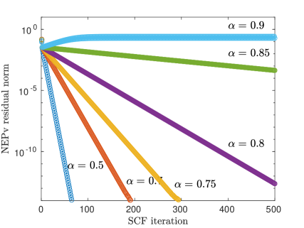
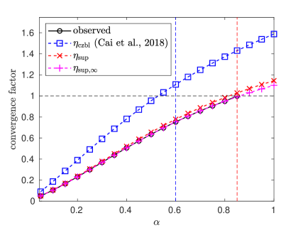
Figure 1: Example 1: convergence history of residual norm $\|H(V_{i})V_{i}-V_{i}\Lambda_{i}\|_{2}$ by the plain SCF (1.3) for selected $\alpha$ (left); and convergence rate estimates as $\alpha$ varies (right).

1. For $\alpha=0$, the NEPv reduces to a standard eigenvalue problem $LV=V\Lambda$, for which SCF converges in one iteration. As $\alpha$ increases, SCF faces increasing challenges to converge. In particular, for $\alpha$ larger than $0.85$, the plain SCF becomes divergent. For those $\alpha$, the “exact” solutions $V_{*}$ used to calculate convergence factors are computed by the level-shifted SCF.

2. The asymptotic average contraction factor $\eta_{\sup,\infty}(=\rho(\mathscr{L}))$ successfully predicts the convergence of SCF in all cases, and perfectly captures the convergence rate. The factor $\eta_{\sup,\infty}$ yields excellent estimation after only a small number of iterative steps, although strictly speaking, it is conclusive only as the iteration number approaches infinity.

3. The contraction factor estimate $\eta_{\sup}$ is an overestimate and usually provides a good prediction of local convergence. It failed slightly at $\alpha=0.85$, where up to 10 digits:

   $$\begin{array}[]{rclrrcl}\mbox{observed}&=&0.9913931781,&\,\,\eta_{\sup,\infty}&=&0.9913931591,\\ \eta_{\sup}&=&1.028434776,&\,\,\eta_{\operatorname{czbl}}&=&1.430511920.\end{array}$$

   The gap between $\eta_{\sup,\infty}$ and $\eta_{\sup}$ implies $\mathscr{L}$ is a non-normal operator as discussed in Section 4.2.

4. In comparison, the estimate $\eta_{\operatorname{czbl}}$ by [4] is less precise. In particular, it fails to correctly indicate the convergence of the plain SCF starting at $\alpha=0.55$, which is in contrast to $\eta_{\sup}$ starting at $0.85$. We mention that, for this same experiment, it was illustrated in [4] that $\eta_{\operatorname{czbl}}<1$ for all $\alpha\leq 0.6$ (marked as dashed vertical line).

Example 2.

In this example, we examine the convergence of the level-shifted SCF (5.1) with respect to the shift $\sigma$. The testing problem is the same as Example 1 but with a fixed $\alpha=1$, for which the plain SCF (1.3) is divergent. We apply the level-shifted SCF with various choices of $\sigma$ for the solution. The convergence history and the corresponding spectral radius of the operator $\mathscr{L}_{\sigma}$ in (5.8) is depicted in Figure 2.

From the spectral radius plot on the right side of Figure 2, we observe that $\rho(\mathscr{L}_{\sigma})$ dropped quickly below $1$. The minimal value $\rho(\mathscr{L}_{\sigma})\approx 0.33$ at $\sigma\approx 0.36$ and leads to rapid convergence of SCF as shown in the left plot. As $\sigma$ grows, $\rho(\mathscr{L}_{\sigma})$ monotonically increases towards 1. Such a behavior of $\rho(\mathscr{L}_{\sigma})$ is consistent with the bound obtained in Theorem 2, governed by rational functions in the form of $|1-a/(\sigma+b)|$ with $a,b>0$.

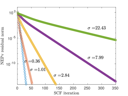
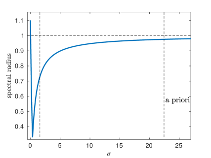
Figure 2: Example 2: convergence history of residual norm $\|H(V_{i})V_{i}-V_{i}\Lambda_{i}\|_{2}$ by the level-shifted SCF (5.1) with selected $\sigma$ (left); spectral radius of $\rho(\mathscr{L}_{\sigma})$ as shift $\sigma$ varies (right), where the first vertical dash line is $\sigma=\frac{\mu_{\max}}{2}-\delta_{*}$ suggested by (5.13) and the second is a-priori $\sigma=\frac{3}{2}\,\alpha\,\|L^{-1}\|_{2}+2$ suggested by (6.7), and the optimal shift is $\sigma\approx 0.36$. The $H(V)$ is given by (6.2) with $\alpha=1$.

The sharp turning of the curve of $\rho(\mathscr{L}_{\sigma})$ reveals the challenge in finding the optimal $\sigma$. The values of spectral radius grows quickly as $\alpha$ moves away from the optimal shift. We note that both the theoretic lower bound in (5.13) and a-priori estimate (6.7) fall correctly into the convergence region. The a-priori bound provided a pessimistic estimate of $\sigma$, that leads to a less satisfactory convergence rate of the level-shifted SCF (5.1).

6.3 Gross–Pitaevskii equation

In this experiment, we consider NEPv with complex coefficient matrices $H(V)$ given by

$$H(V)=A_{f}+\beta\,\operatorname{Diag}(|V|)^{2},$$ (6.8)

where $A_{f}\in\mathbb{C}^{n\times n}$ is a Hermitian matrix and positive definite, $\beta>0$ is a parameter, $V\in\mathbb{C}^{n}$ is a complex vector, and $|\cdot|$ takes elementwise absolute value. Such an NEPv arises from discretizing the Gross-Pitaevskii equation (GPE) for modeling the physical phenomenon of Bose–Einstein condensation [3, 9, 10, 14].

The matrix $A_{f}$ in (6.8) is dependent of a potential function $f$. For illustration, we will discuss a model 2D GPE studied in [9], where for a given potential function $f(x,y)$ over a two dimension domain $[-\ell,\ell]\times[-\ell,\ell]$, the corresponding matrix

$$A_{f}=\operatorname{Diag}(\widetilde{f})-\frac{1}{2}M-\imath\omega M_{\phi},$$ (6.9)

where

$$\widetilde{f}=h^{2}\,\left[f(x_{1},y_{1}),\dots,f(x_{N},y_{1}),f(x_{1},y_{2}),\dots,f(x_{N},y_{2}),\dots,f(x_{N},y_{N})\right]^{\operatorname{T}}\in\mathbb{R}^{N^{2}}$$

with $\{x_{i}\}_{i=1}^{N}$ and $\{y_{i}\}_{i=1}^{N}$ being interior points of the interval $[-\ell,\ell]$ from the $N+2$ equidistant discretization with spacing $h=\frac{2\ell}{N+1}$. The matrices $M$, $M_{\phi}$ are given by

$$M=D_{2,N}\otimes I+I\otimes D_{2,N},\,\,M_{\phi}=h\,\operatorname{Diag}(y_{1},\dots,y_{N})\otimes D_{N}-D_{N}\otimes\left(h\,\operatorname{Diag}(x_{1},\dots,x_{N})\right),$$

with $N\times N$ tridiagonal matrices $D_{N}=\operatorname{tridiag}(-\frac{1}{2},0,\frac{1}{2})$ and $D_{2,N}=\operatorname{tridiag}(1,-2,1)$.

Since $V$ is a vector, by definition (2.11) the directional derivative operator of $H(V)$ is given by

$$\mathbf{D}H(V)[X]=2\beta\,\operatorname{Diag}(\Re(\overline{V}\odot X)).$$

The local $\mathbb{R}$-linear operator of the plain SCF $\mathscr{L}:\mathbb{C}^{n-1}\to\mathbb{C}^{n}$ in (3.8) is

$$\mathscr{L}(Z)=2\beta\,D(V_{*})\odot(V_{*\bot}^{\operatorname{H}}\,\operatorname{Diag}(\Re(\overline{V}_{*}\odot(V_{*\bot}Z)))\,V_{*}),$$ (6.10)

and its adjoint operator $\mathscr{L}^{*}$, with respect to the standard inner product in $\mathbb{C}^{(n-k)\times k}$ ($k=1$), i.e., $\langle\mathscr{L}(Z),Y\rangle\equiv\Re(\operatorname{tr}(Y^{\operatorname{H}}\mathscr{L}(Z)))=\langle Z,\mathscr{L}^{*}(Y)\rangle\equiv\Re(\operatorname{tr}([\mathscr{L}^{*}(Y)]^{\operatorname{H}}Z))$ for any $Y,\,Z\in\mathbb{C}^{(n-k)\times k}$, is given by

$$\mathscr{L}^{*}(Y)=2\beta\,V_{*\bot}^{\operatorname{H}}\,\left(\Re\left(\operatorname{diag}(V_{*\bot}(D(V_{*})\odot Y)V_{*}^{\operatorname{H}})\right)\odot V_{*}\right),$$ (6.11)

see Appendix A for the derivation.

For the level-shifted SCF, the local $\mathbb{R}$-linear operator $\mathscr{L}_{\sigma}$ in (5.8) is given by

$$\mathscr{L}_{\sigma}(Z)=D_{\sigma}(V_{*})\odot\mathscr{Q}(Z)-I_{\rm id},$$ (6.12)

where the restricted derivative operator $\mathscr{Q}(Z)$ is given by

$$\mathscr{Q}(Z)=2\beta\,V_{*\bot}^{\operatorname{H}}\,\operatorname{Diag}(\Re(\overline{V_{*}}\odot(V_{*\bot}Z))\,V_{*}+(\Lambda_{*\bot}Z-Z\Lambda_{*}).$$ (6.13)

The largest eigenvalue $\mu_{\max}$ of $\mathscr{Q}$ can be bounded as follows. Let $Z\in\mathbb{C}^{n-1}$ be the eigenvector associated with $\mu_{\max}$. Then

$$\mu_{\max}=\frac{\|\mathscr{Q}(Z)\|_{\operatorname{F}}}{\|Z\|_{\operatorname{F}}} \leq 2\beta\,\frac{\|\operatorname{Diag}(\Re(\overline{V}\odot(V_{*\bot}Z))\|_{\operatorname{F}}}{\|Z\|_{\operatorname{F}}}+s_{*}$$

$$\leq 2\beta+s_{*}\leq 3\beta+\|A_{f}\|_{2},$$

where $s_{*}=\lambda_{n}(H(V_{*}))-\lambda_{1}(H(V_{*}))$ is the spectral span, and for the last inequality we have used the inequalities $s_{*}\leq\lambda_{n}(H(V_{*}))\leq\beta+\|A_{f}\|_{2}$ due to $H(V)$ in (6.8) being positive definite. Consequently, the lower bound on $\sigma$ in (5.13) yields

$$\sigma\geq\frac{1}{2}(3\beta+\|A_{f}\|_{2})$$ (6.14)

to ensure the local convergence of the level-shifted SCF.

Example 3.

In this example, we select the parameters $\ell=1$, $\omega=0.85$, and $N=10$ (hence $n=100$). We use a radial harmonic potential $f(x,y)=(x^{2}+y^{2})/2$. Various values of $\beta$ ranging from $0.5$ to $5$ have been tried. The simulation results are shown in Figure 3.

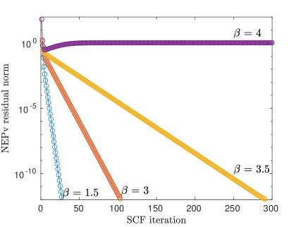
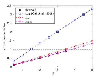
Figure 3: Example 3: (Left) Convergence history of residual norm $\|H(V_{i})V_{i}-V_{i}\Lambda_{i}\|_{2}$ by the plain SCF (1.3) for selected $\beta$; (Right) Convergence rate estimates as $\beta$ varies.

It is observed that the plain SCF becomes slower and slower and eventually divergent as $\beta$ increases. Again, the spectral radius $\rho(\mathscr{L}_{\sigma})$ and $\eta_{\sup}$ can well capture true convergence behavior. In particular, at $\beta=3.5$, we find that up to 7 digits,

$$\mbox{observed}=0.9136140,\quad\eta_{\sup,\infty}=0.9136173,\quad\eta_{\sup}=1.019727,\quad\eta_{\operatorname{czbl}}=2.342686$$

Again, we see the sharpness of the estimate $\eta_{\sup,\infty}$.

The performance of the level-shifted SCF with respect to different shifts $\sigma$ is shown in Figure 4, where we observe a similar convergence behavior to Figure 2 of Example 2 on the impact of the choice of shift $\sigma$.

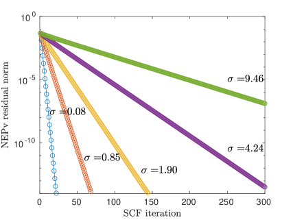
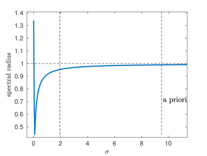
Figure 4: Example 3: convergence history of residual norm $\|H(V_{i})V_{i}-V_{i}\Lambda_{i}\|_{2}$ by the level-shifted SCF (5.1) with selected $\sigma$ (left); spectral radius of $\rho(\mathscr{L}_{\sigma})$ as shift $\sigma$ varies (right), where the first vertical dash line is $\sigma=\frac{\mu_{\max}}{2}-\delta_{*}$ suggested by (5.13) and the second is a-priori $\sigma=\frac{1}{2}(3\beta+\|A_{f}\|_{2})$ suggested by (6.14), and the optimal shift is $\sigma\approx 0.08$. The $H(V)$ is given by (6.8) with $\beta=5$.

Example 4.

This is a repeat of Example 3, except using a non-radical harmonic potential function $f(x,y)=(x^{2}+100y^{2})/2$. The plots in Figure 5 show a slightly different performance of the plain SCF (1.3) compared to the radical harmonic case of Example 3. The sharpness of the estimate $\eta_{\sup,\infty}$ on the local convergence rate can be seen at $\beta=2.2$, where up to 7 digits:

$$\mbox{observed}=0.9652599,\quad\eta_{\sup,\infty}=0.9652614,\quad\eta_{\sup}=1.073434,\quad\eta_{\operatorname{czbl}}=2.043247$$

The performance of the level-shifted SCF is depicted in Figure 6. Again we observe a similar convergence behavior to Example 3 with repect to the choice of shift $\sigma$.

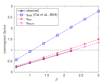
Figure 5: Example 4: convergence history of residual norm $\|H(V_{i})V_{i}-V_{i}\Lambda_{i}\|_{2}$ by the plain SCF (1.3) for selected $\beta$ (left); convergence rate estimates as $\beta$ varies (right).

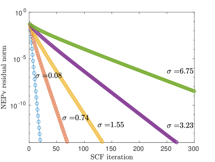
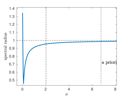
Figure 6: Example 4: convergence history of residual norm $\|H(V_{i})V_{i}-V_{i}\Lambda_{i}\|_{2}$ by the level-shifted SCF (5.1) with selected $\sigma$ (left); spectral radius of $\rho(\mathscr{L}_{\sigma})$ as shift $\sigma$ varies (right), where the first vertical dash line is $\sigma=\frac{\mu_{\max}}{2}-\delta_{*}$ suggested by (5.13) and the second is a-priori $\sigma=\frac{1}{2}(3\beta+\|A_{f}\|_{2})$ suggested by (6.14), and the optimal shift is $\sigma\approx 0.08$. The $H(V)$ is given by (6.8) with $\beta=3$.

7 Concluding remarks

We have presented a comprehensive local convergence analysis of the plain SCF iteration and its level-shifted variant for solving NEPv. The optimal convergence rate and estimates are established. Our analysis is in terms of the tangent-angle matrix to measure the approximation error between consecutive SCF iterates and the intended target. We first established a relation between the tangent-angle matrices associated with any two consecutive SCF approximates, and with it we developed new formulas for the local error contraction factor and the asymptotic average contraction factor of SCF. The new formulas are sharper and complement previously established local convergence results. With the help of new convergence rate estimates, we derive an explicit lower-bound on the shifting parameter to guarantee local convergence of the level-shifted SCF. These results are numerically confirmed by examples from applications in computational physics and chemistry.

Our analysis does not cover more sophisticated variants of SCF such as the damped SCF [5] and the Direct Inversion of Iterative Subspace (DIIS) [23, 24]. It is conceivable that by the tangent-angle matrix and the eigenspace perturbation theory, one can pursue the local convergence analysis of those variants.

Finally, we note that we focused on NEPv (1.1) satisfying the invariant property (1.2). While this property is formulated as a result of some practically important applications, there are recent emerging NEPv (1.1) that do not have this property, such as the one in [40], and yet similar SCF iterations can be used. It would be interesting to find out what now determines the optimal local convergence rate. This will be a future project to pursue.

Appendix A Adjoint operators

The adjoint $\mathscr{L}^{*}$ in (6.4) is derived as follows.

$$\langle\,Y,\mathscr{L}(Z)\,\rangle =2\alpha\,\langle\,Y,\,\,D(V_{*})\odot(V_{*\bot}^{\operatorname{T}}\,\operatorname{Diag}(L^{-1}\operatorname{diag}(V_{*\bot}ZV_{*}^{\operatorname{T}}))\,V_{*})\,\rangle$$

(1) by $$\langle Y,D\odot X\rangle=\langle D\odot Y,X\rangle =2\alpha\,\langle\,D(V_{*})\odot Y,\,\,V_{*\bot}^{\operatorname{T}}\,\operatorname{Diag}(L^{-1}\operatorname{diag}(V_{*\bot}ZV_{*}^{\operatorname{T}}))\,V_{*}\,\rangle$$

(2) by $$\langle Y,AXB\rangle=\langle A^{\operatorname{T}}YB^{\operatorname{T}},X\rangle =2\alpha\,\langle\,V_{*\bot}[D(V_{*})\odot Y]V_{*}^{\operatorname{T}},\,\,\operatorname{Diag}(L^{-1}\operatorname{diag}(V_{*\bot}ZV_{*}^{\operatorname{T}}))\,\rangle$$

(3) by $$\langle Y,\operatorname{Diag}(b)\rangle=\langle\operatorname{diag}(Y),b\rangle =2\alpha\,\langle\,\operatorname{diag}(V_{*\bot}[D(V_{*})\odot Y]V_{*}^{\operatorname{T}}),\,\,L^{-1}\operatorname{diag}(V_{*\bot}ZV_{*}^{\operatorname{T}})\,\rangle$$

(4) by moving $$L =2\alpha\,\langle\,L^{-1}\operatorname{diag}(V_{*\bot}[D(V_{*})\odot Y]V_{*}^{\operatorname{T}}),\,\,\operatorname{diag}(V_{*\bot}ZV_{*}^{\operatorname{T}})\,\rangle$$ to the left

(5) by $$\langle\operatorname{Diag}(b),Y\rangle=\langle b,\operatorname{diag}(Y)\rangle =2\alpha\,\langle\,\operatorname{Diag}(L^{-1}\operatorname{diag}(V_{*\bot}[D(V_{*})\odot Y]V_{*}^{\operatorname{T}})),\,\,V_{*\bot}ZV_{*}^{\operatorname{T}}\,\rangle.$$

Finally, moving $V_{*\bot}$ and $V_{*}$ to the left we obtain the formula (6.4).

The adjoint $\mathscr{L}^{*}$ in (6.11) is derived analogously. The first three steps are exactly the same as above, and so we continue with

$$\langle\,Y,\mathscr{L}(Z)\,\rangle =2\beta\,\langle\,Y,\,\,D(V_{*})\odot(V_{*\bot}^{\operatorname{H}}\,\operatorname{Diag}(\Re(\overline{V}_{*}\odot(V_{*\bot}Z)))\,V_{*})\,\rangle$$

by (1)–(3) above $$=2\beta\,\langle\,\operatorname{diag}(V_{*\bot}[D(V_{*})\odot Y]V_{*}^{\operatorname{H}}),\,\,\Re(\overline{V}_{*}\odot(V_{*\bot}Z))\,\rangle$$

since it’s vector inner product $$=2\beta\,\langle\,\Re(\operatorname{diag}(V_{*\bot}[D(V_{*})\odot Y]V_{*}^{\operatorname{H}})),\,\,\overline{V}_{*}\odot(V_{*\bot}Z)\,\rangle$$

by $$\langle Y,\operatorname{Diag}(b)\rangle=\langle\operatorname{diag}(Y),b\rangle =2\beta\,\langle\,\Re(\operatorname{diag}(V_{*\bot}[D(V_{*})\odot Y]V_{*}^{\operatorname{H}}))\odot{V}_{*},\,\,V_{*\bot}Z\,\rangle.$$

Finally, moving $V_{*\bot}$ to the left, we obtain the formula (6.11).

References

- [1] Z. Bai, D. Lu, and B. Vandereycken. Robust Rayleigh quotient minimization and nonlinear eigenvalue problems. SIAM J. Sci. Comput., 40(5):A3495–A3522, 2018.
- [2] W. Bao and Y. Cai. Mathematical theory and numerical methods for Bose-Einstein condensation. Kinetic & Related Models, 6(1), 2013.
- [3] W. Bao and Q. Du. Computing the ground state solution of Bose–Einstein condensates by a normalized gradient flow. SIAM J. Sci. Comput., 25(5):1674–1697, 2004.
- [4] Y. Cai, L.-H. Zhang, Z. Bai, and R.-C. Li. On an eigenvector-dependent nonlinear eigenvalue problem. SIAM J. Matrix Anal. Appl., 39(3):1360–1382, 2018.
- [5] E. Cancès and C. Le Bris. Can we outperform the DIIS approach for electronic structure calculations? Int. J. Quantum Chem., 79(2):82–90, 2000.
- [6] E. Cancès and C. Le Bris. On the convergence of scf algorithms for the Hartree–Fock equations. ESAIM: Mathematical Modelling and Numerical Analysis, 34(4):749–774, 2000.
- [7] C. Davis and W. M. Kahan. The rotation of eigenvectors by a perturbation. III. SIAM J. Numer. Anal., 7(1):1–46, 1970.
- [8] J. W. Demmel. Applied Numerical Linear Algebra. SIAM, 1997.
- [9] E. Jarlebring, S. Kvaal, and W. Michiels. An inverse iteration method for eigenvalue problems with eigenvector nonlinearities. SIAM J. Sci. Comput., 36(4):A1978–A2001, 2014.
- [10] S. Jia, H. Xie, M. Xie, and F. Xu. A full multigrid method for nonlinear eigenvalue problems. Sci. China Math., 59(10):2037–2048, 2016.
- [11] L. Jost, S. Setzer, and M. Hein. Nonlinear eigenproblems in data analysis: Balanced graph cuts and the ratioDCA-Prox. In Extraction of quantifiable information from complex systems, pages 263–279. Springer, 2014.
- [12] J. Kouteckỳ and V. Bonačić. On convergence difficulties in the iterative Hartree—Fock procedure. J. Chem. Phys., 55(5):2408–2413, 1971.
- [13] P.D. Lax. Functional Analysis. Wiley, 2002.
- [14] X.-G. Li, Y. Cai, and P. Wang. Operator-compensation methods with mass and energy conservation for solving the Gross-Pitaevskii equation. Applied Numerical Mathematics, 151:337–353, 2020.
- [15] X. Liu, X. Wang, Z. Wen, and Y. Yuan. On the convergence of the self-consistent field iteration in Kohn-Sham density functional theory. SIAM J. Matrix Anal. Appl., 35(2):546–558, 2014.
- [16] X. Liu, Z. Wen, X. Wang, and Y. Ulbrich, M. Yuan. On the analysis of the discretized kohn-Sham density functional theory. SIAM J. Numer. Anal., 53(4):1758–1785, 2015.
- [17] R. M. Martin. Electronic structure: basic theory and practical methods. Cambridge university press, 2004.
- [18] R. McWeeny. Some recent advances in density matrix theory. Reviews of Modern Physics, 32(2):335, 1960.
- [19] R. Meyer. Nonlinear eigenvector algorithms for local optimization in multivariate data analysis. Linear Algebra Its Appl., 264:225–246, 1997.
- [20] T. T. Ngo, M. Bellalij, and Y. Saad. The trace ratio optimization problem. SIAM review, 54(3):545–569, 2012.
- [21] J. Nocedal and S. Wright. Numerical optimization. Springer Science & Business Media, 2006.
- [22] B. N. Parlett. The symmetric eigenvalue problem. SIAM, 1998.
- [23] P. Pulay. Convergence acceleration of iterative sequences. the case of SCF iteration. Chem. Phys. Lett., 73(2):393–398, 1980.
- [24] Peter Pulay. Improved SCF convergence acceleration. J. Comput. Chem., 3(4):556–560, 1982.
- [25] L. Qiu, Y. Zhang, and C.-K. Li. Unitarily invariant metrics on the Grassmann space. SIAM J Matrix Anal. Appl., 27(2):507–531, 2005.
- [26] C. C. J. Roothaan. New developments in molecular orbital theory. Rev. Mod. Phys., 23(2):69, 1951.
- [27] V.R. Saunders and I.H. Hillier. A Level–Shifting method for converging closed shell Hartree–Fock wave functions. Int. J. Quantum Chem., 7(4):699–705, 1973.
- [28] R. E. Stanton. The existence and cure of intrinsic divergence in closed shell SCF calculations. J. of Chem. Phys., 75(7):3426–3432, 1981.
- [29] R. E. Stanton. Intrinsic convergence in closed-shell SCF calculations. A general criterion. J. Chem. Phys., 75(11):5416–5422, 1981.
- [30] G. W. Stewart. Matrix Algorithms: Volume II: Eigensystems. SIAM, 2001.
- [31] G. W. Stewart and J. G. Sun. Matrix Perturbation Theory. Academic Press, 1990.
- [32] A. Szabo and N. S. Ostlund. Modern Quantum Chemistry: Introduction To Advanced Electronic Structure Theory. Courier Corporation, 2012.
- [33] L. Thøgersen, J. Olsen, D. Yeager, P. Jørgensen, P. Sałek, and T. Helgaker. The trust-region self-consistent field method: Towards a black-box optimization in Hartree–Fock and Kohn–Sham theories. J Chem. Phys., 121(1):16–27, 2004.
- [34] F. Tudisco and D. J. Higham. A nonlinear spectral method for core-periphery detection in networks. SIAM J. Math. Data Science, 1(2):269–292, 2019.
- [35] P. Upadhyaya, E. Jarlebring, and E. H. Rubensson. A density matrix approach to the convergence of the self-consistent field iteration. arXiv preprint arXiv:1809.02183, 2018.
- [36] R. S. Varga. Matrix Iterative Analysis. Springer-Verlag, Berlin, 2000.
- [37] C. Yang, W. Gao, and J. C. Meza. On the convergence of the self-consistent field iteration for a class of nonlinear eigenvalue problems. SIAM J. Matrix Anal. Appl., 30(4):1773–1788, 2009.
- [38] C. Yang, J. C. Meza, and L.-W. Wang. A trust region direct constrained minimization algorithm for the Kohn–Sham equation. SIAM J. Sci. Comput., 29(5):1854–1875, 2007.
- [39] L. Zhang and R.-C. Li. Maximization of the sum of the trace ratio on the Stiefel manifold, I: Theory. Sci. China Math., 57(12):2495–2508, 2014.
- [40] L. Zhang, L. Wang, Z. Bai, and R.-C. Li. A self-consistent-field iteration for orthogonal canonical correlation analysis. IEEE Trans. Pattern Anal. Mach. Intell., 2020. to appear.
- [41] Z. Zhao, Z.-J. Bai, and X.-Q. Jin. A Riemannian Newton algorithm for nonlinear eigenvalue problems. SIAM J. Matrix Anal. Appl., 36(2):752–774, 2015.
- [42] P. Zhu and A. V. Knyazev. Angles between subspaces and their tangents. J. Numer. Math., 21(4):325–340, 2013.