Thermal and IR Drop Analysis Using
Convolutional Encoder-Decoder Networks

Abstract

Computationally expensive temperature and power grid analyses are required during the design cycle to guide IC design. This paper employs encoder-decoder based generative (EDGe) networks to map these analyses to fast and accurate image-to-image and sequence-to-sequence translation tasks. The network takes a power map as input and outputs the corresponding temperature or IR drop map. We propose two networks: (i) ThermEDGe: a static and dynamic full-chip temperature estimator and (ii) IREDGe: a full-chip static IR drop predictor based on input power, power grid distribution, and power pad distribution patterns. The models are design-independent and must be trained just once for a particular technology and packaging solution. ThermEDGe and IREDGe are demonstrated to rapidly predict on-chip temperature and IR drop contours in milliseconds (in contrast with commercial tools that require several hours or more) and provide an average error of 0.6% and 0.008% respectively.

I Introduction

One of the major challenges faced by an advanced-technology node IC designer is the overhead of large run-times of analysis tools. Fast and accurate analysis tools that aid quick design turn-around are particularly important for two critical, time-consuming simulations that are performed several times during the design cycle:

• Thermal analysis, which checks the feasibility of a placement/floorplan solution by computing on-chip temperature distributions in order to check for temperature hot spots.

• IR drop analysis in power distribution networks (PDNs), which diagnoses the goodness of the PDN by determining voltage (IR) drops from the power pads to the gates.

The underlying computational engines that form the crux of both analyses are similar: both simulate networks of conductances and current/voltage sources by solving a large system of equations of the form $G{\bf V}={\bf J}$ [1, 2] with millions to billions of variables. In modern industry designs, a single full-chip temperature or IR drop simulation can take hours to several hours. Accelerating these analyses opens the door to optimizations in the design cycle that iteratively invoke these engines under the hood.

The advent of machine learning (ML) has presented fast and fairly accurate solutions to these problems [3, 4, 5, 6, 7, 8] which can successfully be used in early design cycle optimizations, operating within larger allowable error margins at these stages. To the best of our knowledge, no published work addresses full-chip ML-based thermal analysis: the existing literature focuses on coarser-level thermal modeling at the system level [3, 4, 5]. For PDN analysis, the works in [6, 7] address incremental analysis, and are not intended for full-chip estimation. The work in [8] proposes a convolutional neural network (CNN)-based implementation for full-chip IR drop prediction, using cell-level power maps as features. However, it assumes similar resistance from each cell to the power pads, which may not be valid for practical power grids with irregular grid density. The analysis divides the chip into regions (tiles), and the CNN operates on each tile and its near neighbors. Selecting an appropriate tile and window size is nontrivial – small windows could violate the principle of locality [9], causing inaccuracies, while large windows could result in large models with significant runtimes for training and inference. Our approach bypasses window size selection by providing the entire power map as a feature, allowing ML to learn the window size for accurate estimation.

We translate static analysis problems to an image-to-image translation task and dynamic analysis problems to video-to-video translation, where the inputs are the power/current distributions and the required outputs are the temperature or IR drop contours. For static analysis, we employ fully convolutional (FC) EDGe networks for rapid and accurate thermal and IR drop analysis. FC EDGe networks have proven to be very successful with image-related problems with 2-D spatially distributed data [10, 11, 12, 13] when compared to other networks that operate without spatial correlation awareness. For transient analysis, we use long-short-term-memory (LSTM) based EDGe networks that maintain memory of analyses at prior time steps.

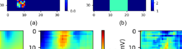
Figure 1: Image-to-image translation using EDGe network.

Based on these concepts, this work proposes two novel ML-based analyzers: ThermEDGe for both full-chip static and transient thermal analysis, and IREDGe for full-chip static IR drop estimation. The fast inference times of ThermEDGe and IREDGe enable full-chip thermal and IR drop analysis in milliseconds, as opposed to runtimes of several hours using commercial tools. We obtain average error of 0.6% and 0.008% for ThermEDGe and IREDGe, respectively, over a range of testcases. We will open-source our software.

Fig. 1 shows a general top-level structure of an EDGe network. It consists of two parts: (i) the encoder/downsampling path, which captures global features of the 2-D distributions of power dissipation, and produces a low-dimensional state space and (ii) the decoder/upsampling path, which transforms the state space into the required detailed outputs (temperature or IR drop contours). The EDGe network is well-suited for PDN/thermal analyses because:
(a) The convolutional nature of the encoder captures the dependence of both problems on the spatial distributions of power. Unlike CNNs, EDGe networks contain a decoder which acts as a generator to convert the extracted power and PDN density features into accurate high-dimensional temperature and IR drop contours across the chip.
(b) The trained EDGe network model for static analysis is chip-area-independent: it only stores the weights of the convolutional kernel, and the same filter can be applied to a chip of any size. The selection of the network topology (convolution filter size, number of convolution layers) is related to the expected sizes of the hotspots rather than the size of the chip: these sizes are generally similar for a given application domain, technology, and packaging choice.
(c) Unlike prior methods [8] that operate tile-by-tile, where finding the right tile and window size for accurate analysis is challenging, the choice of window size is treated as an ML hyperparameter tuning problem to decide the necessary amount of input spatial information.

II EDGe Network for PDN and Thermal Analysis

II-A Problem formulations and data representation

This section presents the ML-based framework for ThermEDGe and IREDGe. The first step is to extract an appropriate set of features from a standard design-flow environment. The layout database provides the locations of each instance and block in the layout, as outlined in Fig. 2(a). This may be combined with information from a power analysis tool such as [14] (Fig. 2(b)) that is used to build a 2-D spatial power map over the die area.

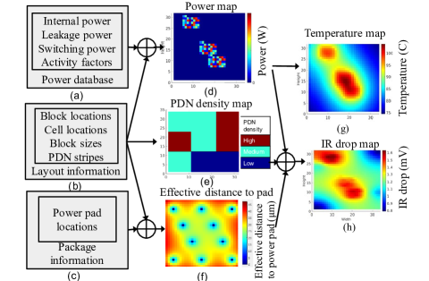
Figure 2: Data representation: Mapping PDN and thermal analysis problems into image-to-image translations tasks.

For thermal analysis using ThermEDGe, both the inputs and outputs are images for the static case, and a sequence of images for the transient case. Each input image shows a 2-D die power distribution (static) image, and each output image is a temperature map across the die (Fig. 2). For static PDN analysis, the output is an IR drop map across the full chip. However, in addition to the 2-D power distributions, IREDGe has two other inputs:

(i) A PDN density map: This feature is generated by extracting the average PDN pitch in each region of the chip. For example, when used in conjunction with the PDN styles in [15, 16], where the chip uses regionwise uniform PDNs, the average PDN density in each region, across all metal layers, is provided as an input (Fig. 2(e)).

(ii) An effective distance to power pad: This feature represents the equivalent distance from an instance to all power pads in the package. We compute the effective distance of each instance, $d_{e}$, to $N$ power pads on the chip as the harmonic sum of the distances to the pads:

$$d_{e}^{-1}=d_{1}^{-1}+d_{2}^{-1}+...+d_{N}^{-1}$$ (1)

where $d_{i}$ is the distance of the $i^{th}$ power pad from the instance. Intuitively, the effective distance metric and the PDN density map together, represent the equivalent resistance between the instance and the pad. The equivalent resistance is a parallel combination of each path from the instance to the pad. We use distance to each pad as a proxy for the resistance in Eq. (1). Fig. 2(f) shows a typical “checkerboard” power pad layout for flip-chip packages [17, 18].

Temperature depends on the ability of the package and system to conduct heat to the ambient, and IR drop depends on off-chip (e.g., package) parasitics. In this work, our focus is strictly on-chip, and both ThermEDGe and IR-EDGe are trained for fixed models of a given technology, package, and system.

Next, we map these problems to standard ML networks:

• For static analysis, the problem formulations require a translation from an input power image to an output image, both corresponding to contour maps over the same die area, and we employ a U-Net-based EDGe network [11].

• The dynamic analysis problem requires the conversion of a sequence of input power images, to a sequence of output images of temperature contours, and this problem is addressed using an LSTM-based EDGe network [19].

We describe these networks in the rest of this section.

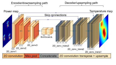
Figure 3: U-Net-based EDGe network for static thermal and PDN analysis.

II-B U-Nets for static thermal and PDN analysis

II-B1 Overview of U-Nets

CNNs are successful in extracting 2-D spatial information for image classification and image labeling tasks, which have low-dimensional outputs (class or label). For PDN and thermal analysis tasks, the required outputs are high-dimensional distributions of IR drop and temperature contour, where the dimensionality corresponds to the number of pixels of the image and the number of pixels is proportional to the size of the chip. This calls for a generator network that can translate the extracted low-dimensional power and PDN features from a CNN-like encoder back into high-dimensional representing the required output data.

Fig. 3 shows the structure of the EDGe network used for static PDN and thermal analysis. At the top level, it consists of two networks:

(a) Encoder/downsampling network Like a CNN, the network utilizes a sequence of 2-D convolution and max pooling layer pairs that extract key features from the high-dimensional input feature set. The convolution operation performs a weighted sum on a sliding window across the image [20], and the max pooling layer reduces the dimension of the input data by extracting the maximum value from a sliding window across the input image. In Fig. 3, the feature dimension is halved at each stage by each layer pair, and after several such operations, an encoded, low-dimensional, compressed representation of the input data is obtained. For this reason, the encoder is also called the downsampling path: intuitively, downsampling helps understand the “what” (e.g., “Does the image contain power or IR hotspots?”) in the input image but tends to be imprecise with the “where” information (e.g., the precise locations of the hotspots). The latter is recovered by the decoder stages.

(b) Decoder/upsampling network Intuitively, the generative decoder is responsible for retrieving the “where” information that was lost during downsampling, This distinguishes an EDGe network from its CNN counterpart. The decoder is implemented using the transpose convolution [20] and upsampling layers. Upsampling layers are functionally the opposite of a pooling layer, and increase the dimension of the input data matrix by replicating the rows and columns.

II-B2 Use of skip connections

Static IR drop and temperature are strongly correlated to the input power – a region with high power on the chip could potentially have an IR or temperature hotspot in its vicinity. U-Nets [11] utilize skip connections between the downsampling and upsampling paths, as shown in Fig. 3. These connections take information from one layer and incorporate it using a concatenation layer at a deeper stage skipping intermediate layers, and appends it to the embedding along the z-dimension.

For IR analysis, skip connections combine the local power, PDN information, and power pad locations from the downsampling path with the global power information from the upsampling path, allowing the underlying input features to and directly shuttle to the layers closer to the output, and are similarly helpful for thermal analysis. This helps recover the fine-grained (“where”) details that are lost in the encoding part of the network (as stated before) during upsampling in the decoder for detailed temperature and IR drop contours.

II-B3 Receptive fields in the encoder and decoder networks

The characteristic of PDN and thermal analyses problems is that the IR drop and temperature at each location depend on both the local and global power information. During convolution, by sliding averaging windows of an appropriate size across the input power image, the network captures local spatially correlated distributions. For capturing the larger global impact of power on temperature and IR drop, max pooling layers are used after each convolution to appropriately increase the size of the receptive field at each stage of the network. The receptive field is defined as the region in the input 2-D space that affects a particular pixel, and it determines the impact of the local, neighboring, and global features on PDN and thermal analysis.

In a deep network, the value of each pixel feature is affected by all of the other pixels in the receptive field at the previous convolution stage, with the largest contributions coming from pixels near the center of the receptive field. Thus, each feature not only captures its receptive field in the input image, but also gives an exponentially higher weight to the middle of that region [21]. This matches with our applications, where both thermal and IR maps for a pixel are most affected by the features in the same pixel, and partially by features in nearby pixels, with decreasing importance for those that are farther away. The size of the receptive field at each stage in the network is determined by the convolutional filter size, number of convolutional layers, max pooling filter sizes, and number of max pooling layers.

On both the encoder and decoder sides in Fig. 3, we use three stacked convolution layers, each followed by 2$\times$2 max-pooling to extract the features from the power and PDN density images. The number of layers and filter sizes are determined based on the magnitude of the hotspot size encountered during design iterations.

II-C LSTM-based EDGe network for transient thermal analysis

Long short term memory (LSTM) based EDGe networks are a special kind of recurrent neural network (RNN) that are known to be capable of learning long term dependencies in data sequences, i.e., they have a memory component and are capable of learning from past information in the sequence.

Figure 4: LSTM-based EDGe network for transient analysis in ThermEDGe.

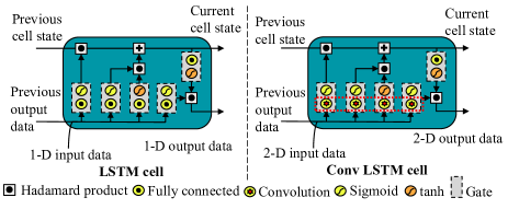
Figure 5: A fully connected LSTM cell (left) and a ConvLSTM cell (right).

For transient thermal analysis, the structure of ThermEDGe is shown in Fig. 4. The core architecture is an EDGe network, similar to the static analysis problem described in Section II-B, except that the network uses additional LSTM cells to account for the time-varying component. The figure demonstrates the time-unrolled LSTM where input power frames are passed to the network one frame at a time. The LSTM cell accounts for the history of the power maps to generate the output temperature frames for all time steps. The network is used for sequence-to-sequence translation in transient thermal analysis, where the input is a set of time-varying power maps and the output is a set of time-varying temperature maps (Section II-A).

Similar to the static ThermEDGe network (Fig. 3), the encoder consists of convolution and max pooling layers to downsample and extract critical local and global spatial information and the decoder consists of upsampling and transpose convolution layers to upsample the encoded output. However, in addition, transient ThermEDGe has LSTM layers in both the encoding and decoding paths.

A standard LSTM cell is shown in Fig. 5 (left). While the basic LSTM cell uses fully connected layers within each gate, our application uses a variation of an LSTM cell called a convolutional LSTM (ConvLSTM) [22], shown in Fig. 5 (right). In this cell, the fully connected layers in each gate are replaced by convolution layers that capture spatial information. Thus, the LSTM-based EDGe network obtains a spatiotemporal view that enables accurate inference.

III ThermEDGe and IREDGe Model Training

We train the models that go into ThermEDGe and IREDGe to learn the temperature and IR contours from the “golden” commercial tool-generated or ground truth data. We train ThermEdge using the full physics-based thermal simulations from the Ansys-Icepak [23] simulator, incorporating off-chip thermal dynamics from package and system thermal characteristics. IREDGe is trained using static IR drop distribution from a PDN analyzer [24, 14] for various power, PDN density, and power pad distributions.

III-A Generating training data

Static ThermEDGe and IREDGe A challenge we faced to evaluate our experiments is the dearth of public domain benchmarks that fit these applications. The IBM benchmarks [25], are potential candidates for our applications, but they assume constant currents per region and represent an older technology node. Therefore, we generate our dataset which comprises of 50 industry-relevant testcases, where each testcase represents industry-standard workloads for commercial designs implemented in a FinFET technology. The power images of size 34$\times$32 pixels, with each pixel representing the power/temperature a 250$\mu$m$\times$250$\mu$m tile on an 8.5mm$\times$8mm chip. Our training is specific to the resolution: for another image resolution, the model must be retrained. We reiterate that although the training is performed on chips of fixed size, as we show (Section IV), inference can be performed on a chip of any size as long as the resolution remains the same.

For static ThermEDGe our training data is based on static Ansys-Icepak [23] simulations of these 50 testcases. For IREDGe, we synthesize irregular PDNs of varying densities for each dataset element using PDN templates, as defined by OpeNPDN [16]. These templates are a set of PDN building blocks, spanning multiple metal layers in a 14nm commercial FinFET technology, which vary in their metal utilization. For our testcases, we use three templates (high, medium, and low density) and divide the chip into nine regions. As outlined in Section II-A), we use a checkerboard pattern of power pads that vary in the bump pitch and offsets across the dataset.

The synthesized full-chip PDN, power pad locations, and power distributions are taken as inputs into the IR analyzer [24] to obtain training data for IREDGe. For each of the 50 testcases, we synthesize 10 patterns of PDN densities, and for each combination of combination of power and PDN distribution we synthesize 10 patterns of power pad distributions, creating a dataset with 5000 points.

Transient ThermEDGe For the transient analysis problem, our training data is based on transient Ansys-Icepak [23] simulations. The size of the chip is the same as that of the static ThermEDGe testcases. For each testcase, we generate 45 time-step simulations that range from 0 to 3000s, with irregular time intervals from the thermal simulator. Each simulation is expensive in terms of the time and memory resources: one simulation of a 3000s time interval with 45 time-steps can take 4 hours with 2 million nodes. Transient ThermEDGe is trained using constant time steps of 15s which enables easy integration with existing LSTM architectures which have an implicit assumption of uniformly distributed time steps, without requiring additional features to account for the time. The model is trained on 150 testcases with time-varying workloads as features, and their time-varying temperature from Ansys-Icepak as labels.

III-B Model training

For the static analysis problem, ThermEDGe and IREDGe use a static power map as input and PDN density map (for IR analysis only) to predict the corresponding temperature and IR drop contours. For the transient thermal analysis problem, the input is a sequence of 200 power maps and the output is a sequence of 200 temperature contours maps at a 15s time interval. The ML model and training hyperparameters used for these models are listed in Table I.

TABLE I: ThermEDGe and IREDGe ML hyperparameters

ML hyperparameters			Static ThermEDGe	IREDGe	Transient ThermEDGe
Model layer parameters	2D_conv1 2D_conv_trans1	filter size	5x5	3x3	5x5
		# filters	64	64	64
	2D_conv2 2D_conv_trans2	filter size	3x3	3x3	3x3
		# filters	32	32	32
	2D_conv3 2D_conv_trans3	filter size	3x3	3x3	–
		# filters	16	16	–
	Max pool layers	filter size	2x2	2x2	2x2
	ConvLSTM	filter size	–	–	7x7
		# filters	–	–	16
Training parameters	Epochs		500
	Optimizer		ADAM
	Loss function		Pixelwise MSE
	Decay rate		0.98
	Decap steps		1000
	Regularizer		L2
	Regularization rate		1.00E-05
	Learning rate		1.00E-03

We split the data in each set, using 80% of the data points for training, 10% for test, and 10% for validation. The training dataset is normalized by subtracting the mean and dividing by the standard deviation. The normalized golden dataset is used to train the network using an ADAM optimizer [26] where the loss function is a pixel-wise mean square error (MSE). The convolutional operation in the encoder and the transpose convolution in the decoder are each followed by ReLU activation to add non-linearity and L2 regularization to prevent over fitting. The model is trained in Tensorflow 2.1 on an NVIDIA GeForce RTX2080Ti GPU. Training run-times are: 30m each for static ThermEDGe and IREDGe, and 6.5h for transient ThermEDGe. We reiterate that this is a one-time cost for a given technology node and package, and this cost is amortized over repeated use over many design iterations for multiple chips.

IV Results and Analysis using TherEDGe/IREDGe

IV-A Experimental setup and metric definitions

ThermEDGe and IREDGe are implemented using Python3.7 within a Tensorflow 2.1 framework. We test the performance of our models on the 10% of datapoints reserved for the testset (Section III-B) which are labeled T1–T21. As mentioned earlier in Section III-A, due the unavailability of new, public domain benchmarks to evaluate our experiments, we use benchmarks that represent commercial industry-standard design workloads.

Error metrics As a measure of goodness of ThermEDGe and IREDGe predictions, we define a discretized regionwise error, $T_{err}~{}=~{}\left|T_{true}-T_{pred}\right|$, where $T_{true}$ is ground truth image, generated by commercial tools, and $T_{pred}$ the predicted image, generated by ThermEDGe. $IR_{err}$ is computed in a similar way. We report the average and maximum values of $T_{err}$ and $IR_{err}$ for each testcase. In addition, the percentage mean and maximum error are listed as a fraction of a temperature corner, i.e., 105^∘C for thermal analysis and as a fraction of VDD$=0.7$V for IR drop analysis.

IV-B Performance of ThermEDGe and IREDGe: Accuracy and speed

Static ThermEDGe results A comparison between the commercial tool-generated temperature and the ThermEDGe-generated temperature map for T1–T5 are listed in Table II. The runtime of static ThermEDGe for each the five testcases which are of size 34$\times$32 is approximately 1.1ms in our environment. On average across the five testcases (five rows of the table), ThermEDGe has an average $T_{err}$ of 0.63^∘C and a maximum $T_{err}$ of 2.93^∘C. These numbers are a small fraction when compared to the maximum ground truth temperature of these testcases (85 – 150^∘C). The fast runtimes imply that our method can be used in the inner loop of a thermal optimizer, e.g., to evaluate various chip configurations under the same packaging solution (typically chosen early in the design process). For such applications, this level of error is very acceptable.

TABLE II: Summary of ThermEDGe results for static and transient analysis across 10 testcases.

Static ThermEDGe			Transient ThermEDGe
#Testcase	Avg. $\bf T_{err}$	Max $\bf T_{err}$	#Testcase	Avg. $\bf T_{err}$	Max $\bf T_{err}$
T1	0.64C (0.61%)	2.76C (2.63%)	T6	0.51C (0.49%)	5.59C (5.32%)
T2	0.63C (0.60%)	2.67C (2.54%)	T7	0.58C (0.55%)	6.17C (5.88%)
T3	0.65C (0.62%)	2.93C (2.79%)	T8	0.57C (0.54%)	5.83C (5.55%)
T4	0.48C (0.46%)	2.22C (2.11%)	T9	0.52C (0.50%)	6.32C (6.02%)
T5	0.75C (0.71%)	2.86C (2.72%)	T10	0.56C (0.53%)	7.14C (6.80%)

Figure 6: ThermEDGe static temperature estimation on T1: (a) input normalized power distribution, (b) histogram of $T_{err}$ where maximum error is 2.76^∘C which is very small compared to the maximum temperature of 85^∘C, (c) ground truth temperature map, and (d) predicted temperature map.

A graphical view of the predicted map for T1 is depicted in Fig. 6. For a given input power distribution in Fig. 6(a), ThermEDGe generates the temperature contour plots, as shown in Fig. 6(d). We compare the predicted value against the true value (Fig. 6(c)). The discrepancy is visually seen to be small. Numerically, the histogram in Fig. 6(b) shows the distribution of %$T_{err}$ across regions (Fig. 6(b). The average $T_{err}$ 0.64^∘C and the maximum $T_{err}$ is 2.93^∘C. This corresponds an average error of 0.52% and worst-case error of 2.79% as shown in the figure.

Transient ThermEDGe results The transient thermal analysis problem is a sequence-to-sequence prediction task where each datapoint in the testset has 200 frames of power maps at a 15s interval. Trained transient ThermEDGe predicts the output temperature sequence for the input power sequence. We summarize the results in Table II. The inference run-times of T6–10 to generate a sequence 200 frames of temperature contours is approximately 10ms in our setup. Across the five testcases, the prediction has an average $T_{err}$ of 0.52% and a maximum $T_{err}$ of 6.80% as shown. The maximum $T_{err}$ in our testcases occur during transients which do not have long-last effects (e.g., on IC reliability). These errors are reduced to the average $T_{err}$ values at sustained peak temperatures.

Fig. 7 (left) shows an animated video of the time-varying power map for T6, where each frame (time-step) is after a 15s time interval. As before, the corresponding ground truth and predicted temperature contours are depicted in center and right, respectively, of the figure.

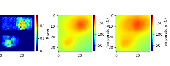
Figure 7: [For an animated version, visit the GitHub repository: https://github.com/asp-dac/asp-dac-1323.git to view the video.] Video comparing the prediction of transient ThermEDGe against commercial tool-generated temperature contours for T6: (i) left video shows the time-varying power map, (ii) center video shows the commercial tool-generated temperature maps, and (iii) right video shows ThermEDGe-generated temperature maps

IREDGe results We compare IREDGe-generated contours against the contours generated by  [24] across 500 different testcases (10% of the data, orthogonal to the training set) with varying PDN densities and power distributions. Across the five testcases in Table III, IREDGe has an average $IR_{err}$ of 0.053mV and a worstcase max $IR_{err}$ of 0.34mV which corresponds to 0.008% and 0.048% of VDD respectively. Given that static IR drop constraints are 1–2.5% of VDD, a worstcase error of 0.34mV is acceptable in light of the rapid runtimes. We list the results of five representative testcases in Table III where the percentage errors in $IR_{err}$ are listed as fraction of VDD$=0.7$V.

TABLE III: Summary of results from IREDGe for 10 different testcases. T16-T20 are testcases which have a chip size that was not in the training set.

Chip size: 34x32			Chip size: 68x32
#Testcase	Avg. $\bf IR_{err}$	Max $\bf IR_{err}$	#Testcase	Avg. $\bf IR_{err}$	Max $\bf IR_{err}$
T11	0.052mV (0.007%)	0.26mV (0.03%)	T16	0.035mV (0.005%)	0.16mV (0.02%)
T12	0.074mV (0.011%)	0.34mV (0.05%)	T17	0.054mV (0.008%)	0.42mV (0.06%)
T13	0.036mV (0.005%)	0.21mV (0.03%)	T18	0.035mV (0.005%)	0.35mV (0.05%)
T14	0.053mV (0.008%)	0.24mV (0.03%)	T19	0.068mV (0.010%)	0.22mV (0.03%)
T15	0.051mV (0.007%)	0.23mV (0.03%)	T20	0.061mV (0.009%)	0.38mV (0.05%)

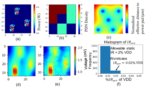
Figure 8: IREDGe static IR drop estimation on T11: (a) input power map, (b) input PDN density map, (c) effective distance to power pad map (d) ground truth IR drop map, (e) predicted IR drop map, and (f) histogram of $IR_{err}$ showing a worstcase error of 0.16mV.

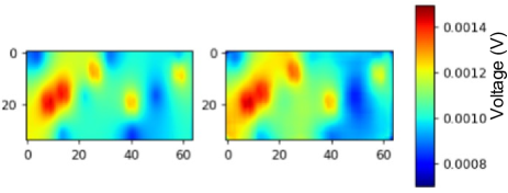
Figure 9: Size independent nature of IREDGe: Comparison between (a) Actual IR drop contours and (b) IREDGe-predicted contours for a power map (T16) with size 68$\times$32 using a model that was trained on images of size 34$\times$32.

A detailed view of T11 is shown in Fig. 8. It compares the IREDGe-generated IR drop contour plots against contour plot generated by [24]. The input power maps, PDN density maps, and effective distance to power pad maps are shown in Fig. 8(a), (b), and (c) respectively. Fig. 8(d) and (e) shows the comparison between ground truth and predicted value for the corresponding inputs. It is evident that the plots are similar; numerically, the histogram in Fig. 8(f) shows the %$IR_{err}$ where the worst %$IR_{err}$ is less than 0.02% of VDD.

Size-independence One of the primary advantages of using IREDGe for static IR estimation is that its fully-convolutional nature enables the use of input images of any size, and the size of the hotspot determines the model rather than the size of the chip. Since the trained model comprises only of the trained weights of the kernel, the same kernel can be used to predict the temperature contours of chip of any size as long as resolution of the represented image remains the same. We test static IREDGe on chips of a different size (T16 – T20), using a power distribution of size $68\times 32$ as input. Fig. 9(a) compares the actual IR drop of T16 (Fig. 9(a)) and the IREDGe-predicted (Fig. 9(b)) solution of T16 using a model which was trained on $34\times 32$ power maps. We summarize the results for the rest of the testcases in Table III.

Runtime analysis A summary of the runtime comparison of our ML-based EDGe network approach against the temperature and IR drop golden solvers is listed in Table IV. The runtimes are reported on a NVIDIA GeForce RTX 2080Ti GPU. With the millisecond inference times, and the transferable nature of our trained models, the one-time cost of training the EDGe networks is easily amortized over multiple uses within a design cycle, and over multiple designs.

TABLE IV: Runtime comparison between EDGe networks and golden thermal analysis and IR drop analysis tools

Analysis type	# Nodes	Design Area (mm2)	Icepak/ PDNSim (minutes)	ThermEDGe/ IREDGe (milli seconds)
Static thermal	2.0 million	64	30 mins	1.1 ms
Transient thermal	2.0 million	64	210 mins	10 ms
Static IR drop	5.2 million	0.16	310 mins	1.1 ms

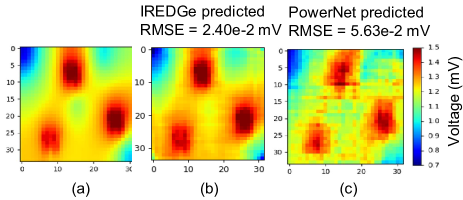
Figure 10: IR drop comparisons on T21: (a) ground truth, (b) from IREDGe, and (c) from our implementation of PowerNet.

IV-C IREDGe compared with PowerNet

We compare the performance of IREDGe against our implementation of PowerNet, based on its description in [8]. The layout is divided into tiles, and the CNN features are the 2-D power distributions (toggle rate-scaled switching and internal power, total power, and leakage power) within each tile and in a fixed window of surrounding tiles. The trained CNN is used to predict the IR drop on a tile-by-tile basis by sliding a window across all tiles on the chip. The work uses a tile size of 5$\mu$m$\times$5$\mu$m and takes into consideration a 31$\times$31 tiled neighborhood (window) power information as features. For a fair comparison, we train IREDGe under a fixed PDN density and fixed power pad locations that is used to train PowerNet. Qualitatively, IREDGe is superior on three aspects:
(1) Tile and window size selection: It is stated in [8] that when the size of the tile is increased from 1$\mu$m$\times$1$\mu$m to 5$\mu$m$\times$5$\mu$m and the size of the resulting window is increased to represent 31$\times$31 window of 25$\mu$m² tiles instead of 1$\mu$m² tiles, the accuracy of the PowerNet model improves. In general, this is the expected behavior with an IR analysis problem where the accuracy increases as more global information is available, until a certain radius after which the principle of locality holds [9]. IREDGe bypasses this tile-size selection problem entirely by providing the entire power map as input to IREDGe and allowing the network to learn the window size that is needed for accurate IR estimation.
(2) Run times: Unlike PowerNet, which trains and infers IR drop on a sliding tile-by-tile basis, IREDGe has faster training and inference. IREDGe requires a single inference, irrespective of the size of the chip while PowerNet performs an inference for every tile in the chip. For this setup and data, it takes 75 minutes to train and implementation of PowerNet, as against 30 minutes for IREDGe. For inference, PowerNet takes 3.2ms while IREDGe takes 1.1ms for a 34$\times$32 chip size. For a chip of $68\times 32$ IREDGe takes 1.3ms to generate IR drop contours while PowerNet takes 6.2ms.

(3) Model accuracy: Since PowerNet uses a CNN to predict IR drop on a region-by-region basis, where each region is 5$\mu$m by 5$\mu$m, the resulting IR drop image is pixelated, and the predicted region prediction value does not correlate well with the neighboring regions.

We compare IREDGe against our implementation of PowerNet on five different testcases T21–25. These testcases have the same power distribution in T11–15 except that all the five testscases have identical uniform PDNs, and identical power pad distributions, as required by PowerNet; IREDGe does not require this. Fig. 10 shows a comparison between the IR drop solutions from a golden solver (Fig. 10(a)), IREDGe (Fig. 10(b), and our implementation of PowerNet (Fig. 10(c)) for T21 (a representative testcase). On average, across T21–25 IREDGe has an average $IR_{err}$ of 0.028mV and a maximum $IR_{err}$ of 0.14mV as against 0.042mV and 0.17mV respectively for PowerNet.

V Conclusion

This paper addresses the compute-intensive tasks of thermal and IR analysis by proposing the use EDGe networks as apt ML-based solutions. Our EDGe-based solution not only improves runtimes but overcomes the window size-selection challenge (amount of neighborhood information required for accurate thermal and IR analysis), that is faced by other ML-based techniques, by allowing ML to learn the window size. We successfully evaluate EDGe networks for these applications by developing two ML software solutions (i) ThermEDGe and (ii) IREDGe for rapid on-chip (static and dynamic) thermal and (static) IR analysis respectively. In principle, our methodology is applicable to dynamic IR as well, but is not shown due to the unavailability of public-domain benchmarks.

References

- [1] Y. Zhan, S. V. Kumar, and S. S. Sapatnekar, “Thermally-aware design,” Found. Trends Electron. Des. Autom., vol. 2, no. 3, pp. 255–370, 2008.
- [2] Y. Zhong and M. D. F. Wong, “Fast algorithms for IR drop analysis in large power grid,” in Proc. ICCAD, 2005, pp. 351–357.
- [3] K. Zhang, A. Guliani et al., “Machine learning-based temperature prediction for runtime thermal management across system components,” IEEE Trans Parallel Distrib. Syst., vol. 29, no. 2, pp. 405–419, 2018.
- [4] D. Juan, Huapeng Zhou et al., “A learning-based autoregressive model for fast transient thermal analysis of chip-multiprocessors,” in Proc. ASP-DAC, 2012, pp. 597–602.
- [5] S. Sadiqbatcha, H. Zhao et al., “Hot spot identification and system parameterized thermal modeling for multi-core processors through infrared thermal imaging,” in Proc. DATE, 2019, pp. 48–53.
- [6] S.-Y. Lin, Y.-C. Fang et al., “IR drop prediction of ECO-revised circuits using machine learning,” in Proc. VLSI Test Symposium (VTS), 2018, pp. 1–6.
- [7] C. Ho and A. B. Kahng, “IncPIRD: Fast learning-based prediction of incremental IR drop,” in Proc. ICCAD, 2019, pp. 1–8.
- [8] Z. Xie, H. Ren et al., “PowerNet: Transferable dynamic IR drop estimation via maximum convolutional neural network,” in Proc. ASP-DAC, 2020, pp. 13–18.
- [9] E. Chiprout, “Fast flip-chip power grid analysis via locality and grid shells,” in Proc. ICCAD, 2004, pp. 485–488.
- [10] E. Shelhamer, J. Long, and T. Darrell, “Fully convolutional networks for semantic segmentation,” IEEE T. Pattern Anal. Mach. Intell., vol. 39, no. 4, pp. 640–651, 2017.
- [11] O. Ronneberger, P. Fischer, and T. Brox, “U-Net: Convolutional networks for biomedical image segmentation,” in Proc. Int. Conf. Med. Image Comput. Comput.-Assisted Intervention, 2015, pp. 234–241.
- [12] X. Mao, C. Shen, and Y.-B. Yang, “Image restoration using very deep convolutional encoder-decoder networks with symmetric skip connections,” in Proc. NeurIPS, 2016, pp. 2802–2810.
- [13] V. Badrinarayanan, A. Kendall, and R. Cipolla, “SegNet: A deep convolutional encoder-decoder architecture for image segmentation,” IEEE T. Pattern Anal. Mach. Intell., vol. 39, no. 12, pp. 2481–2495, 2017.
- [14] “Voltus IC Power Integrity Solution,” www.cadence.com/en_US/home/tools/digital-design-and-signoff/silicon-signoff/voltus-ic-power-integrity-solution.html.
- [15] J. Singh and S. S. Sapatnekar, “Partition-based algorithm for power grid design using locality,” IEEE T. Comput. Aid D., vol. 25, no. 4, pp. 664–677, 2006.
- [16] V. A. Chhabria, A. B. Kahng et al., “Template-based PDN synthesis in floorplan and placement using classifier and CNN techniques,” in Proc. ASP-DAC, 2020, pp. 44–49.
- [17] B. W. Amick, C. R. Gauthier, and D. Liu, “Macro-modeling concepts for the chip electrical interface,” in Proc. DAC, 2002, p. 391–394.
- [18] F. Yazdani, “Foundations of heterogeneous integration: An industry-based, 2.5d/3d pathfinding and co-design approach.” Boston, MA: Springer, 2018.
- [19] I. Sutskever, O. Vinyals, and Q. V. Le, “Sequence to sequence learning with neural networks,” in Proc. NeurIPS, 2014, pp. 3104–3112.
- [20] V. Dumoulin and F. Visin, “A guide to convolution arithmetic for deep learning,” arXiv:1603.07285v2, Mar. 2016.
- [21] W. Luo, Y. Li et al., “Understanding the effective receptive field in deep convolutional neural networks,” in Proc. NeurIPS, 2016, pp. 4905–4913.
- [22] X. Shi, Z. Chen et al., “Convolutional LSTM network: A machine learning approach for precipitation nowcasting,” in Proc. NeurIPS, 2015, pp. 802–810.
- [23] “Ansys-Icepak,” www.ansys.com/products/electronics/ansys-icepak.
- [24] “PDNSim,” github.com/The-OpenROAD-Project/PDNSim.
- [25] S. R. Nassif, “Power grid analysis benchmarks,” in Proc. ASP-DAC. IEEE Computer Society Press, 2008, p. 376–381.
- [26] D. Kingma and J. Ba, “ADAM: A method for stochastic optimization,” in Proc. ICLR, 2014.