A design framework for actively crosslinked filament networks

Abstract

Living matter moves, deforms, and organizes itself. In cells this is made possible by networks of polymer filaments and crosslinking molecules that connect filaments to each other and that act as motors to do mechanical work on the network. For the case of highly cross-linked filament networks, we discuss how the material properties of assemblies emerge from the forces exerted by microscopic agents. First, we introduce a phenomenological model that characterizes the forces that crosslink populations exert between filaments. Second, we derive a theory that predicts the material properties of highly crosslinked filament networks, given the crosslinks present. Third, we discuss which properties of crosslinks set the material properties and behavior of highly crosslinked cytoskeletal networks. The work presented here, will enable the better understanding of cytoskeletal mechanics and its molecular underpinnings. This theory is also a first step towards a theory of how molecular perturbations impact cytoskeletal organization, and provides a framework for designing cytoskeletal networks with desirable properties in the lab.

I Introduction

Materials made from constituents that use energy to move are called active. These inherently out of equilibrium systems have attractive physical properties: active materials can spontaneously form patterns bois2011pattern , collectively move voituriez2005spontaneous ; furthauer2012taylor ; wioland2013confinement , self-organize into structures salbreux2009hydrodynamics ; brugues2014physical , and do work marchetti2013hydrodynamics . Biology, through evolution, has found ways to exploit this potential. The cytoskeleton, an active material made from biopolymer filaments and molecular scale motors, drives cellular functions with remarkable spatial and temporal coordination alberts_2002_book ; howard2001mechanics . The ability of cells to move, divide, and deform relies on this robust, dynamic and adaptive material. To understand the molecular underpinnings of cellular mechanics and design similarly useful active matter systems in the lab, a theory that predicts their behavior from the interactions between their constituents is needed. The aim of this paper, is to address this challenge for highly crosslinked systems made from rigid rod-like filaments and molecular scale motors.

The large-scale physics of active materials can be described by phenomenological theories, which are derived from symmetry considerations and conservation laws, without making assumptions on the detailed molecular scale interactions that give rise to the materials properties kruse2004asters ; furthauer2012active ; julicher2018hydrodynamic . This has allowed exploring the exotic properties of active materials, and the quantitative description of subcellular structures, such as the spindle brugues2014physical ; oriola2020active (the structure that segregates chromosomes during cell division) and the cell cortexmayer2010anisotropies ; salbreux2012actin ; naganathan2014active ; naganathan2018morphogenetic (the structure that provides eukaryotic cells with the ability to control their shape), even though the microscale processes at work often remain opaque. In contrast, understanding how molecular perturbations affect cellular scale structures requires theories that explain how material properties depend on the underlying molecular behaviors. Designing active materials with desirable properties in the lab will also require the ability to predict how emergent properties of materials result from their constituents foster2019cytoskeletal . Until now, the attempts to bridge this gap have relied heavily on computational methods belmonte2017theory ; foster2017connecting ; gao2015multiscalepolar , or were restricted to sparsely crosslinked systems liverpool2003instabilities ; liverpool2005bridging ; liverpool2008hydrodynamics ; aranson2005pattern ; saintillan2008instabilitiesPRL , one dimensional systems kruse2000actively ; kruse2003self , or systems with permanent crosslinks broedersz2014modeling . Our interest here are cytoskeletal networks, which are in general highly crosslinked by tens to hundreds of transient crosslinks linking each filament into the network. In this regime, the forces generated by different crosslinks in the network balance against each other, and not against friction with the surrounding medium, as they would in a sparsely crosslinked regime furthauer2019self .

We derive how the large scale properties of an actively crosslinked network of cytoskeletal filaments depend on the micro-scale interactions between its components. This theory generalizes our earlier work on one specific type of motor-filament mixture, XCTK2 and microtubules furthauer2019self ; striebel2020mechanistic , by introducing a generic phenomenological model to describe the forces that crosslink populations exert between filaments.

The structure of this paper is as follows. In section II, we discuss the force and torque balance for systems of interacting particles, and specialize to the case of interacting rod-like filaments. This will allow us to introduce key concepts of the continuum description, such as the network stress tensor. Next, in section III, we present a phenomenological model for crosslink interactions between filaments, that can describe the properties of many different types of crosslinks in terms of just a few parameters, which we call crosslink moments. In section IV, we derive the continuum theory for highly crosslinked active networks and obtain the equations of motion for these systems. Finally, in section V we give an overview of the main predictions of our theory and discuss the consequences of specific micro-scale properties for the mechanical properties of the consequent active material. We summarize and contextualize our findings in the discussion section VI.

II Force and torque balance in systems of interacting rod-like particles

We start by discussing the generic framework of our description. In this section we give equations for particle, momentum and angular momentum conservation and introduce the stress tensor, for generic systems of particles with short ranged interactions. We then specialize to the case of interacting rod-like filaments, which form the networks that we study here.

II.1 Particle Number Continuity

Consider a material that consists of a large number $N$ of particles, that are characterized by their center of mass positions $\mathbf{x}_{i}$ and their orientations $\mathbf{p}_{i}$, where $|\mathbf{p}_{i}|=1$ is an unit vector and $i$ is the particle index. We define the particle number density

$$\psi(\mathbf{x},\mathbf{p})=\sum_{i}\delta(\mathbf{x}-\mathbf{x}_{i})\delta(\mathbf{p}-\mathbf{p}_{i}).$$ (1)

Here and in the following $\delta(\mathbf{x}-\mathbf{x}_{i})$ has dimensions of inverse volume, while $\delta(\mathbf{p}-\mathbf{p}_{i})$ is dimensionless. Ultimately, our goal is to predict how $\psi$ changes over time. This is given by the Smoluchowski equation

$$\partial_{t}\psi(\mathbf{x},\mathbf{p})=-\nabla\cdot\left(\dot{\mathbf{x}}\psi\right)-\partial_{\mathbf{p}}\cdot\left(\dot{\mathbf{p}}\psi\right),$$ (2)

where

$$\dot{\mathbf{x}}\psi=\sum_{i}\dot{\mathbf{x}}_{i}\delta(\mathbf{x}-\mathbf{x}_{i})\delta(\mathbf{p}-\mathbf{p}_{i})$$ (3)

and

$$\dot{\mathbf{p}}\psi=\sum_{i}\dot{\mathbf{p}}_{i}\delta(\mathbf{x}-\mathbf{x}_{i})\delta(\mathbf{p}-\mathbf{p}_{i})$$ (4)

define $\dot{\mathbf{x}}$ and $\dot{\mathbf{p}}$, the fluxes of particle position and orientation. The aim of this paper is to derive $\dot{\mathbf{x}}$ and $\dot{\mathbf{p}}$, from the forces and torques that act on and between particles.

II.2 Force Balance

Each particle in the active network obeys Newton’s laws of motion. That is

$$\dot{\mathbf{g}}_{i}=\sum_{j}\mathbf{F}_{ij}\mathbf{+}\mathbf{F}_{i}^{\mathrm{(drag)}},$$ (5)

where $\mathbf{g}_{i}$ is the particle momentum, and $\mathbf{F}_{ij}$ is the force that particle $j$ exerts on particle $i$. Moreover, $\mathbf{F}_{i}^{\mathrm{(drag)}}$ is the drag force between the particle $i$ and the fluid in which it is immersed. Momentum conservation implies $\mathbf{F}_{ij}=-\mathbf{F}_{ji}$. We are interested in systems where the direct particle-particle interactions are short ranged. This means that $\mathbf{F}_{ij}\neq 0$ only if $|\mathbf{x}_{i}-\mathbf{x}_{j}|<d$, where $d$ is an interaction length that is small (relative to system size).

The momentum density is defined by

$$\mathbf{g}=\sum_{i}\delta(\mathbf{x}-\mathbf{x}_{i})\mathbf{g}_{i}$$ (6)

which, using Eq. (5), obeys

$$\partial_{t}\mathbf{g} + \nabla\cdot\sum_{i}\delta(\mathbf{x}-\mathbf{x}_{i})\mathbf{v}_{i}\mathbf{g}_{i}=\sum_{i,j}\delta(\mathbf{x}-\mathbf{x}_{i})\mathbf{F}_{ij}+\sum_{i}\delta(\mathbf{x}-\mathbf{x}_{i})\mathbf{F}^{\mathrm{(drag)}}_{i},$$

where $\mathbf{v}_{i}=\dot{\mathbf{x}}_{i}$ is the velocity of the $i$-th particle. The terms on the left hand side of Eq. (LABEL:eq:Fb_continuum) are inertial, and in the overdamped limit, relevant to the systems studied here, they are vanishingly small. Interactions between particles are described by the first term on the right hand side of Eq. (LABEL:eq:Fb_continuum) and generate a momentum density flux $\mathbf{\Sigma}$ (the stress tensor) through the material. To wit, using that $d$ is small, so that particle-particle interactions are short-ranged, gives

$$\sum_{i,j}\delta(\mathbf{x}-\mathbf{x}_{i})\mathbf{F}_{ij}=\frac{1}{2}\sum_{i,j}\left(\delta(\mathbf{x}-\mathbf{x}_{i})-\delta(\mathbf{x}-\mathbf{x}_{j})\right)\mathbf{F}_{ij}$$ (8)

$$= -\nabla\cdot\sum_{i,j}\delta\left(\mathbf{x}-\mathbf{x}_{i}\right)\frac{\mathbf{x}_{i}-\mathbf{x}_{j}}{2}\mathbf{F}_{ij}+\mathcal{O}(d^{3})$$

$$= \nabla\cdot\mathbf{\Sigma}.$$

where

$$\mathbf{\Sigma}=-\sum_{i,j}\delta\left(\mathbf{x}-\mathbf{x}_{i}\right)\frac{\mathbf{x}_{i}-\mathbf{x}_{j}}{2}\mathbf{F}_{ij}+\mathcal{O}(d^{3}).$$ (9)

Note that Eq. (9) does not necessarily produce a symmetric stress tensor. Force couples for which $\mathbf{F}_{ij}$ and $\mathbf{x}_{i}-\mathbf{x}_{j}$ are not parallel generate antisymmetric stress contributions, since these couples are not torque free. We discuss how to reconcile this with angular momentum conservation in Appendix C. The drag force density is

$$\mathbf{f}=\sum_{i}\delta(\mathbf{x}-\mathbf{x}_{i})\mathbf{F}_{i}^{\mathrm{(drag)}},$$ (10)

and after dropping inertial terms, the force balance reads

$$\nabla\cdot\mathbf{\Sigma}+\mathbf{f}=\mathbf{0},$$ (11)

and the total force on particle $i$ obeys

$$\sum_{j}\mathbf{F}_{ij}+\mathbf{F}_{i}^{\mathrm{(drag)}}=\mathbf{0}.$$ (12)

This completes the discussion of the force balance of the system. We next discuss angular momentum conservation.

II.3 Torque Balance

The total angular momentum of particle $i$,

$$\mathbf{\ell}^{\mathrm{(tot)}}_{i}=\mathbf{\ell}_{i}+\mathbf{x}_{i}\times\mathbf{g}_{i},$$ (13)

is conserved, where $\mathbf{\ell}_{i}$ is its spin angular momentum and its $\mathbf{x}_{i}\times\mathbf{g}_{i}$ its orbital angular momentum. Newton’s laws imply that

$$\dot{\mathbf{\ell}}_{i}=\sum_{j}\mathbf{T}_{ij}+\mathbf{T}_{i}^{\mathrm{(drag)}},$$ (14)

where $\mathbf{T}_{ij}$ is the torque exerted by particle $j$ on particle $i$, in the frame of reference moving with particle $i$,nd $\mathbf{T}_{i}^{\mathrm{(drag)}}$ is the torque from interaction with the medium, in the same frame of reference. Importantly, since the total angular momentum is a conserved quantity, the total torque transmitted between particles $\mathbf{T}_{ij}+\mathbf{x}_{i}\times\mathbf{F}_{ij}=-\mathbf{T}_{ji}-\mathbf{x}_{j}\times\mathbf{F}_{ji}$ is odd upon exchange of the particle indices $i$ and $j$. Taking a time derivative of Eq. (13) and using Eq. (5) leads to the torque balance equation for particle $i$

$$\sum_{j}\left(\mathbf{T}_{ij}+\mathbf{x}_{i}\times\mathbf{F}_{ij}\right)+\mathbf{T}_{i}^{\mathrm{(drag)}}+\mathbf{x}_{i}\times\mathbf{F}_{i}^{\mathrm{(drag)}}=\mathbf{0},$$ (15)

and thus

$$\sum_{j}\mathbf{T}_{ij}+\mathbf{T}_{i}^{\mathrm{(drag)}}=\mathbf{0},$$ (16)

where we ignored the inertial term $\mathbf{v}_{i}\times\mathbf{g}_{i}$ and used Eq. (12). The angular momentum fluxes associated with spin, orbital and total angular momentum are discussed in Appendix C for completeness.

II.4 The special case of rod-like filaments

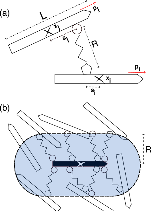
Figure 1: a/ Interaction between two cytoskeletal filament $i$ and $j$ via a molecular motor. Filaments are characterized by their positions $\mathbf{x}_{i},\mathbf{x}_{j}$, their orientations $\mathbf{p}_{i},\mathbf{p}_{j}$, and connect by a motor between arc-length position $s_{i},s_{j}$. A motor consist of two heads that can be different (circle, pentagon) and are connected by a linker (black zig-zag) of lengt $R$ b/ The total force on filament $i$ is given by the sum of the forces exerted by all $a$ (circle) and $b$ (pentagon) heads, which connect the filament into the network. The shaded area shows all geometrically accessible positions that can be crosslinked to the central (black) filament.

We now specialize to rod-like particles, such as the microtubules and actin filaments that make up the cytoskeleton. In particular, we calculate the objects $\mathbf{F}_{ij}$, $\mathbf{T}_{ij}$, and $\mathbf{\Sigma}$ from prescribed interaction forces and torques along rod-like particles.

II.4.1 Forces

Again, filament $i$ is described by it center of mass $\mathbf{x}_{i}$ and orientation vector $\mathbf{p_{i}}$. All filaments are taken as having the same length $L$, and position along filament $i$ is given by $\mathbf{x}_{i}+s_{i}\mathbf{p}_{i}$, where $s_{i}\in[-L/2,L/2]$ is the signed arclength. We consider the vectorial momentum flux from arclength position $s_{i}$ on filament $i$ to arclength position $s_{j}$ on filament $j$

$$\mathbf{f}_{ij}=\mathbf{f}_{ij}\left(s_{i},s_{j}\right).$$ (17)

where $\mathbf{f}_{ij}=-\mathbf{f}_{ji}$ and having dimensions of force over area, i.e. a stress. Here we focus on forces generated by crosslinks; see Fig. 1 (a). The total force between two particles is

$$\mathbf{F}_{ij} = \left\lfloor\delta(\mathbf{x}-\mathbf{x}_{j}-s_{j}\mathbf{p}_{j})\mathbf{f}_{ij}\right\rceil^{ij}_{\Omega(\mathbf{x}_{i}+s_{i}\mathbf{p}_{i})},$$

where the brackets $\lfloor\cdots\rceil^{ij}_{\Omega(\mathbf{x}_{i})}$ denote the operation

$$\lfloor\phi\rceil_{\Omega(\mathbf{x}_{i})}^{ij}=\int\limits_{-\frac{L}{2}}^{\frac{L}{2}}ds_{i}\int\limits_{-\frac{L}{2}}^{\frac{L}{2}}ds_{j}\int\limits_{\Omega(\mathbf{x}_{i})}d\mathbf{x}^{3}\phi,$$ (19)

where $\phi$ is a dummy argument and $\Omega$ is a sphere whose radius is the size of a cross-linker (i.e., $d$, the interaction distance). With the definition Eq. (19), the operation $\lfloor\cdots\rceil^{ij}_{\Omega(\mathbf{x}_{i}+s_{i}\mathbf{p}_{i})}$ integrates its argument over all geometrically possible crosslink interactions, between filaments $i$ and $j$; see Fig. 1 (b). By Taylor expanding and keeping terms up to second order in the filament arc length $(s_{i},s_{j})$, we find

$$\mathbf{F}_{i}^{\mathrm{(tot)}}=\sum_{j}\left\lfloor\left\{\begin{array}[]{c}1\\ +(s_{i}\mathbf{p}_{i}-s_{j}\mathbf{p}_{j})\cdot\nabla\\ +\frac{1}{2}(s_{i}^{2}\mathbf{p}_{i}\mathbf{p}_{i}+s_{j}^{2}\mathbf{p}_{j}\mathbf{p}_{j}):\nabla\nabla\end{array}\right\}\delta(\mathbf{x}-\mathbf{x}_{j})\mathbf{f}_{ij}\right\rceil_{\Omega(\mathbf{x}_{i})}^{ij}+\mathbf{F}_{i}^{\mathrm{(drag)}}$$ (23)

(24)

and the network stress

$$\mathbf{\Sigma}=-\frac{1}{2}\sum_{i,j}\left\lfloor\begin{array}[]{c}\delta(\mathbf{x}-\mathbf{x}_{i})\delta(\mathbf{x}^{\prime}-\mathbf{x}_{j})\\ \left(\mathbf{x}_{i}-\mathbf{x}_{j}+s_{i}\mathbf{p}_{i}-s_{j}\mathbf{p}_{j}\right)\mathbf{f}_{ij}\end{array}\right\rceil_{\Omega(\mathbf{x}_{i})}^{ij}$$ (27)

where we used that $\mathbf{f}_{ij}=-\mathbf{f}_{ji}$.

II.4.2 Torques

Similarly, the angular momentum flux that crosslinkers exert between filaments can be written as

$$\mathbf{t}_{ij}=\bar{\mathbf{t}}_{ij}\left(s_{i},s_{j}\right)+s_{i}\mathbf{p}_{i}\times\mathbf{f}_{ij},$$ (28)

which dimensionally is a torque per unit area. Thus

$$\mathbf{T}_{ij}=\lfloor\delta(\mathbf{x}-\mathbf{x}_{j}-s_{j}\mathbf{p}_{j})\mathbf{t}_{ij}\rceil_{\Omega(\mathbf{x}_{i}+s_{i}\mathbf{p}_{i})}$$ (29)

which leads to

$$\mathbf{T}_{i}^{\mathrm{(tot)}}=\mathbf{T}_{i}^{\mathrm{(drag)}}+\sum_{j}\left\lfloor\begin{array}[]{c}\delta(\mathbf{x}-\mathbf{x}_{j})\left(\bar{\mathbf{t}}_{ij}+s_{i}\mathbf{p}_{i}\times\mathbf{f}_{ij}\right)\\ +(s_{i}\mathbf{p}_{i}-s_{j}\mathbf{p}_{j})\cdot\nabla\delta(\mathbf{x}-\mathbf{x}_{j})\left(\bar{\mathbf{t}}_{ij}+s_{i}\mathbf{p}_{i}\times\mathbf{f}_{ij}\right)\\ +\frac{1}{2}(s^{2}_{i}\mathbf{p}_{i}\mathbf{p}_{i}+s^{2}_{j}\mathbf{p}_{j}\mathbf{p}_{j}):\nabla\nabla\delta(\mathbf{x}-\mathbf{x}_{j})\bar{\mathbf{t}}_{ij}\end{array}\right\rceil_{\Omega(\mathbf{x}_{i})}^{ij}$$ (33)

(34)

In the following we will consider crosslinks for which $\bar{\mathbf{t}}_{ij}=0$, for simplicity.

III Filament-Filament interactions by crosslinks and collisions

We next discuss how filaments in highly crosslinked networks exchange linear and angular momentum. Two types of interactions are important here: interactions mediated by crosslinking molecules, which can be simple static linkers or active molecular motors, and steric interactions. We start by discussing the former.

III.1 Crosslinking interactions

To describe crosslinking interactions, we propose a phenomenological model for the stress $\mathbf{f}_{ij}$ that crosslinkers exert between the attachment positions $s_{i}$ and $s_{j}$ on filaments $i$ and $j$.

$$\mathbf{f}_{ij} = K(s_{i},s_{j},t)\left(\mathbf{x}_{i}+s_{i}\mathbf{p}_{i}-\mathbf{x}_{j}-s_{j}\mathbf{p}_{j}\right)$$ (35)

$$+ \gamma(s_{i},s_{j},t)\left(\mathbf{v}_{i}+s_{i}\dot{\mathbf{p}}_{i}-\mathbf{v}_{j}-s_{j}\dot{\mathbf{p}}_{j}\right)$$

$$+ \left[\sigma(s_{i},s_{j},t)\mathbf{p}_{i}-\sigma(s_{j},s_{i},t)\mathbf{p}_{j}\right],$$

The first term in this model, with coefficient $K$, is proportional to the displacement between between the attachment points, $\mathbf{x}_{i}+s_{i}\mathbf{p}_{i}-\mathbf{x}_{j}-s_{j}\mathbf{p}_{j}$, and captures the effects of crosslink elasticity and motor slow-down under force. The second term, with coefficient $\gamma$, is proportional to $\mathbf{v}_{i}+s_{i}\dot{\mathbf{p}}_{i}-\mathbf{v}_{j}-s_{j}\dot{\mathbf{p}}_{j}$, and captures friction-like effects arising from velocity differences between the attachment points. The last terms are motor forces that act along filament orientations $\mathbf{p}_{i}$ and $\mathbf{p}_{j}$, with their coefficients $\sigma$ having dimensions of stress. Additional forces proportional to the relative rotation rate between filaments, $\dot{\mathbf{p}}_{i}-\dot{\mathbf{p}}_{j}$, are allowed by symmetry, but are neglected here for simplicity.

In general, the coefficients $K$, $\gamma$, and $\sigma$ are tensors that depend on time, the relative orientations between microtubule $i$ and $j$ and the attachment positions $s_{i},s_{j}$ on both filaments. In this work, we take them to be scalar and independent of the relative orientation, for simplicity. Generalizing the calculations that follow to include the dependences of $K,\gamma$ and $\sigma$ on $\mathbf{p}_{i}$ and $\mathbf{p}_{j}$ is straightforward but laborious and will be discussed in a subsequent publication. We emphasize that Eq. (35) is a statement about the expected average effect of crosslinks in a dense local environment and is not a description of individual crosslinking events.

Inserting Eq.(35) into Eqs. (24, 27, 34) we find that the stresses and forces collectively generated by crosslinks depend on $s_{ij}$-moments of the form

$$X_{nm}(\mathbf{x})=\lfloor X(s_{i},s_{j})s_{i}^{n}s_{j}^{m}\rceil_{\Omega(\mathbf{x})}^{ij},$$ (36)

where $X=K$, $\gamma$, or $\sigma$. We refer to these as crosslink moments. In principle, given Eqs.(24, 27, 35) only the moments $X_{00},X_{01},X_{10},X_{11},X_{20},X_{02},X_{21},$ and $X_{12}$, contribute to the stresses and forces in the filament network. We further note that $X_{11}$, $X_{21}$ and $X_{12}$ are $\mathcal{O}(L^{4})$, and can thus be neglected without breaking asymptotic consistency. Moreover, $X_{20}$ and $X_{02}$ can be expressed in terms of lower order moments since $X_{20}=X_{02}+\mathcal{O}(L^{4})=(L^{2}/12)X_{00}+\mathcal{O}(L^{4})$.

Finally, by construction $K(s_{i},s_{j})=K(s_{j},s_{i})$ and $\gamma(s_{i},s_{j})=\gamma(s_{j},s_{i})$, and thus $\gamma_{01}=\gamma_{10}\equiv\gamma_{1}$ and $K_{01}=K_{10}\equiv K_{1}$. To further simplify our notation, we introduce $X_{0}=X_{00}$. Explicit expressions for the seven crosslinking moments that contribute to the continuum theory are given in the Appendix B. In summary, in the long wave length limit all forces and stresses in the network can be expressed in terms of just a few moments, $K_{0},K_{1},\gamma_{0},\gamma_{1},\sigma_{0},\sigma_{01},\sigma_{10}$. How different crosslinker behavior set these moments will be discussed in SectionV.

III.2 Sterically mediated interactions

In addition to crosslinker mediated forces and torques, steric interactions between filaments generate momentum and angular momentum transfer in the system. We model steric interactions by a free energy $E=\int_{\mathcal{V}}e(\mathbf{p}_{i},\cdots,\mathbf{x}_{i},\cdots)d^{3}x$ which depends on all particle positions and orientations. The steric force is

$$\bar{\mathbf{F}}_{i}=-\frac{\delta E}{\delta\mathbf{x}_{i}},$$ (37)

and the torque acting on it is

$$\bar{\mathbf{T}}_{i}=-\frac{\delta E}{\delta\mathbf{p}_{i}}.$$ (38)

This approach is commonly used throughout soft matter physics martin1972unified ; chaikin2000principles . Common choices for the free energy density $e$ are the ones proposed by Maier and Saupe doi1988theory , or Landau and DeGennes de1993physics .

IV Continuum Theory for highly crosslinked active networks

In the previous sections we derived a generic expression for the stresses and forces acting in a network of filaments interacting through local forces and torques, and proposed a phenomenological model for crosslink-driven interactions between filaments. We now combine these two and obtain expressions for the stresses, force, and torques acting in a highly crosslinked filament network, and from there derive equations of motion for the material. We start by introducing the coarse-grain fields in terms of which our theory is phrased.

IV.1 Continuous Fields

The coarse grained fields of relevance are the number density,

$$\rho=\sum_{i}\delta(\mathbf{x}-\mathbf{x}_{i}),$$ (39)

the velocity $\mathbf{v}=\left<\mathbf{v}_{i}\right>$, the polarity $\mathbf{P}=\left<\mathbf{p}_{i}\right>$, the nematic-order tensor $\mathcal{Q}=\left<\mathbf{p}_{i}\mathbf{p}_{i}\right>$, and the third and fourth order tensors $\mathcal{T}=\left<\mathbf{p}_{i}\mathbf{p}_{i}\mathbf{p}_{i}\right>$, and $\mathcal{S}=\left<\mathbf{p}_{i}\mathbf{p}_{i}\mathbf{p}_{i}\mathbf{p}_{i}\right>$. Here the brackets $\left<\cdot\right>$ signify the averaging operation

$$\rho\left<\phi_{i}\right>=\sum_{i}\delta(\mathbf{x}-\mathbf{x}_{i})\phi_{i},$$ (40)

where $\phi_{i}$ is a dummy variable. Furthermore, we define the tensors $\mathbf{j}=\left<\mathbf{p}_{i}\left(\mathbf{v}_{i}-\mathbf{v}\right)\right>$, $\mathcal{J}=\left<\mathbf{p}_{i}\mathbf{p}_{i}\left(\mathbf{v}_{i}-\mathbf{v}\right)\right>$, $\mathcal{H}=\left<\mathbf{p}_{i}\dot{\mathbf{p}}_{i}\right>$, and the rotation rate $\mathbf{\omega}=\left<\dot{\mathbf{p}}_{i}\right>$.

IV.2 Stresses

The presence of crosslinkers generates stresses in the material which, through Eq. (27), depends on the crosslinking force density Eq. (35). Following the nomenclature from Eq. (35), we write the material stress as

$$\mathbf{\Sigma}=\mathbf{\Sigma}^{(K)}+\mathbf{\Sigma}^{(\gamma)}+\mathbf{\Sigma}^{(V)}+\mathbf{\bar{\Sigma}},$$ (41)

where

$$\mathbf{\Sigma}^{(K)}=-\rho^{2}K_{0}\left(\alpha\mathcal{I}+\frac{L^{2}}{12}\mathcal{Q}\right),$$ (42)

is the stress due to the crosslink elasticity,

$$\mathbf{\Sigma}^{(\gamma)}=-\rho^{2}\left(\eta\nabla\mathbf{v}+\gamma_{1}\mathbf{j}+\gamma_{0}\frac{L^{2}}{12}\mathcal{H}\right),$$ (43)

is the viscous like stress generated by crosslinkers, and

$$\mathbf{\Sigma}^{(V)}=-\rho^{2}\left(\alpha\sigma_{0}\nabla\mathbf{P}+\sigma_{10}\mathcal{Q}-\sigma_{01}\mathbf{P}\mathbf{P}\right)$$ (44)

is the stress generated by motor stepping. Here, we defined the network viscosity $\eta=\alpha\gamma_{0}$ and $\alpha=\frac{3R^{2}}{10}$.

Finally, the steric (or Ericksen) stress obeys the Gibbs Duhem Relation

$$\nabla\cdot\bar{\mathbf{\Sigma}}=\rho\nabla\mu+(\nabla\mathcal{E}):\mathcal{Q}.$$ (45)

where $\mu=-\frac{\delta e}{\delta\rho}$ is the chemical potential, and $\mathcal{E}=-\frac{\delta e}{\delta\mathcal{Q}}$ is the steric distortion field. An explicit definition of $\bar{\mathbf{\Sigma}}$ and the derivation of the Gibbs Duhem relation are given in Appendix (D). Note that for simplicity, we chose that the steric free energy density $e$ depends only on nematic order and not on polarity.

IV.3 Forces

We now calculate the forces acting on filament $i$. The total force $\mathbf{F}_{i}$ on filament $i$ is given by

$$\mathbf{F}_{i}=\mathbf{F}_{i}^{(K)}+\mathbf{F}_{i}^{(\gamma)}+\mathbf{F}_{i}^{(V)}+\bar{\mathbf{F}}_{i}+\mathbf{F}_{i}^{\mathrm{(drag)}},$$ (46)

where

$$\mathbf{F}^{(K)}_{i} = (\nabla\rho)\cdot\frac{L^{2}}{12}K_{0}(\mathbf{p}_{i}\mathbf{p}_{i}-\mathcal{Q})-\frac{1}{\rho}\nabla\cdot\mathbf{\Sigma}^{(K)},$$ (47)

is the elasticity driven force

$$\mathbf{F}_{i}^{(\gamma)} = \gamma_{0}\rho(\mathbf{v}_{i}-\mathbf{v})+\gamma_{1}\rho(\dot{\mathbf{p}}_{i}-\mathbf{\omega})$$ (48)

$$+ \gamma_{1}\left(\nabla\rho\right)\cdot\left[\mathbf{p}_{i}\left(\mathbf{v}_{i}-\mathbf{v}\right)-\mathbf{j}-\mathbf{P}\left(\mathbf{v}_{i}-\mathbf{v}\right)\right]$$

$$+ \frac{L^{2}}{12}\gamma_{0}\left(\nabla\rho\right)\cdot\left[\mathbf{p}_{i}\dot{\mathbf{p}}_{i}-\mathcal{H}\right]$$

$$+ \frac{L^{2}}{12}\gamma_{0}\left(\nabla\nabla\rho\right):\left[\mathbf{p}_{i}{\mathbf{p}}_{i}\left(\mathbf{v}_{i}-\mathbf{v}\right)-\mathcal{J}+\mathcal{Q}\left(\mathbf{v}_{i}-\mathbf{v}\right)\right]$$

$$- \frac{1}{\rho}\nabla\cdot\mathbf{\Sigma}^{(\gamma)}.$$

is the viscous like force, and

$$\mathbf{F}_{i}^{(V)} = \rho\sigma_{0}(\mathbf{p}_{i}-\mathbf{P})$$ (49)

$$+ (\nabla\rho)\cdot\left[\sigma_{10}\left(\mathbf{p}_{i}\mathbf{p}_{i}-\mathcal{Q}\right)-\sigma_{01}\left(\mathbf{p}_{i}\mathbf{P}+\mathbf{P}\mathbf{p}_{i}-2\mathbf{P}\mathbf{P}\right)\right]$$

$$+ \frac{L^{2}}{12}\sigma_{0}(\nabla\nabla\rho):\left[\mathbf{p}_{i}\mathbf{p}_{i}\mathbf{p}_{i}+\mathcal{Q}\mathbf{p}_{i}-\mathbf{p}_{i}\mathbf{p}_{i}\mathbf{P}-\mathcal{T}\right]$$

$$- \frac{1}{\rho}\nabla\cdot\mathbf{\Sigma}^{(V)}.$$

is the motor force. Finally,

$$\bar{\mathbf{F}}_{i}=-\frac{\nabla\mathcal{E}}{\rho}:(\mathbf{p}_{i}\mathbf{p}_{i}-\mathcal{Q})-\frac{1}{\rho}\nabla\cdot\bar{\mathbf{\Sigma}},$$ (50)

is the steric force on filament $i$, where we again chose $e$ to only depend on nematic order and not on polarity.

IV.4 Crosslinker induced Torque

We next calculate the torques acting on filament $i$. The total torque acting on filament $i$ is

$$\mathbf{T}_{i}=\mathbf{T}_{i}^{(\gamma)}+\mathbf{T}_{i}^{(V)}+\bar{\mathbf{T}}_{i}+\mathbf{T}_{i}^{(\mathrm{drag})}$$ (51)

Note, that crosslinker elasticity does not contribute. Here

$$\mathbf{T}_{i}^{(\gamma)} = \gamma_{1}\rho\mathbf{p}_{i}\times\left(\mathbf{v}_{i}-\mathbf{v}\right)+\frac{L^{2}}{12}\gamma_{0}\rho\mathbf{p}_{i}\times\dot{\mathbf{p}}_{i}$$ (52)

$$+ \frac{L^{2}}{12}\gamma_{0}\mathbf{p}_{i}\times\left(\mathbf{p}_{i}\cdot\nabla\rho\right)\left(\mathbf{v}_{i}-\mathbf{v}\right)$$

$$- \frac{L^{2}}{12}\gamma_{0}\rho\mathbf{p}_{i}\times(\mathbf{p}_{i}\cdot\nabla\mathbf{v})$$

and

$$\mathbf{T}^{(V)}_{i} = -\rho\mathbf{p}_{i}\times\left(\sigma_{01}\mathbf{P}+\frac{L^{2}}{12}\sigma_{0}\mathbf{p}_{i}\cdot\nabla\mathbf{P}\right)-\frac{L^{2}}{12}\sigma_{0}\mathbf{p}_{i}\times(\mathbf{p}_{i}\cdot\nabla\rho)\mathbf{P}$$ (53)

are the viscous and motor torques, respectively. Steric interactions contribute to the torque

$$\bar{\mathbf{T}}_{i}=\mathbf{p}_{i}\times\frac{\mathcal{E}}{\rho}\cdot\mathbf{p}_{i}.$$ (54)

IV.5 Equations of Motion

To find equations of motion for the highly crosslinked network, we use Eqs. (46, 47, 48, 49), and obtain

$$\mathbf{v}_{i}-\mathbf{v} = -\frac{\sigma_{0}}{\gamma_{0}}(\mathbf{p}_{i}-\mathbf{P})-\frac{1}{\rho\gamma_{0}}\left(\mathbf{F}^{\mathrm{(drag)}}_{i}-f/\rho\right)+\mathcal{O}\left(L^{2}\right),$$ (55)

which will be a useful low-order approximation to $\mathbf{v}_{i}-\mathbf{v}$. Note too that we have dropped steric forces, since $\nabla\mathcal{E}/\rho$ scales with the inverse of the system size, which is much larger than $L$. Using Eq. (55) in Eq. (51) we find the equation of motion for filament rotations,

$$\dot{\mathbf{p}}_{i} = \left(\mathcal{I}-\mathbf{p}_{i}\mathbf{p}_{i}\right)\cdot\left\{\begin{array}[]{c}\mathbf{p}_{i}\cdot\mathcal{U}\\ +\frac{12}{\gamma_{0}L^{2}\rho^{2}}\mathbf{p}_{i}\cdot\mathcal{E}\\ +\frac{12}{\gamma_{0}L^{2}}A^{(\mathbf{P})}\mathbf{P}\end{array}\right\},$$ (59)

where we neglect drag mediated terms, which are subdominant at high density, for simplicity. A detailed calculation, and expressions which includes drag terms, is given in Appendix A. Here,

$$\mathcal{U}=\nabla\mathbf{v}+\frac{\sigma_{0}}{\gamma_{0}}\nabla\mathbf{P},$$ (60)

is the active strain rate tensor, which consists of the consists of the strain rate and vorticity $\nabla\mathbf{v}$ and an active polar contribution $\nabla\mathbf{P}$. Moreover

$$A^{(\mathbf{P})}=\sigma_{01}-\sigma_{0}\frac{\gamma_{1}}{\gamma_{0}}.$$ (61)

is the polar activity coefficient. The filament velocities are given by

$$\mathbf{v}_{i}-\mathbf{v} = -\frac{\sigma_{0}}{\gamma_{0}}\left(\mathbf{p}_{i}-\mathbf{P}\right)$$ (62)

$$- \frac{\gamma_{1}}{\gamma_{0}}\left((\mathbf{p}_{i}-\mathbf{P})\cdot\mathcal{U}-(\mathbf{p}_{i}\mathbf{p}_{i}\mathbf{p}_{i}-\mathcal{T}):\mathcal{U}\right)$$

$$- \frac{12\gamma_{1}}{L^{2}\rho^{2}\gamma_{0}^{2}}\left((\mathbf{p}_{i}-\mathbf{P})\cdot\mathcal{E}-(\mathbf{p}_{i}\mathbf{p}_{i}\mathbf{p}_{i}-\mathcal{T}):\mathcal{E}\right)$$

$$+ \frac{12\gamma_{1}}{L^{2}\gamma_{0}^{2}}A^{(\mathbf{P})}\left(\mathbf{p}_{i}\mathbf{p}_{i}-\mathcal{Q}\right)\cdot\mathbf{P},$$

where we used Eqs. (55, 59) in Eq. (46). In Eq. (62), we ignored terms proportional to density gradients, for simplicity. The full expression is given in Appendix A. After some further algebra (see Appendix A), we arrive at an expression for the material stress in terms of the current distribution of filaments,

$$\mathbf{\Sigma} = -\rho^{2}\left(\chi:\mathcal{U}+\alpha K_{0}\mathcal{I}+A^{(\mathcal{Q})}\mathcal{Q}-A^{(\mathbf{P})}\mathcal{T}\cdot\mathbf{P}\right)+\mathbf{\Sigma}^{\mathrm{(S)}},$$ (63)

where

$$\chi_{\alpha\beta\gamma\mu}=\eta\delta_{\alpha\gamma}\delta_{\beta\mu}+\frac{L^{2}}{12}\gamma_{0}\left(\mathcal{Q}_{\alpha\gamma}\delta_{\beta\mu}\mathcal{-}S_{\alpha\beta\gamma\mu}\right),$$ (64)

is the anisotropic viscosity tensor,

$$A^{(\mathcal{Q})}=\sigma_{10}-\sigma_{0}\frac{\gamma_{1}}{\gamma_{0}}+\frac{L^{2}}{12}K_{0}$$ (65)

is the nematic activity coefficient, and

$$\mathbf{\Sigma}^{\mathrm{(S)}}_{\alpha\beta}=\bar{\mathbf{\Sigma}}_{\alpha\beta}-\left(\mathcal{Q}_{\alpha\gamma}\delta_{\beta\mu}\mathcal{-}S_{\alpha\beta\gamma\mu}\right)\mathcal{E}_{\gamma\mu}.$$ (66)

is the steric stress tensor. Together Eqs. (2, 59, 62, 63) define a full kinetic theory for the highly crosslinked active network.

V Designing materials by choosing crosslinks

Eqs. (2, 59, 63, 62) define a full kinetic theory for highly crosslinked active networks. This theory has the same active stresses known from symmetry based theories for active materialsmarchetti2013hydrodynamics ; kruse2005generic ; furthauer2012active and thus can give rise to the same rich phenomenology. Since our framework derives these stresses from microscale properties of the constituents of the material it enables us to make predictions on how the microscopic properties of the network constituents affect its large scale behavior. We first discuss how motor properties set crosslink moments in Eq. (35). We then study how these crosslink properties impact the large scale properties of the material.

V.1 Tuning Crosslink-Moments

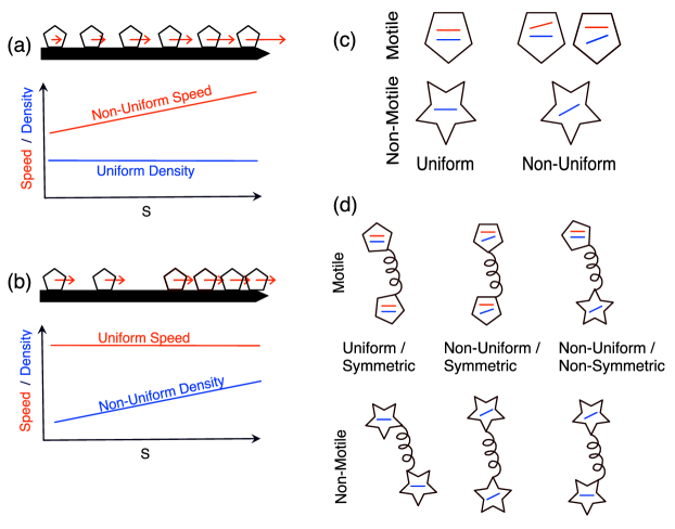
Figure 2: (a, b) Populations of crosslink heads are characterized by the density with which they bind a filament along its arclength $s$ and the speed at which they move when force free. Two different head types, one with non-uniform speed but uniform density (a) another with uniform speed and non-uniform density (b) are shown. In (c) we list some possible crosslink heads. Red and Blue lines illustrate the change of crosslink speed and density with $s$, respectively. In (d) we illustrate example crosslinks which consist of two heads and a linker.

The coefficients in Eq. (35) arise from a distribution of active and passive crosslinks that act between filaments. Consider an ensemble of crosslinking molecules, each consisting of two heads $a$ and $b$, joined by a spring-like linker; see Fig. (2). For any small volume in an active network, we can count the number densities $\xi_{a}(s)$, and $\xi_{b}(s)$ of $a$ and $b$ heads of doubly-bound crosslinks that are attached to a filament at arc-length position $s$. In an idealized experiment $\xi_{a}(s)$ and $\xi_{b}(s)$ could be determined by recording the positions of motor heads on filaments. The number-density $\xi_{ab}(s_{i},s_{j})$ of $a$ heads at position $s_{i}$ on microtubule $i$ connected to $b$ heads at position $s_{j}$ on microtubule $j$ is then given by

$$\xi_{ab}(s_{i},s_{j})=\frac{\xi_{a}(s_{i})\xi_{b}(s_{j})}{N_{b}^{(i)}(s_{i})}$$ (67)

where $N^{(i)}_{b}(s_{i})$ counts the $b$ heads that an $a$-head attached at position $s_{i}$ on filament $i$ could be connected to given the crosslink size. It obeys

$$N^{(i)}_{b}(s_{i})=\sum\limits_{k\neq i}\int\limits_{-L/2}^{L/2}ds_{k}\int\limits_{\Omega(\mathbf{x}_{i}+s_{i}\mathbf{p}_{i})}d\mathbf{x}^{3}\xi_{b}(s_{k})\delta(\mathbf{x}_{k}+s_{k}\mathbf{p}_{k}-\mathbf{x}).$$ (68)

Analogous definitions for $\xi_{ba}(s_{i},s_{j})$ and $N_{a}^{(i)}(s_{i})$ are implied. It follows naturally that $\xi(s_{i},s_{j})=\xi_{ab}(s_{i},s_{j})+\xi_{ba}(s_{i},s_{j})$ is the total number density of crosslinks acting between filaments $i$ and $j$ at the arclength positions $s_{i}$, $s_{j}$.

Now let $V_{a}(s),V_{b}(s)$ be the load-free velocities of motor-heads $a,b$ moving along filaments. Here, $V_{a}(s),V_{b}(s)$ are functions of the arc-length position $s$. Like $\xi_{a}$ and $\xi_{b}$, they are in principle measurable. With these definitions, the force per unit surface that attached motors exert is

$$\mathbf{f}_{ij}=-\Gamma\xi(s_{i},s_{j})\left(\mathbf{v}_{i}+s_{i}\dot{\mathbf{p}}_{i}-\mathbf{v}_{j}+s_{j}\dot{\mathbf{p}}_{j}\right)$$

$$-\kappa\xi(s_{i},s_{j})\left(\mathbf{x}_{i}+s_{i}\mathbf{p}_{i}-\mathbf{x}_{j}+s_{j}\mathbf{p}_{j}\right)$$

$$-\Gamma\left(\left[\xi_{ab}(s_{i},s_{j})V_{a}(s_{i})+\xi_{ba}(s_{i},s_{j})V_{b}(s_{i})\right]\mathbf{p}_{i}\right)$$

$$+\Gamma\left(\left[\xi_{ab}(s_{j},s_{i})V_{a}(s_{j})+\xi_{ba}(s_{j},s_{i})V_{b}(s_{j})\right]\mathbf{p}_{j}\right),$$ (69)

where $\Gamma$ is an effective linear friction coefficient between the two attachment points and $\kappa$ is an effective spring constant. They depend on the microscopic properties of motors, filaments, and the concentrations of both and their regulators. In general, $\Gamma$ and $\kappa$ are second rank tensors, which depend on the relative orientations of filaments. Here we take them to be scalar, for simplicity and consistency with earlier assumptions. By comparing to Eq. (35) we identify

$$\gamma(s_{i},s_{j})=-\Gamma\xi(s_{i},s_{j}),$$ (70)

$$K(s_{i},s_{j})=-\kappa\xi(s_{i},s_{j}),$$ (71)

and

$$\sigma(s_{i},s_{j}) = -\Gamma\xi_{ab}(s_{i},s_{j})V_{a}(s_{i})+\Gamma\xi_{ba}(s_{i},s_{j})V_{b}(s_{i}).$$ (72)

	$\gamma_{0}$, $K_{0}$	$\gamma_{1}$, $K_{1}$	$\sigma_{0}$	$\sigma_{10}$	$\sigma_{01}$
symmetric uniform non-motile	yes	no	no	no	no
non-symmetric uniform non-motile	yes	yes	no	no	no
symmetric uniform motor	yes	no	yes	no	no
symmetric non-uniform motor	yes	yes	yes	yes $\sigma_{10}=\sigma_{1}$	yes $\sigma_{01}=\sigma_{1}$
non-symmetric non-uniform motor	yes	yes	yes	yes	yes

Table 1: Table summarizing which crosslink moments different crosslink types generate.

Using Eqs. (70, 71, 72), we now discuss some important classes of crosslinking molecules. We consider crosslinks whose heads can be motile or non-motile, the binding and walking properties can act uniformly or non-uniformly along filaments, and the two heads of the crosslink can be the same (symmetric crosslink) or different (non-symmetric crosslink). Figure 2 maps how varying crosslink types can be constructed, while Table 1 lists the moments to which different classes of crosslinks contribute.

Non-motile crosslinks are crosslinks that do not actively move, i.e. $V_{a}=V_{b}=0$. Examples of non-motile crosslinks in cytoskeletal systems are the actin bundlers such as fascin, or microtubule crosslinks such as Ase1p alberts_2002_book . While these types of crosslinks are not necessarily passive, since the way they binding or unbind can break detailed balance, that their attached heads do not walk along filaments implies that $\sigma_{0}=\sigma_{10}=\sigma_{01}=0$. Non-motile crosslinks change the material properties of the material by contributing to the crosslink moments $\gamma_{0},\gamma_{1}$ and $K_{0},K_{1}$. Some non-motile crosslinks bind non-specifically along filaments they interact with, giving uniform distributions. For these $\gamma_{1}=K_{1}=0$. Others preferentially associate to filament ends, and thus bind non-uniformly. For these $\gamma_{1}$ and $K_{1}$ are positive. Note that the two heads of a non-motile crosslink can be identical (symmetric) or not (non-symmetric). Given the symmetric structure of Eqs (70, 71) mechanically a non-symmetric non-motile crosslink behaves the same as a symmetric non-motile crosslink. and Symmetric Motor crosslinks are motor molecules whose two heads have identical properties, i.e. $V_{a}=V_{b}=V$ and $\xi_{a}=\xi_{b}=\xi$. Examples are the microtubule motor molecule Eg-5 kinesin, and the Kinesin-2 motor construct popularized by many in-vitro experimentssanchez2012spontaneous . Symmetric motors contribute to the large-scale properties of the material by generating motor forces. In particular they contribute to the crosslink moments $\sigma_{0}$, $\sigma_{10}$, and $\sigma_{01}$. From Eq. (72) it is easy to see that $\sigma_{0}=V_{0}\gamma_{0}+V_{1}\gamma_{1}/L^{2}$, where we defined the moments of the motor velocity $V(s_{i},s_{j})$ using Eq. (36). Some symmetric motor proteins preferentially associate to filament ends, and display end-clustering behavior, where their walking speed depends on the position at which they are attached to filaments. Motors that do either of these also generate a contribution to $\sigma_{10}$ and $\sigma_{01}$. Since both motor heads are identical we have $\sigma_{10}=\sigma_{01}\equiv\sigma_{1}$ and from Eq. (72) we find that $\sigma_{1}=\gamma_{1}V_{0}+V_{1}\gamma_{0}$.

Non-Symmetric motor crosslinks are motor molecules whose two heads have differing properties. An example is the microtubule-associated motor dynein, that consists of a non-motile end that clusters near microtubule minus-ends and a walking head that binds to nearby microtubules whenever they are within reach foster2015active ; foster2017connecting . A consequence of motors being non-symmetric is that $\sigma_{10}\neq\sigma_{01}$. Since non-symmetric motors can break the symmetry between the two heads in a variety of ways we spell out the consequences for a few cases. Let us first consider a crosslinker with one head $a$ that acts as a passive crosslink ($V_{a}=0$) and a second head $b$ that acts as a motor, moving with the stepping speed $V_{b}=V$. For such a crosslink $\sigma_{0}=\gamma_{0}V_{0}/2$. If both heads are distributed uniformly along filaments and their $V$ is position independent then $\sigma_{01}=\sigma_{10}=0$. If the walking $b$-head is distributed nonuniformly ($\xi_{b}=\xi_{b}(s),\xi_{a}=$ constant) then $\sigma_{10}=\gamma_{1}V_{0}$ and $\sigma_{01}=0$. Conversely, if the static $a$-head has a patterned distribution ($\xi_{a}=\xi_{a}(s),\xi_{b}=$ constant) then $\sigma_{01}=\gamma_{1}V_{0},\sigma_{10}=0$. Finally, we note that if both heads are distributed uniformly along the filament ($\xi_{a}=\xi_{b}=$constant), but the walking $b$-head of the motor changes its speed as function of position then $\sigma_{10}=V_{1}\gamma_{0}/2$ and $\sigma_{01}=0$.

Note that stresses and forces are additive. Thus it may be possible to design specific crosslink moments by designing mixtures of different crosslinkers. For instance mixing a non-motile crosslink that has specific binding to a filament solution might allow to change just $\gamma_{0}$ and $\gamma_{1}$ in a targeted way. We will elaborate on some of these possibilities in what follows.

V.2 Tuning viscosity

We now discuss how microscopic processes shape the overall magnitude of the viscosity tensor $\chi$. From Eq. (64) and remembering that $\eta=3R^{2}/10\gamma_{0}$, it is apparent that the overall viscosity of the material is proportional to the number of crosslinking interactions and their resistance to the relative motion of filaments, quantified by the friction coefficient $\rho^{2}\gamma_{0}$. Furthermore, $\gamma_{0}$ itself scales as the squared filament length $L$, and the cubed crosslink size $R$ (see the definition in Appendix B), which, with $\rho^{2}$, sets the overall scale of the viscosity as $\rho^{2}L^{2}R^{3}$.

We next show how micro-scale properties of network constituents shape the anisotropy of $\chi$ ; see Eq. (64). To characterize this we define the anisotropy ratio $a$ as

$$a=\frac{L^{2}\gamma_{0}}{12\eta}=\frac{5}{18}\frac{L^{2}}{R^{2}},$$ (73)

which is the ratio of the magnitudes of the isotropic part of $\chi_{\alpha\beta\gamma\mu}$, that is $\eta\delta_{\alpha\gamma}\delta_{\beta\mu}$, and its anisotropic part $\gamma_{0}L^{2}/12(\mathcal{Q}_{\alpha\gamma}\delta_{\beta\mu}-\mathcal{S}_{\alpha\beta\gamma\mu})$. Most apparently the anisotropy ratio will be large if the typical filament length $L$ is large compared to the motor interaction range $R$. This is typically the case in microtubule based systems, as microtubules are often microns long and interact via motor groups that are a few tens of nano-meters in scale alberts_2002_book . Conversely, in actomyosin systems filaments are often shorter (hundreds of nano-meters) and motors-clusters called mini-filaments, can have sizes similar to the filament lengths alberts_2002_book . The anisotropy of the viscous stress is not exclusive to active systems and has been described before in the context of similar passive systems, such as liquid crystals and liquid crystal polymers de1993physics ; chaikin2000principles ; doi1988theory .

V.3 Tuning the active self-strain

Mixture	Active Strain, $\sigma_{0}/\gamma_{0}$	Active Pressure, $\Pi^{\mathrm{(A)}}$ Axial stress, $\bar{S}$
	$\frac{\sigma_{0}}{\gamma_{0}}=V_{0}$	no
	$\frac{\sigma_{0}}{\gamma_{0}}=V_{0}$	no
	$\frac{\sigma_{0}}{\gamma_{0}}=\frac{V^{a}_{0}+V^{b}_{0}}{2}$
+		no
+ or +

Table 2: Active pressure and strain generated by different crosslink types and mixtures. In the plots pertaining to the active strain rate $\gamma_{0}=\gamma_{0}^{(M)}+\gamma_{0}^{(X)}$ where $\gamma_{0}^{(M)}$ denotes the is the part of $\gamma_{0}$ induced by mobile and $\gamma_{0}^{(X)}$ denotes contribution from non-mobile crosslinkers. The filament sliding velocity expected in a stress free system is $V_{slide}=\sigma_{0}/\gamma_{0}$ and is given units of the force free speed of immobile crosslinks and describe the expected speed of filament sliding in the material. Moreover, $\bar{S}=|\Pi^{\mathrm{(A)}}/q|$ is the magnitude of the motor-stepping induced axial stress, i.e of the axial stress in the limit $K_{0}\to 0$.

The viscous stress in highly crosslinked networks is given by $\chi:\mathcal{U}$, where $\mathcal{U}=\nabla\mathbf{v}+(\sigma_{0}/\gamma_{0})\nabla\mathbf{P}$ takes the role of the strain-rate in passive materials, but with an active contribution $(\sigma_{0}/\gamma_{0})\nabla\mathbf{P}$. Thus, internally driven materials can exhibit active self-straining.

In particular a material in which each filament moves with the velocity $\mathbf{v}_{i}=-\sigma_{0}/\gamma_{0}\mathbf{p}_{i}+\mathbf{C}$, where $\mathbf{C}$ is a constant vector that is sets the net speed of the material in the frame of reference, has $\mathcal{U}=0$, and thus zero viscous stress. In such a material filaments can slide past each other at a speed $\sigma_{0}/\gamma_{0}$ without stressing the material. Notably, the sliding speed is independent of the local polarity and nematic order of the material furthauer2019self .

The crosslink moments that contribute to the active straining behavior are $\sigma_{0}$ and $\gamma_{0}$. In active filament networks with a single type of crosslink $\sigma_{0}/\gamma_{0}\simeq V_{0}$, regardless of crosslink concentration. Thus for single-crosslinker systems, the magnitude of self-straining is independent of the motor concentration furthauer2019self .

Self-straining can be tuned in mixtures of crosslinks. For instance the addition of a non-motile crosslinker can increase $\gamma_{0}$, while leaving $\sigma_{0}$ unchanged. In this way self-straining can be relatively suppressed. In table 2 we plot the expected active strain-rate for materials actuated by mixtures of immotile and motor crosslinks. In such a material $\gamma_{0}=\gamma_{0}^{(M)}+\gamma_{0}^{(X)}$ where $\gamma_{0}^{(M)}$ denotes the part of $\gamma_{0}$ induced by motile crosslinkers and $\gamma_{0}^{(X)}$ denotes that from non-motile crosslinkers. The resulting velocity $V_{slide}$ with which a filament slides through the material will scale as $V_{slide}\simeq\gamma_{0}^{(M)}/(\gamma_{0}^{(M)}+\gamma_{0}^{(X)})$; see Table 2.

V.4 Tuning the Active Pressure

Many active networks spontaneously contract foster2015active or expand sanchez2012spontaneous . We now study the motor properties that enable these behaviors.

An active material with stress free boundary conditions, can spontaneously contract if its self-pressure,

$$\Pi=\mathrm{Tr}\left(\mathbf{\Sigma}+\rho^{2}\chi:\mathcal{U}\right).$$ (74)

is negative. Conversely the material can spontaneously extend if $\Pi$ is positive. We can also write

$$\Pi=\Pi^{\mathrm{(A)}}+\Pi^{\mathrm{(S)}}$$ (75)

where $\Pi^{\mathrm{(S)}}=\mathrm{Tr}\left(\mathbf{\Sigma}^{\mathrm{(S)}}\right)$ is the sterically mediated pressure, and $\Pi^{\mathrm{(A)}}$ is the activity driven pressure (or active pressure) given by

$$\Pi^{\mathrm{(A)}}=-\rho^{2}\left(\alpha K_{0}+A^{(\mathcal{Q})}-A^{(\mathbf{P})}|\mathbf{P}|^{2}\right).$$ (76)

see Eq. (63). Here and in the following we approximated $\mathrm{Tr}(\mathcal{T}\cdot\mathbf{P})\simeq|\mathbf{P}|^{2}$ for simplicity. We ask which properties of crosslinks set the active pressure and how its sign can be chosen.

We first discuss how interaction elasticity impacts the active pressure $\Pi^{(A)}$ in the absence of motile crosslinks, i.e. when $\sigma_{0}=\sigma_{10}=\sigma_{01}=0$. In this case, Eq. (76) simplifies to $\Pi^{\mathrm{(A)}}=-\rho^{2}(\alpha+L^{2}/12)K_{0}$, where we used Eq. (65). Thus, even in the absence of motile crosslinks, active pressure can be generated. This can be tuned by changing the effective spring constant $K_{0}$. We note that $\Pi^{\mathrm{(A)}}+\Pi^{\mathrm{(S)}}=0$ when crosslink binding-unbinding obeys detailed balance and the system is in equilibrium. The moment $K_{0}$ can have either sign when detailed balance is broken. Microscopically this effect could be achieved, for instance, by a crosslinker in which active processes change the rest length of a spring-like linker between the two heads once they bind to filaments.

We next discuss the contributions of motor motility to the active pressure. To start, we study a simplified apolar (i.e. $\mathbf{P}=0$) system where $K=0$. In such a system the active pressure is given by

$$\Pi^{\mathrm{(A)}}=-\rho^{2}\left(\sigma_{10}-\sigma_{0}\frac{\gamma_{1}}{\gamma_{0}}\right)$$ (77)

We ask how motor properties set the value and sign of this parameter combination.

We first point out that generating active pressure by motor stepping requires that either $\sigma_{10}$ or $\gamma_{1}$ are non-zero. This means that generating active pressure requires breaking the uniformity of binding or walking properties along the filament. A crosslink which has two heads that act uniformly can thus not generate active pressure on its own. However, when operating in conjunction with a passive crosslink that preferentially binds either end of the filament, the same motor can generate an active pressure. This pressure will be contractile if the non-motile crosslinks couple the end that the motor walks towards ($\gamma_{1}$ and $\sigma_{0}$ have the same sign) and extensile if they couple the other ($\gamma_{1}$ and $\sigma_{0}$ have opposite signs). In summary, a motor crosslink that acts the same everywhere along the filaments it couples does not generate active pressure on its own. However, it can do so when mixed with a passive crosslink that acts non-uniformly.

We next ask if a system with just one type of non-uniformly acting crosslink can generate active pressure. To start, consider symmetric motor crosslinks, i.e a motor consisting of two heads with identical (but non-uniform) properties. We then have $\sigma_{01}=\sigma_{10}=\gamma_{1}V_{0}+\gamma_{0}V_{1}$ and $\sigma_{0}=V_{0}\gamma_{0}+V_{1}\gamma_{1}/L^{2}$. Using this in Eq. (77) and dropping the term proportional to $\gamma_{1}^{2}$ (higher order in this case) we find that such symmetric motor crosslinks generate no contribution to the active pressure when operating alone. However when operating in concert with a non-motile crosslink, even one that binds filaments uniformly, they can generate and active pressure. The sign of the active pressure is set by the particular asymmetry of motor binding and motion. The system is contractile if motors cluster or speed up near the end towards which they walk, and extensile if they cluster or accelerate near the end that they walk from. Our prediction that many motor molecules can only generate active pressure in the presence of an additional crosslink, might explain observation on acto-myosin gels, which have been shown to contract only when combined a passive crosslink operate in concert with the motor myosin ennomani2016architecture .

We next ask if non-symmetric motor crosslinks can generate active pressure. Consider a crosslink with one immobile and one walking head. For such a crosslink $\sigma_{0}=\gamma_{0}V_{0}/2$. If the immobile head preferentially binds near one filament end, while the walking head attaches everywhere uniformly, then $\sigma_{10}=\gamma_{1}V_{0}$ and $\sigma_{01}=0$. For such a motor we predict an active pressure proportional to $V_{0}/2$. The active pressure will be contractile if the static ends bind near the end that the motor head walks to and extensile if the situation is reversed. The motor dynein has been suggested to consist of an immobile head that attaches near microtubule minus ends and a walking head that grabs other microtubules and walks towards their minus ends. Our theory suggests that this should lead to contractions, which is consistent with experimental findings ennomani2016architecture .

After having discussed the effects of motor stepping on the active pressure in systems with $\mathbf{P}=0$, we ask how the situation changes in polar systems. In polar system an additional contribution, $-(\sigma_{01}-\frac{\gamma_{1}}{\gamma_{0}}\sigma_{0})|\mathbf{P}|^{2}$, exists. For symmetric motors, where $\sigma_{01}=\sigma_{10}$ this implies that the active pressure generated by a network of symmetric motors and passive crosslinks is strongest in apolar regions of the system and subsides in polar regions, since the polar and apolar contributions to the active stress appear in Eq. (63) with opposite signs. We plot the magnitude of the active pressure $\Pi^{\mathrm{(A)}}\simeq 1-|\mathbf{P}|^{2}$ as a function of $|\mathbf{P}|$ in Table 2. This is reminiscent of the behavior predicted in the frameworks of a sparsely crosslinked system in gao2015multiscalepolar . In contrast the effects of non-symmetric motors can be enhanced in polar regions. Consider again, the example of a motor with one static head that preferentially binds near one of the filament ends and a mobile head that acts uniformly. For this motor $\sigma_{10}=\gamma_{1}V_{0}$ and $\sigma_{01}=0$ and $\sigma_{0}=\gamma_{0}V_{0}/2$. It is thus predicted to generate twice the amount of active pressure in a polar network than in an apolar one and $\Pi^{\mathrm{(A)}}\simeq(1+|\mathbf{P}|)/2$, see the table 2 for a plot of the active pressure $\Pi^{\mathrm{(A)}}$ as a function of $|\mathbf{P}|$. This is reminiscent of the motor dynein in spindles, which is though to generate the most prominent contractions near the spindle poles, which are polar brugues2012nucleation .

Finally, we ask how filament length affects the active pressure. Looking at the definitions of the nematic and polar activity Eqs. (65, 61) and remembering the definition and scaling of the coefficient in there (see App. (B)), we notice that the active pressure scales as $L^{4}$. Since the viscosity scaled with $L^{2}$, this predicts that systems with shorter filaments contract slower than systems with longer filaments. This effect has observed for dynein based contractions in-vitro foster2017connecting .

V.5 Tuning axial stresses, buckling and aster formation

Motors in active filament networks generate anisotropic (axial) contributions to the stress, which can lead to large scale instabilities in materials with nematic order simha2002hydrodynamic ; kruse2005generic ; saintillan2008instabilitiesPRL ; furthauer2012taylor . At larger active stresses, nematics are unstable to splay deformations in systems that are contractile along the nematic axis, and to bend deformations in systems that are extensile along the nematic axis kruse2005generic ; marchetti2013hydrodynamics . In both cases, the instabilities set in when the square root of ratio of the elastic (bend or splay) modulus that opposes the deformation to the active stress - also called the Fréedericksz length - becomes comparable to the systems size. We now discuss which motor properties control the emergence of these instabilities, and how a system can be tuned exhibit bend or splay deformations. For this we ask how axial stresses, which are governed by the activity parameters $\mathcal{A}^{(\mathcal{Q})}$ and $\mathcal{A}^{(\mathbf{P})}$, are set in our system.

The magnitude $S$ of the axial stress along the nematic axis is given by

$$S=-\rho^{2}q\left(\mathcal{A}^{(\mathcal{Q})}-\mathcal{A}^{(\mathbf{P})}|\mathbf{P}|^{2}\right),$$ (78)

where we defined the nematic order parameter $q$, as the largest eigenvalue of ${\mathcal{Q}}-\mathrm{Tr}(\mathcal{Q})\mathcal{I}/3$; see Eq. (63). The axial stress is contractile along the nematic axis if $S$ is positive and extensile if $S$ is negative. Comparing Eqs. (78, 76) we find that $S=q(\Pi^{\mathrm{(A)}}+\rho^{2}\alpha K_{0})$ and in the limit where $K_{0}\to 0$, where motor elasticity is negligible, $S=q\Pi^{\mathrm{(A)}}$. We discussed how $\Pi^{\mathrm{(A)}}$ is set for different types of crosslinks in the previous section; see Table 2.

The prototypical active nematic sanchez2012spontaneous which consists of apolar bundles of microtubules actuated by the kinesin motors and is axial extensile. In our theory, an axial extensile stress (i.e. $S<0$) in an apolar system ($\mathbf{P}=0$) implies that $\mathcal{A}^{(\mathcal{Q})}=\sigma_{10}-\sigma_{0}\frac{\gamma_{1}}{\gamma_{0}}+\frac{L^{2}}{12}K_{0}>0$. This can be achieved either by crosslinks that act uniformly (i.e. $\sigma_{10}-\sigma_{0}\frac{\gamma_{1}}{\gamma_{0}}=0$) and generate a spring like response that induces $K_{0}>0$ or by crosslinks that have non-uniform motor stepping behavior which generates $\sigma_{10}-\sigma_{0}\frac{\gamma_{1}}{\gamma_{0}}>0$. The latter implies either a non-symmetric motor crosslinks, or the presence of more than one kind of crosslinks, as was discussed more extensively earlier in the context of active pressure. At high enough active stress we expect systems with negative $S$ to become unstable towards buckling. This has been observed in senoussi2019tunable ; strubing2019wrinkling .

Conversely axial contractile behavior can be achieved if either $K_{0}<0$ or $\sigma_{10}-\sigma_{0}\frac{\gamma_{1}}{\gamma_{0}}<0$. At high enough active stress, such systems can become unstable towards an aster forming transition, as seen in foster2015active .

Note that $S\simeq\Pi^{\mathrm{(A)}}+\rho^{2}\alpha K_{0}$, implies that $S$ and $\Pi^{\mathrm{(A)}}$ need not be the same if $K_{0}\neq 0$. In particular when $\Pi^{\mathrm{(A)}}$ and $K_{0}$ have opposite signs systems can exist, which are axially extensile while being bulk contractile and vice versa.

We finally note that the magnitude of axial stresses changes if the system transitions from apolar to polar, if the origin of the axial stresses is motor stepping but not if the origin of the axial stresses is the effective spring like behavior of motor, since $\mathcal{A}^{(\mathcal{Q})}$, but not $\mathcal{A}^{(\mathbf{P})}$, depends on $K_{0}$, see Eqs. (61, 65). In systems in which the active stress is generated by the stepping of symmetric motor-crosslink, $|S|$ is highest nematic apolar phase ($|\mathbf{P}|=0$), while systems made from non-symmetric crosslinks generate the most stress when polar ($|\mathbf{P}|=1$); see Table 2. This opens the possibility that a system can overcome the threshold towards an instability when its other dynamics drives it from nematic apolar to polar arrangements or vice versa. We suggest that the buckling instabilities discussed in senoussi2019tunable ; strubing2019wrinkling should be interpreted in this light.

VI Discussion

In this paper, we asked how the properties of motorized crosslinkers that act between the filaments of a highly crosslinked polymer network set the large scale properties of the material.

For this, we first develop a method for quantitatively stating what the properties of motorized crosslinks are. We introduce a generic phenomenological model for the forces that crosslink populations exert between the filaments which they connect; see Eq. (35). This model describes forces that are (i) proportional to the distance ($K$), and (ii) the relative rate of displacement ($\gamma$). Finally (iii) it describes the active motor forces ($\sigma$) that crosslinks can exert. Importantly, forces from crosslinkers ($K,\gamma,\sigma$) can depend on the position on the two filaments which they couple. This allows the description of a wide range of motor properties, such as end-binding affinity, end-dwelling, and even the description of non-symmetric crosslinks that consist of motors with two heads of different properties.

We next derived the stresses and forces generated on large time and length scale, given our phenomenological crosslink model. We find that the emergent material stresses depend only on a small set of moments; see Eq. (36) of the crosslink properties. These moments are effectively descriptions of the expectation value of the force exerted between two filaments given their positions and relative orientations. The resulting stresses, forces, and filament reorientation rates (Eqs. (63, 62, 59)) recover the symmetries and structure predicted by phenomenological theories for active materials, but beyond that provide a way of identifying how specific micro-scale processes set specific properties of the material.

We discussed how four key aspects of the dynamics of highly crosslinked filament networks can be tuned by the micro-scale properties of motors and filaments. In particular we discussed how (i) the highly anisotropic viscosity of the material is set; (ii) how active self-straining is regulated; (iii) how contractile or extensile active pressure can be generated; (iv) which motor properties regulate the axial active nematic and bipolar stresses, which can lead to large scale instabilities.

Our theory makes specific predictions for the effects of distinct classes of crosslinkers on cytoskeletal networks. Intriguingly these predictions suggest explanations for phenomena experimentally seen, but currently poorly understood.

Experiments have shown that mixtures of actin filaments and myosin molecular motors can spontaneously contract, but only in the presence of an additional passive crosslinker ennomani2016architecture . Our theory allows us to speculate on explanations for this observation. In the crosslink classification that we introduced, myosin, which form large mini-filaments, is a symmetric motor crosslink; see Fig. (2). We find that symmetric motor crosslinks, which have two heads that act the same can generate contractions only in the presence of an additional crosslinker that helps break the balance between $\gamma_{1}/\gamma_{0}\sigma_{0}$ and $\sigma_{01}$ in the active pressure; see Eq. (77) and Table 2. Further work will be needed to explore whether this connection can be made quantitative.

A second observation that was poorly understood prior to this work is the sliding motion of microtubules in meiotic Xenopus spindles, which are the structures which segregate chromosomes during the meiotic cell division. These spindles consist of inter-penetrating arrays of anti-parallel microtubules, which are nematic near the chromosomes, and highly polar near the spindle poles. In most of the spindle the two anti-parallel populations of microtubules slide past each other, at near constant speed driven by the molecular motor Eg-5 Kinesin, regardless of the local network polarity. Our earlier work furthauer2019self showed that active self straining explains this polarity independent motion. The theory that we develop here provides the tools to explore the behavior of different motors and motor mixtures which will allow us to investigate the mechanism by which different motors in the spindle shape its morphology. This will help to explain complex behaviors of spindles such as the barreling instability oriola2020active that gives spindles their characteristic shape or the observation that spindles can fuse gatlin2009spindle .

Our theory provides specific predictions on how changing motor properties can change the properties of the material which they constitute, it can enable the design of new active materials. We predict the expected large scale properties of a material, in which an experimentalist had introduced engineered crosslinks with controlled properties. With current technology, an experimentalist could engineer a motor that preferentially attaches one of its heads to a specified location on a filament, while its walking head reaches out into the network. Or, as has already been demonstrated in studies by the Surrey Lab roostalu2018determinants the difference in the rates of filament growth and motor walking speeds, could be exploited to generate different dynamic motor distributions on filaments. This design space will provide ample room to experimentally test our predictions, and use them to engineer systems with desirable properties. Finally recent advances in optical control of motor systems ross2019controlling could be used to provide spatial control.

The theory presented here does however make some simplifications. Importantly, we neglected that the distribution of bound crosslinks on filaments themselves in general depends on the configuration of the network. This means that the crosslink moments can themselves be functions of the local network order parameters. Effects like this have been argued to be important for instance when explaining the transition from contractile to extensile stresses in ordering microtubule networks lenz2020reversal and the physics of active bundles kruse2003self . Such effects can be recovered when making the interactions $K,\gamma,\sigma$ in the phenomenological crosslink force model Eq. (35) functions of $\mathbf{p}_{i}$, and $\mathbf{p}_{j}$. This will be the topic of a subsequent publication.

In summary, in this paper we derived a continuum theory for systems made from cytoskeletal filaments and motors in the highly crosslinked regime. Our theory makes testable predictions on the behavior of the emerging system, provides a unifying framework in which dense cytoskeletal systems can be understood from the ground up, and provides the design paradigms, which will enable the creation of active matter systems with desirable properties in the lab.

Acknowledgements We thank Meridith Betterton and Adam Lamson for insightful discussions. We also thank Peter J. Foster and James F. Pelletier for feedback on the manuscript. DN acknowledges support by the National Science Foundation under awards DMR-2004380 and DMR-0820484. MJS acknowledges support by the National Science Foundation under awards DMR-1420073 (NYU MRSEC), DMS-1620331, and DMR-2004469.

Appendix A Detailed derivation of the equations of motion

In the following we derive the equations of motion for the highly crosslinked active network. We start by using Eq. (55, 34) and obtain

$$\dot{\mathbf{p}}_{i} = \left(\mathcal{I}-\mathbf{p}_{i}\mathbf{p}_{i}\right)\cdot\left\{\mathbf{p}_{i}\cdot(\mathcal{U}+\frac{12}{\gamma_{0}L^{2}}\frac{\mathcal{E}}{\rho^{2}})+\frac{12}{\gamma_{0}L^{2}}A^{(\mathbf{P})}\mathbf{P}\right\}$$ (79)

$$- \frac{1}{\rho}\bar{\mathbf{T}}_{i}^{\mathrm{(drag)}},$$

The torque due to drag with the medium is

$$\bar{\mathbf{T}}^{(drag)}_{i}={\mathbf{T}}^{(drag)}_{i}$$

$$+ \left(\mathcal{I}-\mathbf{p}_{i}\mathbf{p}_{i}\right)\cdot\left(\frac{12}{\gamma_{0}L^{2}}+\mathbf{p}_{i}\cdot\frac{\nabla\rho}{\rho}\right)\left(\mathbf{F}_{i}^{\mathrm{(drag)}}-\frac{1}{\rho}\mathbf{f}\right).$$

This implies

$$\mathbf{\omega} = \mathbf{P}\cdot(\mathcal{U}+\frac{12}{\gamma_{0}L^{2}}\frac{\mathcal{E}}{\rho^{2}})-\mathcal{T}:(\mathcal{U}+\frac{12}{\gamma_{0}L^{2}}\frac{\mathcal{E}}{\rho^{2}})$$

$$+ \frac{12}{L^{2}}A^{(\mathbf{P})}\left(\mathbf{P}-\mathcal{Q}\cdot\mathbf{P}\right)-\frac{1}{\rho}\omega^{\mathrm{(drag)}},$$

where

$$\omega^{\mathrm{(drag)}}=\left<\bar{\mathbf{T}}^{(drag)}_{i}\right>$$ (82)

and

$$\mathcal{H} = \mathcal{Q}\cdot(\mathcal{U}+\frac{12}{\gamma_{0}L^{2}}\frac{\mathcal{E}}{\rho^{2}})-\mathcal{S}:(\mathcal{U}+\frac{12}{\gamma_{0}L^{2}}\frac{\mathcal{E}}{\rho^{2}})$$ (83)

$$+ \frac{12}{\gamma_{0}L^{2}}A^{(\mathbf{P})}\left(\mathbf{P}\mathbf{P}-\mathcal{T}\cdot\mathbf{P}\right)$$

$$- \frac{1}{\rho}\mathcal{H}^{\mathrm{(drag)}},$$

where

$$\mathcal{H}^{\mathrm{(drag)}}=\left<\mathbf{p}_{i}\bar{\mathbf{T}}^{(drag)}_{i}\right>.$$ (84)

Furthermore we note that

$$\mathbf{j}=\frac{\sigma_{0}}{\gamma_{0}}(\mathbf{P}\mathbf{P}-\mathcal{Q})+\frac{1}{\gamma_{0}\rho}\mathbf{j}^{\mathrm{(drag)}}+\mathcal{O}\left(L^{2}\right),$$ (85)

and

$$\mathcal{J}=\frac{\sigma_{0}}{\gamma_{0}}(\mathcal{Q}\mathbf{P}-\mathcal{T})+\frac{1}{\gamma_{0}\rho}\mathcal{J}^{\mathrm{(drag)}}+\mathcal{O}\left(L^{2}\right),$$ (86)

where

$$\mathbf{j}^{\mathrm{(drag)}}=-\frac{1}{\gamma_{0}}\left<\mathbf{p}_{i}\left(\mathbf{F}_{i}^{\mathrm{(drag)}}-\frac{1}{\rho}\mathbf{f}\right)\right>$$ (87)

and

$$\mathcal{J}^{\mathrm{(drag)}}=-\frac{1}{\gamma_{0}}\left<\mathbf{p}_{i}\mathbf{p}_{i}\left(\mathbf{F}_{i}^{\mathrm{(drag)}}-\frac{1}{\rho}\mathbf{f}\right)\right>.$$ (88)

Putting all of this together, we arrive at an expression for the networks stress in terms of the current distribution of filaments,

$$\mathbf{\Sigma} = -\rho^{2}\left(\chi:\mathcal{U}+\alpha K_{0}\mathcal{I}\right)$$

$$- \rho^{2}\left(A^{(\mathcal{Q})}\mathcal{Q}-A^{(\mathbf{P})}\mathcal{T}\cdot\mathbf{P}\right)$$

$$- \bar{\chi}:\mathcal{E}+\bar{\mathbf{\Sigma}}+\rho\mathbf{\Sigma}^{\mathrm{(drag)}}.$$

where

$$\mathbf{\Sigma}^{\mathrm{(drag)}}=-\gamma_{0}\frac{L^{2}}{12}\mathcal{H}^{\mathrm{(drag)}}-\gamma_{1}\mathbf{j}^{\mathrm{(drag)}}$$ (90)

and at a similar equation for the motion of filament $i$

$$\mathbf{v}_{i}-\mathbf{v} = -\frac{\sigma_{0}}{\gamma_{0}}\left(\mathbf{p}_{i}-\mathbf{P}\right)$$

$$- \frac{\gamma_{1}}{\gamma_{0}}\left(\begin{array}[]{c}(\mathbf{p}_{i}-\mathbf{P})\cdot(\mathcal{U}+\frac{12}{\gamma_{0}L^{2}}\frac{\mathcal{E}}{\rho^{2}})\\ -(\mathbf{p}_{i}\mathbf{p}_{i}\mathbf{p}_{i}-\mathcal{T}):(\mathcal{U}+\frac{12}{\gamma_{0}L^{2}}\frac{\mathcal{E}}{\rho^{2}})\end{array}\right)$$

$$+ \frac{1}{\gamma_{0}}\frac{12\gamma_{1}}{L^{2}\gamma_{0}}A^{(\mathbf{P})}\left(\mathbf{p}_{i}\mathbf{p}_{i}-\mathcal{Q}\right)\cdot\mathbf{P}$$

$$- \frac{\nabla\rho}{\gamma_{0}\rho}\cdot\left[\begin{array}[]{c}A^{\mathcal{Q}}\left(\mathbf{p}_{i}\mathbf{p}_{i}-\mathcal{Q}\right)\\ -A^{(\mathbf{P})}\left(\mathbf{p}_{i}\mathbf{P}+\mathbf{P}\mathbf{p}_{i}-2\mathbf{P}\mathbf{P}\right)\end{array}\right]$$ (96)

$$- \left(\mathbf{p}_{i}\mathbf{p}_{i}-\mathcal{Q}):\nabla\frac{\mathcal{E}}{\rho}\right)-\frac{1}{\rho}\mathbf{v}^{\mathrm{(drag)}}$$ (97)

where

$$\frac{1}{\rho}\mathbf{v}^{\mathrm{(drag)}}=\frac{1}{\rho\gamma_{0}}\mathbf{F}_{i}^{\mathrm{(drag)}}+\mathcal{O}\left(1/\rho^{2}\right).$$ (98)

Appendix B Crosslink Moments

The crosslink moment which enter the hydrodynamic descriptions are defined from moments of crosslinker mediated filament-filament forces. Specifically,

$$K_{0} = \left\lfloor K(s_{i},s_{j})\right\rceil_{\Omega(\mathbf{x}_{i})}^{ij},$$ (99)

$$K_{1} = \left\lfloor s_{i}K(s_{i},s_{j})\right\rceil_{\Omega(\mathbf{x}_{i})}^{ij},$$ (100)

$$\gamma_{0} = \left\lfloor\gamma(s_{i},s_{j})\right\rceil_{\Omega(\mathbf{x}_{i})}^{ij},$$ (101)

$$\gamma_{1} = \left\lfloor s_{i}\gamma(s_{i},s_{j})\right\rceil_{\Omega(\mathbf{x}_{i})}^{ij},$$ (102)

$$\sigma_{0} = \left\lfloor\sigma(s_{i},s_{j})\right\rceil_{\Omega(\mathbf{x}_{i})}^{ij},$$ (103)

$$\sigma_{10} = \left\lfloor s_{i}\sigma(s_{i},s_{j})\right\rceil_{\Omega(\mathbf{x}_{i})}^{ij},$$ (104)

and

$$\sigma_{01} = \left\lfloor s_{j}\sigma(s_{i},s_{j})\right\rceil_{\Omega(\mathbf{x}_{i})}^{ij}.$$ (105)

Appendix C Angular Momentum Fluxes and antisymmetric stresses

The spin and orbital angular momenta obey the continuity equations

$$\dot{\mathbf{\ell}}_{i}=\sum_{j}\mathbf{T}_{ij}+\mathbf{T}_{i}^{\mathrm{(drag)}}$$ (106)

and

$$\mathbf{x}_{i}\times\dot{\mathbf{g}}_{i}=\sum_{j}\mathbf{x}_{i}\times\mathbf{F}_{ij}+\mathbf{x}_{i}\times\mathbf{F}_{i}^{\mathrm{(drag)}},$$ (107)

where we used Eq. (5) and that $\dot{\mathbf{x}}_{i}$ is parallel to $\mathbf{g}$. We and introduce the densities of spin and orbital angular momentum which are

$$\mathbf{\ell}=\sum_{i}\delta(\mathbf{x}-\mathbf{x}_{i})\ell_{i},$$ (108)

and

$$\mathbf{\ell}^{\mathrm{(orb)}}=\sum_{i}\delta(\mathbf{x}-\mathbf{x}_{i})\mathbf{x}_{i}\times\mathbf{g}_{i},$$ (109)

respectively. They obey continuity equations

$$\partial_{t}\mathbf{\ell}+\nabla\cdot\sum_{i}\left(\delta(\mathbf{x}-\mathbf{x}_{i})\mathbf{v}_{i}\mathbf{\ell}_{i}\right)=\sum_{i,j}\delta(\mathbf{x}-\mathbf{x}_{i})\mathbf{T}_{ij}+\mathbf{\tau},$$

(110)

where

$$\mathbf{\tau}=\sum_{i}\delta(\mathbf{x}-\mathbf{x}_{i})\mathbf{T}_{i}^{\mathrm{(drag)}}$$ (111)

and

$$\partial_{t}\mathbf{\ell}^{\mathrm{(orb)}}+\nabla\cdot\sum_{i}\delta(\mathbf{x}-\mathbf{x}_{i})\mathbf{v}_{i}\mathbf{x}_{i}\times\mathbf{g}_{i}=$$

$$\sum_{i,j}\delta(\mathbf{x}-\mathbf{x}_{i})\mathbf{x}_{i}\times\mathbf{F}_{ij}+\mathbf{x}\times\mathbf{f}.$$ (112)

The first term on the right hand side of Eq. (112) describes the orbital angular momentum transfer by crosslink interactions. It can be rewritten as the sum of an orbital angular momentum flux $\mathcal{M}^{\mathrm{(orb)}}$ and a source term related to the antisymmetric part of the stress tensor $\mathbf{\Sigma}$,

$$\sum_{i,j}\delta(\mathbf{x}-\mathbf{x}_{i})\mathbf{x}_{i}\times\mathbf{F}_{ij}$$ (113)

$$= \sum_{i,j}\delta\left(\mathbf{x}-\mathbf{x}_{i}\right)\frac{\mathbf{x}_{i}+\mathbf{x}_{j}}{2}\times\mathbf{F}_{ij}$$

$$+\sum_{i,j}\delta\left(\mathbf{x}-\mathbf{x}_{i}\right)\frac{\mathbf{x}_{i}-\mathbf{x}_{j}}{2}\times\mathbf{F}_{ij}$$

$$= \nabla\cdot\mathcal{M}^{\mathrm{(orb)}}+2\mathbf{\sigma}^{a}+\mathcal{O}(\mathbf{d}_{ij}^{3}),$$

where the orbital angular momentum flux is

$$\mathcal{M}^{\mathrm{(orb)}}=-\sum_{i,j}\delta\left(\mathbf{x}-\mathbf{x}_{i}\right)\frac{\mathbf{x}_{i}-\mathbf{x}_{j}}{2}\left(\frac{\mathbf{x}_{i}+\mathbf{x}_{j}}{2}\times\mathbf{F}_{ij}\right)$$ (114)

and

$$\mathbf{\sigma}^{a}=\sum_{i,j}\delta\left(\mathbf{x}-\mathbf{x}_{i}\right)\frac{\mathbf{x}_{i}-\mathbf{x}_{j}}{4}\times\mathbf{F}_{ij},$$ (115)

which is the pseudo-vector notation for the antisymmetric part of the stress $\mathbf{\Sigma}$ such that in index notation,

$$\mathbf{\sigma}^{a}_{\alpha}=\frac{1}{2}\epsilon_{\alpha\beta\gamma}\mathbf{\Sigma}_{\beta\gamma},$$ (116)

where used the Levi-Civita symbol $\varepsilon_{\alpha\beta\gamma}$ and summation over repeated greek indices is implied.

Similarly, the first term on the right hand side of Eq. (110) describes the spin angular momentum transfer by crosslink interactions. It can be rewritten as the sum of an orbital angular momentum flux $\mathcal{M}$ and a source term related to the antisymmetric part of the stress tensor $\mathbf{\Sigma}$,

$$\sum_{i,j}\delta(\mathbf{x}-\mathbf{x}_{i})\mathbf{T}_{ij}$$ (117)

$$= \sum_{i,j}\delta\left(\mathbf{x}-\mathbf{x}_{i}\right)\left(\mathbf{T}_{ij}+\frac{\mathbf{x}_{i}-\mathbf{x}_{j}}{2}\times\mathbf{F}_{ij}\right)$$

$$-\sum_{i,j}\delta\left(\mathbf{x}-\mathbf{x}_{i}\right)\frac{\mathbf{x}_{i}-\mathbf{x}_{j}}{2}\times\mathbf{F}_{ij}$$

$$= \nabla\cdot\mathcal{M}-2\mathbf{\sigma}^{a}+\mathcal{O}(\mathbf{d}_{ij}^{3}),$$

where the spin angular momentum flux

$$\mathcal{M}=-\sum_{i,j}\delta\left(\mathbf{x}-\mathbf{x}_{i}\right)\frac{\mathbf{x}_{i}-\mathbf{x}_{j}}{2}\left(\mathbf{T}_{ij}+\frac{\mathbf{x}_{i}-\mathbf{x}_{j}}{2}\times\mathbf{F}_{ij}\right)$$ (118)

After defining the total and spin angular momentum fluxes as

$$\mathcal{M}^{\mathrm{(tot)}} = \mathcal{M}+\mathcal{M}^{\mathrm{(orb)}}$$

$$= -\sum_{i,j}\delta\left(\mathbf{x}-\mathbf{x}_{i}\right)\frac{\mathbf{x}_{i}-\mathbf{x}_{j}}{2}\left(\mathbf{T}_{ij}+\mathbf{x}_{i}\times\mathbf{F}_{ij}\right),$$

we finally write down the statements of angular momentum conservation

$$\nabla\cdot\mathcal{M}^{\mathrm{(tot)}}+\mathbf{x}\times\mathbf{f}+\mathbf{\tau}=0,$$ (120)

spin angular momentum continuity

$$\nabla\cdot\mathcal{M}-2\mathbf{\sigma}^{a}+\mathbf{\tau}=0,$$ (121)

and orbital angular momentum continuity

$$\nabla\cdot\mathcal{M}^{\mathrm{(orb)}}+2\mathbf{\sigma}^{a}+\mathbf{x}\times\mathbf{f}=0,$$ (122)

where we dropped inertial terms. We note that the antisymmetric stress $\mathbf{\Sigma}^{a}$ acts to transfer spin to orbital angular momentum. Importantly, the total angular momentum is conserved as evident from the form of Eq. (120).

Appendix D The Ericksen Stress

In this appendix we derive the effects of steric interactions on the system. As stated in the main text, steric interactions are best described in terms of a potential $e(\mathbf{x}_{i},\mathbf{p}_{i})$, which depends on all particle positions and orientations. The steric free energy of the system is $E=\int_{\mathcal{V}}ed^{3}x$ where $\mathcal{V}$ is the volume of the system. For the treatment to follow we shall assume the steric interactions do not depend on the polar, but only on the nematic order of the system. Then a generic variation of the systems free energy can be written as

$$\delta E = \int_{\partial\mathcal{V}}\left(eu_{\gamma}+\frac{\partial e}{\partial(\partial_{\gamma}Q_{\alpha\beta})}\delta Q_{\alpha\beta}\right)dS_{\gamma}$$ (123)

$$- \int_{\partial\mathcal{V}}\left(\mu\delta\rho+\mathcal{E}_{\alpha\beta}\delta Q_{\alpha\beta}\right)$$

where we defined the chemical potential

$$\mu=-\frac{\partial e}{\partial\rho}$$ (124)

and the distortion field

$$\mathcal{E}_{\alpha\beta}=-\frac{\partial e}{\partial Q_{\alpha\beta}}+\partial_{\gamma}\frac{\partial e}{\partial(\partial_{\gamma}Q_{\alpha\beta})},$$ (125)

and introduced the infinitesimal deformation field $\mathbf{u}$. Now, any physically well defined free energy density needs to obey translation invariance. Thus $\delta E=0$ for any pure translation, which is the transformation where $\delta\rho=-u_{\gamma}\partial_{\gamma}\rho$, $\delta Q_{\alpha\beta}=-u_{\gamma}\partial_{\gamma}Q_{\alpha\beta}$, $u_{\gamma}$ is a constant. Thus

$$\partial_{\beta}\left(\left(e+Q_{\mu\nu}\mathcal{E}_{\mu\nu}+\mu\rho\right)\delta_{\alpha\beta}-\frac{\partial e}{\partial(\partial_{\beta}Q_{\gamma\mu})}\partial_{\alpha}Q_{\gamma\mu}\right)$$ (126)

$$= \rho\partial_{\alpha}\mu+Q_{\mu\nu}\partial_{\alpha}\mathcal{E}_{\mu\nu},$$

which is the Gibbs-Duhem relation used in the main text, where

$$\bar{\Sigma}_{\alpha\beta}=\left(e+Q_{\mu\nu}\mathcal{E}_{\mu\nu}+\mu\rho\right)\delta_{\alpha\beta}-\frac{\partial e}{\partial(\partial_{\beta}Q_{\gamma\mu})}\partial_{\alpha}Q_{\gamma\mu}.$$ (127)

References

- (1) Justin S Bois, Frank Jülicher, and Stephan W Grill. Pattern formation in active fluids. Physical Review Letters, 106(2):028103, 2011.
- (2) R Voituriez, Jean-François Joanny, and Jacques Prost. Spontaneous flow transition in active polar gels. EPL (Europhysics Letters), 70(3):404, 2005.
- (3) S Fürthauer, M Neef, SW Grill, K Kruse, and F Jülicher. The taylor–couette motor: spontaneous flows of active polar fluids between two coaxial cylinders. New Journal of Physics, 14(2):023001, 2012.
- (4) Hugo Wioland, Francis G Woodhouse, Jörn Dunkel, John O Kessler, and Raymond E Goldstein. Confinement stabilizes a bacterial suspension into a spiral vortex. Physical review letters, 110(26):268102, 2013.
- (5) Guillaume Salbreux, Jacques Prost, and Jean-Francois Joanny. Hydrodynamics of cellular cortical flows and the formation of contractile rings. Physical Review Letters, 103(5):058102, 2009.
- (6) Jan Brugués and Daniel Needleman. Physical basis of spindle self-organization. Proceedings of the National Academy of Sciences, 111(52):18496–18500, 2014.
- (7) MC Marchetti, JF Joanny, S Ramaswamy, TB Liverpool, J Prost, Madan Rao, and R Aditi Simha. Hydrodynamics of soft active matter. Reviews of Modern Physics, 85(3):1143, 2013.
- (8) B. Alberts, D. Bray, J. Lewis, M. Raff, K. Roberts, and J.D. Watson. Molecular Biology of the Cell. Garland, 4th edition, 2002.
- (9) Jonathon Howard et al. Mechanics of motor proteins and the cytoskeleton. 2001.
- (10) Karsten Kruse, Jean-François Joanny, Frank Jülicher, Jacques Prost, and Ken Sekimoto. Asters, vortices, and rotating spirals in active gels of polar filaments. Physical Review Letters, 92(7):078101, 2004.
- (11) S Fürthauer, M Strempel, SW Grill, and F Jülicher. Active chiral fluids. The European physical journal. E, Soft matter, 35:89, 2012.
- (12) Frank Jülicher, Stephan W Grill, and Guillaume Salbreux. Hydrodynamic theory of active matter. Reports on Progress in Physics, 81(7), 2018.
- (13) David Oriola, Frank Jülicher, and Jan Brugués. Active forces shape the metaphase spindle through a mechanical instability. Proceedings of the National Academy of Sciences, 117(28):16154–16159, 2020.
- (14) Mirjam Mayer, Martin Depken, Justin S Bois, Frank Jülicher, and Stephan W Grill. Anisotropies in cortical tension reveal the physical basis of polarizing cortical flows. Nature, 467(7315):617–621, 2010.
- (15) Guillaume Salbreux, Guillaume Charras, and Ewa Paluch. Actin cortex mechanics and cellular morphogenesis. Trends in cell biology, 22(10):536–545, 2012.
- (16) Sundar Ram Naganathan, Sebastian Fürthauer, Masatoshi Nishikawa, Frank Jülicher, and Stephan W Grill. Active torque generation by the actomyosin cell cortex drives left–right symmetry breaking. Elife, 3:e04165, 2014.
- (17) Sundar Ram Naganathan, Sebastian Fürthauer, J. Rodriguez, B. T. Fievet, Frank Jülicher, J. Ahringer, C. V. Cannistraci, and S.W. Grill. Morphogenetic degeneracies in the actomyosin cortex. Elife, 7:e37677, 2018.
- (18) Peter J Foster, Sebastian Fürthauer, Michael J Shelley, and Daniel J Needleman. From cytoskeletal assemblies to living materials. Current opinion in cell biology, 56:109–114, 2019.
- (19) Julio M Belmonte, Maria Leptin, and François Nédélec. A theory that predicts behaviors of disordered cytoskeletal networks. Molecular Systems Biology, 13(9):941, 2017.
- (20) Peter J Foster, Wen Yan, Sebastian Fürthauer, Michael J Shelley, and Daniel J Needleman. Connecting macroscopic dynamics with microscopic properties in active microtubule network contraction. New Journal of Physics, 19(12):125011, 2017.
- (21) Tong Gao, Robert Blackwell, Matthew A. Glaser, M. D. Betterton, and Michael J. Shelley. Multiscale polar theory of microtubule and motor-protein assemblies. Phys. Rev. Lett., 114:048101, Jan 2015.
- (22) Tanniemola B Liverpool and M Cristina Marchetti. Instabilities of isotropic solutions of active polar filaments. Physical Review Letters, 90(13):138102, 2003.
- (23) Tanniemola B Liverpool and M Cristina Marchetti. Bridging the microscopic and the hydrodynamic in active filament solutions. EPL (Europhysics Letters), 69(5):846, 2005.
- (24) Tanniemola B Liverpool and M Cristina Marchetti. Hydrodynamics and rheology of active polar filaments. In Cell motility, pages 177–206. Springer, 2008.
- (25) Igor S Aranson and Lev S Tsimring. Pattern formation of microtubules and motors: Inelastic interaction of polar rods. Physical Review E, 71(5):050901, 2005.
- (26) David Saintillan and Michael J Shelley. Instabilities and pattern formation in active particle suspensions: kinetic theory and continuum simulations. Physical Review Letters, 100(17):178103, 2008.
- (27) Karsten Kruse and F Jülicher. Actively contracting bundles of polar filaments. Physical Review Letters, 85(8):1778, 2000.
- (28) Karsten Kruse and Frank Jülicher. Self-organization and mechanical properties of active filament bundles. Physical Review E, 67(5):051913, 2003.
- (29) Chase P Broedersz and Fred C MacKintosh. Modeling semiflexible polymer networks. Reviews of Modern Physics, 86(3):995, 2014.
- (30) Sebastian Fürthauer, Bezia Lemma, Peter J Foster, Stephanie C Ems-McClung, Che-Hang Yu, Claire E Walczak, Zvonimir Dogic, Daniel J Needleman, and Michael J Shelley. Self-straining of actively crosslinked microtubule networks. Nature Physics, pages 1–6, 2019.
- (31) Moritz Striebel, Isabella R Graf, and Erwin Frey. A mechanistic view of collective filament motion in active nematic networks. Biophysical Journal, 118(2):313–324, 2020.
- (32) PC Martin, O Parodi, and Peter S Pershan. Unified hydrodynamic theory for crystals, liquid crystals, and normal fluids. Physical Review A, 6(6):2401, 1972.
- (33) Paul M Chaikin and Tom C Lubensky. Principles of condensed matter physics, 2000.
- (34) Masao Doi, Samuel Frederick Edwards, and Samuel Frederick Edwards. The theory of polymer dynamics, volume 73. oxford university press, 1988.
- (35) Pierre-Gilles De Gennes and Jacques Prost. The physics of liquid crystals, volume 83. Oxford university press, 1993.
- (36) Karsten Kruse, Jean-Francois Joanny, Frank Jülicher, Jacques Prost, and Ken Sekimoto. Generic theory of active polar gels: a paradigm for cytoskeletal dynamics. The European Physical Journal E, 16(1):5–16, 2005.
- (37) Tim Sanchez, Daniel TN Chen, Stephen J DeCamp, Michael Heymann, and Zvonimir Dogic. Spontaneous motion in hierarchically assembled active matter. Nature, 491(7424):431–434, 2012.
- (38) Peter J Foster, Sebastian Fürthauer, Michael J Shelley, and Daniel J Needleman. Active contraction of microtubule networks. eLife, page e10837, 2015.
- (39) Hajer Ennomani, Gaëlle Letort, Christophe Guérin, Jean-Louis Martiel, Wenxiang Cao, François Nédélec, M Enrique, Manuel Théry, and Laurent Blanchoin. Architecture and connectivity govern actin network contractility. Current Biology, 26(5):616–626, 2016.
- (40) Jan Brugués, Valeria Nuzzo, Eric Mazur, and Daniel J Needleman. Nucleation and transport organize microtubules in metaphase spindles. Cell, 149(3):554–564, 2012.
- (41) R Aditi Simha and Sriram Ramaswamy. Hydrodynamic fluctuations and instabilities in ordered suspensions of self-propelled particles. Physical Review Letters, 89(5):058101, 2002.
- (42) Anis Senoussi, Shunnichi Kashida, Raphaël Voituriez, Jean-Christophe Galas, Ananyo Maitra, and André Estévez-Torres. Tunable corrugated patterns in an active nematic sheet. Proceedings of the National Academy of Sciences, 116(45):22464–22470, 2019.
- (43) Tobias Strübing, Amir Khosravanizadeh, Andrej Vilfan, Eberhard Bodenschatz, Ramin Golestanian, and Isabella Guido. Wrinkling instability in 3d active nematics. arXiv preprint arXiv:1908.10974, 2019.
- (44) Jesse C Gatlin, Alexandre Matov, Aaron C Groen, Daniel J Needleman, Thomas J Maresca, Gaudenz Danuser, Timothy J Mitchison, and Edward D Salmon. Spindle fusion requires dynein-mediated sliding of oppositely oriented microtubules. Current Biology, 19(4):287–296, 2009.
- (45) Johanna Roostalu, Jamie Rickman, Claire Thomas, François Nédélec, and Thomas Surrey. Determinants of polar versus nematic organization in networks of dynamic microtubules and mitotic motors. Cell, 175(3):796–808, 2018.
- (46) Tyler D Ross, Heun Jin Lee, Zijie Qu, Rachel A Banks, Rob Phillips, and Matt Thomson. Controlling organization and forces in active matter through optically defined boundaries. Nature, 572(7768):224–229, 2019.
- (47) Martin Lenz. Reversal of contractility as a signature of self-organization in cytoskeletal bundles. Elife, 9:e51751, 2020.