A quantitative demonstration that stellar feedback locally regulates galaxy growth

Abstract

We have applied stellar population synthesis to 500 pc sized regions in a sample of 102 galaxy discs observed with the MUSE spectrograph. We derived the star formation history and analyse specifically the “recent” ($20\rm{Myr}$) and “past” ($570\rm{Myr}$) age bins. Using a star formation self-regulator model we can derive local mass-loading factors, $\eta$ for specific regions, and find that this factor depends on the local stellar mass surface density, $\Sigma_{*}$, in agreement with the predictions form hydrodynamical simulations including supernova feedback. We integrate the local $\eta$-$\Sigma_{*}$ relation using the stellar mass surface density profiles from the Spitzer Survey of Stellar Structure in Galaxies (S4G) to derive global mass-loading factors, $\eta_{\rm{G}}$, as a function of stellar mass, $M_{*}$. The $\eta_{\rm{G}}$-$M_{*}$ relation found is in very good agreement with hydrodynamical cosmological zoom-in galaxy simulations. The method developed here offers a powerful way of testing different implementations of stellar feedback, to check on how realistic are their predictions.

1 Introduction

Understanding the global star formation process in galaxies is of key importance in the comprehension of galaxy formation and evolution. One of the biggest challenges faced by numerical models of galaxy formation derived directly from cosmological models is to explain why the stellar masses of galaxies are consistently lower than those expected from the simulations (Silk & Mamon, 2012). This difference has been bridged by invoking internal mechanisms capable of regulating the star formation rate. Two regimes have been generally used: for massive galaxies their nuclear activity is found to be a mechanism which acts in this way (Martín-Navarro et al., 2018). But for low mass galaxies the star formation itself, through feedback, appears to offer a satisfactory mechanism to reduce the star formation rate, making star formation an inefficient process when comparing the stars which are formed with the availability of gas to form them (Bigiel et al., 2008; Hopkins et al., 2014; Kruijssen et al., 2019). Star formation self-regulates by expelling gas, and the amount of gas that flows out of any system is considered to depend on the mass of stars formed.

The models used to explain the consistently low mean star formation rate (SFR) efficiency use sub-grid physics parametrised by a mass loading factor, $\eta$, relating the mass outflow rate $\dot{M}_{\rm{out}}$ and the SFR by $\dot{M}_{\rm{out}}=\eta{\rm{SFR}}$ (Schaye et al., 2010; Vogelsberger et al., 2013; Somerville & Davé, 2015; Hopkins et al., 2018).

This factor can be predicted by modelling the feedback process (Creasey et al., 2013; Muratov et al., 2015; Li et al., 2017), or inferred from observations (Schroetter et al., 2019; McQuinn et al., 2019; Kruijssen et al., 2019; Roberts-Borsani et al., 2020). However feedback modelling has many uncertainties, and the required observations are scarce and also subject to uncertainty. The present article marks a significant step in making up for the observational deficiencies.

In order to see whether the star formation at different epochs is correlated and to quantify it by estimating the mass-loading factor we apply an empirical method based on stellar population synthesis and the self-regulator model of star formation, which has been presented previously (Zaragoza-Cardiel et al., 2019).

The star formation self-regulator model (Bouché et al., 2010; Lilly et al., 2013; Dekel & Mandelker, 2014; Forbes et al., 2014; Ascasibar et al., 2015) assumes mass conservation for a galaxy, which implies that the change per unit time of the gas mass, $\dot{M}_{\rm{gas}}$, equals the inflow rate into the galaxy, $\dot{M}_{\rm{in}}$, minus the gas that goes into star formation, SFR, and the gas which flows out of the galaxy, $\dot{M}_{\rm{out}}$:

$$\dot{M}_{\rm{gas}}=\dot{M}_{\rm{in}}-\rm{SFR}(1-R+\eta)\rm{,}$$ (1)

where $R$ is the fraction of the mass which is returned to the interstellar medium from the stellar population.

The spatially resolved star formation self-regulator model applies to segments of a galaxy (Zaragoza-Cardiel et al., 2019), where by segment we mean any spatially resolved region of a galaxy. In these resolved regions we also assume conservation of mass: the time change of the gas mass surface density in a segment, $\dot{\Sigma}_{\rm{gas}}$, is equal to the surface density of the net gas flow rate, $\dot{\Sigma}_{\rm{net\thinspace flow}}$, minus the surface density of gas that goes into new stars through star formation, ${\Sigma_{\rm{SFR}}}$, and minus the surface density of gas that is expelled from the segment by stellar processes, $\dot{\Sigma}_{\rm{out}}$:

$$\dot{\Sigma}_{\rm{gas}}={\dot{\Sigma}}_{\rm{net\thinspace flow}}-{\Sigma_{\rm{SFR}}}(1-R+\eta)$$ (2)

where $R$ is the fraction of the mass that is returned to the interstellar medium, and

$${\dot{\Sigma}}_{\rm{out}}=\eta{\Sigma_{\rm{SFR}}}.$$ (3)

This model allows us to relate the star formation rate surface density in a segment, $\Sigma_{\rm{SFR}}$, to the change in gas mass in that segment. The complex processes of stellar feedback are parameterized by the mass-loading factor: $\dot{\Sigma}_{\rm{out}}=\eta{\Sigma_{\rm{SFR}}}$.

We present the galaxy sample and the data in section §2. In section §3 we give the stellar population synthesis fits and also fit the observables to the star formation self-regulator model. In section §4 we show the results obtained, and the variation of $\eta$, while in section §5 we convert local values of $\eta$ into global ones. We discuss our results in section §6 and present our conclusions in section §7.

2 Galaxy Sample and data

2.1 Galaxy sample

Table 1: Galaxy sample.

Galaxy identifier	PGC identifier a	$D$ b	z c	Type d	i e
		Mpc			∘
pgc33816	PGC33816	23.6	0.005187	7.0	19.9
eso184-g082	PGC63387	35.2	0.00867	4.1	32.6
eso467-062	PGC68883	57.5	0.013526	8.6	49.9
ugc272	PGC1713	55.6	0.012993	6.5	70.7
ngc5584	PGC51344	23.1	0.005464	5.9	42.4
eso319-g015	PGC34856	37.5	0.009159	8.6	54.2
ugc11214	PGC61802	38.0	0.008903	5.9	16.5
ngc6118	PGC57924	20.5	0.005247	6.0	68.7
ic1158	PGC56723	24.5	0.006428	5.1	62.2
ngc5468	PGC50323	30.0	0.00948	6.0	21.1
eso325-g045	PGC50052	75.9	0.017842	7.0	40.2
ngc1954	PGC17422	38.0	0.010441	4.4	61.5
ic5332	PGC71775	9.9	0.002338	6.8	18.6
ugc04729	PGC25309	57.0	0.013009	6.0	35.2
ngc2104	PGC17822	16.4	0.003873	8.5	83.6
eso316-g7	PGC28744	47.5	0.01166	3.3	70.0
eso298-g28	PGC8871	70.1	0.016895	3.8	64.4
mcg-01-57-021	PGC69448	30.6	0.009907	4.0	52.2
pgc128348	PGC128348	61.1	0.014827	5.0	36.7
pgc1167400	PGC1167400	60.0	0.01334	4.0	30.5
ngc2835	PGC26259	10.1	0.002955	5.0	56.2
ic2151	PGC18040	30.6	0.010377	3.9	61.5
ngc988	PGC9843	17.3	0.005037	5.9	69.1
ngc1483	PGC14022	16.8	0.003833	4.0	37.3
ngc7421	PGC70083	24.2	0.005979	3.7	36.2
fcc290	PGC13687	19.0	0.004627	2.1	48.1
ic344	PGC13568	75.6	0.018146	4.0	60.7
ngc3389	PGC32306	21.4	0.004364	5.3	66.2
eso246-g21	PGC9544	76.6	0.018513	3.0	52.4
pgc170248	PGC170248	85.1	0.019163	4.7	76.4
ngc7329	PGC69453	45.7	0.010847	3.6	42.7
ugc12859	PGC72995	78.3	0.018029	4.0	72.8
ugc1395	PGC7164	74.1	0.017405	3.1	55.1
ngc5339	PGC49388	27.0	0.009126	1.3	37.5
ngc1591	PGC15276	55.8	0.013719	2.0	56.8
pgc98793	PGC98793	55.2	0.01292	5.0	0.0
ugc5378	PGC28949	56.5	0.01388	3.1	64.1
ngc4806	PGC44116	29.0	0.008032	4.9	32.9
ngc1087	PGC10496	14.4	0.00506	5.2	54.1
ngc4980	PGC45596	16.9	0.004767	1.1	71.5
ngc6902	PGC64632	46.6	0.009326	2.3	40.2
ugc11001	PGC60957	63.3	0.01406	8.1	78.7
ic217	PGC8673	27.0	0.006304	5.8	82.6
eso506-g004	PGC39991	57.5	0.013416	2.6	67.2
ic2160	PGC18092	64.7	0.015809	4.6	62.7
ngc1385	PGC13368	22.7	0.005	5.9	52.3
mcg-01-33-034	PGC43690	32.0	0.008526	2.1	56.6

^a Principal General Catalog of Galaxies identifier from Hyperleda database (Paturel et al., 2003). ^b Distance from the z=0 Multi-wavelength Galaxy Synthesis (z0MGS from Leroy et al. (2019), when available) and HyperLeda database best homogenized distances (Makarov et al., 2014). ^c Redshift, from Nasa Ned. ^d Numerical morphologycal type, from the HyperLeda database. ^e Inclination from the HyperLeda database.

Table 2: continued

Galaxy identifier	PGC identifier a	$D$ b	z c	Type d	i e
		Mpc			∘
ngc4603	PGC42510	33.1	0.008647	5.0	44.8
ngc4535	PGC41812	15.8	0.006551	5.0	23.8
ngc1762	PGC16654	76.5	0.015854	5.1	51.5
ngc3451	PGC32754	26.1	0.00445	6.5	62.7
ngc4790	PGC43972	15.3	0.004483	4.8	58.8
ngc3244	PGC30594	42.7	0.009211	5.6	49.3
ngc628	PGC5974	9.8	0.002192	5.2	19.8
pgc30591	PGC30591	35.5	0.006765	6.8	86.6
ngc5643	PGC51969	11.8	0.003999	5.0	29.6
ngc1309	PGC12626	24.1	0.007125	3.9	21.2
ngc1084	PGC10464	17.3	0.004693	4.8	49.9
ngc7580	PGC70962	65.3	0.01479	3.0	36.5
ngc692	PGC6642	87.9	0.021181	4.1	45.2
eso462-g009	PGC64537	83.2	0.019277	1.1	58.8
ic5273	PGC70184	14.7	0.004312	5.6	50.8
pgc3140	PGC3140	81.3	0.019029	1.4	62.7
ic1553	PGC1977	35.0	0.00979	7.0	78.6
ugc11289	PGC62097	59.7	0.013333	4.5	53.7
ic4582	PGC55967	37.3	0.007155	3.8	83.1
ngc2466	PGC21714	73.1	0.017722	5.0	16.0
eso443-21	PGC44663	41.9	0.009404	5.7	79.0
ic4452	PGC51951	65.3	0.014337	1.3	20.6
eso498-g5	PGC26671	40.7	0.008049	4.3	41.8
eso552-g40	PGC16465	95.5	0.022649	2.1	54.4
eso163-g11	PGC21453	33.0	0.009413	3.0	70.9
ngc7582	PGC71001	18.7	0.005254	2.1	68.0
ngc1620	PGC15638	39.6	0.011715	4.5	81.2
ic1320	PGC64685	73.6	0.016548	2.9	58.1
ngc3393	PGC32300	52.8	0.012509	1.2	30.9
ngc2370	PGC20955	79.8	0.018346	3.4	56.8
ngc4981	PGC45574	21.0	0.005604	4.0	44.7
ngc3783	PGC36101	25.1	0.00973	1.4	26.6
ngc1285	PGC12259	74.1	0.017475	3.4	59.3
ngc5806	PGC53578	26.2	0.004533	3.2	60.4
eso018-g018	PGC26840	71.1	0.017572	4.2	38.9
ngc6754	PGC62871	38.4	0.010864	3.2	61.0
ic2560	PGC29993	32.5	0.009757	3.4	65.6
ngc7140	PGC67532	36.0	0.009947	3.8	49.6
ngc3464	PGC833131	52.8	0.012462	4.9	50.8
mcg-02-13-38	PGC16605	55.2	0.013293	1.2	73.6
ngc1590	PGC15368	55.2	0.012999	5.0	27.9
pgc8822	PGC8822	74.1	0.017555	5.0	58.2
ngc7721	PGC72001	21.2	0.006721	4.9	81.4
pgc28308	PGC28308	43.0	0.00907	6.7	85.5
ngc1137	PGC10942	42.8	0.010147	3.0	59.5
eso478-g006	PGC8223	74.8	0.017786	4.2	57.7
ngc1448	PGC13727	16.8	0.003896	6.0	86.4
ngc3278	PGC31068	42.7	0.009877	5.1	41.0
ngc4030	PGC37845	19.0	0.004887	4.0	47.0
ngc3363	PGC32089	85.1	0.019233	3.5	45.3
ngc7780	PGC72775	76.2	0.017195	2.0	61.2
ic1438	PGC68469	42.5	0.008659	1.2	23.8
ngc4666	PGC42975	15.7	0.005101	5.0	69.6
ngc7396	PGC69889	71.8	0.016561	1.0	59.5
ngc716	PGC6982	65.9	0.015204	1.1	75.9

A significant number of galaxies have been observed with the MUSE instrument on the VLT in different surveys (Poggianti et al., 2017; Sánchez-Menguiano et al., 2018; Kreckel et al., 2019; Erroz-Ferrer et al., 2019; López-Cobá et al., 2020). To use these observations we build our sample using the Hyperleda database and looking for them in the MUSE archive. To be able to apply the method for a given galaxy, we need to resolve the galaxy at a specific spatial scale. Based on results of NGC 628 (Zaragoza-Cardiel et al., 2019), we choose the 500pc scale to study the star formation self-regulation so we are limited to galaxies closer than 100Mpc to resolve 500pc at $1\thinspace\rm{arcsec}$ resolution. We also need enough ($\sim 16$) resolution elements, so very nearby galaxies with low number of 500pc resolution elements are not useful. We will divide the MUSE field of view in squares, so we will need at least $4\times 4$ 500pc squares per galaxy, limiting us to galaxies further away than 7Mpc.

We need galaxies with recent star formation to study star formation self-regulation. To ensure that we will detect recent star formation, we just consider Sa or later types morphology (Hubble type $T\geq 1.0$ in Hyperleda). We discard edge-on galaxies ($i=90\rm{\rm{\deg}}$), galaxies classified as multiple, Irregulars (Hubble type $T\geq 9$ in Hyperleda), and LIRGs (in NASA Ned). We just select galaxies with declination lower than $45\rm{\deg}$N to be observable from Paranal Observatory.

The SQL (Structured Query Language) search through Hyperleda selects 13636 galaxies, of which 164 have been observed with MUSE on the VLT and have publicly available data with an exposure time at least of 1600 seconds. We also removed galaxies in Arp (Arp, 1966), Vorontsov-Velyaminov (Vorontsov-Velyaminov, 1959), and Hickson Compact Group (Hickson, 1982) catalogs, to get rid out of strong external effects on the star formation history (SFH) and gas flows due to interactions. We have a total of 148 galaxies satisfying these conditions in the public MUSE archive. Of these, 9 galaxies did not pass our requirements in a spectral inspection by eye, because of clear spectral artifacts, or not having enough H$\alpha$ emission in the pointing (MUSE has a square $1\rm{arcmin}\times 1\rm{arcmin}$ FOV). We initially analysed the single stellar populations (SSP’s) of the remaining 139 galaxies, to apply the method described in this article. Since the method requires enough regions to be include in the analysis, we set this limit to 16 (4x4). However each of the 16 regions sampled per galaxy needs sufficient current SFR, sufficient signal to noise, and that can be properly reproduced with stellar population synthesis models. Finally, only 102 galaxies satisfied all the conditions allowing us to estimate $\eta$. We present their parameters in Table 1.

2.2 Muse spectral data

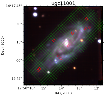
Figure 1: Colour composite RGB image recovered from MUSE data of one of the studied galaxies, UGC 11001. The red, green and blue images used to create RGB are obtained by integrating MUSE spectra in R, V and B filters, respectively. 500pc wide regions where spectra was extracted are overplotted as green and the regions identified as those on the envelope (defined above in section §4) are marked as red squares.

We use the MUSE (Bacon et al., 2010) reduced publicly available data for the galaxies listed in Table 1, from the ESO archive.

We first made a visual inspection to remove galaxies with no H$\alpha$ emission in the MUSE pointing, and thus to select MUSE fields where H$\alpha$ was observed, to be able to estimate recent star formation. After delimiting the regions with recent star formation, we divide each field into an integer number of observing squares, giving us squares with the closest (and larger than) size value to 500 pc. We show an example in Fig. 1, we do not use the squares outside the MUSE pointing. We choose 500 pc because it gives us a scale on which, from previous work, we expect to observe the self-regulation of star formation (Zaragoza-Cardiel et al., 2019), and it allows us to include galaxies at distances of up to 100 Mpc where 500 pc corresponds to 1 arcsec. We also need the foreground stars to be masked. We extract the spectrum for each defined region, correct it for Galactic extinction, and associate each with a redshift estimate, using the H$\alpha$ or [NII] at $6583.4\rm{\AA}$ if the later has a stronger peak than the former. We next estimate the [NII]/H$\alpha$ and the [OIII]/H$\beta$ flux ratios, and remove the regions which are classified as Seyfert-LINER in the BPT diagram (Kewley et al., 2006).

3 Stellar population synthesis and model fits

3.1 Stellar population synthesis

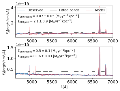
Figure 2: Two characteristic spectra for the galaxy NGC 716. Observed spectra are shown as blue lines. Top: the total star formation is dominated by the past star formation. Bottom: the total star formation is dominated by the recent star formation. The model spectrum which best fits the observed spectrum is shown as a red line. The continuum bands used to fit the observed spectrum to the combination of SSPs are shown as black lines.

We use SINOPSIS code (Fritz et al., 2007, 2017) to fit combinations of SSPs to the observed spectra. SINOPSIS fits equivalent widths of emission and absorption lines, as well as defined continuum bands. In this work, we use the H$\alpha$ and H$\beta$ equivalent widths, and the 9 continuum bands shown in Fig. 2, where we show two observed spectra of the galaxy NGC 716 and the resulted fits as an example.

We use the updated version of the Bruzual & Charlot models (Werle et al., 2019). We used SSPs of 3 metallicities ($Z=0.004$, $Z=0.02$, and $Z=0.04$) in 12 age bins (2 Myr, 4 Myr, 7 Myr, 20 Myr, 57 Myr, 200 Myr, 570 Myr, 1 Gyr, 3 Gyr, 5.75 Gyr, 10 Gyr, and 14 Gyr). We assume a free form of SFH, the Calzetti dust attenuation law (Calzetti et al., 2000), and the Chabrier 2003 IMF (Chabrier, 2003) for stellar masses between $0.1\rm{M_{\odot}}$ and $100\rm{M_{\odot}}$. The emission lines for the SSPs younger than 20 Myr are computed using the photoionisation code Cloudy (Ferland, 1993; Ferland et al., 1998; Ferland et al., 2013), assuming case B recombination (Osterbrock, 1989), an electron temperature of $10^{4}\rm{K}$, an electron density of $100\rm{cm}^{-3}$, and a gas cloud with an inner radius of $10^{-2}\rm{pc}$ (Fritz et al., 2017).

SINOPSIS uses the degeneracies between age, metallicity, and dust attenuation, to compute the uncertainties in the derived parameters (Fritz et al., 2007).

We rebin the different age bins into 4 bins: at $20\rm{Myr}$, $570\rm{Myr}$, $5.7\rm{Gyr}$, and $14\rm{Gyr}$. Simulated and observed spectra have been used to prove the validity of using SINOPSIS to recover these 4 age bins (Fritz et al., 2007, 2011). Additionally, SINOPSIS and similar codes have shown the reliability of recovering the SFH using synthesis of SSPs in, at least, 4 age bins (Cid Fernandes et al., 2005; Fritz et al., 2007, 2011; Sánchez et al., 2016). However, since we are interested in the recent star formation variations, we consider only the two most recent age bins, $20\rm{Myr}$, $570\rm{Myr}$, and call them recent, and past age bins, respectively. In this way we recover the recent, and the past star formation rate surface densities, $\Sigma_{\rm{SFR\thinspace recent}}$ and $\Sigma_{\rm{SFR\thinspace past}}$, which improves the confidence in the results presented in this work, since the two most recent age bins are better constrained than the oldest ones.

In order to use regions with a meaningful result, we take into account only regions with a signal to noise ratio (SNR) larger than 20 over the $[5350-5420]\thinspace\rm{\AA}$ range, and $\chi^{2}<3$. Due to IMF sampling effects, we also consider only regions where the recent SFR is larger than $10^{-3}\rm{M_{\odot}/yr}$ and the past SFR is larger than $10^{-5}\rm{M_{\odot}/yr}$.

Because we are limited to galaxies from Hubble Type Sa to Sdm, also excluding interacting galaxies and (U)LIRGs, the galaxy sample, by construction, is defined by galaxies that are probably on the star formation galaxy main sequence, and probably evolved via secular evolution in the studied age range (last 570 Myr), where by secular evolution we mean evolution dominated by slow processes (slower than many galaxy rotation periods Kormendy & Kennicutt (2004)). The galaxies probably evolved through more violent episodes in the past, but we are not affected by them in the studied age range. Nevertheless, individual zones such as the centres of the galaxies, might have evolved via rapid evolution due to high gas flows even in the studied age range. Because of this, we removed regions whose centres are at a distance of 500 pc or less from the centre of the galaxy, as well as regions having a very high recent SFR compared to the rest of the galaxy, specifically, we removed regions having $\Sigma_{\rm{SFR\thinspace recent}}$ larger than $\overline{\Sigma}_{\rm{SFR\thinspace recent}}+3\sigma_{\Sigma_{\rm{SFR\thinspace recent}}}$ for each galaxy. We will discuss how affects the results the removal of very high recent SFR regions in the discussion section (§6.4).

3.2 Fitting data to self-regulator the model

We have made the same assumptions made in Zaragoza-Cardiel et al. (2019) in order to fit our observables to the self-regulator model. For completeness, we briefly describe them here.

The self-regulator model (Eq. 2) is valid for a star or a group of co-rotating stars in the galaxy such as a massive star cluster (>500$\rm{M_{\odot}}$ Lada & Lada (2003)). Assuming $\eta$ constant, Eq. 2 is linear, so we can add up regions obeying that equation, and still obey the equation. In this context, the mass-loading factor would be representative of massive star clusters scales ($\sim$pc Lada & Lada (2003)). Although we find below that $\eta$ varies (Eq. 6), the variation is smooth enough to consider it approximately constant here. Therefore, the group of stars which are massive enough to produce bound clusters can be considered as a whole, while the less massive ones are splitted into individual stars. Feedback between different regions is then not considered here. We assume that our 500 pc wide regions are made of individual smaller regions obeying Eq 2, so we can rewrite Eq. 2 to be valid for our larger regions as the average of individual regions:

$$\dot{\overline{{\Sigma}}}_{\rm{gas}}=\dot{\overline{{\Sigma}}}_{\rm{net\thinspace flow}}-\overline{\Sigma}_{\rm{SFR}}(1-R+\eta).$$ (4)

We already showed in Zaragoza-Cardiel et al. (2019) that the resulted mass-loading factor was independent of the chosen scale (from 87pc to 1kpc) in NGC 628. Hence, regions can be added up while Eq. 4 is still valid.

The value of the $\overline{\Sigma}_{\rm{SFR\thinspace past}}$ we are able to measure is a time average over 550Myr. Since Eq. 4 is linear, we can substitute the time differentials by time average values over our age bin, and we will not be affected by possible bursts of the star formation, as long as the variation of $\eta$ is small enough (as we do find below).

The net gas flow rate surface density, $\dot{\overline{{\Sigma}}}_{\rm{net\thinspace flow}}$, is the change in gas density due to gas flows (independently of star formation), which can be negative, although in that case, the star formation is quenched (Zaragoza-Cardiel et al., 2019). This term, $\dot{\overline{{\Sigma}}}_{\rm{net\thinspace flow}}$, also includes the possibility of gas return from different regions and the same region at a later epoque, an effect known as galactic fountains (Fraternali, 2017). The observables are $\overline{\Sigma}_{\rm{SFR\thinspace recent}}$ and $\overline{\Sigma}_{\rm{SFR\thinspace past}}$. Let us assume that we can estimate $\dot{\overline{{\Sigma}}}_{\rm{gas}}$ from the star formation change considering the KS law, $\overline{\Sigma}_{\rm{SFR}}=A{\overline{{\Sigma}}}_{\rm{gas}}^{N}$, and rewrite Eq. 2:

$$\begin{split}&\overline{\Sigma}_{\rm{SFR\thinspace recent}}=\\ &A\left\{\left[\dot{\overline{\Sigma}}_{\rm{net\thinspace flow}}-\overline{\Sigma}_{\rm{SFR\thinspace past}}\left(1-R+\eta\right)\right]\Delta t+\left[\frac{\overline{\Sigma}_{\rm{SFR\thinspace past}}}{A}\right]^{\frac{1}{N}}\right\}^{N}.\end{split}$$ (5)

where there is a relation between our two observables ($\overline{\Sigma}_{\rm{SFR\thinspace recent}}$ and $\overline{\Sigma}_{\rm{SFR\thinspace past}}$), $\dot{\overline{{\Sigma}}}_{\rm{net\thinspace flow}}$, and $\eta$. We will use a simplistic approximation to estimate $\dot{\overline{{\Sigma}}}_{\rm{net\thinspace flow}}$, since we do not observe it. As explained in Zaragoza-Cardiel et al. (2019), we assume that several regions have an approximate value close to the maximum value of $\dot{\overline{{\Sigma}}}_{\rm{net\thinspace flow}}$, for a given galaxy. In the case of the estimation of $\eta$, although $\eta$ could vary between regions, we will find that the variation is smooth enough (Eq. 6) to consider the existence of a representative value for specific regions. In the following, for simplicity since we are only dealing with one type of regions, the 500 pc wide ones, we will be using the analysed terms (e.g. $\overline{\Sigma}_{\rm{SFR\thinspace recent}}$, $\overline{\Sigma}_{\rm{SFR\thinspace past}}$, $\dot{\overline{{\Sigma}}}_{\rm{net\thinspace flow}}$) without the need of using the average symbols ($\Sigma_{\rm{SFR\thinspace recent}}$, $\Sigma_{\rm{SFR\thinspace past}}$, $\dot{{\Sigma}}_{\rm{net\thinspace flow}}$). Therefore, when we present an average, the average will be for several 500pc wide regions.

Assuming the instantaneous recycling approximation (Madau & Dickinson, 2014) for stars more massive than $3\rm{M_{\odot}}$ ($\tau_{\rm{MS}}\sim 0.6\rm{Gyr}$, where $\tau_{\rm{MS}}$ is the main sequence lifetime), and a Chabrier IMF (Chabrier, 2003), we obtain a value of $R=0.27$. We use the values $A=10^{-4.32}\rm{M_{\odot}/kpc^{2}/yr}$, and $N=1.56$ for the KS lawKennicutt et al. (2007).

4 Results

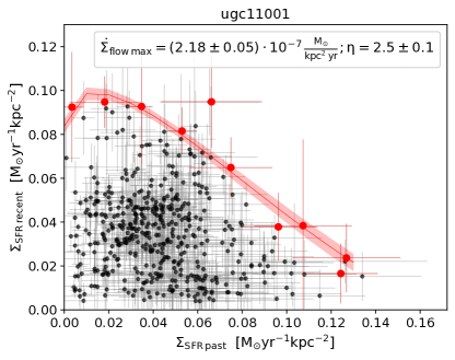
Figure 3: Recent star formation rate surface density, $\Sigma_{\rm{SFR\thinspace recent}}$, versus the past star formation rate surface density, $\Sigma_{\rm{SFR\thinspace past}}$, for the UGC 11001 galaxy. The red dots are the regions identified as those on the envelope. We plot the fit of Eq. 5 to the regions on the envelope as well as the result of the fit and the 1-$\sigma$ uncertainty range of the fit as shaded region.

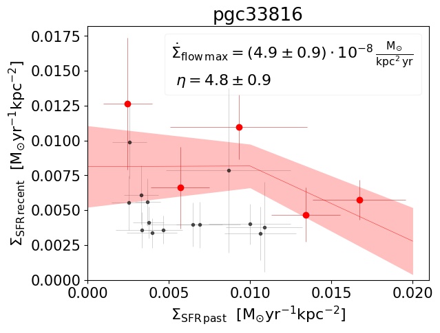
(a)

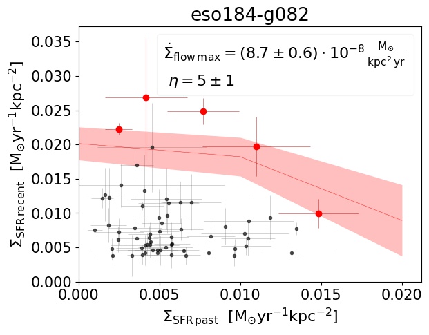
(b)

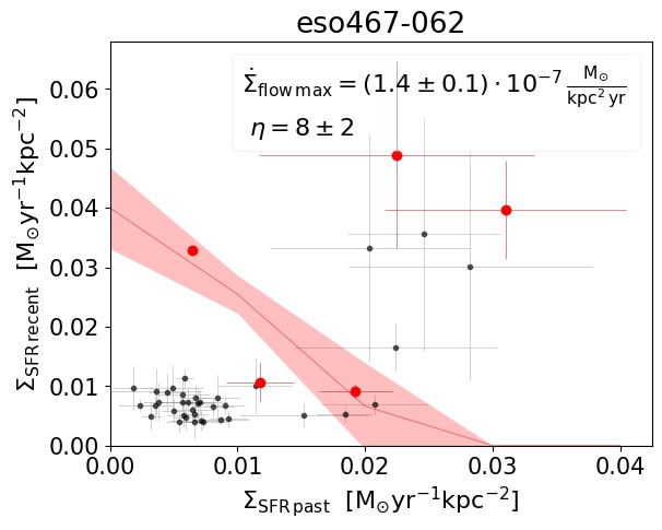
(c)

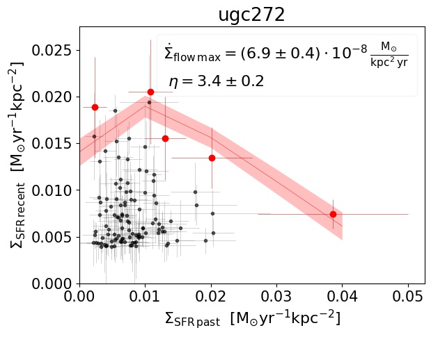
(d)

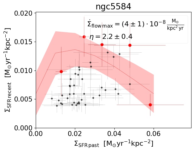
(e)

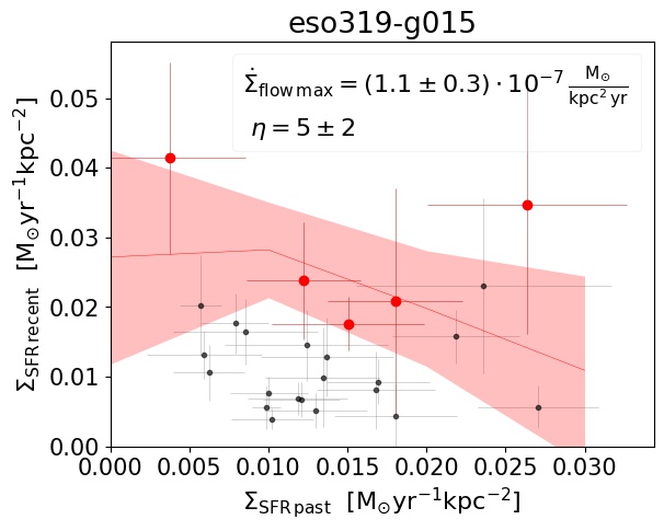
(f)

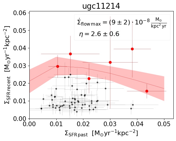
(g)

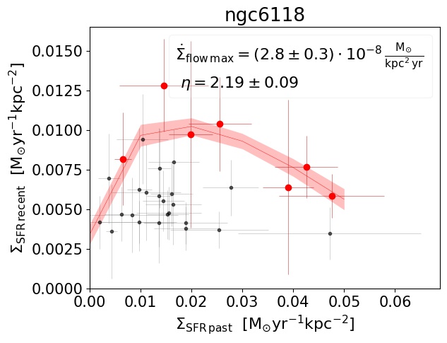
(h)

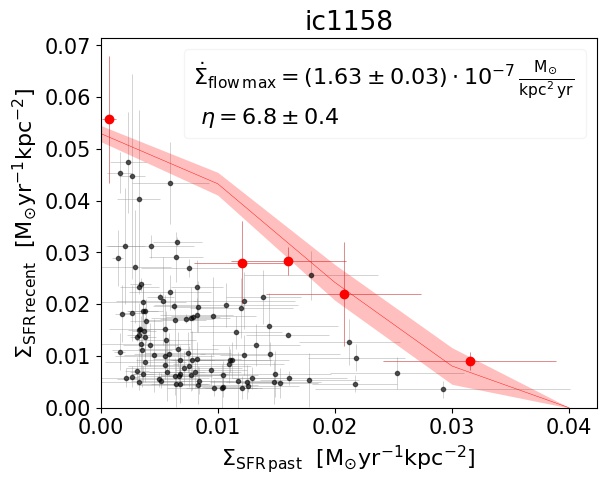
(i)

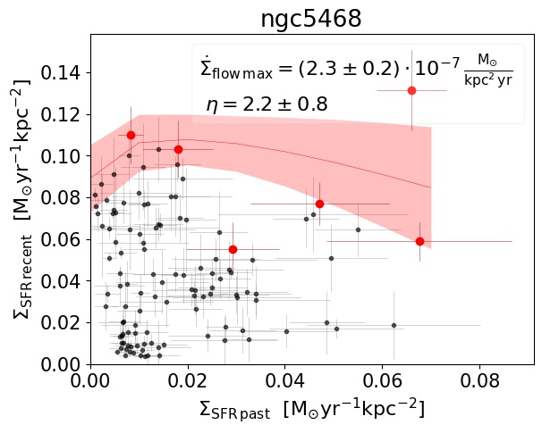
(j)

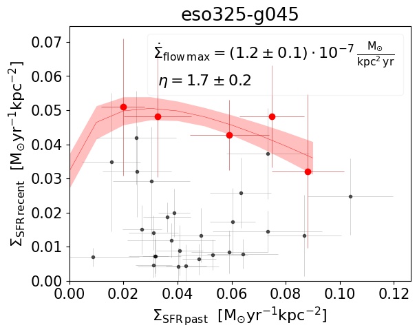
(k)

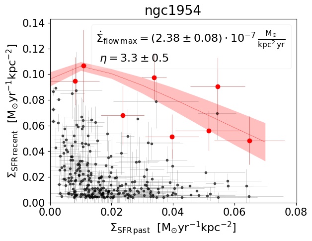
(l)

Figure 8: SFR recent-past diagrams. Recent star formation surface density, $\Sigma_{\rm{SFR\thinspace recent}}$, versus the past star formation rate surface density, $\Sigma_{\rm{SFR\thinspace past}}$, for each galaxy of the sample. The red dots are the regions identified as those on the envelope. We plot the fit of Eq. 5 to the regions on the envelope and the 1-$\sigma$ uncertainty range of the fit as shadow region. We show the parameters of the fit, at the top of each panel.

As an example, we plot the $\Sigma_{\rm{SFR\thinspace recent}}$ versus $\Sigma_{\rm{SFR\thinspace past}}$ diagram for one of the galaxies, UGC 11001, in Fig. 3. We plot the $\Sigma_{\rm{SFR\thinspace recent}}$ versus $\Sigma_{\rm{SFR\thinspace past}}$ diagrams for all of the galaxies in Fig. 8. Each of the points in these plots can be seen as the relation between the $\Sigma_{\rm{SFR\thinspace recent}}$ and the $\Sigma_{\rm{SFR\thinspace past}}$ which depends on the value of $\dot{\Sigma}_{\rm{net\thinspace flow}}$, and $\eta$ (Eq. 5).

We identify those regions having the maximum $\Sigma_{\rm{SFR\thinspace recent}}$, per bin of $\Sigma_{\rm{SFR\thinspace past}}$, as the regions on the envelope. We see the regions on the envelope as red dots in Fig. 3, and as red squares in the MUSE recovered false color image of UGC 11001 in Fig. 1.

Table 3: Estimated mass-loading factors, $\eta$, maximum flow gas surface density term, $\dot{\Sigma}_{\rm{flow\thinspace max}}$, and the associated average stellar mass surface density for the regions on the envelope, $\Sigma_{*}$.

Galaxy identifier	$\eta$ a	$\dot{\Sigma}_{\rm{flow\thinspace max}}$ b	$\Sigma_{*}$ c
		$10^{-8}\rm{M_{\odot}\thinspace yr^{-1}\thinspace kpc^{-2}}$	$10^{6}\rm{M_{\odot}\thinspace kpc^{-2}}$
pgc33816	$4.8\pm 0.9$	$4.9\pm 0.9$	$27\pm 15$
eso184-g082	$5.0\pm 1.0$	$8.7\pm 0.6$	$49\pm 20$
eso467-062	$8.0\pm 2.0$	$14.0\pm 1.0$	$51\pm 39$
ugc272	$3.4\pm 0.2$	$6.9\pm 0.4$	$57\pm 44$
ngc5584	$2.2\pm 0.4$	$4.0\pm 1.0$	$60\pm 31$
eso319-g015	$5.0\pm 2.0$	$11.0\pm 3.0$	$66\pm 65$
ugc11214	$2.6\pm 0.6$	$9.0\pm 2.0$	$84\pm 33$
ngc6118	$2.19\pm 0.09$	$2.8\pm 0.3$	$90\pm 51$
ic1158	$6.8\pm 0.4$	$16.3\pm 0.3$	$109\pm 28$
ngc5468	$2.2\pm 0.8$	$23.0\pm 2.0$	$113\pm 66$
eso325-g045	$1.7\pm 0.2$	$12.0\pm 1.0$	$121\pm 57$
ngc1954	$3.3\pm 0.5$	$23.8\pm 0.8$	$121\pm 31$
ic5332	$3.0\pm 1.0$	$12.0\pm 2.0$	$120\pm 100$
ugc04729	$2.8\pm 0.6$	$7.0\pm 2.0$	$126\pm 57$
ngc2104	$1.7\pm 0.6$	$4.0\pm 2.0$	$132\pm 62$
eso316-g7	$2.0\pm 1.0$	$12.0\pm 6.0$	$136\pm 39$
eso298-g28	$6.0\pm 0.7$	$47.0\pm 2.0$	$136\pm 46$
mcg-01-57-021	$7.0\pm 1.0$	$17.0\pm 2.0$	$137\pm 24$
pgc128348	$2.9\pm 0.1$	$11.6\pm 0.7$	$140\pm 92$
pgc1167400	$2.3\pm 0.3$	$4.1\pm 0.8$	$141\pm 78$
ngc2835	$2.2\pm 0.7$	$7.0\pm 3.0$	$144\pm 40$
ic2151	$2.0\pm 0.5$	$5.0\pm 3.0$	$146\pm 61$
ngc988	$1.2\pm 0.4$	$1.0\pm 2.0$	$158\pm 63$
ngc1483	$3.0\pm 2.0$	$13.0\pm 5.0$	$158\pm 40$
ngc7421	$1.1\pm 0.3$	$1.0\pm 0.9$	$167\pm 78$
fcc290	$2.0\pm 0.4$	$3.0\pm 1.0$	$169\pm 42$
ic344	$2.5\pm 0.2$	$11.0\pm 1.0$	$171\pm 78$
ngc3389	$4.4\pm 0.7$	$32.4\pm 0.7$	$190\pm 130$
eso246-g21	$2.9\pm 0.7$	$7.0\pm 2.0$	$188\pm 67$
pgc170248	$4.9\pm 0.7$	$16.0\pm 1.0$	$192\pm 77$
ngc7329	$4.1\pm 0.2$	$7.8\pm 0.4$	$200\pm 120$
ugc12859	$2.8\pm 0.3$	$5.1\pm 0.9$	$202\pm 90$
ugc1395	$2.7\pm 0.3$	$8.0\pm 1.0$	$200\pm 160$
ngc5339	$2.9\pm 0.4$	$5.0\pm 1.0$	$210\pm 150$
ngc1591	$2.3\pm 0.7$	$19.0\pm 4.0$	$212\pm 93$
pgc98793	$1.7\pm 0.1$	$6.6\pm 0.8$	$214\pm 95$
ugc5378	$2.7\pm 0.4$	$10.0\pm 1.0$	$223\pm 93$
ngc4806	$1.9\pm 0.2$	$10.3\pm 0.9$	$230\pm 170$
ngc1087	$1.3\pm 0.3$	$14.0\pm 2.0$	$230\pm 170$
ngc4980	$1.8\pm 0.3$	$6.6\pm 0.9$	$240\pm 170$
ngc6902	$2.4\pm 0.3$	$8.0\pm 1.0$	$240\pm 13$
ugc11001	$2.5\pm 0.1$	$21.8\pm 0.5$	$250\pm 140$
ic217	$1.2\pm 0.4$	$3.0\pm 2.0$	$266\pm 88$
eso506-g004	$3.4\pm 0.2$	$13.9\pm 0.4$	$270\pm 170$
ic2160	$2.4\pm 0.4$	$12.0\pm 2.0$	$270\pm 260$
ngc1385	$0.9\pm 0.1$	$9.7\pm 0.9$	$272\pm 44$
mcg-01-33-034	$1.0\pm 0.09$	$7.9\pm 0.5$	$270\pm 150$
ngc4603	$0.9\pm 0.1$	$3.0\pm 1.0$	$276\pm 85$
ngc4535	$4.1\pm 0.7$	$15.0\pm 2.0$	$280\pm 200$
ngc1762	$2.3\pm 0.2$	$8.2\pm 0.7$	$290\pm 140$
ngc3451	$3.7\pm 0.4$	$11.0\pm 1.0$	$300\pm 180$
ngc4790	$1.2\pm 0.3$	$9.0\pm 2.0$	$334\pm 63$
ngc3244	$1.8\pm 0.2$	$8.0\pm 1.0$	$340\pm 270$
ngc628	$1.8\pm 0.1$	$19.0\pm 1.0$	$360\pm 170$
pgc30591	$0.7\pm 0.4$	$0.0\pm 2.0$	$360\pm 160$
ngc5643	$1.1\pm 0.3$	$3.0\pm 2.0$	$410\pm 160$
ngc1309	$1.3\pm 0.2$	$17.0\pm 2.0$	$420\pm 220$

^a Mass-loading factor derived in this work. ^b Maximum flow gas surface density term derived in this work. ^c Stellar mass surface density for the regions on the envelope obtained in this work.

Table 4: continued

Galaxy identifier	$\eta$ a	$\dot{\Sigma}_{\rm{flow\thinspace max}}$ b	$\Sigma_{*}$ c
		$10^{-8}\rm{M_{\odot}\thinspace yr^{-1}\thinspace kpc^{-2}}$	$10^{6}\rm{M_{\odot}\thinspace kpc^{-2}}$
ngc1084	$0.6\pm 0.2$	$13.0\pm 6.0$	$420\pm 170$
ngc7580	$1.6\pm 0.2$	$18.0\pm 1.0$	$420\pm 110$
ngc692	$2.7\pm 0.2$	$14.0\pm 1.0$	$420\pm 220$
eso462-g009	$4.0\pm 1.0$	$8.0\pm 2.0$	$440\pm 310$
ic5273	$1.5\pm 0.7$	$9.0\pm 4.0$	$450\pm 220$
pgc3140	$1.0\pm 0.1$	$4.0\pm 1.0$	$460\pm 210$
ic1553	$0.6\pm 0.3$	$5.0\pm 2.0$	$460\pm 290$
ugc11289	$1.8\pm 0.3$	$8.0\pm 3.0$	$472\pm 46$
ic4582	$2.0\pm 0.1$	$9.1\pm 0.5$	$480\pm 280$
ngc2466	$1.5\pm 0.2$	$18.0\pm 2.0$	$480\pm 470$
eso443-21	$1.9\pm 0.3$	$94.0\pm 4.0$	$490\pm 180$
ic4452	$0.37\pm 0.05$	$5.2\pm 0.6$	$500\pm 320$
eso498-g5	$1.5\pm 0.3$	$20.0\pm 2.0$	$510\pm 320$
eso552-g40	$1.7\pm 0.4$	$12.0\pm 3.0$	$540\pm 280$
eso163-g11	$0.48\pm 0.06$	$1.0\pm 2.0$	$570\pm 300$
ngc7582	$0.6\pm 0.1$	$0.0\pm 2.0$	$570\pm 280$
ngc1620	$1.4\pm 0.3$	$8.0\pm 2.0$	$580\pm 400$
ic1320	$1.4\pm 0.1$	$4.6\pm 0.9$	$590\pm 270$
ngc3393	$1.9\pm 0.3$	$11.0\pm 1.0$	$590\pm 270$
ngc2370	$0.87\pm 0.08$	$4.0\pm 2.0$	$600\pm 310$
ngc4981	$0.85\pm 0.08$	$7.0\pm 1.0$	$630\pm 580$
ngc3783	$1.3\pm 0.3$	$12.0\pm 3.0$	$680\pm 170$
ngc1285	$0.8\pm 0.1$	$7.0\pm 2.0$	$700\pm 460$
ngc5806	$1.7\pm 0.3$	$17.0\pm 3.0$	$720\pm 530$
eso018-g018	$1.0\pm 0.3$	$13.0\pm 5.0$	$720\pm 420$
ngc6754	$0.44\pm 0.06$	$1.0\pm 1.0$	$750\pm 480$
ic2560	$1.2\pm 0.2$	$11.0\pm 1.0$	$760\pm 370$
ngc7140	$2.4\pm 0.7$	$13.0\pm 6.0$	$770\pm 210$
ngc3464	$1.9\pm 0.3$	$9.0\pm 3.0$	$780\pm 380$
mcg-02-13-38	$1.3\pm 0.1$	$20.0\pm 1.0$	$790\pm 450$
ngc1590	$0.83\pm 0.08$	$25.0\pm 3.0$	$810\pm 460$
pgc8822	$1.15\pm 0.09$	$4.0\pm 1.0$	$970\pm 430$
ngc7721	$1.3\pm 0.5$	$10\pm 10$	$990\pm 540$
pgc28308	$0.2\pm 0.1$	$0.0\pm 8.0$	$1030\pm 450$
ngc1137	$0.8\pm 0.2$	$1.0\pm 4.0$	$1030\pm 830$
eso478-g006	$1.1\pm 0.2$	$10.0\pm 4.0$	$1050\pm 650$
ngc1448	$1.05\pm 0.09$	$15.0\pm 2.0$	$1130\pm 480$
ngc3278	$1.3\pm 0.2$	$31.0\pm 3.0$	$1170\pm 710$
ngc4030	$0.6\pm 0.1$	$14.0\pm 3.0$	$1310\pm 550$
ngc3363	$0.41\pm 0.08$	$0.0\pm 0.9$	$1330\pm 590$
ngc7780	$1.2\pm 0.2$	$8.0\pm 3.0$	$1450\pm 590$
ic1438	$1.5\pm 0.3$	$11.0\pm 4.0$	$1520\pm 250$
ngc4666	$0.3\pm 0.1$	$10.0\pm 3.0$	$2900\pm 1300$
ngc7396	$0.5\pm 0.2$	$0.0\pm 4.0$	$4100\pm 1900$
ngc716	$0.5\pm 0.2$	$70\pm 10$	$5200\pm 1900$

We can see in Eq. 5 that we need the value of $\dot{\Sigma}_{\rm{net\thinspace flow}}$ in combination with the $\Sigma_{\rm{SFR\thinspace recent}}$ and $\Sigma_{\rm{SFR\thinspace past}}$ values, in order to quantify $\eta$. For a given galaxy, there should be a maximum value for the net flow gas surface density term, $\dot{\Sigma}_{\rm{flow\thinspace max}}$. Although in principle $\dot{\Sigma}_{\rm{flow\thinspace max}}$ is unknown for us, if we assume that there are several segments where $\dot{\Sigma}_{\rm{net\thinspace flow}}\sim\dot{\Sigma}_{\rm{flow\thinspace max}}$, then these regions are those on the $\Sigma_{\rm{SFR\thinspace recent}}$ versus $\Sigma_{\rm{SFR\thinspace past}}$ diagram envelope.

Assuming $\dot{\Sigma}_{\rm{net\thinspace flow}}$ constant, we fit Eq. 5 to the regions on the envelope and estimate the mass-loading factor, representative of those specific regions. We have selected a galaxy sample mainly composed by galaxies on the main sequence of star formation, and remove segments having very high $\Sigma_{\rm{SFR\thinspace recent}}$ compared to the rest of the segments of a galaxy. Therefore, the galaxy sample, as well as the segments, have been chosen to assure the $\dot{\Sigma}_{\rm{net\thinspace flow}}\sim\dot{\Sigma}_{\rm{flow\thinspace max}}$ hypothesis for several regions. The regions below the envelope are due, to a greater extent, to regions having a smaller value of $\dot{\Sigma}_{\rm{net\thinspace flow}}<\dot{\Sigma}_{\rm{flow\thinspace max}}$, and to a much lesser extent, to regions having different $\eta$ values.

We have fitted Eq. 5 to the envelopes of the 102 galaxy listed in Table 1 and show the results in Fig. 3 for UGC 11001, and in Fig. 8 for the rest of the galaxies, as a red line.

4.1 Variations of $\eta$

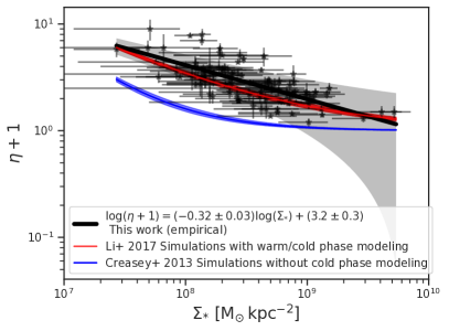
Figure 4: Local mass-loading factor, $\eta$, versus the average stellar mass surface density of the regions on the envelope for each galaxy, $\Sigma_{*}$, as black stars. We plot the linear fit to the empirically derived quantities and the 1-$\sigma$ uncertainty range of the fit as shaded regions. The blue line shows the $\eta$ reported for supernova explosions hydrodynamical simulations (Creasey et al., 2013) with cut-off cooling modeling, and as blue line the $\eta$ reported for supernova explosions hydrodynamical simulations (Li et al., 2017) with gas cold-phase modeling included.

Although we have an $\eta$ value for each galaxy, $\eta$ is an average value representative only of the regions on the envelope, instead of the whole galaxy. We associate the estimated $\eta$ for a given envelope with the average surface stellar mass density, $\Sigma_{*}$, of those regions on the envelope where we estimate $\eta$. Therefore, $\eta$ is a local average value, representative only of the regions on the envelope, and their mean value of $\Sigma_{*}$. Although $\eta$ value might vary through the regions on the envelope, we assume that the variation is smooth enough and associate the average stellar mass density, $\Sigma_{*}$ and the standard deviation, to each envelope. The correlation found between $\eta$ and $\Sigma_{*}$ (Eq. 6 and Fig. 4) is in fact smooth enough to make the association between $\eta$ and $\Sigma_{*}$ for the regions on the envelope. We report $\eta$, $\dot{\Sigma}_{\rm{flow\thinspace max}}$, and $\Sigma_{*}$ values in Table 3.

We plot in Fig. 4, $\eta$ versus $\Sigma_{*}$, and find that the mass-loading factors strongly correlate with the local $\Sigma_{*}$ measured on the envelope regions:

$$\log(\eta+1)=(-0.32\pm 0.03)\log(\Sigma_{*})+(3.2\pm 0.3)$$ (6)

This correlation means that the denser the region, the lower is the mass-loading factor, which means that the amount of outflowing gas mass per unit star formation rate depends inversely on the stellar mass surface density. This is so because the denser the region, the larger is the local gravitational pull, making it harder for the gas to be expelled. The local chemical enrichment of galaxies (Barrera-Ballesteros et al., 2018) also favours the gas regulator model and finds that the mass-loading factor depends on the local escape velocity. This new empirical $\eta$-$\Sigma_{*}$ relation, can be used to check if stellar feedback implementations in numerical simulations (Hopkins et al., 2014; Li et al., 2017; Creasey et al., 2013) are realistic. In particular, we can compare our $\eta$-$\Sigma_{*}$ relation with the $\eta$-$\Sigma_{\rm{gas}}$ relation from supernova explosion feedback simulations (Li et al., 2017; Creasey et al., 2013), using the observed $\Sigma_{*}$-$\Sigma_{\rm{gas}}$ relation (Barrera-Ballesteros et al., 2020). The inverse correlation between $\eta$ and $\Sigma_{*}$ is clear from observations and simulations. However, our empirical result supports that the radiative cooling below $10^{4}\rm{K}$ is important. This is because when ignoring gas cooling below $10^{4}\rm{K}$, there is an excess of warm gas compared with the models including a multiphase cold/warm gas (Li et al., 2017). Thus, in the warm gas excess scenario, there is a layer of gas with higher ISM pressure which prevents the gas to be expelled from the supernova explosions.

5 Local to global mass-loading factors

The mass-loading factor derived here is representative of local scales. However, other observational and theoretical studies report global mass-loading factors (Muratov et al., 2015; Rodríguez-Puebla et al., 2016; Hayward & Hopkins, 2017; Schroetter et al., 2019; McQuinn et al., 2019). We estimate global mass-loading factors, $\eta_{\rm{G}}$, from the empirical $\eta$-$\Sigma_{*}$ relation reported here (Eq. 6), integrating over observed stellar mass density profiles.

To convert $\eta$ to $\eta_{\rm{G}}$, we assume that we can estimate the total outflow due to stellar feedback, $\dot{M}_{\rm{out}}$, by adding up $\dot{\Sigma}_{\rm{out}}$ over each individual segment where stellar feedback acts. Since we are interested in galaxy discs, we assume a radial characterization for the properties of interest, i.e., $\eta$, $\dot{\Sigma}_{\rm{out}}$, $\Sigma_{\rm{SFR}}$, and $\Sigma_{\rm{SFR}}$ depend on $R$, the radial distance to the centre of the disc:

$$\eta_{\rm{G}}=\frac{\dot{M}_{\rm{out}}}{\rm{SFR}}=\frac{\int_{0}^{\infty}\dot{\Sigma}_{\rm{out}}(R)R\thinspace{\rm{d}}R}{\int_{0}^{\infty}\Sigma_{\rm{SFR}}(R)R\thinspace{\rm{d}}R}=\frac{\int_{0}^{\infty}\eta(R)\Sigma_{\rm{SFR}}(R)R\thinspace{\rm{d}}R}{\int_{0}^{\infty}\Sigma_{\rm{SFR}}(R)R\thinspace{\rm{d}}R}.$$ (7)

The conversion between $\eta$ to $\eta_{\rm{G}}$ is a $\Sigma_{\rm{SFR}}$ weighted average of $\eta$. Stellar mass density profiles, $\Sigma_{*}(R)$, are better constrained than $\Sigma_{\rm{SFR}}(R)$ profiles, so we decide to use the empirical relation between $\Sigma_{\rm{SFR}}\propto\Sigma_{*}(R)^{n}$. For simplicity, we assume $n=1$, which is consistent with the latest results of this relation for galaxy discs (Cano-Díaz et al., 2019), although we found that different $n$ values close to 1 do not change the results significantly. Using our empirical relation (Eq. 6) we rewrite Eq. 7:

$$\eta_{\rm{G}}=\frac{\int_{0}^{\infty}\eta(R)\Sigma_{*}(R)R\thinspace{\rm{d}}R}{\int_{0}^{\infty}\Sigma_{*}(R)R\thinspace{\rm{d}}R}=\frac{10^{3.2}\int_{0}^{\infty}{\Sigma_{*}(R)}^{0.68}R\thinspace{\rm{d}}R}{\int_{0}^{\infty}\Sigma_{*}(R)R\thinspace{\rm{d}}R}.$$ (8)

The stellar mass surface density profile, $\Sigma_{*}(R)$, is therefore all we need to compute the global mass-loading factor. We use the deepest stellar mass surface density profiles from the Spitzer Survey of Stellar Structure in Galaxies (S4G) (Díaz-García et al., 2016) to compute the global mass-loading factor as a function of stellar mass. S4G stellar mass surface density profiles are divided into 5 mass bins: $[10^{8.5}$-$10^{9}]$, $[10^{9}$-$10^{9.5}]$, $[10^{9.5}$-$10^{10}]$, $[10^{10}$-$10^{10.5}]$, and $[10^{10.5}$-$10^{11}]\thinspace\rm{M_{\odot}}$. We used these 5 mass bins to compute the $\eta_{\rm{G}}$ shown in Fig. 5.

5.1 Variations of $\eta_{\rm{G}}$

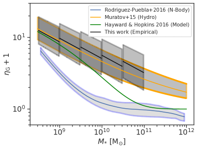
Figure 5: Global mass-loading factor, $\eta_{\rm{G}}$, versus the stellar mass of the galaxy, $M_{*}$. The black lines show the empirical quantities which have been derived combining the distribution of $\eta$ as a function of stellar mass surface density (Fig. 4) with the stellar mass surface density profiles from S4G results (Díaz-García et al., 2016), where the shaded region is the corresponding uncertainty propagated from the 1-$\sigma$ uncertainty found in the $\eta$-$\Sigma_{*}$ relation (Eq. 6). The discontinuity is due to the division in different parametrizations of the stellar mass surface density profiles in 5 mass bins reported by Díaz-García et al. (2016). The orange line shows the $\eta_{\rm{G}}$ reported for cosmological zoom-in galaxy hydrodynamical simulations (Muratov et al., 2015), the green line the shows an analytical feedback model (Hayward & Hopkins, 2017), and the blue line shows the $\eta_{\rm{G}}$ reported using the N-body Bolshoi-Planck simulation (Rodríguez-Puebla et al., 2016).

We present our empirically derived global mass-loading factors as a function of stellar mass in Fig. 5 as black lines. The discontinuity is due to the division in different parametrizations of the stellar mass surface density profiles in 5 mass bins reported by Díaz-García et al. (2016) . The most important feature we find in Fig. 5 is that the smaller the stellar mass of the galaxy, the larger the mass-loading factor, as required to reconcile the ratio of halo to stellar mass in low-mass galaxies (Behroozi et al., 2010; Rodríguez-Puebla et al., 2016). We compare our empirical estimates with predictions based on N-body (Rodríguez-Puebla et al., 2016) and hydrodynamical simulations (Muratov et al., 2015), as well as with an analytical model (Hayward & Hopkins, 2017).

Some simulations, as well as the analytic model we used to compare with, define the mass-loading factor using the outflowing mass that escapes the galaxy forever (Rodríguez-Puebla et al., 2016; Hayward & Hopkins, 2017). Therefore, they do not consider the outflowing gas which returns to the galaxy at a later time which, depending on the outflow velocity, will result in smaller mass-loading factors. We define the mass-loading factor as the total mass ejected independently of velocity, and the mass can come back at a later time (outside the 550Myr time range). There is a remarkable agreement between our empirical result and that from hydrodynamical simulations that define the mass-loading factor as independent of velocity (Muratov et al., 2015). In fact, for lower masses ($M_{*}<10^{9.5}\rm{M_{\odot}}$), where the stellar feedback is thought to be more important regulating galaxy stellar mass growth, and the escape velocity lower, the agreement with the analytic model is also remarkably good.

6 Discussion

6.1 Comparison with other studies

The results reported here are slightly different when we compare them with recent observational studies reporting local (Kruijssen et al., 2019; Roberts-Borsani et al., 2020) and global (Schroetter et al., 2019; McQuinn et al., 2019) mass-loading factors.

The reported local mass-loading factors using the spatial de-correlation between star formation and molecular gas (Kruijssen et al., 2019) differ by less than $3\sigma$ from our reported values, and it might be due to the smaller time scale of $\sim 1.5\rm{Myr}$ for which they report efficient gas dispersal, while our reported time scale is $\sim 550\rm{Myr}$. The previously reported local mass-loading factors using the Na D absorption (Roberts-Borsani et al., 2020) are consistent with ours within $1\sigma$.

The use of Mg II absorption of the circum-galactic medium to derive global mass-loading factors gives no clear dependence on the total mass of the galaxy (Schroetter et al., 2019). However, the Mg II absorption method gives $\eta_{\rm{G}}$ with very high uncertainties, mainly due to the uncertainty when deriving the HI column density from the Mg II equivalent width (Schroetter et al., 2015). Due to these large uncertainties, their results are apparently consistent with our results within 1$\sigma$ for most of their reported $\eta_{\rm{G}}$’s.

The mass-loading factor estimates using deep H$\alpha$ imaging give smaller mass-loading factors compared to those reported here and give no correlation with the stellar mass of the galaxy (McQuinn et al., 2019). Nevertheless, the method using H$\alpha$ imaging derives the amount of outflowing gas from the H$\alpha$ surface brightness background, so it neglects H$\alpha$ emission stronger than this background emission. The estimated outflowing mass could be inferior to the real one since we already know that H$\alpha$ emission has a component due to expansive bubbles (Relaño & Beckman, 2005; Camps-Fariña et al., 2015).

6.2 Discussion on envelope’s shapes

Eq. 5 depends on $\dot{\Sigma}_{\rm{flow\thinspace max}}$, $\eta$, $\Sigma_{\rm{SFR\thinspace recent}}$, and $\Sigma_{\rm{SFR\thinspace past}}$ values. The case shown in Fig. 3, where there is no high recent star formation rate for those regions where the past star formation rate was the highest, is a common case, but not the only one. For instance, there are cases where $\Sigma_{\rm{SFR\thinspace recent}}$ values are approximately constant through the regions on the envelope or even increase as $\Sigma_{\rm{SFR\thinspace past}}$ increase (e.g. NGC 988, NGC 7421, IC 217, IC 4452, PGC 28308 in Fig. 8).

Essentially, there are two terms depending on $\Sigma_{\rm{SFR\thinspace past}}$ in Eq. 5, one with a direct proportionality and the other with an inverse one. The latter dominates for larger $\eta$ values meaning that the larger the mass-loading factor, the larger is the effect in reducing the amount of gas to form stars, as expected. However, for small enough $\eta$ and $\Sigma_{\rm{SFR\thinspace past}}$ values, the directly dependent term can dominate producing a direct relation between $\Sigma_{\rm{SFR\thinspace recent}}$ and $\Sigma_{\rm{SFR\thinspace past}}$, as we see in some galaxies in Fig. 8 (e.g. IC 4452). The extrapolation of Eq. 5 to large enough values of $\Sigma_{\rm{SFR\thinspace past}}$ would give always a decrease in $\Sigma_{\rm{SFR\thinspace recent}}$, as long as $\eta>0$, and that is the reason to observe some inverted U-shape envelopes (e.g. NGC 1084, PGC 3140).

Finally, for large enough $\dot{\Sigma}_{\rm{flow\thinspace max}}$ values, the directly $\Sigma_{\rm{SFR\thinspace past}}$ dependent term is almost negligible for small values of $\Sigma_{\rm{SFR\thinspace past}}$, and then the recent star formation depends on $\dot{\Sigma}_{\rm{flow\thinspace max}}$ for the low $\Sigma_{\rm{SFR\thinspace past}}$, while decreases proportionally with $\Sigma_{\rm{SFR\thinspace past}}$ depending on the mass-loading factor (e.g UGC 5378, UGC 11001).

Therefore, the combination of $\dot{\Sigma}_{\rm{flow\thinspace max}}$ and $\eta$ variations, as well as the range covered by the past and recent star formation rate surface densities, is what gives the different envelope’s shapes. The uncertainties obtained when fitting Eq. 5 show reliable estimates, except for one case, the PGC 30591 galaxy, which is the one having the highest inclination of our sample.

6.3 High-inclination galaxies

Although we have removed edge-on ($i=90^{\circ}$) galaxies from our sample, high-inclination ($i>70^{\circ}$) galaxies might not be good candidates to apply the method used in this study, as in the case of the PGC 30591 galaxy. In the case of edge-on and very high-inclination galaxies, two main effects can affect the pertinence of applying the method. Firstly, one can have in the line of sight a large combination of different regions of the galaxy. Secondly, the higher the inclination, the smaller is the number of resolved regions, while the method relies on a large enough number of resolved regions.

Nevertheless, except for PGC 30591, we found reliable $\dot{\Sigma}_{\rm{flow\thinspace max}}$ and $\eta$ estimates, even for high-inclination galaxies. Including or excluding high-inclination galaxies does not make any changes to the reported $\eta$-$\Sigma_{*}$ relation presented here. We show in Fig. 6 the $\eta$-$\Sigma_{*}$ observed and fitted relations for high-inclination galaxies, as star symbols and black line, respectively. When we compare the high-inclination galaxies results with the fit obtained using the full sample (Eq. 6), shown as a red line, both samples are compatible within $1\sigma$.

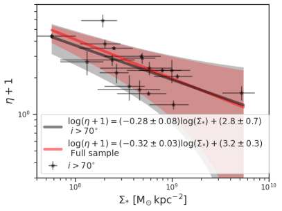
Figure 6: Local mass-loading factor, $\eta$, versus the average stellar mass surface density of the regions on the envelope for each galaxy, $\Sigma_{*}$, as black stars, for high-inclination galaxies. We plot, as a black line, the linear fit to the empirically derived quantities. We plot as a red line, the fit for the full sample (Eq. 6), and the 1-$\sigma$ uncertainty range of the fits as shaded regions.

6.4 Effects of very high recent SFR regions removal

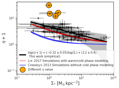
Figure 7: Local mass-loading factor, $\eta$, versus the average stellar mass surface density of the regions on the envelope for each galaxy, $\Sigma_{*}$, as black stars. Same plot as in Fig. 4, but this version of the plot has been done without removing any region based on its $\Sigma_{\rm{SFR\thinspace recent}}$ value. The 4 galaxies where we find a significant difference in the derived $\eta$ value are marked as orange circles. We plot the linear fit to the empirically derived quantities and the 1-$\sigma$ uncertainty range of the fit as shaded regions. The blue line shows the $\eta$ reported for supernova explosions hydrodynamical simulations (Creasey et al., 2013) with cut-off cooling modeling, and as blue line the $\eta$ reported for supernova explosions hydrodynamical simulations (Li et al., 2017) with gas cold-phase modeling included.

We think is important to remove regions having very high values of $\Sigma_{\rm{SFR\thinspace recent}}$ compared to the rest of the galaxy, since these regions probably have a very high $\dot{\Sigma}_{\rm{net\thinspace flow}}$ value compared to the rest of the regions identified to be on the envelope. The effect of considering these high $\Sigma_{\rm{SFR\thinspace recent}}$ regions affects our assumption about the approximate equal value of $\dot{\Sigma}_{\rm{net\thinspace flow}}$ for the regions on the envelope.

However, in order to explore the effect of this removal in our results, we have performed the same analysis without removing any region based on its $\Sigma_{\rm{SFR\thinspace recent}}$ value. We plot the derived $\eta$ versus the local $\Sigma_{*}$ of the regions on the envelope for the whole sample of galaxies in Fig. 7. We also plot the resulted $\eta$-$\Sigma_{*}$ fit to the observed data. We find a very similar correlation between $\eta$ and the local $\Sigma_{*}$:

$$\log(\eta+1)=(-0.32\pm 0.05)\log(\Sigma_{*})+(3.2\pm 0.4).$$ (9)

There are only 4 galaxies where the $\eta$ value significantly changes: IC 1158, NGC 3389, ESO 298-G28, and MCG 01-57-021. We marked these galaxies as orange circles in Fig. 7. However, the changes are not significant enough to change the resulted $\eta$-$\Sigma_{*}$ relation, but just a slightly increase in the obtained uncertainties. Therefore, although the removal could be important for some specific individual galaxies, when compared with the full sample of galaxies we still find a consistent $\eta$-$\Sigma_{*}$ relation.

7 Conclusions

We have used MUSE observations of a sample of 102 galaxy discs. We extracted the spectra of 500 pc wide regions and apply them stellar population synthesis using SINOPSIS code. We obtained the star formation histories of those regions and we analysed the recent and past star formation rate densities. We compared the $\Sigma_{\rm{SFR\thinspace recent}}$ with the $\Sigma_{\rm{SFR\thinspace past}}$ and found that, for each galaxy, there is an envelope of regions formed by those regions having the maximum $\Sigma_{\rm{SFR\thinspace recent}}$, per bin of $\Sigma_{\rm{SFR\thinspace past}}$. We fitted the resolved star formation self-regulator model (Eq. 5) to those regions on the envelope and quantify the mass-loading factor, $\eta$.

We find correlations locally between $\eta$ and the stellar mass surface density, $\Sigma_{*}$, and globally between the averaged value of $\eta$ for a galaxy, $\eta_{\rm{G}}$, and the stellar mass of the galaxy, $M_{*}$, which are strong indications of how stellar feedback locally regulates the mass growth of galaxies, especially those of lower masses. The comparison between our empirical local $\eta$-$\Sigma_{*}$ relation with that from hydrodynamical simulations of supernova explosions (Li et al., 2017) is remarkably in agreement. In the case of our empirical global $\eta_{\rm{G}}$-$M_{*}$ relation, the comparison with hydrodynamical cosmological zoom-in galaxy simulations (Muratov et al., 2015) is also in excellent agreement.

We note that the value of $\eta$ depends on the time scale over which the feedback is analysed, and can be defined either including or excluding posterior gas return, so comparison with other observations and with theory must be done with care. These empirical relations offer excellent tools to confront with stellar feedback models which are crucial for understanding galaxy formation and evolution.

Data Availability

The data underlying this article are available in the ESO archive, at http://archive.eso.org/. The datasets were derived for each source through the query form at http://archive.eso.org/wdb/wdb/adp/phase3_spectral/form?collection_name=MUSE.

Appendix A SFR recent-past diagrams

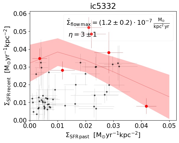
(a)

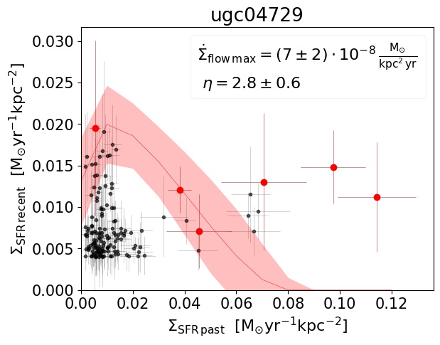
(b)

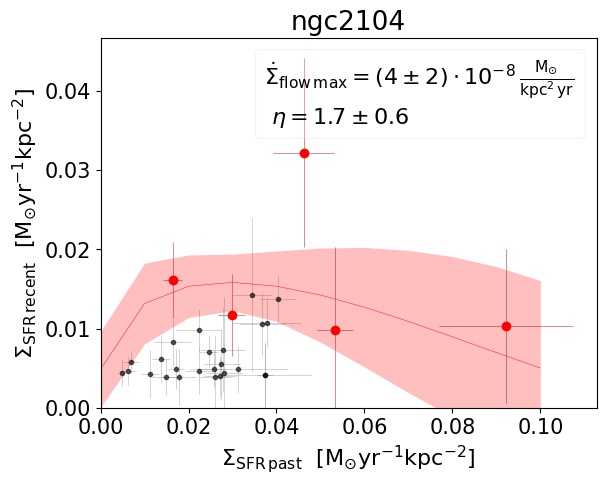
(c)

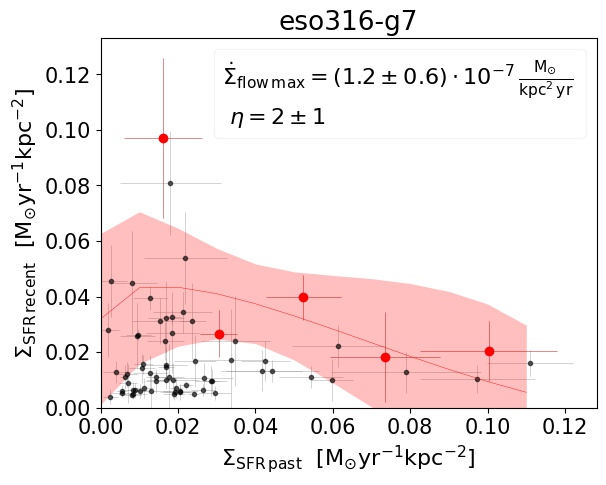
(d)

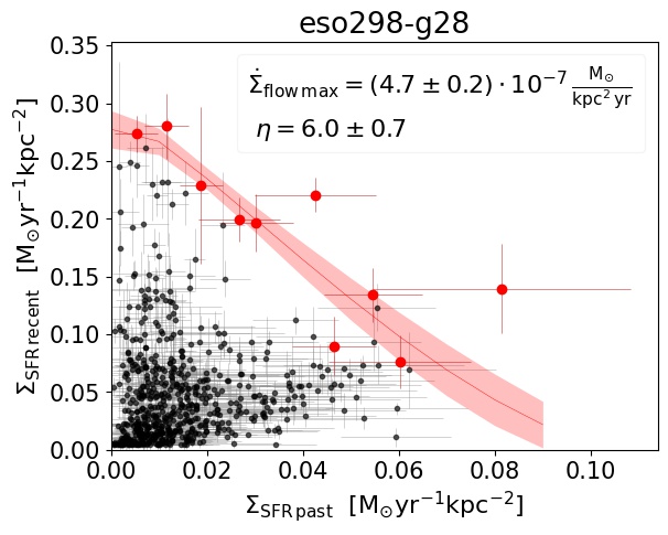
(e)

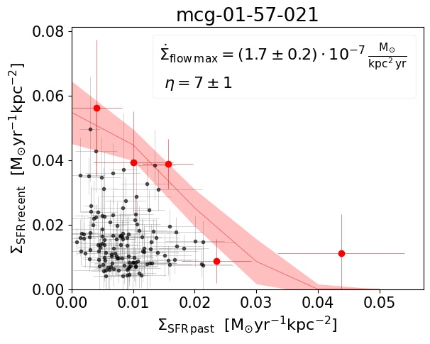
(f)

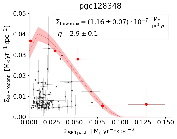
(g)

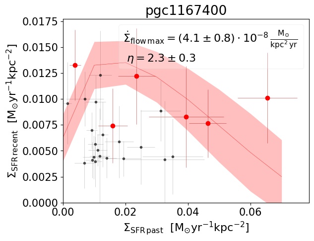
(h)

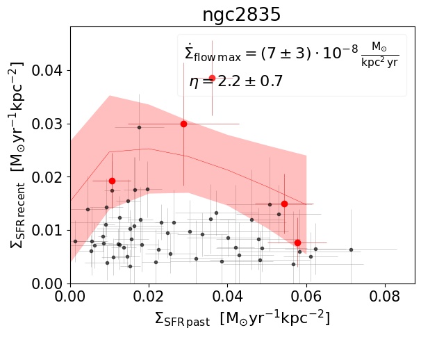
(i)

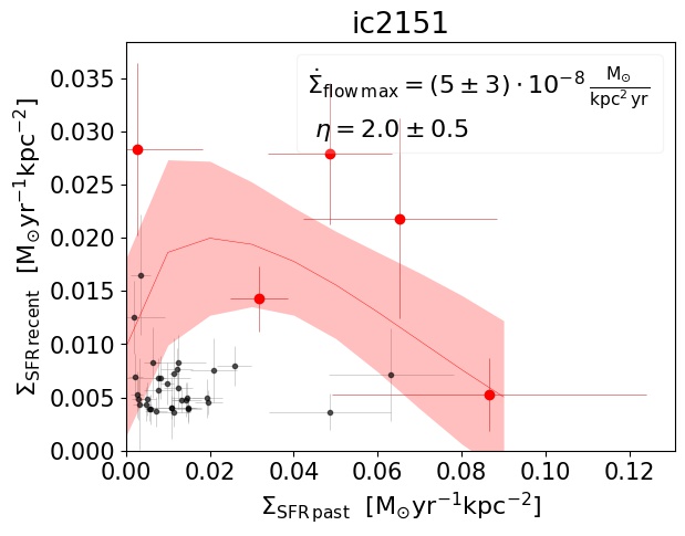
(j)

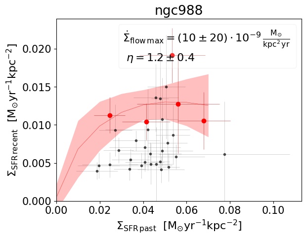
(k)

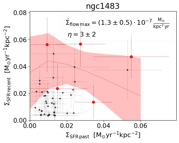
(l)

Figure 9: continued

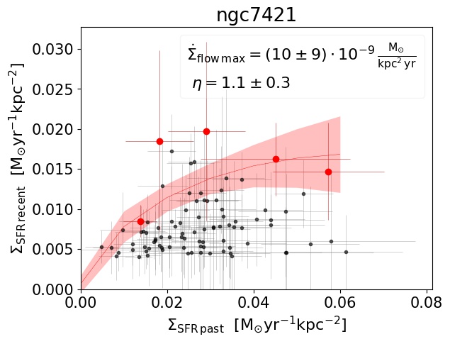
(a)

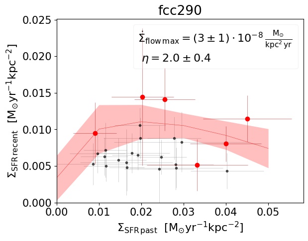
(b)

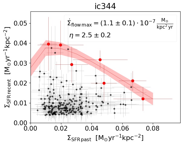
(c)

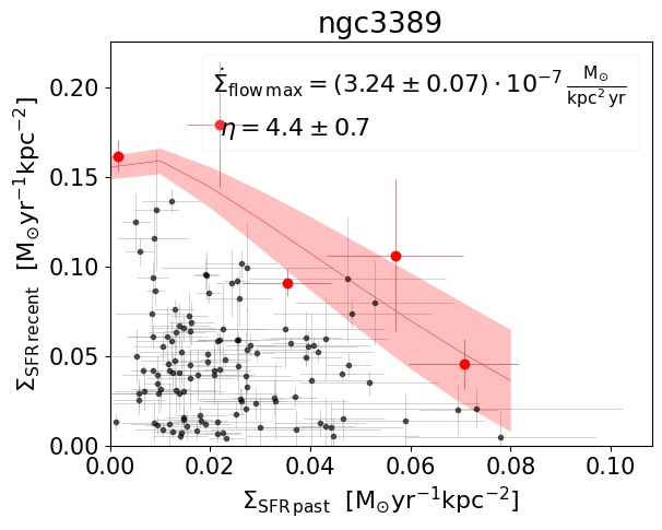
(d)

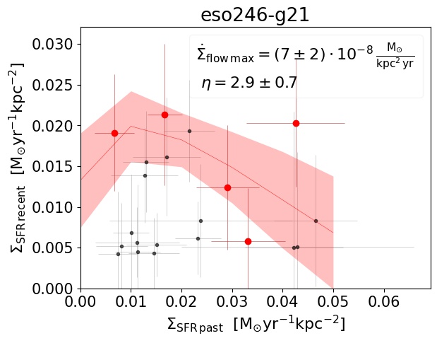
(e)

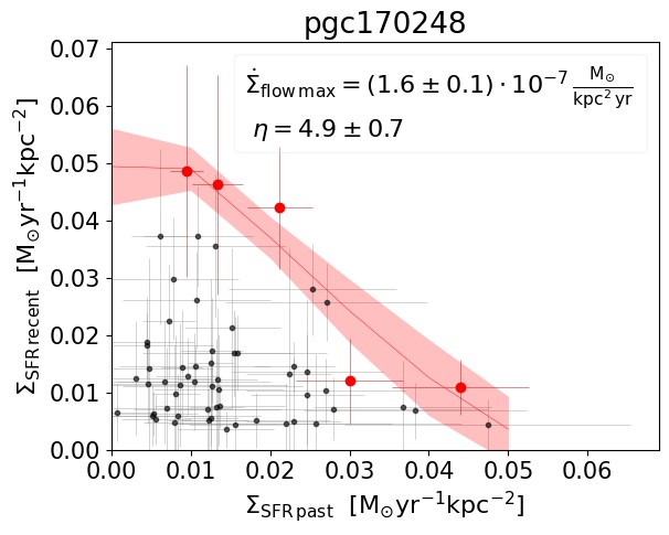
(f)

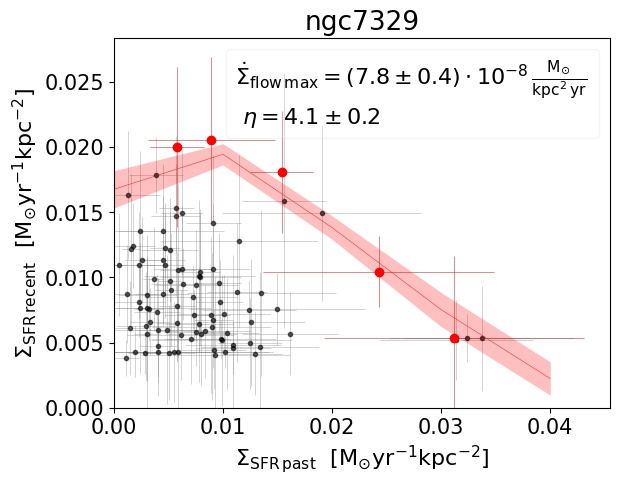
(g)

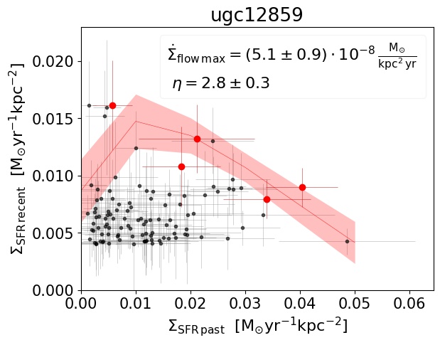
(h)

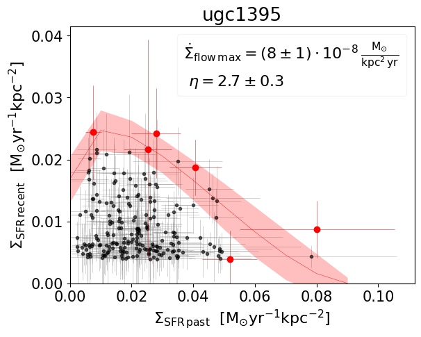
(i)

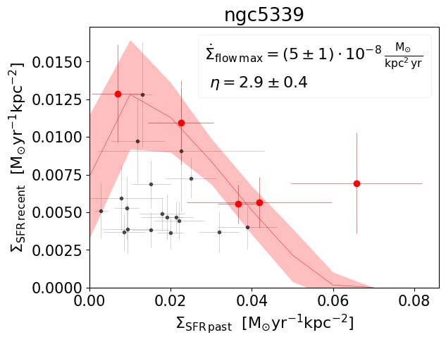
(j)

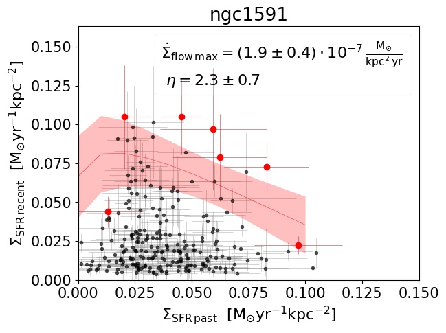
(k)

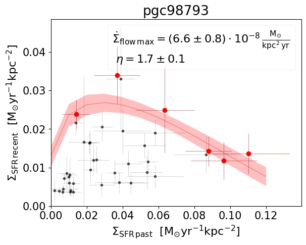
(l)

Figure 10: continued

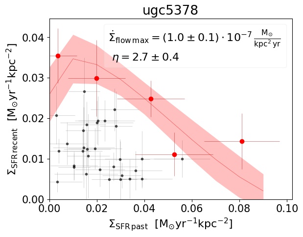
(a)

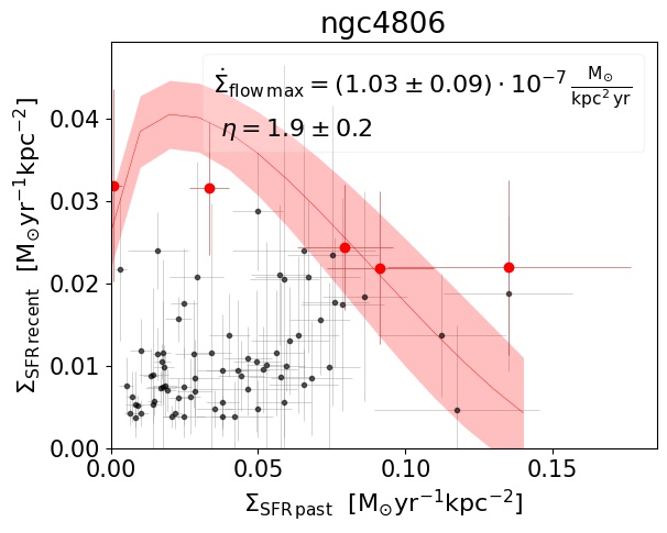
(b)

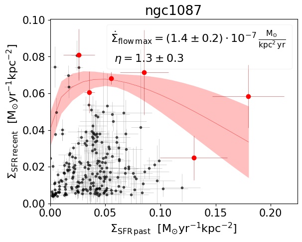
(c)

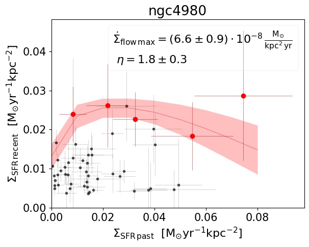
(d)

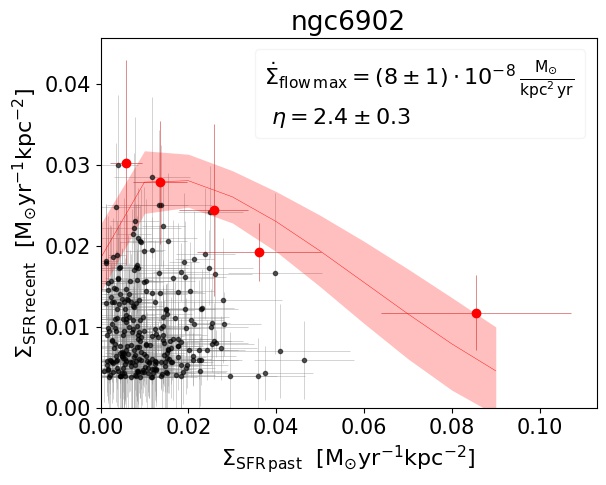
(e)

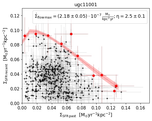
(f)

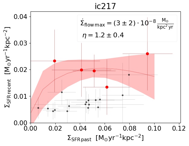
(g)

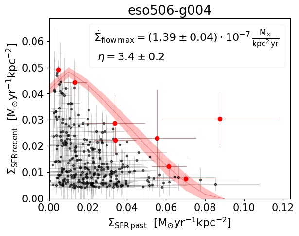
(h)

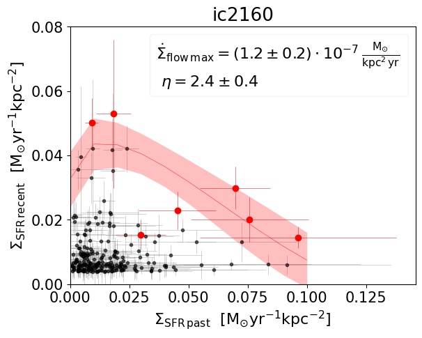
(i)

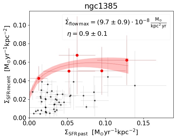
(j)

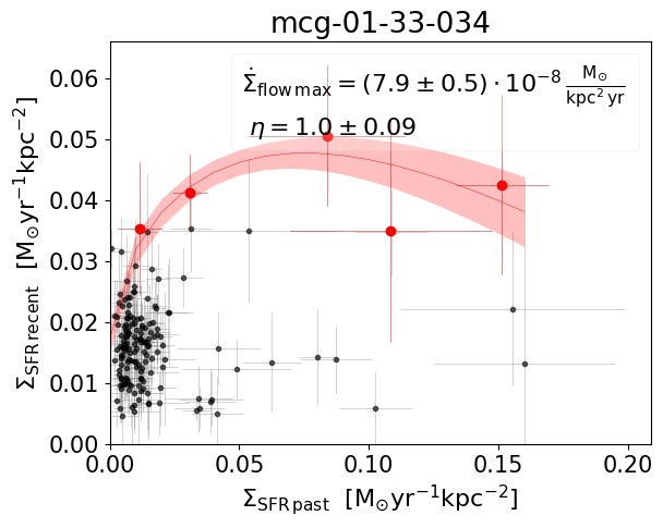
(k)

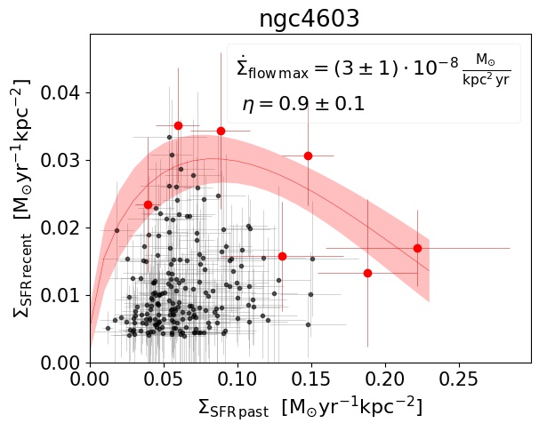
(l)

Figure 11: continued

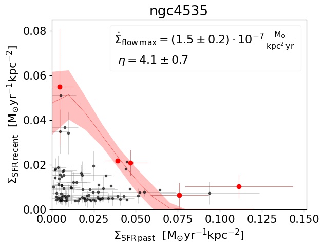
(a)

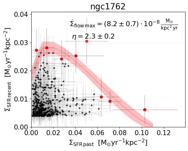
(b)

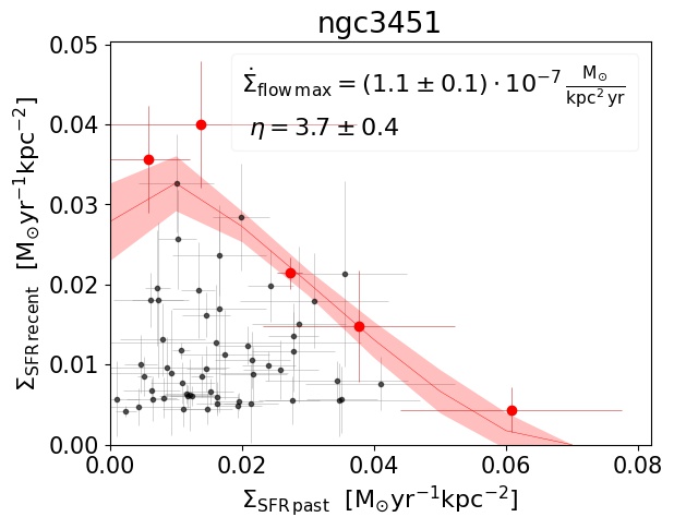
(c)

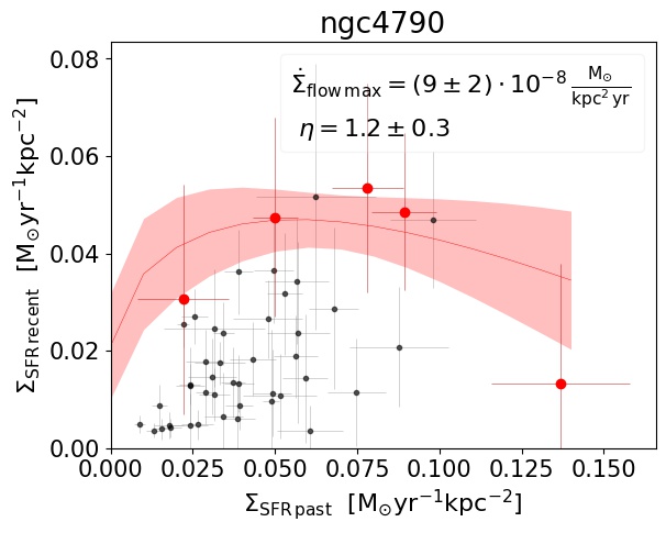
(d)

(e)

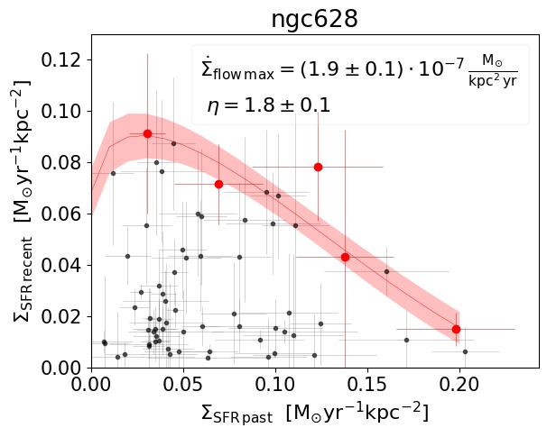
(f)

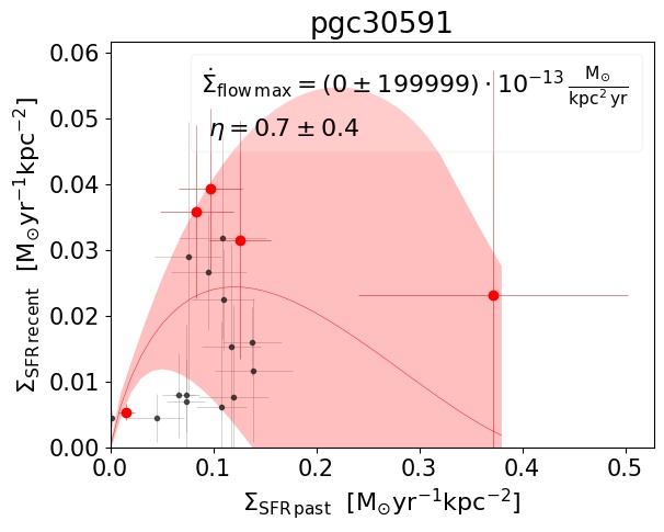
(g)

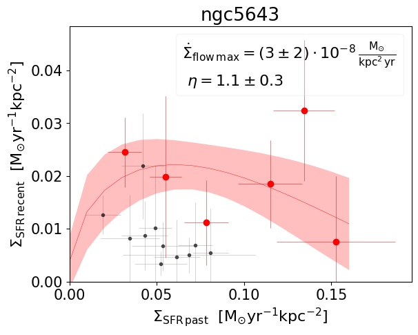
(h)

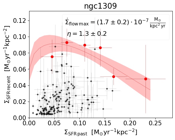
(i)

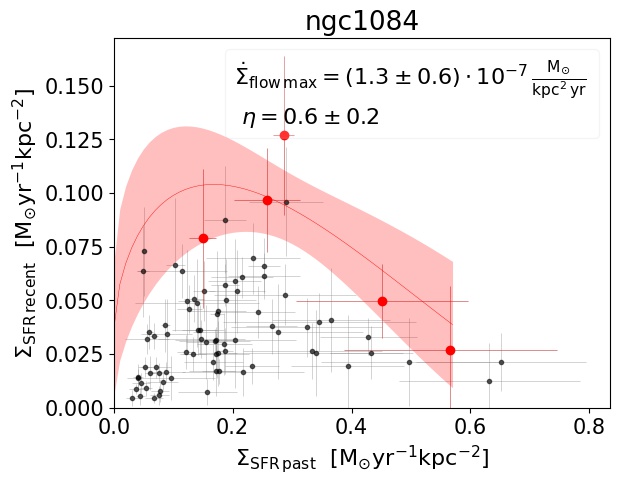
(j)

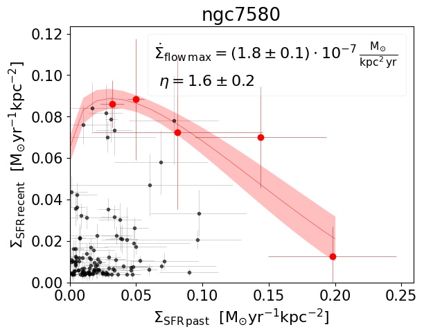
(k)

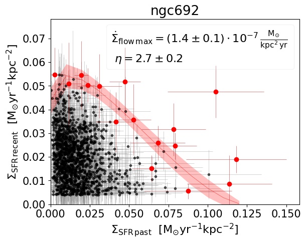
(l)

Figure 12: continued

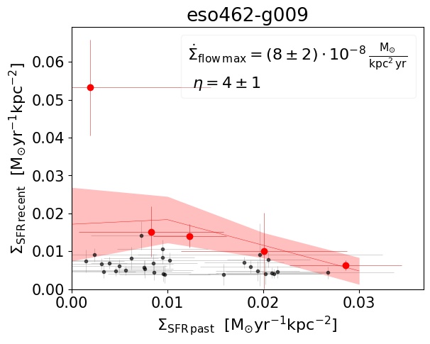
(a)

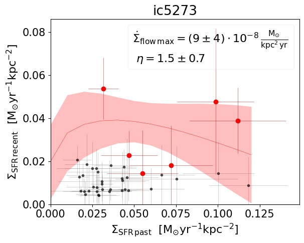
(b)

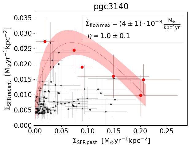
(c)

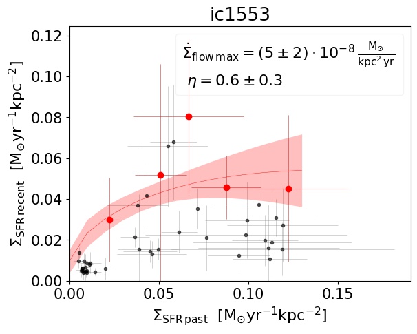
(d)

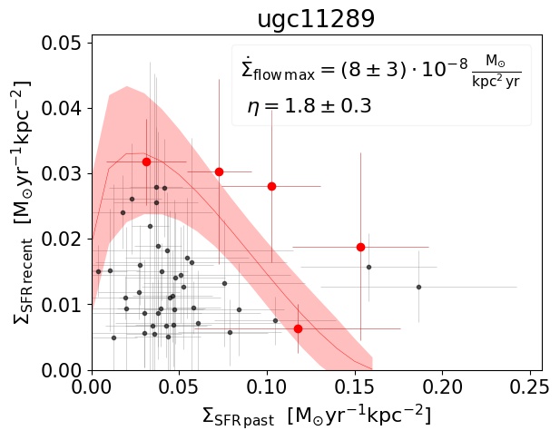
(e)

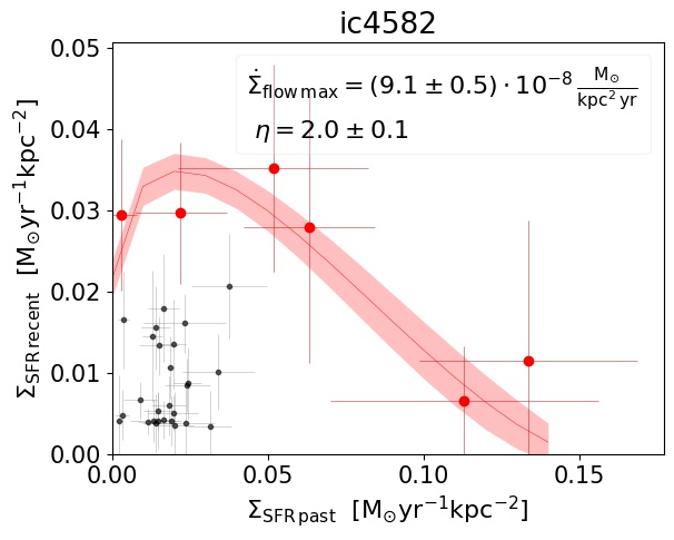
(f)

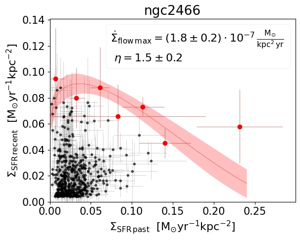
(g)

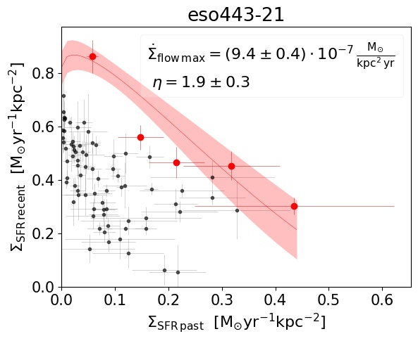
(h)

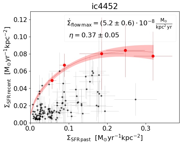
(i)

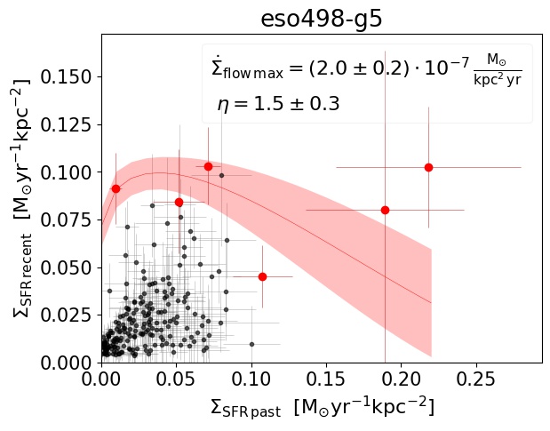
(j)

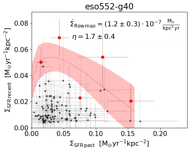
(k)

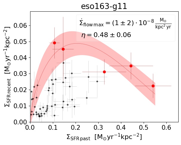
(l)

Figure 13: continued

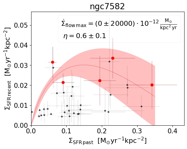
(a)

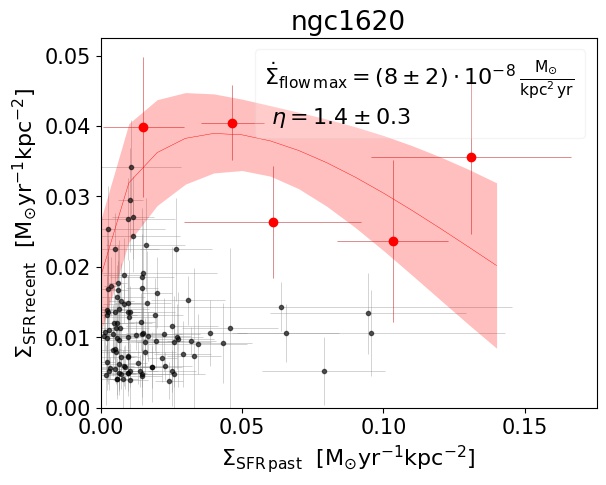
(b)

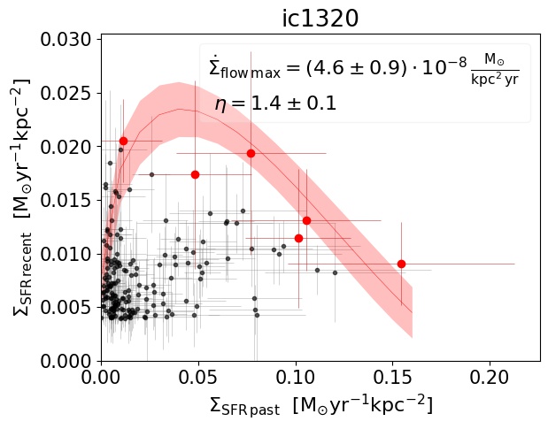
(c)

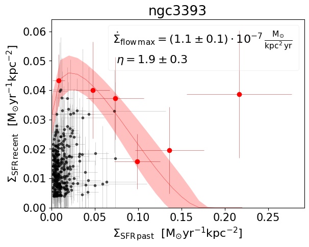
(d)

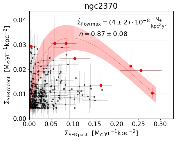
(e)

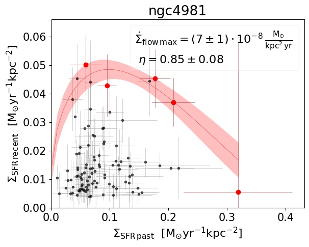
(f)

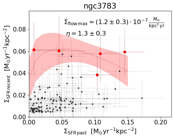
(g)

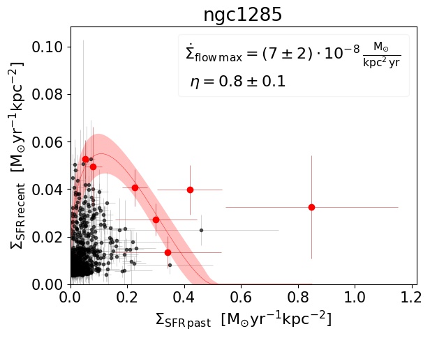
(h)

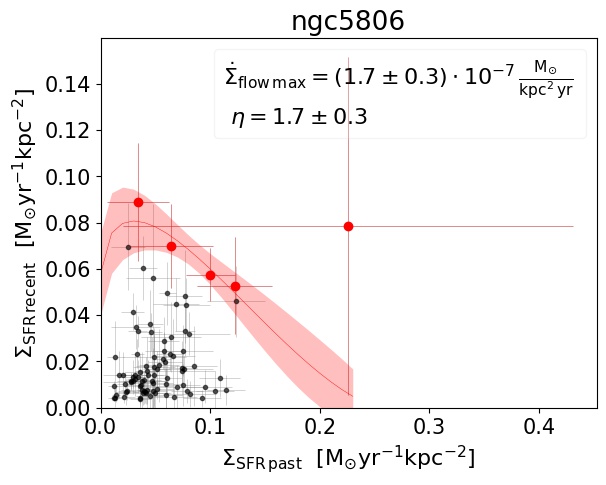
(i)

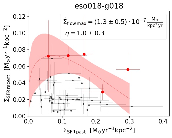
(j)

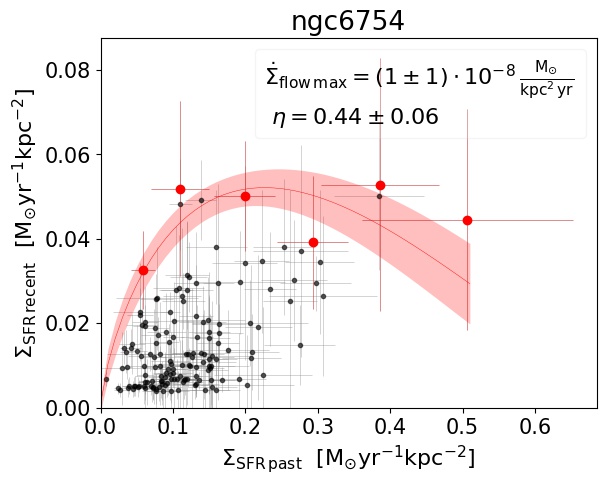
(k)

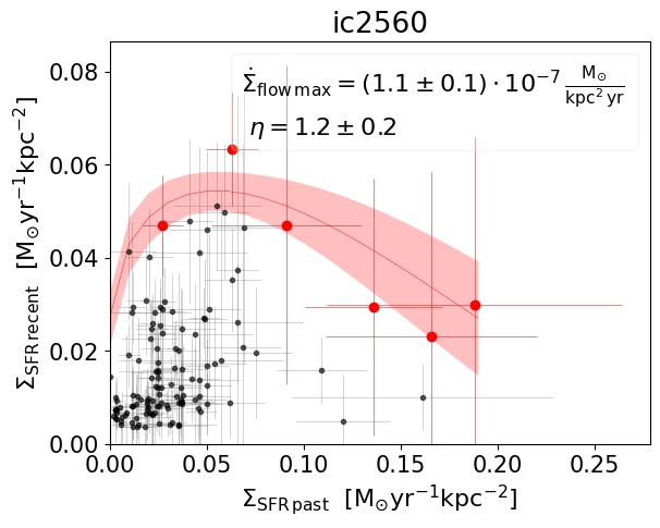
(l)

Figure 14: continued

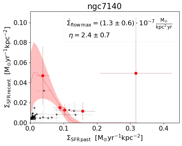
(a)

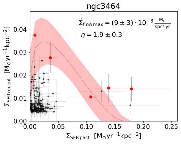
(b)

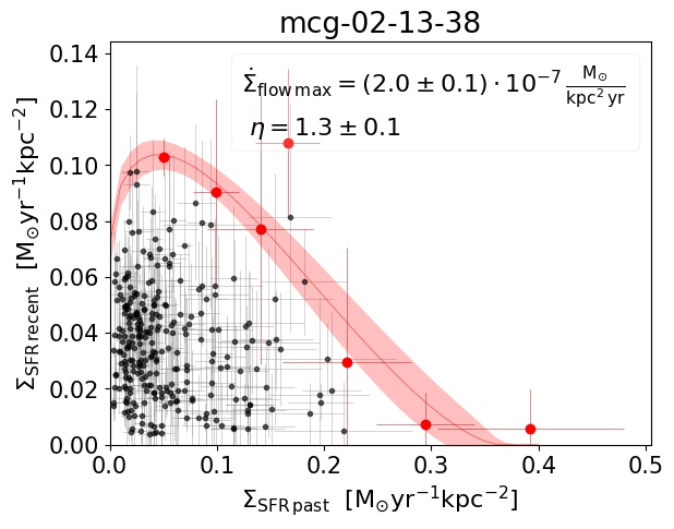
(c)

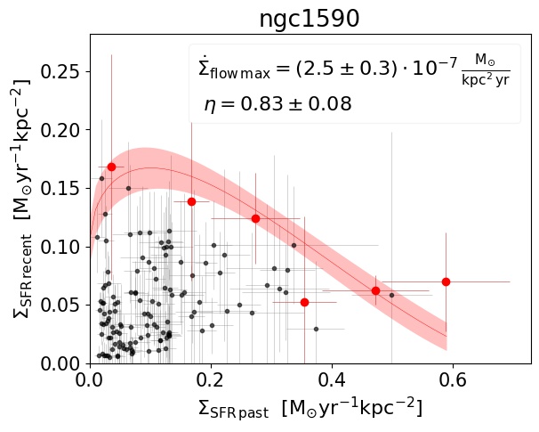
(d)

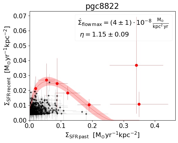
(e)

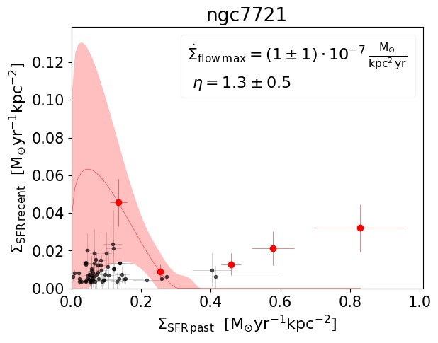
(f)

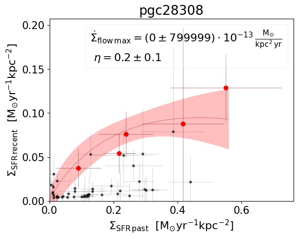
(g)

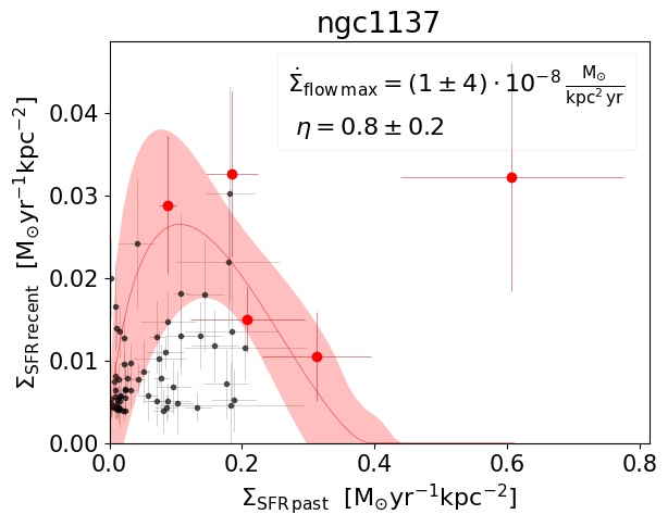
(h)

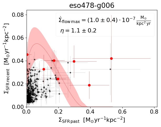
(i)

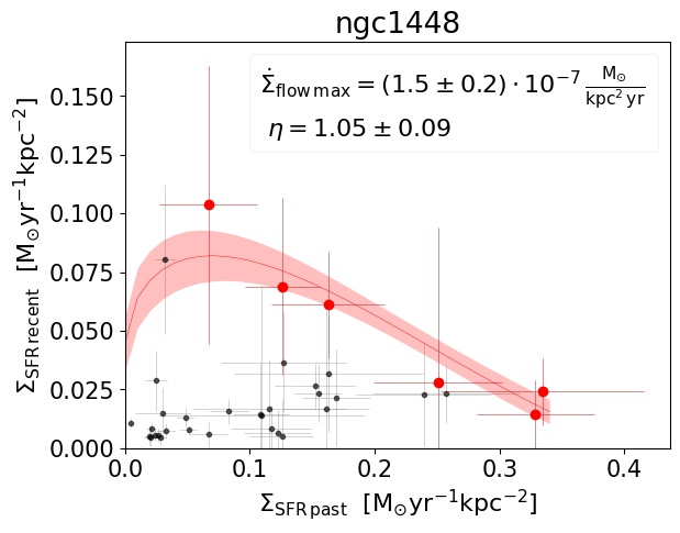
(j)

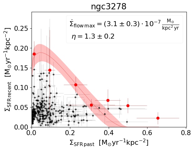
(k)

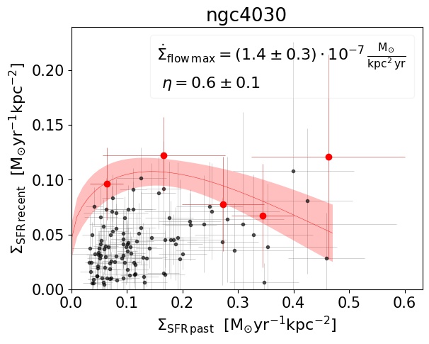
(l)

Figure 15: continued

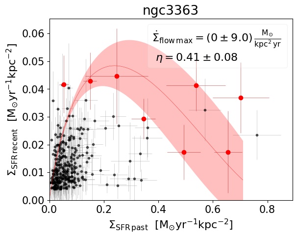
(a)

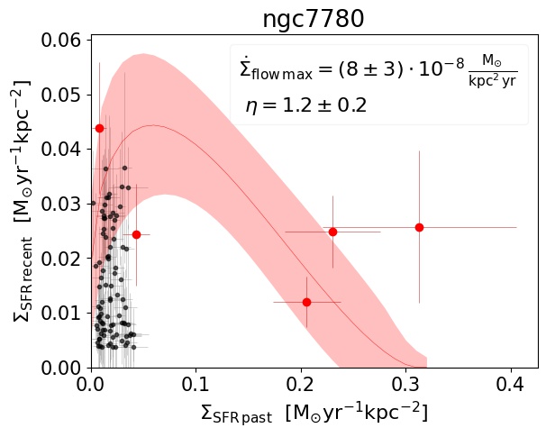
(b)

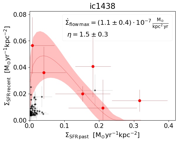
(c)

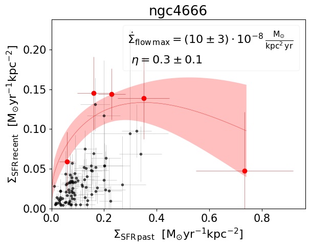
(d)

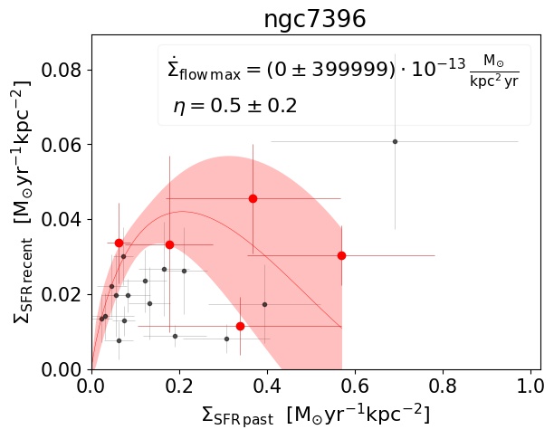
(e)

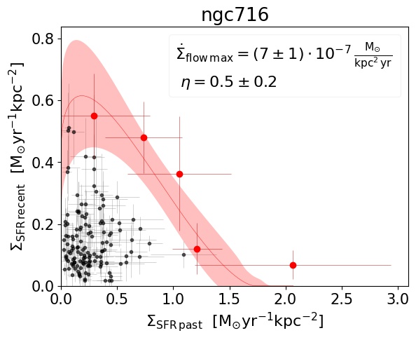
(f)

Figure 16: continued

References

- Arp (1966) Arp H., 1966, ApJS, 14, 1
- Ascasibar et al. (2015) Ascasibar Y., Gavilán M., Pinto N., Casado J., Rosales-Ortega F., Díaz A. I., 2015, MNRAS, 448, 2126
- Astropy Collaboration et al. (2013) Astropy Collaboration et al., 2013, A&A, 558, A33
- Astropy Collaboration et al. (2018) Astropy Collaboration et al., 2018, AJ, 156, 123
- Bacon et al. (2010) Bacon R., et al., 2010, in Proc. SPIE. p. 773508, doi:10.1117/12.856027
- Barrera-Ballesteros et al. (2018) Barrera-Ballesteros J. K., et al., 2018, ApJ, 852, 74
- Barrera-Ballesteros et al. (2020) Barrera-Ballesteros J. K., et al., 2020, MNRAS, 492, 2651
- Behroozi et al. (2010) Behroozi P. S., Conroy C., Wechsler R. H., 2010, ApJ, 717, 379
- Bigiel et al. (2008) Bigiel F., Leroy A., Walter F., Brinks E., de Blok W. J. G., Madore B., Thornley M. D., 2008, AJ, 136, 2846
- Bouché et al. (2010) Bouché N., et al., 2010, ApJ, 718, 1001
- Calzetti et al. (2000) Calzetti D., Armus L., Bohlin R. C., Kinney A. L., Koornneef J., Storchi-Bergmann T., 2000, ApJ, 533, 682
- Camps-Fariña et al. (2015) Camps-Fariña A., Zaragoza-Cardiel J., Beckman J. E., Font J., García-Lorenzo B., Erroz-Ferrer S., Amram P., 2015, MNRAS, 447, 3840
- Cano-Díaz et al. (2019) Cano-Díaz M., Ávila-Reese V., Sánchez S. F., Hernández-Toledo H. M., Rodríguez-Puebla A., Boquien M., Ibarra-Medel H., 2019, MNRAS, 488, 3929
- Chabrier (2003) Chabrier G., 2003, PASP, 115, 763
- Cid Fernandes et al. (2005) Cid Fernandes R., Mateus A., Sodré L., Stasińska G., Gomes J. M., 2005, MNRAS, 358, 363
- Creasey et al. (2013) Creasey P., Theuns T., Bower R. G., 2013, MNRAS, 429, 1922
- Dekel & Mandelker (2014) Dekel A., Mandelker N., 2014, MNRAS, 444, 2071
- Díaz-García et al. (2016) Díaz-García S., Salo H., Laurikainen E., 2016, A&A, 596, A84
- Erroz-Ferrer et al. (2019) Erroz-Ferrer S., et al., 2019, MNRAS, 484, 5009
- Ferland (1993) Ferland G. J., 1993, Hazy, A Brief Introduction to Cloudy 84
- Ferland et al. (1998) Ferland G. J., Korista K. T., Verner D. A., Ferguson J. W., Kingdon J. B., Verner E. M., 1998, PASP, 110, 761
- Ferland et al. (2013) Ferland G. J., Kisielius R., Keenan F. P., van Hoof P. A. M., Jonauskas V., Lykins M. L., Porter R. L., Williams R. J. R., 2013, ApJ, 767, 123
- Forbes et al. (2014) Forbes J. C., Krumholz M. R., Burkert A., Dekel A., 2014, MNRAS, 443, 168
- Fraternali (2017) Fraternali F., 2017, Gas Accretion via Condensation and Fountains. p. 323, doi:10.1007/978-3-319-52512-9_14
- Fritz et al. (2007) Fritz J., et al., 2007, A&A, 470, 137
- Fritz et al. (2011) Fritz J., et al., 2011, A&A, 526, A45
- Fritz et al. (2017) Fritz J., et al., 2017, ApJ, 848, 132
- Ginsburg et al. (2019) Ginsburg A., et al., 2019, AJ, 157, 98
- Hayward & Hopkins (2017) Hayward C. C., Hopkins P. F., 2017, MNRAS, 465, 1682
- Hickson (1982) Hickson P., 1982, ApJ, 255, 382
- Hopkins et al. (2014) Hopkins P. F., Kereš D., Oñorbe J., Faucher-Giguère C.-A., Quataert E., Murray N., Bullock J. S., 2014, MNRAS, 445, 581
- Hopkins et al. (2018) Hopkins P. F., et al., 2018, MNRAS, 480, 800
- Kennicutt et al. (2007) Kennicutt Robert C. J., et al., 2007, ApJ, 671, 333
- Kewley et al. (2006) Kewley L. J., Groves B., Kauffmann G., Heckman T., 2006, MNRAS, 372, 961
- Kormendy & Kennicutt (2004) Kormendy J., Kennicutt Robert C. J., 2004, ARA&A, 42, 603
- Kreckel et al. (2019) Kreckel K., et al., 2019, ApJ, 887, 80
- Kruijssen et al. (2019) Kruijssen J. M. D., et al., 2019, Nature, 569, 519
- Lada & Lada (2003) Lada C. J., Lada E. A., 2003, ARA&A, 41, 57
- Leroy et al. (2019) Leroy A. K., et al., 2019, ApJS, 244, 24
- Li et al. (2017) Li M., Bryan G. L., Ostriker J. P., 2017, ApJ, 841, 101
- Lilly et al. (2013) Lilly S. J., Carollo C. M., Pipino A., Renzini A., Peng Y., 2013, ApJ, 772, 119
- López-Cobá et al. (2020) López-Cobá C., et al., 2020, AJ, 159, 167
- Madau & Dickinson (2014) Madau P., Dickinson M., 2014, ARA&A, 52, 415
- Makarov et al. (2014) Makarov D., Prugniel P., Terekhova N., Courtois H., Vauglin I., 2014, A&A, 570, A13
- Martín-Navarro et al. (2018) Martín-Navarro I., Brodie J. P., Romanowsky A. J., Ruiz-Lara T., van de Ven G., 2018, Nature, 553, 307
- McQuinn et al. (2019) McQuinn K. B. W., van Zee L., Skillman E. D., 2019, ApJ, 886, 74
- Muratov et al. (2015) Muratov A. L., Kereš D., Faucher-Giguère C.-A., Hopkins P. F., Quataert E., Murray N., 2015, MNRAS, 454, 2691
- Osterbrock (1989) Osterbrock D. E., 1989, Astrophysics of gaseous nebulae and active galactic nuclei
- Paturel et al. (2003) Paturel G., Petit C., Prugniel P., Theureau G., Rousseau J., Brouty M., Dubois P., Cambrésy L., 2003, A&A, 412, 45
- Poggianti et al. (2017) Poggianti B. M., et al., 2017, ApJ, 844, 48
- Relaño & Beckman (2005) Relaño M., Beckman J. E., 2005, A&A, 430, 911
- Roberts-Borsani et al. (2020) Roberts-Borsani G. W., Saintonge A., Masters K. L., Stark D. V., 2020, MNRAS, 493, 3081
- Robitaille & Bressert (2012) Robitaille T., Bressert E., 2012, APLpy: Astronomical Plotting Library in Python (ascl:1208.017)
- Rodríguez-Puebla et al. (2016) Rodríguez-Puebla A., Primack J. R., Behroozi P., Faber S. M., 2016, MNRAS, 455, 2592
- Sánchez-Menguiano et al. (2018) Sánchez-Menguiano L., et al., 2018, A&A, 609, A119
- Sánchez et al. (2016) Sánchez S. F., et al., 2016, Rev. Mex. Astron. Astrofis., 52, 21
- Schaye et al. (2010) Schaye J., et al., 2010, MNRAS, 402, 1536
- Schroetter et al. (2015) Schroetter I., Bouché N., Péroux C., Murphy M. T., Contini T., Finley H., 2015, ApJ, 804, 83
- Schroetter et al. (2019) Schroetter I., et al., 2019, MNRAS, 490, 4368
- Silk & Mamon (2012) Silk J., Mamon G. A., 2012, Research in Astronomy and Astrophysics, 12, 917
- Somerville & Davé (2015) Somerville R. S., Davé R., 2015, ARA&A, 53, 51
- Vogelsberger et al. (2013) Vogelsberger M., Genel S., Sijacki D., Torrey P., Springel V., Hernquist L., 2013, MNRAS, 436, 3031
- Vorontsov-Velyaminov (1959) Vorontsov-Velyaminov B. A., 1959, Atlas and Catalog of Interacting Galaxies (1959, p. 0
- Werle et al. (2019) Werle A., Cid Fernandes R., Vale Asari N., Bruzual G., Charlot S., Gonzalez Delgado R., Herpich F. R., 2019, MNRAS, 483, 2382
- Zaragoza-Cardiel et al. (2019) Zaragoza-Cardiel J., et al., 2019, MNRAS, 487, L61