Convex Shape and Rotation Model of Lucy Target (11351) Leucus
from Lightcurves and Occultations

Abstract

We report new photometric lightcurve observations of the Lucy Mission target (11351) Leucus acquired during the 2017, 2018 and 2019 apparitions. We use these data in combination with stellar occultations captured during five epochs (Buie et al., 2020) to determine the sidereal rotation period, the spin axis orientation, a convex shape model, the absolute scale of the object, its geometric albedo, and a model of the photometric properties of the target. We find that Leucus is a prograde rotator with a spin axis located within a sky-projected radius of 3$\arcdeg$ (1$\sigma$) from J2000 Ecliptic coordinates ($\lambda=208\arcdeg$, $\beta=+77\arcdeg$) or J2000 Equatorial Coordinates (RA=248$\arcdeg$, Dec=+58$\arcdeg$). The sidereal period is refined to $P_{sid}=445.683\pm 0.007$ h. The convex shape model is irregular, with maximum dimensions of (60.8, 39.1, 27.8) km. The convex model accounts for global features of the occultation silhouettes, although minor deviations suggest that local and global concavities are present. We determine a geometric albedo $p_{V}=0.043\pm 0.002$. .

1 Introduction

Jupiter Trojans are a class of small objects trapped in the Jupiter L4 and L5 Lagrangian points. Their origin is still disputed, with the most likely scenarios falling into the categories 1) coeval trapping of local planetesimals in the 1:1 mean motion resonance with accreting Jupiter as a consequence of drag or collisions (Yoder, 1979; Shoemaker et al., 1989) or 2) post Jupiter-formation capture of scattered trans-Neptunian planetesimals following an episode of orbital chaos (Morbidelli et al., 2005) during the orbital migration of the giant planets or as a consequence of the Jumping Jupiter scenario as defined in Nesvorný et al. (2013). In either cases, Trojans are thought to be primitive objects that experienced little thermal evolution and contain a considerable amount of volatiles, which makes them close relatives to cometary nuclei.

With a launch planned for October 2021, Lucy is the thirteenth NASA mission of the Discovery Program and will be the first one to explore the Jupiter Trojan System. Its trajectory is designed to fly-by 5 Trojans – one of which, (617) Patroclus is an equal-size binary system – distributed over the two Lagrangian clouds. The encounter with Leucus is currently planned for June 18, 2028. A coordinated effort has been initiated to support the mission with a systematic program of ground-based observations of the mission targets aiming at characterizing their dynamical, physical, rotational and photometric properties. The goal is to inform the mission design in order to maximize the scientific return of the encounters and to complement the space-based measurements with data that are most efficiently acquired from the ground.

This paper presents new lightcurve photometry of the Lucy target Leucus, which is used, together with the results of stellar occultation campaigns presented in a companion paper (Buie et al., 2020), to determine its convex shape, spin axis orientation, albedo, size, sphere-integrated phase curve and V–R color index.

2 Leucus

(11351) Leucus belongs to the Jupiter L4 Trojan swarm. Radiometric measurements by the IRAS satellite reported a size and a geometric albedo of 42.2$\pm{4.0}$ km and 0.063$\pm{0.014}$, respectively (Tedesco et al., 2004). Grav et al. (2012), reported size and albedo of 34.155$\pm{0.646}$ km and 0.079$\pm{0.013}$, respectively, based on WISE radiometry. Levison & Lucy Science Team (2016) classified Leucus tentatively as belonging to the D taxonomic type, . No collisional family membership has been proposed as of today. French et al. (2013) first realized from lightcurve data that Leucus is a very slow rotator, although they identified an incorrect period of 515 h. Buie et al. (2018), by using photometric observations acquired during the 2016 apparition, combined with the observations by French, determined a firm rotation period of 445.732 $\pm$ 0.021 h. They also estimated a geometric albedo of 0.047 based on the WISE diameter and on an average color index for D-type asteroids.

3 Observations and data reduction

The new Leucus photometric observations reported in this paper were performed during its 2017, 2018 and 2019 apparitions by using 1.0 m telescopes from the Las Cumbres Observatory Global Telescope (LCOGT) network, the 1.2 m telescope at the Calar Alto Observatory, Spain, and the two 24^′′ telescopes sited at Sierra Remote Observatories (SRO), Auberry, CA, USA, owned and operated by SwRI. The observational circumstances are detailed in Table 1. Typical exposure times were of 5 min for the Calar Alto observations, with the telescope tracked at half the relative tracking rate of the asteroid, in order reduce smearing and obtain equal point-spread functions for the target and field stars. The LCOGT observations were also exposed for typically 5 min, but were tracked at object rate, since those telescopes do not support halfway tracking.

The SRO systems use an Andor Xyla sCMOS camera with a maximum exposure time of 30 seconds. All data taken on Leucus used this maximum exposure time. In 30 seconds, the motion of Leucus is 125 mas at opposition, corresponding to less than a half of a pixel smear and and even smaller fraction of the point-spread function (PSF). The very fast readout and low read noise of the sCMOS camera nearly eliminate the penalties of taking such short exposures. During processing, we can stack as many images as desired to reach a SNR goal. Two stacks are built from the data, one registered on the stars and the other registered on the apparent motion of Leucus. We can use image subtraction to remove the stars in the Leucus stack but this was not necessary for the 2018 and 2019 data from SRO. For these data we chose to stack 10 images at a time and used synthetic aperture integration to retrieve the photometry of Leucus, thus providing an effective integration over 5 minutes. The star-stacked images were used with the same aperture to determine the instrumental magnitudes of the stars.

This raw photometry was further binned in time by a factor of 3 to increase the per-point SNR while also allowing the estimation of a good uncertainty for the photometry.

For the observations from Calar Alto, most fields were measured with Himmelspolizey, a reduction pipeline developed by SH. The latter implements a semi-automatic astrometric/photometric workflow that uses SExtractor (Bertin & Arnouts, 1996) for photometric extraction, an optimistic pattern matching algorithm (Tabur, 2007) for astrometric reduction and a moving object detection algorithm for asteroid identification as described in Kubica et al. (2007). In the case of crowded fields, synthetic aperture photometry was measured interactively with AstPhot (Mottola et al., 1995).

The observations proved to be challenging mainly because of two aspects. First, during the 2017 apparition the target was still close to the Galactic center, which implied that involvement of the source with field stars was extremely frequent. This issue was dealt with by applying star subtraction. For the observations taken from the LCOGT Network the subtraction was performed in the image domain, by applying the method described in Buie et al. (2018). For the observations from Calar Alto, the subtraction was performed in the intensity domain, by separately measuring the flux of the involved stars at many epochs distant from the time of the respective appulses. Although star subtraction mitigates the contamination problem, it is not a perfect solution. While the flux of the polluting star is removed, the photon noise associated to the subtracted flux still contributes to the degradation of the total SNR, sometimes being the dominant contribution. In the latter cases the affected frames were excluded altogether from the data set. Furthermore, imperfect background source removal, due e.g. to changing seeing conditions during the observations, results in a non-Gauss distribution of the measurements error which can cause outliers in the data that can be difficult to discern.

The second challenging aspect was represented by the very long rotation period of the target, which caused a useful night of observations to produce data points only at a single rotational aspect. As a consequence, a large number of nights over extended periods of time were needed to ensure complete rotational coverage. Furthermore, the resulting data set virtually consisted only of sparse photometry, in the sense that subsequent nights’ observations didn’t overlap in rotation phase, preventing a composite lightcurve to be compiled from relative photometry. Composite lightcurves were therefore generally constructed based on absolute photometry, with the disadvantage of the additional uncertainty component due to the errors of the calibration zero points. Fortunately, modern, all-sky photometric catalogs with very good coverage, limiting magnitude and accuracy have become available in recent times, so that the problem of the accuracy of the zero point is not as severe as in the past. With the fields of view of our detectors, a large number of suitable photometric catalog stars was always simultaneously present in the same frame as the target, allowing us to identify variable stars and outliers. For the observations from LCOGT, carried out with the SDSS r’ filter, we used the APASS photometric catalog (Henden et al., 2012). For the Calar Alto observations, carried out in the Johnson V and Cousins R_C filters, we used the GAIA DR2 catalog with the transformations from the G photometric band from Evans et al. (2018). The observations from the SRO were performed with a VR broadband filter. Gaia DR2 field stars were used to directly express the asteroid in the Gaia G bandpass without further transformation or color correction.

Typically, relative photometric accuracy of the individual points (binned points for the SRO) ranged from 0.01 to 0.03 mag RMS. The absolute photometric accuracy of the zero points was typically of the order of 0.02 mag RMS.

For the purpose of compact representation – but not for model computation – the photometric time series were compiled into composites for each individual apparition. This was achieved by performing a Fourier series fit of the fourth order to determine the respective best-fit synodic periods by using the procedure described in Harris et al. (1989). Normally, we would fit simultaneously the Fourier coefficients and a phase function to absolute photometry data, in order to compensate for brightness changes due to the phase curve. The implicit assumption is that the shape of the lightcurve – in particular its amplitude – remains constant over a few consecutive rotational cycles. While this is a reasonable assumption for most asteroids, in the case of Leucus, given its very slow rotation, the amplitude of the lightcurve can change over consecutive rotational cycles due to the change in viewing and observing geometry. Fitting the phase function simultaneously with the rotation period would tend to compensate the change in the lightcurve amplitude by skewing the phase function, which could result in varying phase curve slopes for different apparitions. For this reason we performed the composites with a nominal linear phase coefficient $\beta=0.0395$ $mag/\arcdeg$ for all of the observations reported in this paper .

The composite lightcurves for the 2017, 2018 and 2019 apparitions are reported in Figure 1. It can be seen that the respective synodic periods differ among each other by as much as 0.7 h, which corresponds to about 0.15%. This is expected for two lines of reasons. First, due to the slow rotation, the useful baseline for the determination of the periods for each apparition just covers a handful of rotational cycles, which limits the accuracy of the determination. Secondly – and to a lesser extent – the apparent instantaneous rotation rate depends on the rate of change of the topocentric ecliptic longitude of the object, which can make the synodic period change slightly during the course of an appartition and from one apparition to the next. In the next sections we will derive a very accurate sidereal period and phase function, by using a dynamical and shape model that makes use of all of the available observations, over a baseline of about 6 years.

Table 1: Observational circumstances

Date	$\lambda$	$\beta$	$\alpha$	r	$\Delta$	$\lambda$ (PAB) $\beta$		Band	Observatory	Observers
(UT)	($\arcdeg$ J2000)		($\arcdeg$)	(au)	(au)	($\arcdeg$ J2000)
2017 May 1.1	287.4	+5.7	9.683	5.5071	5.0320	282.5	+5.5	RC	493	SH, SMo
2017 May 2.1	287.4	+5.8	9.616	5.5067	5.0175	282.6	+5.5	RC	493	SH, SMo
2017 May 20.1	287.0	+6.3	7.887	5.5005	4.7745	283.0	+5.9	RC	493	SH, SMo
2017 May 28.1	286.5	+6.6	6.841	5.4977	4.6852	283.1	+6.1	RC	493	SMo, SH
2017 May 30.1	286.3	+6.6	6.550	5.4970	4.6646	283.1	+6.1	RC	493	SMo, SH
2017 May 31.0	286.3	+6.6	6.408	5.4966	4.6551	283.1	+6.1	RC	493	SMo, SH
2017 Jul 16.4	281.0	+7.6	2.738	5.4798	4.4914	282.2	+6.9	r’	Q64	MWB, AZ
2017 Jul 17.0	280.9	+7.6	2.833	5.4795	4.4932	282.1	+6.9	r’	W86	MWB, AZ
2017 Jul 17.3	280.9	+7.6	2.882	5.4794	4.4942	282.1	+6.9	r’	W85	MWB, AZ
2017 Jul 17.6	280.8	+7.6	2.933	5.4793	4.4952	282.1	+6.9	r’	Q63	MWB, AZ
2017 Jul 17.9	280.8	+7.6	2.980	5.4792	4.4962	282.1	+6.9	r’	K93	MWB, AZ
2017 Jul 18.2	280.8	+7.6	3.031	5.4791	4.4973	282.1	+6.9	r’	W86	MWB, AZ
2018 Jun 11.1	318.3	+11.1	9.382	5.3394	4.7451	313.5	+10.5	RC	493	SH, SMo
2018 Jul 9.1	316.6	+12.1	5.829	5.3263	4.4379	313.8	+11.1	V	493	SH, SMo
2018 Jul 15.0	316.0	+12.2	4.895	5.3236	4.3947	313.8	+11.2	V	493	SH, SMo
2018 Sep 4.9	309.8	+12.5	6.171	5.2990	4.4362	312.8	+11.5	V	493	SH, SMo
2018 Aug 6.9	313.2	+12.7	2.406	5.3127	4.3186	313.3	+11.5	RC	493	SH, SMo
2018 Aug 8.0	313.1	+12.7	2.432	5.3123	4.3187	313.3	+11.5	RC	493	SH, SMo
2018 Aug 9.0	312.9	+12.7	2.475	5.3118	4.3192	313.3	+11.5	RC	493	SH, SMo
2019 Nov 9.1	342.2	+12.6	10.103	5.1016	4.5976	347.3	+12.0	VR	G80	MWB
2019 Nov 10.1	342.2	+12.6	10.181	5.1012	4.6112	347.4	+12.0	VR	G80	MWB
2019 Nov 11.1	342.2	+12.5	10.257	5.1008	4.6249	347.4	+12.0	VR	G80	MWB
2019 Nov 12.1	342.2	+12.5	10.329	5.1004	4.6387	347.5	+11.9	VR	G80	MWB
2019 Nov 24.1	342.6	+12.0	10.962	5.0955	4.8123	348.2	+11.7	VR	G80	MWB

Note. — This table is an excerpt. The observational circumstances for all of the observation nights are reported in the online material. $\lambda$ and $\beta$ are the topocentric ecliptic longitude and latitude of the target, respectively. $\alpha$ is the solar phase angle, r is the heliocentric distance and $\Delta$ is the topocentric range of Leucus. $\lambda$ and $\beta$ (PAB) are the topocentric ecliptic longitude and latitude of the phase angle bisector, as defined in Harris et al. (1984)

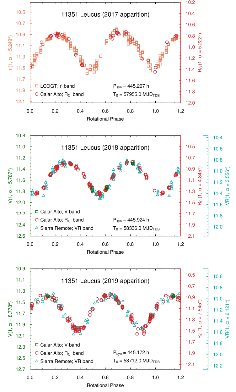
Figure 1: Composite lightcurves for the 2017, 2018 and 2019 apparitions. The data points are folded with the synodic periods listed in the respective graphs, with zero phase corresponding to the respective T₀ epochs. T₀ are one-leg, light-travel time corrected Modified Julian Dates (MJD) expressed in the TDB uniform time frame. The listed synodic periods are the exact numbers used for folding the composites, and as such, are reported without uncertainty. Data points beyond rotation phase 1.0 are repeated for clarity. The magnitudes are reduced to 1 au from the observer and from the Sun and to the respective reference phase angles by using a nominal linear phase coefficient $\beta=0.0395$ mag/$\arcdeg$.

4 Modeling

4.1 Data

The photometric lightcurves presented in the previous section and in Buie et al. (2018), and the results from the stellar occultation campaigns reported in Buie et al. (2020) constitute the bulk of observational data used for our modeling work. In addition, we made use of dense lightcurve photometry by French et al. (2013) (retrieved through the ALCDEF service (http://alcdef.org/)) and sparse photometry from the following sources:

1. The Gaia DR2 database (Gaia Collaboration et al., 2018) retrieved through the VizieR server (https://vizier.u-strasbg.fr/),

2. The ZTF project (Bellm et al., 2019) retrieved through the IRSA server (https://irsa.ipac.caltech.edu/applications/ztf/) and from the nightly transient archive at https://ztf.uw.edu,

3. The PAN-STARRS-1 DR2 database (Flewelling et al., 2016) retrieved through a query to the MAST archive (https://catalogs.mast.stsci.edu/), and

4. The ATLAS project (Tonry et al., 2018) retrieved through the AstDys database (https://newton.spacedys.com/astdys/).

Since the survey observations were acquired in a variety of different photometric systems, for which transformations to the Johnson system are not accurately established, they were treated as relative photometry. Although these additional datasets provide varying degrees of accuracy, they proved to be very useful to extend the coverage and baseline of the observations, which combined, cover a period of about 6 years.

4.2 Convex inversion

In this paper we apply the convex shape inversion approach described in Kaasalainen et al. (2002) and references therein to the photometric time series to simultaneously solve for the sidereal period, the spin axis orientation, the photometric function and a convex, polyhedral approximation of the shape. The occultation data are used as a constraint to resolve the spin axis ambiguity, to determine the scale of the object – and hence its albedo – and to refine the orientation of the spin axis. Although it is likely that Leucus does contain some degree of global-scale concavity, we did not feel that the available data – both because of coverage and photometric accuracy, in the case of lightcurve data, and because of limited unique observation geometries in the case of occultation data – would allow addressing of the intrinsic non-uniqueness of the non-convex problem. On the other hand, the convex inversion scheme offers the advantage of a provably convergent method that results in a unique solution in the case of a convex shape (Kaasalainen & Lamberg, 2006), and gracefully degrades in the case of moderate concavities. Non-convex modeling of Leucus will be the subject of future work as soon as more data – especially at further occultation geometries – become available.

The surface brightness of the object is described through its photometric function, which, for the purpose of this work, is assumed to be separable into a disk function and a surface phase function (see e.g. Schröder et al. 2013). Following Kaasalainen et al. (2001), we adopt Lommel-Seelinger-Lambert (LSL) scattering as a disk function and a 3-parameter exponential-linear combination as a surface phase function, as described in Appendix A. The LSL disk function is the linear combination of the Lommel-Seeliger and Lambert scattering functions through a partition parameter $c$, and is equivalent to the Lunar-Lambert disk function (Li et al. 2015 and references therein) when the latter is used with a partition function independent on the phase angle. We fixed $c$ parameter to a constant value $c=0.1$, appropriate for dark asteroids (Kaasalainen et al., 2005). For this work we didn’t attempt to use more complex photometric models – as e.g. the Hapke function (Hapke 2012 and references therein) – because, due to the small phase angle range in which Trojans can be observed from Earth, no meaningful retrieval of the model parameters is achievable.

The brightness of the object depends on the product of its size and its albedo. From unresolved photometric measurements alone, it is not possible to retrieve independently those two quantities. Independent measurements as thermal radiometry, stellar occultations or direct imaging, however, offer the possibility to disentangle the two quantities. In absence of more detailed information, we assume that the photometric properties of the target – in particular its albedo – are uniform over its surface. This is quite a reasonable assumption to be made, because, although albedo variations on asteroids do occur, the observed lightcurve variations tend to be dominated by the changing cross section of a non-spherical shape.

The convex inversion scheme models the brightness of the target in the space of its Extended Gaussian Image (EGI, Kaasalainen & Torppa 2001), as opposed to the 3D object space. The EGI represents the discrete equivalent of the inverse of the Gaussian Surface Density, and is used to represent the area of the facets oriented towards a particular direction. For the Leucus model we parametrize the EGI with a spherical harmonic expansion of rank and order 8, which results in a total of 81 shape parameters, one of which represents its scale. An exponential-function representation of the EGI is used for guaranteeing the positiveness of the surface areas. We integrate the EGI over the unit sphere by sampling the spherical harmonics expansion at discrete points by following a Lebedev quadrature (Lebedev & Laikov, 1999), which offers greater efficiency compared to a quadrature based, e.g. on a uniform or random sampling (Kaasalainen et al., 2012). In the case of Leucus we applied a Lebedev rule of order 302, which results in an EGI with the same number of facets.

In the case of absolute observations, the optimization is performed by minimizing the reduced $\chi^{2}_{red}$ metric defined as

$$\chi_{red}^{2}=\frac{1}{N}\sum\limits_{i}{\frac{(L_{i}^{obs}-L_{i}^{mod})^{2}}{\sigma_{i}^{2}}}$$ (1)

where $L_{i}^{obs}$ and $L_{i}^{mod}$ are the observed and model intensities, respectively, $\sigma_{i}$ are the intensity uncertainties and $N$ is the number of degrees of freedom for errors. The index $i$ runs over all of the $n$ photometric data points.
In the case of relative observations, we minimize the deviations of the intensities relative to the average of the respective lightcurve:

$$\chi_{rel}^{2}=\frac{1}{N}\sum\limits_{k,j}\left(\frac{\bar{L}^{obs}_{j}}{\sigma_{k,j}}\right)^{2}\left(\frac{L_{k,j}^{obs}}{\bar{L}^{obs}_{j}}-\frac{L_{k,j}^{mod}}{\bar{L}^{mod}_{j}}\right)^{2}$$ (2)

where the index $k$ runs over the data points of the lightcurve $j$ and $\bar{L}^{obs}_{j}$ and $\bar{L}^{mod}_{j}$ are the average intensities of the observed and modeled lightcurve $j$, respectively. If absolute observations were performed during the same apparition in two photometric bands, then a color index term is introduced to tie the two photometric systems. The color term is also optimized in the procedure. If, on the other hand, one photometric band is never used together with another photometric system at least during one apparition, then these series of observations are treated as relative photometry, in order to avoid a possible parameter coupling between the color index and the spin axis orientation. The non-linear optimization is performed with the Levenberg-Marquardt algorithm (Press et al., 1992).

A unique transformation from the EGI to a polyhedron in 3D space is guaranteed by a Minkowski theorem (Minkowski, 1897). For this transformation we use the iterative scheme proposed by Lamberg (1993). The body reference system is defined such that the Z axis coincides with the spin axis. The plane that contains the body center of mass and that is perpendicular to the Z axis defines the XY plane in the body system. The direction of the X axis is chosen such that it coincides with the projection of the principal axis of smallest inertia onto the XY plane. The body X axis also defines the location of the prime meridian and thus the zero longitude.

4.3 Rotation model

The rotation period strongly modulates the spectrum of the $\chi^{2}$ of the fit with periodic local minima at a minimum spacing $\Delta P\approx P^{2}/(2T)$ (Kaasalainen et al., 2001), where $P$ is the rotation period and $T$ is the total baseline of the lightcurve coverage. It is therefore important that the optimization be started in the vicinity of the correct period, in order to avoid that the optimizer could become trapped in the local minimum of an alias period. For this reason, the search of the correct sidereal period is the first step in the convex inversion scheme. The search is performed by running the inversion procedure by using as starting conditions all trial periods in a relevant range, with a step sufficiently smaller than the minima separation. For each trial period we use twelve different starting pole directions. Figure 2 shows the results of the period scan for Leucus.

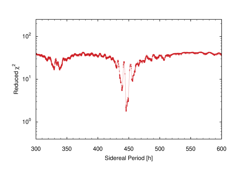
Figure 2: Result of the sidereal period scan.

In order to identify the coarse direction of the spin axis we run the optimization procedure by using the best-fit sidereal period derived in the previous paragraph as a starting value and by fixing the spin axis orientation to each of about 20,000 trial directions equally spaced on the celestial sphere. The shape of the object, the sidereal period and the photometric parameters (but not the pole coordinates) are simultaneously optimized for each trial pole. The resulting $\chi^{2}$ values for each solution are mapped on the celestial sphere via a polar azimuthal equidistant projection and are shown in Figure 3. As expected, two, equally significant loci for the best solution are identified. This is the consequence of the ambiguity theorem (Kaasalainen & Lamberg, 2006) that states that if disk-integrated photometric observations are always carried out in the same photometric plane – as is the case for low-inclination objects observed from Earth – then two indistinguishable solutions exist that satisfy the observations and that are separated by about 180$\arcdeg$ in Ecliptic longitude. The shapes corresponding to the two solutions are approximately mirrored shapes of one another around the body XY-plane. The graph also shows that both solutions are prograde and, as already inferred by Buie et al. (2018), the obliquity of the spin axis is low.

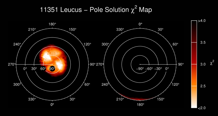
Figure 3: Polar azimuthal equidistant projection of the $\chi^{2}$ of the pole solutions. The coordinates are expressed in the J2000 Ecliptic Frame. The left panel is centered on the North Ecliptic pole and the right one on the South Ecliptic pole. The loci of the two complementary best solutions are clearly visible as white regions.

4.4 Fit to the occultation data

By providing disk-resolved information, occultation data can resolve the pole ambiguity, fix the absolute scale of the shape model and, together with the determined $H_{V}$-value, measure its geometric albedo.
In principle, occultation data can also be used to derive non-convex shape models, provided sufficient, densely sampled silhouettes are available at multiple rotation phases. Much work has been recently done concerning the optimal fusion of data coming from disk-integrated photometry and disk-resolved techniques as stellar occultations, adaptive-optics direct imaging and interferometry (e.g. Kaasalainen & Viikinkoski 2012; Viikinkoski et al. 2015). In the case of Leucus, however, both the limited lightcurve coverage and the sparse silhouette sampling would not allow a reliable non-convex model to be derived. For this reason we decided to adopt an approach similar to Durech et al. (2011) and favor the advantages of the uniqueness and stability of a convex solution.

For each of the two best candidate solutions from the previous section we project the vertices of the shape model onto the plane of sky at the time of each occultation event and then compute the 2D convex hull of the projected points. Applying this procedure to the two complementary solutions visible in Fig. 3 allowed us to unambiguously identify the correct solution as the one centered at an Ecliptic longitude of around 210$\arcdeg$. However, it also became apparent that the best solution had a slight systematic deviation in the orientation of the projection with respect to the occultation data that could be explained by a slight offset ($\approx$5$\arcdeg$) in the direction of the spin axis orientation of the model. Such a small mismatch was not unexpected, as the loci of the solutions in Fig. 3 are quite broad and shallow, and a small shift in the spin axis direction of the model would produce fits to the lightcurves with similar $\chi^{2}$. On the other hand, disk-resolved data as stellar occultations are much more sensitive to a pole misalignment. For this reason we decided to use the occultation data for the refinement of the solution.

As a goodness of fit for the occultation data we define a metric

$$\chi_{occ}^{2}=\sum\limits_{i,j}\frac{{(D_{ij})^{2}}}{N_{op}}$$ (3)

where $D_{ij}$ represents the minimum Euclidean distance between the occultation transition point $j$ (either ingress or egress) of the event $i$ and the model 2D convex hull of the event $i$. $N_{op}$ is the total number of the observed transition points. This metric is different from the one chosen by Durech et al. (2011), who prefer to use the distance of the occultation points to the occultation limb measured in the direction of the asteroid ground track. Their choice is justified by the fact that the largest contribution to their occultation data is given by timing errors and observer reaction times, which act along track. In our case, on the other hand, we estimate the largest errors to be due to the convex shape model, which are not expected to have a preferred direction.

$\chi_{occ}^{2}$ is minimized by optimizing the global scale and the Cartesian coordinates of the centers of the projections for each occultation epoch. The latter is necessary to compensate both for inaccuracies in the position of the occulted stars and for the uncertainties of the target ephemeris at the epochs of the occultations. In practice the minimization is performed by varying the projection centers and the $A_{LSL}$ albedo (see Appendix A) – which constrains the scale – in an adaptive grid search fashion.

One practical problem arises from the fact that the convex shape optimization is performed in the EGI space, while the occultation profile optimization is done in the space of the projected shape. It is therefore impractical to perform a simultaneous, combined optimization. For this reason we used the $\chi_{occ}^{2}$ as a mild penalty function for a combined $\chi_{tot}^{2}$ of the form

$$\chi_{tot}^{2}=\chi_{conv}^{2}+\lambda\chi_{occ}^{2}$$ (4)

where $\chi_{conv}^{2}$ is the term coming from the convex inversion and $\lambda$ is a small weight. The value of $\lambda$ has been determined by experimentation by adopting a value of $\lambda$ that minimized $\chi_{occ}^{2}$ without significantly increasing $\chi_{conv}^{2}$. We have then computed the quantity $\chi_{tot}^{2}$ for hundred discrete pole directions within a radius of 10$\arcdeg$ of the best solution (and of the complementary one).

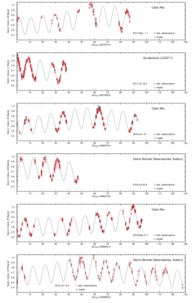
Figure 4: Observed lightcurves shown along with the respective model lightcurves. The data are plotted in intensity and are normalized to unity at the model maximum value for the respective opposition. The dates reported in the labels represent the epoch of the first observation of each sequence.

The parameters for the best-fit solution are reported in Table 2. The errors quoted for the different quantities have been determined by computing perturbed solutions and investigating the effects on the $\chi^{2}$. It must be noted that this method produces an evaluation of the statistical component of the uncertainties only. The largest contribution the errors is thought to be due to the violations of the assumptions, as the assumption of the functional form of the photometric model and the convexity assumption. Those contributions, however, are virtually impossible to be formally quantified. For this reason we refrained from using more sophisticated statistical error models, as the Markov chain Monte Carlo (MCMC) method, because they also only address the stochastic component of the uncertainty.

Figure 4 shows the synthetic lightcurves for the corresponding shape model for the epochs covered by the dense observations reported in this paper. The lightcurve intensities are corrected for changing heliocentric and topocentric range and are normalized to unity at the maximum of the respective observation window. Besides the rotational variation, the intensity variation due to the changing phase angle is visible.

Figure 5 shows the resulting best-fit model overplot onto the occultation chords by Buie et al. (2020). The complementary (wrong) solution is also plotted in light gray, showing how occultation data can help identify the correct solution. Please note that, for comparison purposes, we plot the data following Buie’s convention of projecting the shape onto the plane of sky (Green, 1985), with the $\eta$ coordinate increasing towards celestial North and the $\xi$ coordinate increasing towards East. This is a different convention than in Durech et al. (2011), who project the shape onto the fundamental plane, with the $\eta$ coordinate increasing towards West and the $\xi$ coordinate increasing towards North.

Figure 5: Occulting silhouettes of the best-fit convex model of Leucus (solid black line) along with the rejected complementary model displayed in light gray. The five panels correspond to the epochs of the five occultation events reported in (Buie et al., 2020). The red circles correspond to the starts and ends of the respective positive occultation chords. The red, green, and blue arrows represent the X, Y, and Z axes in the body-fixed reference frame, respectively. $\theta$ represents the aspect angle, i.e. the angle between the spin axis and the target-observer direction.

We note that the model shape well reproduces the occultation profiles and captures the general shape of the object, within the limits of a convex representation. In particular, it reproduces well the flat sides visible during the events LE20181118 and LE20191002 and the polygonal appearance of event LE20181118. It is also important to note that the occultation data are not directly used to derive the convex shape. The shape is influenced by the occultation data only indirectly, through the refinement of the spin axis orientation. Under this light, the match of the convex shape model to the occultation data appears even more convincing.

Figure 6: Six orthogonal projections of the best-fit Leucus convex shape arranged similarly to an unfolded dice. For contrast reasons, Lambert shading is used for the figure rendering instead of the LSL disk function used in the modeling.

Figure 6 shows six orthogonal views of the best-fit Leucus shape model. As already hinted by the occultation silhouettes, Leucus’ shape considerably deviates from an ellipsoid and is characterized by a comparatively flat Northern hemisphere.

As a sanity check, we computed the model’s inertia tensor with the method by Dobrovolskis (1996) – assuming a uniform bulk density – and established that the principal inertia axis is misaligned with respect to the body’s rotation axis by about 8$\arcdeg$. To this end, we have to recall that the derived shape model represents a convex approximation of the shape, and ignoring concavities can contribute to shift the direction of the inertia axes. Also the assumption of uniform bulk density, if violated, would contribute to shift the direction of the principal axis of inertia. The observed misalignment is therefore not necessarily a hint that the object is not in a principal rotation state. Rather, it is an expression of the fact that the convex shape represents a photometric shape, which can locally differ from the physical shape.

The maximum extent of a complex shape can be defined in several different ways (see e.g. Torppa et al. 2008). For our model we define the maximum dimensions as

$$\begin{array}[]{ccc}L_{X}=max(x_{1},...,x_{i})-min(x_{1},...,x_{i})\\ L_{Y}=max(y_{1},...,y_{i})-min(y_{1},...,y_{i})\\ L_{Z}=max(z_{1},...,z_{i})-min(z_{1},...,z_{i})\end{array}$$ (5)

where $(x_{i},y_{i},z_{i})$ represent the Cartesian coordinates of the $i^{th}$ vertex of the shape model and the $X$, $Y$, and $Z$ body axes are defined as per Sec. 4.2. This definition produces similar – but not identical – extents as the Overall Dimensions (OD) definition of Torppa et al. (2008) (see their Fig. 1). In particular, with our definition the largest extent is computed in the general direction of the principal axis of smallest inertia, which represents a natural axis of the body. In the case of the OD definition by Torppa et al. (2008), on the other hand, the maximum dimension is the largest extent that occurs anywhere in the XY plane. As an example, for a hypothetical body with a rectangular equatorial cross section, with our definition the maximum extent would be represented by the longest side of the rectangle, while, according to the definition by Torppa the maximum extent would be represented by the diagonal of the rectangle.

With our definition, the maximum dimensions for Leucus are $L_{X}=60.8$ km, $L_{Y}=39.2$ km and $L_{Z}=27.8$ km (see Table 2). Those compare with the axes (63.8, 36.6, 29.6) km of the ellipsoidal approximation by Buie et al. (2020) that were derived under the assumption of a strictly equatorial aspect during the occultation events. In the same table the orientation of the model is described both by reporting the Ecliptic J2000 coordinates of the spin axis and initial angle $\Phi_{0}$ at the epoch $T_{0}$ using the formalism by Kaasalainen et al. (2001), as well as using the IAU convention of reporting the ICRF equatorial coordinates of the spin axis and the $W_{0}$ angle at the standard epoch J2000 (Archinal et al. 2018, 2019).

The surface-equivalent spherical diameter of the convex model is $D=41.0\pm 0.7$ km, whereas its volume is $(30\pm 2)\times 10^{3}~{}\rm km^{3}$. It should be noted, however, that due to the likely presence of concavities the quoted value for the volume rather represents an upper bound.

Table 2: Results

Sidereal Period (h)	445.683 $\pm$ 0.007
Pole J2000 Ecl. Longitude ($\arcdeg$)	208
Pole J2000 Ecl. Latitude ($\arcdeg$)	+77
Pole J2000 RA ($\arcdeg$)	248
Pole J2000 Dec ($\arcdeg$)	+58
Radius of pole uncertainty ($\arcdeg$, 1$\sigma$)	3
Ecliptic obliquity of pole ($\arcdeg$)	13
Orbital obliquity of pole ($\arcdeg$)	10
$T_{0}$ (JDTDB)	2456378.0
$\Phi_{0}$ ($\rm\arcdeg$)	-76.129
$W_{0}$ ($\arcdeg$)	60.014
$\dot{W}$ ($\rm\arcdeg day^{-1}$)	19.38596 $\pm$ 0.00030
$p_{\rm V}$	0.043 $\pm$ 0.002
$A_{\rm LSL}$	0.061 $\pm$ 0.002
$A_{0}$	0.23 $\pm$ 0.09
$D$ (rad)	0.075 $\pm$ 0.015
$k$ ($\rm rad^{-1}$)	-1.07 $\pm$ 0.23
$c$ (fixed)	0.1
$H_{\rm V-LSL}$ (sph. int.)	10.979 $\pm$ 0.037
$H_{\rm V-lin}$ (sph. int.)	11.034 $\pm$ 0.035
$\beta$ ($\rm mag/\arcdeg$)	0.0395 $\pm$ 0.005
$H_{\rm V-HG}$ (sph. int.)	10.894 $\pm$ 0.004
$G$	0.34 $\pm$ 0.02
$H_{\rm V-HG_{1}G_{2}}$ (sph. int.)	10.95 $\pm$ 0.01
$G_{1}$	0.63 $\pm$ 0.04
$G_{2}$	0.23 $\pm$ 0.02
$V-R$	0.464 $\pm$ 0.015
$V-r^{\prime}$	0.313 $\pm$ 0.021
$L_{X}\rm(km)$	60.8
$L_{Y}\rm(km)$	39.2
$L_{Z}\rm(km)$	27.8
Surface-equivalent spherical diam. $\rm(km)$	41.0 $\pm$ 0.7
Photometric surface $\rm(km^{2})$	5288 $\pm$ 180
Volume $\rm(km^{3})$	$\leq 3.0\times 10^{4}$

Note. — Please refer to the text for the definition of the respective quantities.

4.5 Sphere-integrated phase curve

The disk-integrated phase curve of an object condenses the often complex parameter space of a photometric function into a two-dimensional space. As such, the phase curve is a useful phenomenological tool to compare and classify different objects, and to infer the presence of physical phenomena, as e.g. coherent backscattering. A practical difficulty in deriving phase curves, however, is that during a single apparition – and even more so across multiple apparitions – in addition to the phase angle also other viewing and illumination angles change (i.e. aspect angle and photometric obliquity), which affects the phase curves. This effect is more pronounced the more the object deviates from a sphere. Having determined through modeling the surface phase function, however, it is possible to compute the phase curve that the object would display if it were a sphere, freeing it from any dependence on the shape and thus being only the expression of the photometric properties of the surface regolith. This is achieved by integrating the surface phase function over a sphere in a range of phase angles, as detailed in Appendix A. This representation, which we refer to as the sphere-integrated phase curve corresponds to the reference phase curves defined by Kaasalainen et al. (2001) in the particular case of a sphere. Figure 7 shows the sphere-integrated phase curve for the LSL photometric function for Leucus (red line), corresponding to the best-fit photometric parameters derived in Section 4.4 and listed in Table 2. For the purpose of comparison, fits are also shown for 1) the best-fit linear phase function ($\beta=0.0395\rm mag/\arcdeg$) 2) the IAU HG system (Bowell et al., 1989) and 3) the more recently adopted IAU $\rm{HG_{1}G_{2}}$ system (Muinonen et al., 2010). .

As already apparent during the 2016 apparition (Buie et al., 2018), and as observed for several other Trojans (see e.g. Shevchenko et al. 2012), Leucus has a very subtle – if at all – opposition effect. Within the observed phase angle range, all of the phase curves except for the HG curve – that shows systematic variations both at the small and at the large end of the phase angle range – provide a good fit to the data. The extrapolation at zero phase produces $H_{\rm V-lin}$ and $H_{\rm V-HG_{1}G_{2}}$ values that differ from the LSL solution ($H_{\rm V-LSL}$) by about 0.05 mag and 0.03 mag, respectively. These small deviations are partly due to the fact that no calibrated data were available in the V band below the phase angle of about 1.6$\arcdeg$ to constrain the fit. Buie et al. (2018) did observe Leucus in the r’ band at phase angles as low as 0.125$\arcdeg$ during the 2016 apparition. However, there appear to be calibration inconsistencies between the 2016 observations and those acquired at the LCOGT in 2017 that are not fully understood. For this reason the 2016 observations were used as a relative data set .

.

It is also important to recall that since Leucus has a considerably larger equatorial cross section than the polar one, oppositions with pole-on aspect would result in measured phase curves that are brighter than the sphere-integrated phase curve and conversely, apparitions with equator-on aspect would appear fainter than the spherical model. Given the low obliquity of Leucus’ spin axis, however, all apparitions tend to be at near-equatorial aspect, as observed from Earth, and therefore Leucus never exposes its largest cross section to the observer.

Figure 7: Sphere-integrated phase curve obtained by integrating the best-fit LSL photometric function over a sphere (red solid curve). The blue squares represent the single photometric points for which absolute calibrations and transformations to the Johnson V band were available. Those data points have been corrected by multiplying the intensity of the original photometric measurement by the ratio of intensity of the spherical model to that of the best-fit convex shape model. In this way the effects of changing viewing and observing geometry, as well as the rotational variations are removed. The remaining scatter in the data is mostly due to the SNR of the measurements and to the uncertainty in the zero points of the absolute calibrations. A fit to the data by using the IAU HG system and a linear phase function are also shown for comparison.

4.6 Albedo

The geometric albedo is quite an elusive quantity to measure. First, it is defined for an observation geometry (0$\arcdeg$ solar phase angle) that is rarely observable from Earth, and in which the photometric behavior of different planetary surfaces can wildly vary. Second, it is the result of an indirect measurement that requires the brightness at zero phase and a further measurement as a thermal flux or a geometric cross section, which adds to the total error budget. Third, the albedo depends in principle on the shape of the object, although this issue is less of a problem for dark objects as the Trojans. The error on the brightness at zero phase directly translates into the same relative error for the geometric albedo (i.e. a 10$\%$ error in the brightness would cause a 10$\%$ error in the albedo). In our case the geometric albedo is derived through the simultaneous fit of the photometric lightcurves and the occultation data and by applying Eq. A3, which results in an accurate geometric albedo determination $~{}p_{\rm V}=0.043\pm 0.002$.

Grav et al. (2012) report for Leucus a much higher geometric albedo of $p_{\rm V}=0.079\pm 0.013$ and a spherical-equivalent diameter $D=34.155\pm 0.646$ km derived from WISE observations. Those values are clearly incompatible with the occultation footprints. Part of the reason for their overestimation of the albedo is that they used an inaccurate $H_{\rm V}=10.70$, retrieved from the Minor Planet Center database. Very often, those photometric measurements are acquired in non-standard photometric systems, are subject to inaccurate calibrations, and are therefore affected by large uncertainties. A further reason for the discrepancy is that the WISE observations happen to have occurred in the vicinity of the lightcurve minimum, thereby underestimating the average thermal flux of Leucus. If we use our value $H_{\rm V-LSL}=10.979$ to correct their determination by using the method proposed by Harris & Harris (1997), and account for the apparent visible cross-section at the time of the WISE observations, we obtain a corrected geometric albedo $p_{\rm V}=0.048\pm 0.014$ and a diameter $D=39\pm 1$ km. With these corrections applied, the WISE determinations are compatible with our own, within the respective uncertainties.

Figure 8: WISE observations (Grav et al., 2012) in the W3 12 $\mu$m thermal band are phased with a synthetic lightcurve from our convex model for the same epoch. Data points beyond rotational phase 1.0 are repeated for clarity. The magnitude scale for the WISE observations is arbitrarily offset to provide the best fit to the model curve. The plot shows that the WISE observations of Leucus were acquired near the lightcurve minimum.

The IRAS albedo and size determinations by Tedesco et al. (2004) (0.063$\pm{0.014}$ and 42.2$\pm{4.0}$ km, respectively) were based on an inaccurate H-value of 10.5. By using our $H_{\rm V-LSL}$ value we update their determinations to $p_{\rm V}=0.041\pm 0.014$ and $D=41.9\pm 4.0$, which are also in agreement with our own determinations.

Buie et al. (2020) determined geometric albedo values for the four occultation events in 2018 and 2019 by estimating the object cross-sectional area from best-fit ellipses and by using the absolute photometry reported in this paper. They derived geometric albedo values ranging from 0.035 to 0.043 for the different occultation events, with the scatter of the measurements probably reflecting the uncertainty in the different elliptical approximations of the occultation profiles.

5 Discussion

The combination of time-resolved, disk-integrated photometry and stellar occultations is a powerful technique that allows accurate characterization from the ground of otherwise unresolved targets. We have determined a convex shape model that is compatible with the available occultation footprints and, thanks to accurate absolute photometry, produces precise size and albedo estimates of Leucus. Our model also allows us to understand and correct previous incompatible radiometric albedo and size determinations.

The accuracy of our rotation model is such that the 1$\sigma$ uncertainty on the rotation phase will be smaller than 2$\arcdeg$ at the time of the June 2028 Lucy encounter with Leucus. At the time of the fly-by the sub-solar latitude will be about -9$\arcdeg$ and the South pole will be permanently illuminated – although at grazing incidence – whereas the North pole will be in its winter night. Unfortunately, due to the slow rotation of the body, Lucy will be able to observe at most 60$\%$ of the surface in the 40 hours during which the object will be resolved with more than 40 pixels. For this reason, an accurate ground-based shape model is very valuable to the mission. On the one hand it enables careful planning of the acquisition sequences, in order to guarantee optimum sampling. On the other hand, it complements the data from the mission to complete the uncharted hemisphere, similarly to what was done, e.g., in the case of the Rosetta fly-by of Lutetia (Carry et al., 2010; Preusker et al., 2012). The latter is of crucial importance for the estimation of the volume of the object and hence of its bulk density. Our convex model already serves this purpose well and represents a good second-order approximation of the shape – the first order being an ellipsoid (Buie et al., 2020).

With an angular size of the longest axis of 15 mas at most, Leucus represents a challenging target to resolve for ground-based adaptive optics, James Webb Space Telescope or ESO’s ALMA observations. Further improvement of the shape model in the near future can likely only come from dense stellar occultation data at further geometries, and from more, accurate absolute lightcurves. These data could be possibly used to produce a realistic non-convex model, provided the observation geometries are favorable. In this respect it is important to recall that not all concavities are directly resolvable from stellar occultations. A Star-Wars Death-Star shape, for example, would always project a convex occultation silhouette, with its concavity only being hinted at by a flat side of the contour.

Our photometric modeling of Leucus confirms that the object is very dark and lacks a pronounced opposition effect. These properties put Leucus in the context of other Trojan asteroids, and of other primitive, Outer-Belt objects. Due to the limited phase angle range achievable from Earth, however, we caution from extrapolating the derived phase curve to predict the brightness of Leucus at the large phase angles occurring on Lucy approach ($>$ 90$\arcdeg$), because it could be in error by a considerable factor. For this purpose it will be important to benefit from Lucy’s vantage point during the cruise phase to extend the coverage of the phase curve to larger angles. Such measurements would also allow the use of more sophisticated photometric models and to uniquely retrieve their parameters. Further, they would allow a reliable determination of the phase integral, which, together with the geometric albedo, is critical to establish the thermal balance of the body.

Pravec et al. (2014) revised the damping time scales for excited rotation as a function of asteroid size and rotation period. By assuming a bulk density for Leucus of $1\times 10^{3}$ kg m^-3, their estimate would translate into a relaxation time for Leucus in the range 2.3 - 3.0 Gyr. If excited rotation was ever present for Leucus it could be still in place as of today. Given the good fit of the lightcurves to our simple-rotation model, however, we conclude that if an excited rotation is present, its precession amplitude must be small. Due to the short duration of the fly-by, it is unlikely that any degree of precession can be detected by Lucy from resolved imagery. Instead, unresolved photometric sequences acquired by Lucy during the last few months of approach could be used to search for multiple periodicities in the lightcurves. The detection of a non-principal rotation state would place additional constraints on the dynamics and the internal structure of Leucus.

Appendix A Photometric quantities

For the convex shape inversion we use a photometric function defined as the product of a Lommel-Seeliger-Lambert disk function and a 3-parameter linear-exponential surface phase function (Kaasalainen et al., 2001; Schröder et al., 2013). The corresponding radiance factor ($I/F$) can be written as:

$$I/F=A_{LSL}~{}\mu_{0}\left(\frac{1}{\mu+\mu_{0}}+c\right)f(\alpha)$$ (A1)

where $A_{LSL}$ is the Lommel-Seeliger Lambert albedo, $\mu_{0}$ and $\mu$ are the incidence and emission angles, respectively, and $c$ is the weight for the Lambert contribution. The term $c$ can be either constant, or a function of the phase angle $\alpha$. In the latter case the Lommel-Seeliger Lambert disk function is equivalent to the Lunar-Lambert disk function in the formulation of McEwen (1996). The term $f$($\alpha$) is the surface phase function (expressed in intensity), which, following Kaasalainen et al. (2001) we choose to be of the form :

$$f(\alpha)=A_{0}~{}e^{-\alpha/D}+k\alpha+1$$ (A2)

where $A_{0}$ and $D$ are parameters that determine the amplitude and angular width of the exponential term, respectively, and $k$ is the slope of the linear component. The phase angle $\alpha$ is expressed in radians. With this formalism the geometric albedo for a sphere is:

$$p_{V}=A_{LSL}~{}\left(\frac{1}{2}+\frac{2}{3}c_{0}\right)(A_{0}+1)$$ (A3)

where $c_{0}$ is the value of the Lambert weight at zero phase angle.

The disk-integrated phase function for a sphere, expressed in intensity and normalized to unity at zero phase is (Li et al., 2015, 2020):

$$\Phi_{LSL}(\alpha)=\frac{[4c/(3\pi)~{}(sin(\alpha)+(\pi-\alpha)~{}cos(\alpha))+(1+sin(\alpha/2)~{}ln(tan(\alpha/4))~{}tan(\alpha/2))]}{(4c_{0}/3+1)}~{}\frac{f(\alpha)}{(A_{0}+1)}.$$ (A4)

References

- Archinal et al. (2018) Archinal, B. A., Acton, C. H., A’Hearn, M. F., et al. 2018, Celestial Mechanics and Dynamical Astronomy, 130, 22, doi: 10.1007/s10569-017-9805-5
- Archinal et al. (2019) Archinal, B. A., Acton, C. H., Conrad, A., et al. 2019, Celestial Mechanics and Dynamical Astronomy, 131, 61, doi: 10.1007/s10569-019-9925-1
- Bellm et al. (2019) Bellm, E. C., Kulkarni, S. R., Graham, M. J., et al. 2019, PASP, 131, 018002, doi: 10.1088/1538-3873/aaecbe
- Bertin & Arnouts (1996) Bertin, E., & Arnouts, S. 1996, A&AS, 117, 393, doi: 10.1051/aas:1996164
- Bowell et al. (1989) Bowell, E., Hapke, B., Domingue, D., et al. 1989, in Asteroids II, ed. R. P. Binzel, T. Gehrels, & M. S. Matthews, 524–556
- Buie et al. (2020) Buie, M. W., Keeney, B. A., Strauss, R. H., et al. 2020, current issue
- Buie et al. (2018) Buie, M. W., Zangari, A. M., Marchi, S., Levison, H. F., & Mottola, S. 2018, AJ, 155, 245, doi: 10.3847/1538-3881/aabd81
- Carry et al. (2010) Carry, B., Kaasalainen, M., Leyrat, C., et al. 2010, A&A, 523, A94, doi: 10.1051/0004-6361/201015074
- Dobrovolskis (1996) Dobrovolskis, A. R. 1996, Icarus, 124, 698, doi: 10.1006/icar.1996.0243
- Durech et al. (2010) Durech, J., Sidorin, V., & Kaasalainen, M. 2010, A&A, 513, A46, doi: 10.1051/0004-6361/200912693
- Durech et al. (2011) Durech, J., Kaasalainen, M., Herald, D., et al. 2011, Icarus, 214, 652, doi: 10.1016/j.icarus.2011.03.016
- Evans et al. (2018) Evans, D. W., Riello, M., De Angeli, F., et al. 2018, A&A, 616, A4, doi: 10.1051/0004-6361/201832756
- Flewelling et al. (2016) Flewelling, H. A., Magnier, E. A., Chambers, K. C., et al. 2016, The Pan-STARRS1 Database and Data Products. https://arxiv.org/abs/1612.05243
- French et al. (2013) French, L. M., Stephens, Robert, D., Coley, D. R., et al. 2013, Minor Planet Bulletin, 40, 198
- Gaia Collaboration et al. (2018) Gaia Collaboration, Spoto, F., Tanga, P., et al. 2018, A&A, 616, A13, doi: 10.1051/0004-6361/201832900
- Grav et al. (2012) Grav, T., Mainzer, A. K., Bauer, J. M., Masiero, J. R., & Nugent, C. R. 2012, ApJ, 759, 49, doi: 10.1088/0004-637X/759/1/49
- Green (1985) Green, R. M. 1985, Spherical Astronomy
- Hapke (2012) Hapke, B. 2012, Icarus, 221, 1079, doi: 10.1016/j.icarus.2012.10.022
- Harris (2002) Harris, A. W. 2002, Icarus, 156, 184, doi: 10.1006/icar.2001.6778
- Harris & Harris (1997) Harris, A. W., & Harris, A. W. 1997, Icarus, 126, 450, doi: 10.1006/icar.1996.5664
- Harris et al. (1984) Harris, A. W., Young, J. W., Scaltriti, F., & Zappala, V. 1984, Icarus, 57, 251, doi: 10.1016/0019-1035(84)90070-8
- Harris et al. (1989) Harris, A. W., Young, J. W., Bowell, E., et al. 1989, Icarus, 77, 171, doi: 10.1016/0019-1035(89)90015-8
- Henden et al. (2012) Henden, A. A., Levine, S. E., Terrell, D., Smith, T. C., & Welch, D. 2012, Journal of the American Association of Variable Star Observers (JAAVSO), 40, 430
- Kaasalainen & Lamberg (2006) Kaasalainen, M., & Lamberg, L. 2006, Inverse Problems, 22, 749, doi: 10.1088/0266-5611/22/3/002
- Kaasalainen et al. (2012) Kaasalainen, M., Lu, X., & Vänttinen, A. V. 2012, A&A, 539, A96, doi: 10.1051/0004-6361/201117982
- Kaasalainen et al. (2002) Kaasalainen, M., Mottola, S., & Fulchignoni, M. 2002, Asteroid Models from Disk-integrated Data, 139–150
- Kaasalainen & Torppa (2001) Kaasalainen, M., & Torppa, J. 2001, Icarus, 153, 24, doi: 10.1006/icar.2001.6673
- Kaasalainen et al. (2001) Kaasalainen, M., Torppa, J., & Muinonen, K. 2001, Icarus, 153, 37, doi: 10.1006/icar.2001.6674
- Kaasalainen & Viikinkoski (2012) Kaasalainen, M., & Viikinkoski, M. 2012, A&A, 543, A97, doi: 10.1051/0004-6361/201219267
- Kaasalainen et al. (2005) Kaasalainen, S., Kaasalainen, M., & Piironen, J. 2005, A&A, 440, 1177, doi: 10.1051/0004-6361:20053199
- Kubica et al. (2007) Kubica, J., Denneau, L., Grav, T., et al. 2007, Icarus, 189, 151, doi: 10.1016/j.icarus.2007.01.008
- Lamberg (1993) Lamberg, L. 1993, PhD thesis, University of Helsinki
- Lebedev & Laikov (1999) Lebedev, V. I., & Laikov, D. N. 1999, Doklady Mathematics, 59, 477
- Levison & Lucy Science Team (2016) Levison, H. F., & Lucy Science Team. 2016, in Lunar and Planetary Science Conference, Lunar and Planetary Science Conference, 2061
- Li et al. (2015) Li, J. Y., Helfenstein, P., Buratti, B., Takir, D., & Clark, B. E. 2015, Asteroid Photometry, 129–150, doi: 10.2458/azu_uapress_9780816532131-ch007
- Li et al. (2020) Li, J.-Y., Helfenstein, P., Buratti, B. J., Takir, D., & Clark, B. E. 2020, Icarus, 337, 113354, doi: https://doi.org/10.1016/j.icarus.2019.06.015
- McEwen (1996) McEwen, A. S. 1996, in Lunar and Planetary Science Conference, Vol. 27, Lunar and Planetary Science Conference, 841
- Minkowski (1897) Minkowski, H. 1897, Nachrichten von der Gesellschaft der Wissenschaften zu Göttingen, Mathematisch-Physikalische Klasse, 1897, 198. http://eudml.org/doc/58391
- Morbidelli et al. (2005) Morbidelli, A., Levison, H. F., Tsiganis, K., & Gomes, R. 2005, Nature, 435, 462, doi: 10.1038/nature03540
- Mottola et al. (1995) Mottola, S., De Angelis, G., Di Martino, M., et al. 1995, Icarus, 117, 62, doi: 10.1006/icar.1995.1142
- Muinonen et al. (2010) Muinonen, K., Belskaya, I. N., Cellino, A., et al. 2010, Icarus, 209, 542, doi: 10.1016/j.icarus.2010.04.003
- Nesvorný et al. (2013) Nesvorný, D., Vokrouhlický, D., & Morbidelli, A. 2013, ApJ, 768, 45, doi: 10.1088/0004-637X/768/1/45
- Oszkiewicz et al. (2012) Oszkiewicz, D. A., Bowell, E., Wasserman, L. H., et al. 2012, Icarus, 219, 283, doi: 10.1016/j.icarus.2012.02.028
- Penttilä et al. (2016) Penttilä, A., Shevchenko, V. G., Wilkman, O., & Muinonen, K. 2016, Planet. Space Sci., 123, 117, doi: 10.1016/j.pss.2015.08.010
- Pravec et al. (2014) Pravec, P., Scheirich, P., Ďurech, J., et al. 2014, Icarus, 233, 48, doi: 10.1016/j.icarus.2014.01.026
- Press et al. (1992) Press, W. H., Teukolsky, S. A., Vetterling, W. T., & Flannery, B. P. 1992, Numerical recipes in C. The art of scientific computing
- Preusker et al. (2012) Preusker, F., Scholten, F., Knollenberg, J., et al. 2012, Planet. Space Sci., 66, 54, doi: 10.1016/j.pss.2012.01.008
- Roig et al. (2008) Roig, F., Ribeiro, A. O., & Gil-Hutton, R. 2008, A&A, 483, 911, doi: 10.1051/0004-6361:20079177
- Rubincam (2000) Rubincam, D. P. 2000, Icarus, 148, 2, doi: 10.1006/icar.2000.6485
- Schröder et al. (2013) Schröder, S. E., Mottola, S., Keller, H. U., Raymond, C. A., & Russell, C. T. 2013, Planet. Space Sci., 85, 198, doi: 10.1016/j.pss.2013.06.009
- Shevchenko et al. (2012) Shevchenko, V. G., Belskaya, I. N., Slyusarev, I. G., et al. 2012, Icarus, 217, 202, doi: 10.1016/j.icarus.2011.11.001
- Shevchenko et al. (2016) Shevchenko, V. G., Belskaya, I. N., Muinonen, K., et al. 2016, Planet. Space Sci., 123, 101, doi: 10.1016/j.pss.2015.11.007
- Shoemaker et al. (1989) Shoemaker, E. M., Shoemaker, C. S., & Wolfe, R. F. 1989, in Asteroids II, ed. R. P. Binzel, T. Gehrels, & M. S. Matthews, 487–523
- Tabur (2007) Tabur, V. 2007, PASA, 24, 189, doi: 10.1071/AS07028
- Tedesco et al. (2004) Tedesco, E. F., Noah, P. V., Noah, M., & Price, S. D. 2004, NASA Planetary Data System, IRAS
- Tonry et al. (2018) Tonry, J. L., Denneau, L., Heinze, A. N., et al. 2018, PASP, 130, 064505, doi: 10.1088/1538-3873/aabadf
- Torppa et al. (2008) Torppa, J., Hentunen, V. P., Pääkkönen, P., Kehusmaa, P., & Muinonen, K. 2008, Icarus, 198, 91, doi: 10.1016/j.icarus.2008.07.014
- Viikinkoski et al. (2015) Viikinkoski, M., Kaasalainen, M., & Durech, J. 2015, A&A, 576, A8, doi: 10.1051/0004-6361/201425259
- Warner et al. (2009) Warner, B. D., Harris, A. W., & Pravec, P. 2009, Icarus, 202, 134, doi: 10.1016/j.icarus.2009.02.003
- Yoder (1979) Yoder, C. F. 1979, Icarus, 40, 341, doi: 10.1016/0019-1035(79)90024-1