Double soft current at one-loop in QCD

Abstract

We study the soft behavior of QCD amplitudes with multiple hard legs and present a compact expression for double soft gluons and double soft quarks at one-loop. The color correlation of the current basically shows a dipole structure which couples to two hard legs at one time, except for a simple abelian contribution which factorizes as products of one-loop and tree-level single soft current which couples up to three hard legs. The kinematic dependence can be expressed in terms of polylogarithms (at least up to finite terms in $\epsilon$) and the results were displayed with time-like kinematics. Analytical continuation to other kinematic configurations is then discussed where we found non-trivial crossing into ingoing states. The amplitude squared is always crossing invariant, which leads to the fact that the fully differential soft function (and the TMD soft function) is universal up to three-loop.

1 Introduction

Multi-loop scattering amplitudes are complicated functions of momenta and helicities of external states. In certain kinematical regimes, gauge theory amplitudes are constrained by more symmetries thus allow a simpler form. The typical situation is when the external momenta becoming either soft or collinear, where a gauge theory amplitude factorizes into a product of universal emission factor and lower-point amplitude. The soft and collinear behaviors of gauge theory amplitudes are of great theoretical and phenomenological interest for several reasons:

• In application of QCD, soft and collinear factorization are essential for resuming large logarithms that appears in fix order calculations Collins:1989gx ; Sterman:1995fz ; Sterman:2004pd , they also provide the theoretical basis of parton shower algorithms for Monte Carlo event generators for high-energy particle collisions Buckley:2011ms .

• Fix order calculations and subtractions rely on infrared factorization, they are essential in formulating general algorithms Catani:1996vz ; Frixione:1995ms to handle and cancel infrared singularities. The extension of these next-to-leading order (NLO) algorithms to next-to-next-to-leading order (NNLO) has been performed at last ten years to improve the theoretical accuracy of perturbative QCD predictions GehrmannDeRidder:2005cm ; Catani:2007vq ; Czakon:2010td ; Boughezal:2011jf ; Czakon:2014oma . The first step at next-to-next-to-next-to-leading order (N³LO) has been taken in the last couple of years through the complete calculation of fully inclusive Higgs production at hadron colliders, and has been making exclusive use of the soft limit expansion to obtain each component of squared real-virtual Anastasiou:2013mca ; Kilgore:2013gba , double-virtual-real Duhr:2013msa ; Li:2013lsa ; Duhr:2014nda ; Dulat:2014mda , double-real-virtual Li:2014bfa ; Anastasiou:2015yha and triple-real radiation Anastasiou:2013srw contributions.

• Soft theorems, together with some mild restrictions of locality, gauge invariance/Adler zero, are sufficient to fix (tree-level) scattering amplitude for a variety of theory Hamada:2018vrw ; Rodina:2018pcb ; Kampf:2019mcd . Thus an independent study of gauge theory soft/collinear behaviors using Wilson lines will help offer a different sight of view.

Factorization at the amplitude level for the collinear sector has been obtained in Badger:2015cxa ; DelDuca:2019ggv ; DelDuca:2020vst for both tree-level quadruple and one-loop triple splitting. In this work, we focus on the soft sector, especially on the leading power behavior of QCD amplitudes when two soft partons are emitted, from general number of hard partons. At tree level, the soft amplitude can be cast into an abelian part plus an irreducible correlation part which is a color dipole Catani:1999ss . At one loop, the amplitude receives logarithmic loop corrections, while the structure of the amplitude is similar, it is still an abelian contribution plus an non-abelian correlated contribution. The abelian contribution will be the product of two “independent” single soft emissions, with one of them gets one-loop correction. The non-abelian contribution still allows a dipole structure, as in tree-level case. Combined with known results for two loop single soft amplitude that couples up to three hard particles Dixon:2019lnw , and the tree-level triple soft emission whose irreducible three-gluon correlated emissions involve color and kinematical correlations with only one hard parton at a time Catani:2019nqv , and the pure dipole part Duhr:2013msa ; Li:2013lsa ; Li:2016ctv ; Moult:2018jzp , the picture of NNNLO soft correlation with multiple hard lines is now complete at amplitude level, which promotes a further step into performing calculations for the NNNLO soft function with multiple legs Gao:2019ojf .

The outline of the paper is as follows. In section 2, we present the definition of a soft amplitude in terms of Wilson line and review known results at tree level. In section 3 we present explicit expressions for double soft gluons and double soft quarks amplitudes in color space. In section 4 we go to explain a novel approach of calculating master integrals and later in section 5 perform analytical continuation to different relevant kinematic configurations. We have tried to present the material as elementary as possible, for readers not familiar with the formalism we have provided a detailed introduction in appendix.

2 Soft Factorization and tree level amplitude

The soft current in QCD is defined as the low-energy(soft) limit of the corresponding QCD amplitude, with the properties of universal factorization Catani:2000pi ; Catani:1999ss ; Bern:1998sc ; Bern:1999ry . It is defined to all loop orders and contains all the quantum corrections to tree-level(classical) eikonal factorization formula. The one-loop single soft factorization formula has been proved in Catani:2000pi , the main conclusion there is, in the soft limit of a single gluon with color index $a$, the $n$-point amplitude factorizes into a color operator (see in A) ${{\mbox{\boldmath$J$}}}^{a}$ acting on a $n-1$ point amplitude

$$\mathcal{M}^{a}_{n}{{\buildrel q\rightarrow 0\over{\longrightarrow}}}\,\,{\varepsilon}^{\mu}(q){{\mbox{\boldmath$J$}}}^{a}_{\mu}\cdot\mathcal{M}_{n-1}\,.$$ (1)

The generalization to multiple soft emission and to all loop orders is given in Ref Feige:2014wja ,

$$\langle a_{1},\dots,a_{n}| \mathcal{M}(q_{1},\dots,q_{n};p_{1},\dots,p_{m})\rangle|_{\{q_{1},\dots,q_{n}\}\rightarrow 0}$$

$$\,\longrightarrow\,\,{\varepsilon}^{\mu_{1}}(q_{1})\dots\varepsilon^{\mu_{n}}(q_{n}){{\mbox{\boldmath$J$}}}^{a_{1}\dots a_{n}}_{\mu_{1}\dots\mu_{n}}(q_{1},\dots,q_{n})|\mathcal{M}(p_{1},\dots,p_{m})\rangle\,.$$ (2)

The factorization formula holds at leading power in the soft limit Bauer:2001yt , setting $n_{k}=p_{k}/p_{k}^{0}$, the explicit form of the color operator is

$${\varepsilon}^{\mu_{1}}(q_{1})\dots\varepsilon^{\mu_{n}}(q_{n}){{\mbox{\boldmath$J$}}}^{a_{1}\dots a_{n}}_{\mu_{1}\dots\mu_{n}}(q_{1},\dots,q_{n}) \equiv\langle q_{1},\dots,q_{n};a_{1},\dots,a_{n}|\prod_{k=1}^{n}Y^{\dagger}_{n_{k}}(0)|\Omega\rangle\,,$$ (3)

$$Y^{\dagger}_{n}(x)\equiv P\{\exp[ig_{s}{{\mbox{\boldmath$T$}}}^{a}\int_{0}^{\infty}{n\cdot A^{a}(x+sn)e^{-\eta s}}{ds}]\}\,.$$ (4)

where $Y^{\dagger}_{n}$ corresponds to outgoing soft Wilson line and ${{\mbox{\boldmath$T$}}}^{a}$ is the color space generator Catani:2000pi , see also in appendix A, and $\eta$ is the small prescription parameter. Expanding the integral we get

$$Y^{\dagger}_{n}= \sum_{m=0}^{\infty}\frac{(ig_{s})^{m}}{m!}{\mbox{\boldmath$T$}}_{n}^{a_{m}}\dots\mbox{\boldmath$T$}_{n}^{a_{2}}{\mbox{\boldmath$T$}}_{n}^{a_{1}}\int_{0}^{\infty}ds_{1}\int_{s_{1}}^{\infty}ds_{2}\dots\int_{s_{m-1}}^{\infty}ds_{m}e^{-\eta\sum_{j}s_{j}}$$ (5)

$${\rm{T}}\left[\,n\cdot A^{a_{1}}(s_{1}n)n\cdot A^{a_{2}}(s_{2}n)\dots n\cdot A^{a_{m}}(s_{m}n)\right]+\text{permutations}\,,$$ (6)

Suppose now we have some Wilson line evaluated at space-time point $x=0$ (for simplicity we consider two of them), the expectation value between vacuum and outgoing states $\beta$ is

$$\langle\beta|Y^{\dagger}_{n_{i}}Y^{\dagger}_{n_{j}}|\Omega\rangle=\sum_{m=0}^{\infty}\frac{(ig_{s})^{m}}{m!}\prod_{i=m}^{1}{\mbox{\boldmath$T$}}_{n_{i}}^{a_{i}}\sum_{l=0}^{\infty}\frac{(ig_{s})^{l}}{l!}\prod_{j=l}^{1}{\mbox{\boldmath$T$}}_{n_{j}}^{b_{j}}\int d\vec{s}\int d\vec{t}\,\,e^{-\eta\sum_{i}s_{i}}e^{-\eta\sum_{j}t_{j}}$$ (7)

$$\times\langle\beta|\,\,{\rm{T}}\,\bigg{[}{n_{i}}\cdot A^{a_{1}}(s_{1}{n_{i}})\dots n_{i}\cdot A^{a_{m}}(s_{m}{n_{i}})\,\,n_{j}\cdot A^{b_{1}}(t_{1}n_{j})\dots n_{j}\cdot A^{b_{l}}(t_{l}n_{j})\bigg{]}|\Omega\rangle$$ (8)

$$+\text{permutations}$$ (9)

$$=\sum_{m=0}^{\infty}\frac{(ig_{s})^{m}}{m!}\prod_{i=m}^{1}{\mbox{\boldmath$T$}}_{n_{i}}^{a_{i}}\sum_{l=0}^{\infty}\frac{(ig_{s})^{l}}{l!}\prod_{j=l}^{1}{\mbox{\boldmath$T$}}_{n_{j}}^{b_{j}}\int_{k_{i}}\int_{q_{j}}\int d\vec{s}\,e^{-i(k_{1}\cdot{n_{i}}-i\eta)s_{1}}\dots e^{-i(k_{m}-i\eta)\cdot{n_{i}}s_{m}}$$ (10)

$$\times\int d\vec{t}\,e^{-i(q_{1}\cdot n_{j}-i\eta)t_{1}}\dots e^{-i(q_{l}-i\eta)\cdot n_{j}t_{l}}\bm{\mathcal{F}}\bigg{[}\langle\beta|{\rm T}\,n_{i}\cdot A^{a_{1}}(s_{1}{n_{i}})\dots n_{j}\cdot A^{b_{l}}(t_{l}n_{j})|\Omega\rangle\bigg{]}$$ (11)

$$+\text{permutations}$$ (12)

$$=\sum_{{m,l}=0}^{\infty}\frac{(g_{s})^{m+l}}{m!l!}\int_{k_{i}}\int_{q_{j}}\frac{{\mbox{\boldmath$T$}}_{n_{i}}^{a_{m}}{\mbox{\boldmath$T$}}_{n_{i}}^{a_{m-1}}\dots\mbox{\boldmath$T$}_{n_{i}}^{a_{1}}}{{n_{i}}\cdot k_{m}{n_{i}}\cdot(k_{m}+k_{m-1})\dots n_{i}\cdot\sum k_{i}}\frac{{\mbox{\boldmath$T$}}_{n_{j}}^{b_{l}}{\mbox{\boldmath$T$}}_{n_{j}}^{b_{l-1}}\dots\mbox{\boldmath$T$}_{n_{j}}^{b_{1}}}{n_{j}\cdot q_{l}n_{j}\cdot(q_{l}+q_{l-1})\dots n_{j}\cdot\sum q_{j}}$$ (13)

$$\times\bm{\mathcal{F}}\bigg{[}\langle\beta|{\rm T}\,n_{i}\cdot A^{a_{1}}(s_{1}{n_{i}})\dots n_{j}\cdot A^{b_{l}}(t_{l}n_{j})|\Omega\rangle\bigg{]}+\text{permutations}\,,$$ (14)

where above we took for short hand

$$\int d\vec{s}\equiv\int_{0}^{\infty}ds_{1}\int_{s_{1}}^{\infty}ds_{2}\dots\int_{s_{m-1}}^{\infty}ds_{m}\,,\quad\quad n_{i}\cdot(k_{m}+\dots)\rightarrow n_{i}\cdot(k_{m}+\dots)-i\eta\,.$$ (15)

In the second step of Eq. (14) we use the fact the fields along $n_{i}$ direction has space-like distance to those in the direction $n_{j}$, so we only need one time-ordering operator $\rm T$. And $\bm{\mathcal{F}}$ denotes the Fourier transformation of position space Green function into momentum space, thus the bracket equals the sum of all Feynman diagrams with incoming state corresponding to vacuum $\Omega$, outgoing lines on the mass shell corresponding to the states $\beta$, and lines off the mass shell (including propagators) corresponding to the gauge field operators $n_{i}\cdot A^{a_{1}}\dots n_{j}\cdot A^{b_{l}}$. The multiplicity of the Green functions always cancels with the factors $m!\,l!$.

To illustrate, we begin with a tree level example of double soft gluon Catani:1999ss (throughout the paper we will always take $q_{2}$ and $q_{3}$ to be soft),

$${\mbox{\boldmath$J$}}_{a_{2}a_{3}}^{\mu_{2}\mu_{3}(0)}(q_{2},q_{3})=$$

$$= \frac{1}{2}\bigg{\{}{{\mbox{\boldmath$J$}}}_{a_{2}}^{\mu_{2}(0)}(q_{2})\;,{{\mbox{\boldmath$J$}}}_{a_{3}}^{\mu_{3}(0)}(q_{3})\bigg{\}}+if_{a_{2}a_{3}a}\sum_{i}{{\mbox{\boldmath$T$}}}_{i}^{a}\bigg{\{}\frac{n_{i}^{\mu_{2}}q_{2}^{\mu_{3}}-n_{i}^{\mu_{3}}q_{3}^{\mu_{2}}}{(q_{2}\cdot q_{3})\,[n_{i}\cdot(q_{2}+q_{3})]}$$

$$-\frac{n_{i}\cdot(q_{2}-q_{3})}{2[n_{i}\cdot(q_{2}+q_{3})]}\left[\frac{n_{i}^{\mu_{2}}n_{i}^{\mu_{3}}}{(n_{i}\cdot q_{2})(n_{i}\cdot q_{3})}+\frac{g^{\mu_{2}\mu_{3}}}{q_{2}\cdot q_{3}}\right]\bigg{\}}\,,$$ (16)

where above the bracket is the anticommutator of tree level single soft current

$${{\mbox{\boldmath$J$}}}_{a}^{\mu(0)}(q)=-\sum_{i}{{\mbox{\boldmath$T$}}}^{a}_{i}\frac{n_{i}^{\mu}}{n_{i}\cdot q}\,,$$ (17)

which is the only piece that survives in an abelian theory while the color antisymmetry part is typical of non-abelian theory.

The current fulfills several properties:

• It is independent of the helicity and flavor of the massless hard parton, the only information it carries is the color charge and the direction of the hard scattered parton, the latter property is dubbed “rescaling invariance”.

• Its divergence is proportional to the total color charge of the hard partons, which is a statement of on-shell gauge invariance , see a detailed discussion in appendix A.

  $$q_{2\mu_{2}}{{\mbox{\boldmath$J$}}}_{a_{2}a_{3}}^{\mu_{2}\mu_{3}(0)}(q_{2},q_{3}) =\left(-{{\mbox{\boldmath$J$}}}_{a_{3}}^{\mu_{3}(0)}(q_{3})\;\delta_{a_{2}a}+\frac{i}{2}f_{a_{2}a_{3}a}\frac{q_{2}^{\mu_{3}}}{q_{2}\cdot q_{3}}\right)\sum_{i=1}^{n}{{\mbox{\boldmath$T$}}}_{i}^{a}\;\;,$$

  $$q_{3\mu_{3}}{{\mbox{\boldmath$J$}}}_{a_{2}a_{3}}^{\mu_{2}\mu_{3}(0)}(q_{2},q_{3}) =\left(-{{\mbox{\boldmath$J$}}}_{a_{2}}^{\mu_{2}(0)}(q_{2})\;\delta_{a_{3}a}+\frac{i}{2}f_{a_{3}a_{2}a}\frac{q_{3}^{\mu_{2}}}{q_{2}\cdot q_{3}}\right)\sum_{i=1}^{n}{{\mbox{\boldmath$T$}}}_{i}^{a}\;\;.$$ (18)

In terms of spinor helicity variables, we make the current into an amplitude, in color singlet basis $\gamma^{*}\rightarrow q\bar{q}$ it takes the following form

$$\langle i_{1}{\;\bar{\imath}}_{4}|{{\mbox{\boldmath$J$}}}_{a_{2}a_{3}}^{\mu_{2}\mu_{3}(0)}(q_{2},q_{3}){\varepsilon_{\mu_{2}}}(q_{2}){\varepsilon_{\mu_{3}}}(q_{3})|\gamma^{*}\rightarrow q{\bar{q}}\rangle\equiv\sum_{\sigma\in S_{2}}{2\,(t^{a_{\sigma(2)}}t^{a_{\sigma(3)}})^{~{}{\;\bar{\imath}}_{4}}_{i_{1}}}\mathop{\cal S}\nolimits^{\rm tree}(1_{q},\sigma(2),\sigma(3),4_{\bar{q}})$$ (19)

where above we took $q$ in leg 1 and ${\bar{q}}$ in leg 4 with fundamental color indices $i_{1}$ and ${\;\bar{\imath}}_{4}$, this convention of notation is kept all through the paper. The expression for the form factors is

$$\mathop{\cal S}\nolimits^{\rm tree}(1,2^{+},3^{+},4) =\frac{\left\langle 1\,4\right\rangle}{\left\langle 1\,2\right\rangle\left\langle 2\,3\right\rangle\left\langle 3\,4\right\rangle}\,,$$

$$\mathop{\cal S}\nolimits^{\rm tree}(1,2^{+},3^{-},4) =\frac{1}{\left\langle 1\,2\right\rangle\left[2\,4\right]+\left\langle 1\,3\right\rangle\left[3\,4\right]\,}\left(\frac{1}{s_{12}+s_{13}}\frac{\left[1\,4\right]\left\langle 1\,3\right\rangle^{3}}{\left\langle 2\,3\right\rangle\left\langle 1\,2\right\rangle}+\frac{1}{s_{24}+s_{34}}\frac{\left\langle 1\,4\right\rangle\left[2\,4\right]^{3}}{\left[2\,3\right]\left[3\,4\right]}\right)\,.$$ (20)

Other color and helicity coefficients in Eq. (19) can be obtained by exchanging in Eq. (20) legs 1 and 4 or by complex conjugation, for example

$$\mathop{\cal S}\nolimits^{\rm tree}(1,3^{-},2^{+},4)=\mathop{\cal S}\nolimits^{\rm tree}(4,2^{+},3^{-},1)\,,\quad\quad\mathop{\cal S}\nolimits^{\rm tree}(1,2^{-},3^{+},4)=\mathop{\cal S}\nolimits^{\rm tree}(1,2^{+},3^{-},4)^{*}\,.$$ (21)

Likewise, we present the results for double soft quarks $Q\bar{Q}$ at tree level

$$({{\mbox{\boldmath$J$}}}^{(0)})_{i_{2}}^{~{}{\;\bar{\imath}}_{3}}(q_{2},q_{3})\equiv\sum_{n}\frac{\ooalign{$\hfil/\hfil$\crcr$n$}}{n\cdot(q_{2}+q_{3})}\frac{1}{s_{23}}(t^{d})^{~{}{\;\bar{\imath}}_{3}}_{i_{2}}{\mbox{\boldmath$T$}}_{n}^{d}\,,$$ (24)

where above $t^{d}$ is the color matrix in fundamental representation, and $i_{2}$ ${\;\bar{\imath}}_{3}$ are color indices for $Q$ and $\bar{Q}$ respectively. Taking again the color singlet basis $\gamma^{*}\rightarrow q\bar{q}$

$$\langle i_{1}{\;\bar{\imath}}_{4}|\bar{u}(q_{3})({{\mbox{\boldmath$J$}}}^{(0)})_{i_{2}}^{~{}{\;\bar{\imath}}_{3}}(q_{2},q_{3})v(q_{2})|\gamma^{*}\rightarrow q{\bar{q}}\rangle\equiv 2\,(t^{d})^{~{}{\;\bar{\imath}}_{4}}_{i_{1}}(t^{d})^{~{}{\;\bar{\imath}}_{3}}_{i_{2}}\mathop{\cal S}\nolimits^{{\rm tree}}(2\bar{Q}^{+},3Q^{-})\,,$$ (25)

$$\mathop{\cal S}\nolimits^{{\rm tree}}(2\bar{Q}^{+},3Q^{-})=\frac{1}{s_{23}}\Bigg{(}\frac{\left\langle 3\,1\right\rangle\left[1\,2\right]}{s_{12}+s_{13}}-\frac{\left\langle 3\,4\right\rangle\left[4\,2\right]}{s_{24}+s_{34}}\Bigg{)}\,.$$ (26)

3 Double soft current at one-loop

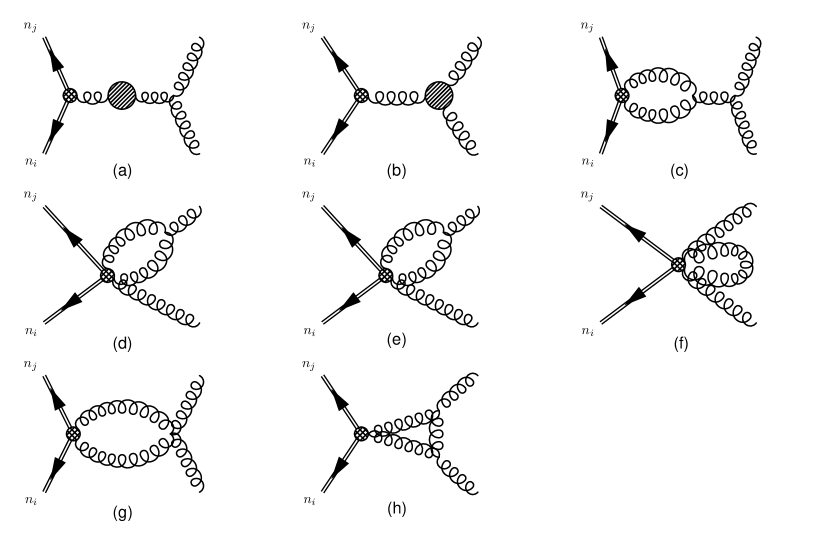
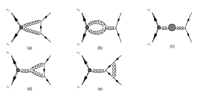
Figure 1: Non-vanishing diagrams for double soft gluons and quarks in Feynman gauge. Diagram 4 and 5 can couple to three Wilson lines, but this contribution factorizes into the abelian part.

Going beyond tree level, the soft amplitude receives quantum corrections. The single soft amplitude was first obtained in Ref. Bern:1995ix for color-ordered amplitudes, and was later re-derived in color space Catani:2000pi in axial gauge using Catani-Grazzini soft insertion rules, see also in Bern:1999ry ; Bern:1998sc ; Dixon:2019lnw .

For double soft emissions, the presence of sub-leading color structures result in an even deeper entanglement of color and kinematics. Historical treatment in the 1990s have made exclusive use of ‘primitive amplitudes’, which served as an starting point for a clean factorization of one-loop amplitudes in the soft and collinear regions by separating color issues from the kinematic issues  Bern:1998sc ; Bern:1999ry . A typical example of primitive amplitude decomposition can be found in the artwork of helicity amplitudes for $\gamma*\rightarrow 4$ partons Bern:1997sc ; Bern:1996ka , from there in principle the explicit expression for double soft emissions could be subtracted out (as we have done), but the procedure is tedious due to presence of momenta conservation in the helicity form and due to nonlinear relation of Schouten identity. Thus a direct calculation in color space is desired, we will show the details below.

3.1 Setups

Expanding both sides of Eq. (2) to one loop order in terms of bare strong coupling for double soft emission, the resulting formula becomes our starting point of the calculations

$$\langle a_{2},a_{3}|\mathcal{M}^{(1)}{(q_{2},q_{3};p_{1},\dots,p_{m})}\rangle|_{q_{2}\rightarrow 0,q_{3}\rightarrow 0}={\varepsilon}^{\mu_{2}}(q_{2}){\varepsilon}^{\mu_{3}}(q_{3})g_{s}^{2}$$

$$\times\left[{{\mbox{\boldmath$J$}}}^{a_{2}a_{3}(0)}_{\mu_{2}\mu_{3}}(q_{2},q_{3})|\mathcal{M}^{(1)}{(p_{1},\dots,p_{m})}\rangle+\bar{a}\,{{\mbox{\boldmath$J$}}}^{a_{2}a_{3}(1)}_{\mu_{2}\mu_{3}}(q_{2},q_{3})|\mathcal{M}^{(0)}{(p_{1},\dots,p_{m})}\rangle\right]\,,$$ (27)

where above the tree level current is in Eq. (16), and we have factored out a tree level normalization of $g_{s}^{2}$ for the soft current, and expanded the results in terms of rescaled coupling

$$\bar{a}\equiv\frac{g_{s}^{2}\mu^{-2\epsilon}}{(4\pi)^{2-\epsilon}}e^{-\epsilon\gamma_{E}}=\frac{\alpha_{s}}{4\pi}\frac{\mu^{-2\epsilon}e^{-\epsilon\gamma_{E}}}{(4\pi)^{-\epsilon}}\,,$$ (28)

where $\alpha_{s}=g_{s}^{2}/(4\pi)$, and $\gamma_{E}=0.577216$ is the Euler-Mascheroni constant.

We have adopted a diagram calculation approach with Feynman diagrams (see Figure 1) generated by Qgraph Nogueira:1991ex . The color/Dirac algebra and integrand manipulations were performed in form Ruijl:2017dtg . To keep track of regularization scheme dependence we set regularization-dependent dimension to be $4-2\delta_{R}\epsilon$, with $\delta_{R}=0$ referring to Four Dimensional Helicity scheme ($\rm FDH$) Bern:1991aq ; Bern:2002zk and $\delta_{R}=1$ referring to ’t Hooft-Veltman scheme ($\rm HV$) tHooft:1972tcz . The $d$-dimension loop reduction was based on IBP identities Chetyrkin:1981qh implemented in the Mathematica package LiteRed Lee:2012cn .

Below we present the expressions of the soft amplitude, with a normalization factor of

$$c_{\Gamma}\equiv{\Gamma(1+\epsilon)\Gamma^{2}(1-\epsilon)\over\Gamma(1-2\epsilon)}\,.$$ (29)

We will first work in time-like kinematic regions ($s_{ij}>0$) and later consider analytical continuations.

3.2 Time-Like results for double soft gluons

For double soft gluons, we cast the amplitudes into 2 independent helicity configurations (other helicity configuration can be achieved by complex conjugation). Just like in tree level case Eq. (16), the amplitude was further decomposed into an abelian part and a correlated emission part (non-abelain)

$${\varepsilon}_{\mu_{2}}(q_{2}){\varepsilon}_{\mu_{3}}(q_{3}){\mbox{\boldmath$J$}}_{a_{2}a_{3}}^{\mu_{2}\mu_{3}(1)}(q_{2},q_{3})=\mathcal{M}_{a_{2}a_{3}}^{\text{ab.}}(2,3)+\mathcal{M}_{a_{2}a_{3}}^{\rm{nab.}}(2,3).$$ (30)

The abelian part is a direct product of a one-loop single soft and tree-level single soft emission.

$$\Delta^{\mu}(i,j;q;\epsilon)\equiv {{\Gamma(1-\epsilon)\Gamma(1+\epsilon)}\over{\epsilon}^{2}}\Bigg{(}{\mu^{2}(-s_{ij}-i\eta)\over{(-s_{iq}-i\eta)\,\,(-s_{qj}-i\eta)\,}}\Bigg{)}^{\epsilon}\left(\frac{n_{i}^{\mu}}{n_{i}\cdot q}-\frac{n_{j}^{\mu}}{n_{j}\cdot q}\right)\,,$$ (31)

$$\,\mathcal{M}_{a_{2}a_{3}}^{\rm{ab.}}(2^{+},3^{+})= \sum_{i\neq j}^{m}if_{a_{2}cd}{\mbox{\boldmath$T$}}^{c}_{i}{\mbox{\boldmath$T$}}^{d}_{j}\Delta^{\mu_{2}}(i,j;q_{2};\epsilon){\varepsilon}_{\mu_{2}}(q_{2})\sum_{k}^{m}\frac{-n_{k}\cdot{\varepsilon}(q_{3})}{n_{k}\cdot q_{3}}{\mbox{\boldmath$T$}}_{k}^{a_{3}}+2\longleftrightarrow 3\,.$$ (32)

$$\mathcal{M}_{a_{2}a_{3}}^{\rm{nab.}}(2^{+},3^{+})=-4{\left(\frac{-s_{23}-i\eta}{\mu^{2}}\right)^{-\epsilon}}\sum_{i\neq j}^{m}f_{bca_{2}}f_{bda_{3}}{\mbox{\boldmath$T$}}^{c}_{i}{\mbox{\boldmath$T$}}^{d}_{j}{\left\langle i\,j\right\rangle\over\left\langle i\,2\right\rangle\left\langle 2\,3\right\rangle\left\langle 3\,j\right\rangle}$$ (33)

$$\times\Bigg{\{}{-2\over\epsilon^{2}}-{1\over\epsilon}\ln{s_{ij}s_{23}\over s_{i2}s_{3j}}-{1\over 2}\Bigg{(}\ln^{2}{s_{ij}s_{23}\over(s_{i2}+s_{i3})(s_{2j}+s_{3j})}+\ln^{2}{s_{i2}\over s_{i2}+s_{i3}}+\ln^{2}{s_{3j}\over s_{2j}+s_{3j}}\Bigg{)}\,$$ (34)

$$-\text{Li}_{2}(1-{s_{i2}\over s_{i2}+s_{i3}})-\text{Li}_{2}(1-{s_{3j}\over s_{2j}+s_{3j}})-\text{Li}_{2}(1-{s_{ij}s_{23}\over(s_{i2}+s_{i3})(s_{2j}+s_{3j})})\Bigg{\}}$$ (35)

$$-{\left(\frac{-s_{23}-i\eta}{\mu^{2}}\right)^{-\epsilon}}\Bigg{\{}{\frac{C_{A}-n_{f}-C_{A}\delta_{R}\epsilon}{(-1+\epsilon)(-3+2\epsilon)(-1+2\epsilon)}}\sum_{i}^{m}if_{ba_{2}a_{3}}{\mbox{\boldmath$T$}}_{i}^{b}\,{\frac{s_{i2}-s_{i3}}{s_{i2}+s_{i3}}}\frac{-1}{\left\langle 2\,3\right\rangle^{2}}\Bigg{\}}\,,$$ (36)

$$\mathcal{M}_{a_{2}a_{3}}^{\rm{nab.}}(2^{+},3^{-})=-4{\left(\frac{-s_{23}-i\eta}{\mu^{2}}\right)^{-\epsilon}}\sum_{i\neq j}^{m}f_{bca_{2}}f_{bda_{3}}{\mbox{\boldmath$T$}}^{c}_{i}{\mbox{\boldmath$T$}}^{d}_{j}$$ (37)

$$\times\Bigg{\{}{{1\over\left\langle i\,2\right\rangle\left[2\,j\right]+\left\langle i\,3\right\rangle\left[3\,j\right]\,}\left({1\over s_{i2}+s_{i3}}{\left[i\,j\right]\left\langle i\,3\right\rangle^{3}\over\left\langle 2\,3\right\rangle\left\langle i\,2\right\rangle}+{1\over s_{2j}+s_{3j}}{\left\langle i\,j\right\rangle\left[2\,j\right]^{3}\over\left[2\,3\right]\left[3\,j\right]}\right)}$$ (38)

$$\times\Bigg{(}{-2\over\epsilon^{2}}-{1\over\epsilon}\ln{s_{ij}s_{23}\over s_{i2}s_{3j}}+{1\over 2}\ln^{2}{s_{ij}s_{23}\over s_{i2}s_{3j}}-{\pi^{2}\over 3}\Bigg{)}$$ (39)

$$+{\left\langle i\,j\right\rangle\over\left\langle i\,2\right\rangle\left\langle 2\,j\right\rangle}{\left[i\,j\right]\over\left[i\,3\right]\left[3\,j\right]}\times\left({1\over 2}\ln^{2}{s_{ij}s_{23}\over s_{i2}s_{3j}}\right)$$ (40)

$$+{1\over s_{i2}+s_{i3}}\Bigg{(}{-1\over\left\langle i\,2\right\rangle\left[2\,j\right]+\left\langle i\,3\right\rangle\left[3\,j\right]\,}{\left[i\,j\right]\left\langle i\,3\right\rangle^{3}\over\left\langle 2\,3\right\rangle\left\langle i\,2\right\rangle}+{-1\over\left[i\,2\right]\left\langle 2\,j\right\rangle+\left[i\,3\right]\left\langle 3\,j\right\rangle\,}{\left\langle i\,j\right\rangle\left[i\,2\right]^{3}\over\left[2\,3\right]\left[i\,3\right]}\Bigg{)}$$ (41)

$$\times\Bigg{(}{1\over 2}\ln^{2}{s_{i2}\over s_{i2}+s_{i3}}+{1\over 2}\ln^{2}{s_{ij}s_{23}\over(s_{i2}+s_{i3})s_{3j}}\Bigg{)}$$ (42)

$$+{1\over s_{2j}+s_{3j}}\Bigg{(}{-1\over\left\langle i\,2\right\rangle\left[2\,j\right]+\left\langle i\,3\right\rangle\left[3\,j\right]\,}{\left\langle i\,j\right\rangle\left[2\,j\right]^{3}\over\left[2\,3\right]\left[3\,j\right]}+{-1\over\left[i\,2\right]\left\langle 2\,j\right\rangle+\left[i\,3\right]\left\langle 3\,j\right\rangle\,}{\left[i\,j\right]\left\langle 3\,j\right\rangle^{3}\over\left\langle 2\,3\right\rangle\left\langle 2\,j\right\rangle}\Bigg{)}$$ (43)

$$\times\Bigg{(}{1\over 2}\ln^{2}{s_{3j}\over s_{2j}+s_{3j}}+{1\over 2}\ln^{2}{s_{ij}s_{23}\over(s_{2j}+s_{3j})s_{i2}}\,\Bigg{)}\Bigg{\}}\,,$$ (44)

$$\mathcal{M}_{a_{2}a_{3}}^{\rm{nab.}}(2^{+},3^{+},2\ll 3)=4\sum_{i\neq j}^{m}f_{bca_{2}}f_{bda_{3}}{\mbox{\boldmath$T$}}^{c}_{i}{\mbox{\boldmath$T$}}^{d}_{j}{\left\langle i\,3\right\rangle\over\left\langle i\,2\right\rangle\left\langle 2\,3\right\rangle}{\left\langle i\,j\right\rangle\over\left\langle i\,3\right\rangle\left\langle 3\,j\right\rangle}\,$$ (45)

$$\Bigg{[}\Bigg{(}{1\over\epsilon^{2}}+{1\over\epsilon}\ln{-s_{i3}\,\mu^{2}\over s_{i2}\,s_{23}}+{1\over 2}\ln^{2}{-s_{i3}\,\mu^{2}\over s_{i2}\,s_{23}}+{\pi^{2}\over 6}\Bigg{)}+\Bigg{(}{1\over\epsilon^{2}}+{1\over\epsilon}\ln{-s_{ij}\,\mu^{2}\over s_{i3}\,s_{3j}}+{1\over 2}\ln^{2}{-s_{ij}\,\mu^{2}\over s_{i3}\,s_{3j}}+{\pi^{2}\over 6}\Bigg{)}\Bigg{]}\,,$$ (46)

$$\mathcal{M}_{a_{2}a_{3}}^{\rm{nab.}}(2^{+},3^{-},2\ll 3)=4\sum_{i\neq j}^{m}f_{bca_{2}}f_{bda_{3}}{\mbox{\boldmath$T$}}^{c}_{i}{\mbox{\boldmath$T$}}^{d}_{j}{\left\langle i\,3\right\rangle\over\left\langle i\,2\right\rangle\left\langle 2\,3\right\rangle}{-\left[i\,j\right]\over\left[i\,3\right]\left[3\,j\right]}\,$$ (47)

$$\Bigg{[}\Bigg{(}{1\over\epsilon^{2}}+{1\over\epsilon}\ln{-s_{i3}\,\mu^{2}\over s_{i2}\,s_{23}}+{1\over 2}\ln^{2}{-s_{i3}\,\mu^{2}\over s_{i2}\,s_{23}}+{\pi^{2}\over 6}\Bigg{)}+\Bigg{(}{1\over\epsilon^{2}}+{1\over\epsilon}\ln{-s_{ij}\,\mu^{2}\over s_{i3}\,s_{3j}}+{1\over 2}\ln^{2}{-s_{ij}\,\mu^{2}\over s_{i3}\,s_{3j}}+{\pi^{2}\over 6}\Bigg{)}\Bigg{]}\,.$$ (48)

A particular application of our result is to take the strong-ordered limit of the emitted soft gluons, the resulted expressions, as was collected in Eq. (45), can be deduced from a first principle computation.

We have taken the strong-ordered limit to be $q_{2}\ll q_{3}$, the resulted strong-ordered double soft gluon current is obtained by successive application of the single soft factorization formula Eq. (1) :

$$\langle a_{2}\,a_{3}|\mathcal{M}\rangle\rightarrow\langle a_{3}|{\mbox{\boldmath$\tilde{J}$}}^{a_{2}}_{\mu_{2}}|\mathcal{M}\rangle=\langle a_{3}|{\mbox{\boldmath$\tilde{J}$}}^{a_{2}}_{\mu_{2}}|a\rangle\langle a|\mathcal{M}\rangle\rightarrow\langle a_{3}|{\mbox{\boldmath$\tilde{J}$}}^{a_{2}}_{\mu_{2}}|a\rangle{\mbox{\boldmath$J$}}^{a}_{\mu_{3}}|\mathcal{M}\rangle\,.$$ (50)

The strong-ordered double soft gluon current is then

$${\mbox{\boldmath$J$}}_{a_{2}a_{3}}^{\mu_{2}\mu_{3}}(q_{2}\ll q_{3})=\langle a_{3}|{\mbox{\boldmath$\tilde{J}$}}^{a_{2}}_{\mu_{2}}|a\rangle{\mbox{\boldmath$J$}}^{a}_{\mu_{3}}\,.$$ (51)

The current ${\mbox{\boldmath$\tilde{J}$}}^{a_{2}}_{\mu_{2}}$ acts as an operator in the color space of ‘soft gluon $3$ + hard partons’, and the current $\langle a_{3}|{\mbox{\boldmath$\tilde{J}$}}^{a_{2}}_{\mu_{2}}|a\rangle$ is partially contracted in the color indices of soft gluon $3$ and thus acting as an operator in the space of the hard partons, making its multiplication with current ${\mbox{\boldmath$J$}}^{a}_{\mu_{3}}$ legal. It can be written as

$$\langle a_{3}|{\mbox{\boldmath$\tilde{J}$}}^{a_{2}}_{\mu_{2}}|a\rangle={\mbox{\boldmath$J$}}^{a_{2}}_{\mu_{2}}\langle a_{3}|a\rangle+\Delta{\mbox{\boldmath$J$}}^{a;a_{2},a_{3}}_{\mu_{2}}={\mbox{\boldmath$J$}}^{a_{2}}_{\mu_{2}}\delta_{a_{3}a}+\Delta{\mbox{\boldmath$J$}}^{a;a_{2},a_{3}}_{\mu_{2}}\,,$$ (52)

where the current ${\mbox{\boldmath$J$}}^{a_{2}}_{\mu_{2}}$ is the normal single soft current and $\Delta{\mbox{\boldmath$J$}}^{a;a_{2},a_{3}}_{\mu_{2}}$ incorporates nontrivial effects of color correlation with soft gluon $3$.

The tree level expression is already obtained in Catani:1999ss :

$${\mbox{\boldmath$J$}}_{a_{2}a_{3}}^{(0)\mu_{2}\mu_{3}}(q_{2}\ll q_{3})= \left({\mbox{\boldmath$J$}}^{(0)a_{2}}_{\mu_{2}}\langle a_{3}|a\rangle+\langle a_{3}|T_{3}^{a_{2}}|a\rangle\frac{q_{3\mu_{2}}}{-q_{3}\cdot q_{2}}\right){\mbox{\boldmath$J$}}^{(0)a}_{\mu_{3}}$$ (53)

$$\,= \left({\mbox{\boldmath$J$}}^{(0)a_{2}}_{\mu_{2}}\delta_{a_{3}a}+if_{a_{3}a_{2}a}\frac{q_{3\mu_{2}}}{-q_{3}\cdot q_{2}}\right){\mbox{\boldmath$J$}}^{(0)a}_{\mu_{3}}\,,$$ (54)

$$\,\Delta{\mbox{\boldmath$J$}}^{(0)a;a_{2},a_{3}}_{\mu_{2}}= if_{a_{3}a_{2}a}\frac{q_{3\mu_{2}}}{-q_{3}\cdot q_{2}}\,.$$ (55)

The one-loop expression needs a little bit effort, expanding Eq. (51) to one-loop order we get

$${\mbox{\boldmath$J$}}^{(1)a_{2}a_{3}}_{\mu_{2}\mu_{3}}(q_{2}\ll q_{3})= \langle a_{3}|{\mbox{\boldmath$\tilde{J}$}}^{(0)a_{2}}_{\mu_{2}}|a\rangle{\mbox{\boldmath$J$}}^{(1)a}_{\mu_{3}}+\langle a_{3}|{\mbox{\boldmath$\tilde{J}$}}^{(1)a_{2}}_{\mu_{2}}|a\rangle{\mbox{\boldmath$J$}}^{(0)a}_{\mu_{3}}$$ (56)

$$\,= \left[{\mbox{\boldmath$J$}}^{(0)a_{2}}_{\mu_{2}}\delta_{a_{3}a}+\Delta{\mbox{\boldmath$J$}}^{(0)a;a_{2},a_{3}}_{\mu_{2}}\right]{\mbox{\boldmath$J$}}^{(1)a}_{\mu_{3}}+\left[{\mbox{\boldmath$J$}}^{(1)a_{2}}_{\mu_{2}}\delta_{a_{3}a}+\Delta{\mbox{\boldmath$J$}}^{(1)a;a_{2},a_{3}}_{\mu_{2}}\right]{\mbox{\boldmath$J$}}^{(0)a}_{\mu_{3}}$$ (57)

$$\,= {\mbox{\boldmath$J$}}^{(0)a_{2}}_{\mu_{2}}{\mbox{\boldmath$J$}}^{(1)a_{3}}_{\mu_{3}}+{\mbox{\boldmath$J$}}^{(1)a_{2}}_{\mu_{2}}{\mbox{\boldmath$J$}}^{(0)a_{3}}_{\mu_{3}}+\Delta{\mbox{\boldmath$J$}}^{(0)a;a_{2},a_{3}}_{\mu_{2}}{\mbox{\boldmath$J$}}^{(1)a}_{\mu_{3}}+\Delta{\mbox{\boldmath$J$}}^{(1)a;a_{2},a_{3}}_{\mu_{2}}{\mbox{\boldmath$J$}}^{(0)a}_{\mu_{3}}$$ (58)

$$\,= \bigg{\{}{\mbox{\boldmath$J$}}^{(1)a_{3}}_{\mu_{3}}{\mbox{\boldmath$J$}}^{(0)a_{2}}_{\mu_{2}}+{\mbox{\boldmath$J$}}^{(1)a_{2}}_{\mu_{2}}{\mbox{\boldmath$J$}}^{(0)a_{3}}_{\mu_{3}}\bigg{\}}+\bigg{\{}\left[{\mbox{\boldmath$J$}}^{(0)a_{2}}_{\mu_{2}},{\mbox{\boldmath$J$}}^{(1)a_{3}}_{\mu_{3}}\right]+\Delta{\mbox{\boldmath$J$}}^{(0)a;a_{2},a_{3}}_{\mu_{2}}{\mbox{\boldmath$J$}}^{(1)a}_{\mu_{3}}\bigg{\}}$$ (59)

$$\,+ \Delta{\mbox{\boldmath$J$}}^{(1)a;a_{2},a_{3}}_{\mu_{2}}{\mbox{\boldmath$J$}}^{(0)a}_{\mu_{3}}\,.$$ (60)

The current receives three independent contributions, the first bracket denotes an abelian contribution. The remaining contributions are intrinsically non-abelian, and are gauge invariant on their own :

$$q_{2}^{\mu_{2}}\Delta{\mbox{\boldmath$J$}}^{(1)a;a_{2},a_{3}}_{\mu_{2}}{\mbox{\boldmath$J$}}^{(0)a}_{\mu_{3}}\simeq 0\,,\quad\quad q_{2}^{\mu_{2}}\left(\left[{\mbox{\boldmath$J$}}^{(0)a_{2}}_{\mu_{2}},{\mbox{\boldmath$J$}}^{(1)a_{3}}_{\mu_{3}}\right]+\Delta{\mbox{\boldmath$J$}}^{(0)a;a_{2},a_{3}}_{\mu_{2}}{\mbox{\boldmath$J$}}^{(1)a}_{\mu_{3}}\right)\simeq 0\,.$$ (61)

The first contribution is

$$\Delta{\mbox{\boldmath$J$}}^{(1)a;a_{2},a_{3}}_{\mu_{2}}{\mbox{\boldmath$J$}}^{(0)a}_{\mu_{3}}= 2\sum_{i=1}^{m}if_{a_{2}cd}\langle a_{3}|{\mbox{\boldmath$T$}}_{3}^{c}|a\rangle{\mbox{\boldmath$T$}}_{i}^{d}\Delta_{\mu_{2}}(3,i;q_{2};\epsilon)\sum_{j=1}^{m}\frac{-{n_{j}}_{\mu_{3}}}{n_{j}\cdot q_{3}}{\mbox{\boldmath$T$}}_{j}^{a}$$ (62)

$$\,= -2\sum_{i=1}^{m}f_{a_{2}cd}f_{a_{3}ca}{\mbox{\boldmath$T$}}_{i}^{d}\Delta_{\mu_{2}}(3,i;q_{2};\epsilon)\sum_{j=1}^{m}\left(\frac{{n_{i}}_{\mu_{3}}}{n_{i}\cdot q_{3}}-\frac{{n_{j}}_{\mu_{3}}}{n_{j}\cdot q_{3}}\right){\mbox{\boldmath$T$}}_{j}^{a}$$ (63)

$$\,= 2\sum_{i\neq j}^{m}f_{bca_{2}}f_{bda_{3}}{\mbox{\boldmath$T$}}_{i}^{c}{\mbox{\boldmath$T$}}_{j}^{d}\Delta_{\mu_{2}}(i,3;q_{2};\epsilon)\left(\frac{{n_{i}}_{\mu_{3}}}{n_{i}\cdot q_{3}}-\frac{{n_{j}}_{\mu_{3}}}{n_{j}\cdot q_{3}}\right)\,.$$ (64)

The bracket of the second contribution is

$$\left[{\mbox{\boldmath$J$}}^{(0)a_{2}}_{\mu_{2}},{\mbox{\boldmath$J$}}^{(1)a_{3}}_{\mu_{3}}\right]= \sum_{k}^{m}\sum_{i\neq j}^{m}\frac{-{n_{k}}_{\mu_{2}}}{n_{k}\cdot q_{2}}if_{a_{3}cd}\Delta_{\mu_{3}}(i,j;q_{3};\epsilon)\left[{\mbox{\boldmath$T$}}_{k}^{a_{2}},{\mbox{\boldmath$T$}}_{i}^{c}{\mbox{\boldmath$T$}}_{j}^{d}\right]$$ (65)

$$\,= \sum_{k}^{m}\sum_{i\neq j}^{m}\frac{-{n_{k}}_{\mu_{2}}}{n_{k}\cdot q_{2}}if_{a_{3}cd}\Delta_{\mu_{3}}(i,j;q_{3};\epsilon)\times\left(if_{a_{2}ce}{\mbox{\boldmath$T$}}_{k}^{e}{\mbox{\boldmath$T$}}_{j}^{d}\delta_{ki}+if_{a_{2}de}{\mbox{\boldmath$T$}}_{i}^{c}{\mbox{\boldmath$T$}}_{k}^{e}\delta_{kj}\right)$$ (66)

$$\,= -2\sum_{i\neq j}^{m}f_{bca_{2}}f_{bda_{3}}{\mbox{\boldmath$T$}}_{i}^{c}{\mbox{\boldmath$T$}}_{j}^{d}\Delta_{\mu_{3}}(i,j;q_{3};\epsilon)\frac{-{n_{i}}_{\mu_{2}}}{n_{i}\cdot q_{2}}\,.$$ (67)

The overall second contribution is then

$$\left[{\mbox{\boldmath$J$}}^{(0)a_{2}}_{\mu_{2}},{\mbox{\boldmath$J$}}^{(1)a_{3}}_{\mu_{3}}\right]+\Delta{\mbox{\boldmath$J$}}^{(0)a;a_{2},a_{3}}_{\mu_{2}}{\mbox{\boldmath$J$}}^{(1)a}_{\mu_{3}}= -2\sum_{i\neq j}^{m}f_{bca_{2}}f_{bda_{3}}{\mbox{\boldmath$T$}}_{i}^{c}{\mbox{\boldmath$T$}}_{j}^{d}\Delta_{\mu_{3}}(i,j;q_{3};\epsilon)\frac{-{n_{i}}_{\mu_{2}}}{n_{i}\cdot q_{2}}$$ (68)

$$\,+ \sum_{i\neq j}^{m}f_{a_{3}a_{2}a}f_{acd}{\mbox{\boldmath$T$}}_{i}^{c}{\mbox{\boldmath$T$}}_{j}^{d}\Delta_{\mu_{3}}(i,j;q_{3};\epsilon)\frac{{q_{3}}_{\mu_{2}}}{q_{3}\cdot q_{2}}$$ (69)

$$\,= 2\sum_{i\neq j}^{m}f_{bca_{2}}f_{bda_{3}}{\mbox{\boldmath$T$}}_{i}^{c}{\mbox{\boldmath$T$}}_{j}^{d}\Delta_{\mu_{3}}(i,j;q_{3};\epsilon)\left(\frac{{n_{i}}_{\mu_{2}}}{n_{i}\cdot q_{2}}-\frac{{q_{3}}_{\mu_{2}}}{q_{3}\cdot q_{2}}\right)\,,$$ (70)

where in the last step we have used the identity :

$$\sum_{i\neq j}^{m}(f_{bca_{2}}f_{bda_{3}}+f_{bca_{3}}f_{bda_{2}}){\mbox{\boldmath$T$}}_{i}^{c}{\mbox{\boldmath$T$}}_{j}^{d}\Delta_{\mu_{3}}(i,j;q_{3};\epsilon)=0\,.$$ (72)

Adding Eq. (64) and Eq. (LABEL:eq:2contri) we arrive at

$${\mbox{\boldmath$J$}}^{(1)a_{2}a_{3}}_{\mu_{2}\mu_{3}}(q_{2} \ll q_{3})|_{\rm{nab.}}=2\sum_{i\neq j}^{m}f_{bca_{2}}f_{bda_{3}}{\mbox{\boldmath$T$}}_{i}^{c}{\mbox{\boldmath$T$}}_{j}^{d}\left(\frac{{n_{i}}_{\mu_{2}}}{n_{i}\cdot q_{2}}-\frac{{q_{3}}_{\mu_{2}}}{q_{3}\cdot q_{2}}\right)\times\left(\frac{{n_{i}}_{\mu_{3}}}{n_{i}\cdot q_{3}}-\frac{{n_{j}}_{\mu_{3}}}{n_{j}\cdot q_{3}}\right)$$ (73)

$$\,\times {{\Gamma(1-\epsilon)\Gamma(1+\epsilon)}\over{\epsilon}^{2}}\left[\Bigg{(}{\mu^{2}(-s_{i3}-i\eta)\over{(-s_{i2}-i\eta)\,\,(-s_{23}-i\eta)\,}}\Bigg{)}^{\epsilon}+\Bigg{(}{\mu^{2}(-s_{ij}-i\eta)\over{(-s_{i3}-i\eta)\,\,(-s_{3j}-i\eta)\,}}\Bigg{)}^{\epsilon}\right]\,,$$ (74)

which is in fully agreement with Eq. (45).

3.3 Time-Like results for double soft quarks

The soft quark amplitude is decomposed into four gauge invariant building blocks, a piece of uniform transcendental weight $\mathcal{M}^{\rm{u.t.}}$, a piece which violates uniform transcendentality $\mathcal{M}^{\rm{u.t.v.}}$, a sub-leading-color contribution given by the last triangle diagram in Figure 1 $\mathcal{M}^{\rm{s.l.}}$, and the $n_{f}$ term $\mathcal{M}^{\rm{nf}}$. Amplitudes of helicity configuration $\bar{Q}^{-}Q^{+}$ can be obtained by complex conjugation.

$$\bar{u}(q_{3})({{\mbox{\boldmath$J$}}}^{(1)})_{i_{2}}^{~{}{\;\bar{\imath}}_{3}}(q_{2},q_{3})v(q_{2})=(\mathcal{M}^{\rm{u.t.}})_{i_{2}}^{~{}{\;\bar{\imath}}_{3}}+(\mathcal{M}^{\rm{u.t.v.}})_{i_{2}}^{~{}{\;\bar{\imath}}_{3}}+(\mathcal{M}^{\rm{s.l.}})_{i_{2}}^{~{}{\;\bar{\imath}}_{3}}+(\mathcal{M}^{\rm{n_{f}}})_{i_{2}}^{~{}{\;\bar{\imath}}_{3}}\,.$$ (75)

$$(\mathcal{M}^{\rm{u.t.}})_{i_{2}}^{~{}{\;\bar{\imath}}_{3}}(2^{+},3^{-})=$$ (76)

$$4{\left(\frac{-s_{23}-i\eta}{\mu^{2}}\right)^{-\epsilon}}\sum_{i\neq j}^{m}(t^{d}t^{c})^{~{}{\;\bar{\imath}}_{3}}_{i_{2}}{\mbox{\boldmath$T$}}_{i}^{c}{\mbox{\boldmath$T$}}_{j}^{d}\Bigg{\{}\frac{-1}{s_{23}}\Bigg{(}\frac{\left\langle 3\,i\right\rangle\left[i\,2\right]}{s_{i2}+s_{i3}}-\frac{\left\langle 3\,j\right\rangle\left[j\,2\right]}{s_{2j}+s_{3j}}\Bigg{)}\Bigg{(}-\frac{1}{\epsilon^{2}}-\frac{1}{\epsilon}\ln\frac{s_{ij}s_{23}}{s_{i2}s_{3j}}\Bigg{)}$$ (77)

$$+\Bigg{(}\frac{\left\langle i\,j\right\rangle\left[i\,2\right]^{2}}{(s_{i2}+s_{i3})(\left[i\,2\right]\left\langle 2\,j\right\rangle+\left[i\,3\right]\left\langle 3\,j\right\rangle)\left[2\,3\right]}-\frac{\left[i\,j\right]\left\langle i\,3\right\rangle^{2}}{(s_{i2}+s_{i3})(\left\langle i\,2\right\rangle\left[2\,j\right]+\left\langle i\,3\right\rangle\left[3\,j\right])\left\langle 2\,3\right\rangle}\Bigg{)}$$ (78)

$$\times\Bigg{(}\frac{\pi^{2}}{6}+\frac{1}{2}\ln^{2}\frac{s_{i2}}{s_{i2}+s_{i3}}+\frac{1}{2}\ln^{2}\frac{s_{ij}s_{23}}{(s_{i2}+s_{i3})s_{3j}}-\frac{1}{4}\ln^{2}\frac{s_{ij}s_{23}}{s_{i2}s_{3j}}\Bigg{)}$$ (79)

$$+\Bigg{(}\frac{\left\langle i\,j\right\rangle\left[2\,j\right]^{2}}{(s_{2j}+s_{3j})(\left\langle i\,2\right\rangle\left[2\,j\right]+\left\langle i\,3\right\rangle\left[3\,j\right])\left[2\,3\right]}-\frac{\left[i\,j\right]\left\langle 3\,j\right\rangle^{2}}{(s_{2j}+s_{3j})(\left[i\,2\right]\left\langle 2\,j\right\rangle+\left[i\,3\right]\left\langle 3\,j\right\rangle)\left\langle 2\,3\right\rangle}\Bigg{)}$$ (80)

$$\times\Bigg{(}\frac{\pi^{2}}{6}+\frac{1}{2}\ln^{2}\frac{s_{3j}}{s_{2j}+s_{3j}}+\frac{1}{2}\ln^{2}\frac{s_{ij}s_{23}}{(s_{2j}+s_{3j})s_{i2}}-\frac{1}{4}\ln^{2}\frac{s_{ij}s_{23}}{s_{i2}s_{3j}}\Bigg{)}\Bigg{\}}\,,$$ (81)

$$(\mathcal{M}^{\rm{u.t.v.}})_{i_{2}}^{~{}{\;\bar{\imath}}_{3}}(2^{+},3^{-})=- {\left(\frac{-s_{23}-i\eta}{\mu^{2}}\right)^{-\epsilon}}\frac{2}{s_{23}}\frac{13-(20+\delta_{R})\epsilon+8\epsilon^{2}}{2\epsilon(-1+\epsilon)(-3+2\epsilon)(-1+2\epsilon)}$$ (82)

$$\,\times \sum_{i}^{m}N_{c}(t^{d})^{~{}{\;\bar{\imath}}_{3}}_{i_{2}}{\mbox{\boldmath$T$}}_{i}^{d}\frac{\left\langle 3\,i\right\rangle\left[i\,2\right]}{s_{i2}+s_{i3}}\,,$$ (83)

$$\,(\mathcal{M}^{\rm{s.l.}})_{i_{2}}^{~{}{\;\bar{\imath}}_{3}}(2^{+},3^{-})=- {\left(\frac{-s_{23}-i\eta}{\mu^{2}}\right)^{-\epsilon}}\frac{2}{s_{23}}\frac{(2\epsilon-1)\epsilon^{2}\delta_{R}-2\epsilon^{2}+3\epsilon-2}{\epsilon^{2}(-1+2\epsilon)(-1+\epsilon)}$$ (84)

$$\,\times \frac{1}{2N_{c}}\sum_{i}^{m}(t^{d})^{~{}{\;\bar{\imath}}_{3}}_{i_{2}}{\mbox{\boldmath$T$}}_{i}^{d}\frac{\left\langle 3\,i\right\rangle\left[i\,2\right]}{s_{i2}+s_{i3}}\,,$$ (85)

$$\,(\mathcal{M}^{\rm{n_{f}}})_{i_{2}}^{~{}{\;\bar{\imath}}_{3}}(2^{+},3^{-})=- {\left(\frac{-s_{23}-i\eta}{\mu^{2}}\right)^{-\epsilon}}\frac{2}{s_{23}}\frac{2-2\epsilon}{\epsilon(-1+2\epsilon)(-3+2\epsilon)}$$ (86)

$$\,\times n_{f}\sum_{i}^{m}(t^{d})^{~{}{\;\bar{\imath}}_{3}}_{i_{2}}{\mbox{\boldmath$T$}}_{i}^{d}\frac{\left\langle 3\,i\right\rangle\left[i\,2\right]}{s_{i2}+s_{i3}}\,.$$ (87)

The overall normalizations should be clarified here. For the single soft gluon current and double soft quark current (see in Eq. (17) and Eq. (32), Eq. (24) and Eqs. (76) to (82) ), there is an extra minus sign in our expressions compared with the works of  Catani:1999ss ; Catani:2021kcy . The minus sign is an overall phase factor and the differences cancel when taking amplitude squared. By taking the overall minus sign into account, the results here are in agreement with those of  Catani:2021kcy when external legs are treated in four dimensions.

4 Simplified differential equation approaches for master integrals

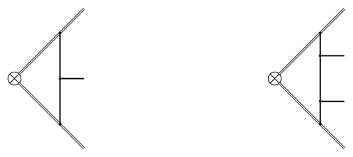
Figure 2: Topology classifications, with double-line referring to Wilson line

The set of master-integrals in our problem can be classified into two topologies as depicted in Figure 2. The first corresponds to single soft emission. The propagator list for the second pentagon topology is

$$\Bigg{\{}k^{2}+i\eta,\,(k+q_{2})^{2}+i\eta,\,(k-q_{3})^{2}+i\eta,\,-n_{1}\cdot(k+q_{2})-i\eta,\,n_{4}\cdot(k-q_{3})-i\eta\Bigg{\}}\,.$$ (88)

The results for soft triangle or soft box can be achieved by traditional Feynman parameter approach. To obtain the soft pentagon integral Bern:1993kr , traditional differential equations could be too involved to solve, the proposal here is to formulate differential equations with respect to a parameter Papadopoulos:2014lla .

To this end we define a new topology with a parameter $z$, which amounts to replacing $q_{2}$ with $zq_{2}$:

$$\Bigg{\{}k^{2},\,(k+zq_{2})^{2},\,(k-q_{3})^{2},\,-n_{1}\cdot(k+zq_{2}),\,n_{4}\cdot(k-q_{3})\Bigg{\}}\,.$$ (89)

Now each master integral carries the parameter $z$, and the soft triangle or soft box are obtained by replacing $q_{2}$ with $zq_{2}$ in their results Eq. (104). For the pentagon integral $I_{z;11111}$ we form an differential equation with respect to $z$, in doing so we define three rescaling invariants for the current problem:

$$x\equiv{s_{14}s_{23}\over(s_{12}+s_{13})(s_{24}+s_{34})}\,,\quad t\equiv\frac{s_{12}}{s_{12}+s_{13}}\,,\quad s\equiv\frac{s_{24}}{s_{24}+s_{34}}\,,$$ (90)

and set without loss of generality

$$n_{1}\cdot n_{4}=2\,,\quad q_{2}\cdot q_{3}=x/2\,,\quad n_{1}\cdot q_{2}=t\,,\quad n_{1}\cdot q_{3}=1-t\,,\quad n_{4}\cdot q_{2}=s\,,\quad n_{4}\cdot q_{3}=1-s\,.$$ (91)

Then the differential equation with respect to the parameter $z$ becomes

$$\partial_{z}\bigg{(}Q(z)I_{z;11111}\bigg{)}= \frac{Q(z)}{z\left(stz^{2}-2stz+st+sz-s+tz-t-xz+1\right)}$$ (92)

$$\,\times \bigg{\{}\frac{stz^{2}-st+s+t-1}{(s-1)tz(sz-s+1)(tz-t+1)}\,\epsilon\,I_{z;01100}$$ (93)

$$\,+ \frac{sz}{sz-s+1}(2\epsilon+1)I_{z;11011}-sz(2\epsilon+1)I_{z;11101}$$ (94)

$$\,+ \frac{(t-1)}{tz-t+1}(2\epsilon+1)I_{z;10111}-(t-1)(2\epsilon+1)I_{z;11110}\bigg{\}}\,,$$ (95)

where $Q(z)$ is a integration factor introduced such that the right hand side no longer depends on the pentagon itself

$$Q(z)\equiv z\left(stz^{2}-2stz+st+sz-s+tz-t-xz+1\right)^{\epsilon+1}\,.$$ (96)

The integration factor makes the problem a simple integration, but at the price of introducing a square root

$$Q(z)= z\left(st(z-r_{1})(z-r_{2})\right)^{\epsilon+1}\,,\quad\Delta(x,s,t)\equiv\sqrt{s^{2}+4stx-2st-2sx+t^{2}-2tx+x^{2}}\,.$$ (97)

$$\,r_{1}= \frac{-s-t+2st+x-\Delta(x,s,t)}{2st}\,,\quad\quad r_{2}=\frac{-s-t+2st+x+\Delta(x,s,t)}{2st}\,.$$ (98)

We are now left with the boundary conditions. In general the limit $z\rightarrow 0$ does not commute with the integration over the loop momentum and it seems that an independent calculation of the boundary term was necessary. But since the integration factor is proportional to $z$, it was conjectured and later confirmed that $Q(z)I_{z;11111}$ vanishes at the origin provided that $I_{z;11111}$ behaves regular at the origin (the same trick was also applied in Papadopoulos:2014lla ).

Below in Eq. (104) and Eq. (116) we collect the Euclidean results for the master integrals with a pre-factor of $c_{\Gamma}(-s_{23}-i\eta)^{-\epsilon}$

$$I^{\prime}_{01100} \equiv\frac{1-2\epsilon}{-2\epsilon}I_{01100}=-\frac{1}{2\epsilon^{2}}\,,\quad I_{10011}=\frac{\Gamma(1-2\epsilon)\Gamma(1+\epsilon)}{\epsilon^{2}\Gamma(1-\epsilon)}\frac{4}{s_{14}}\Bigg{(}\frac{s_{14}s_{23}}{s_{12}s_{34}}\Bigg{)}^{\epsilon}\,,$$ (99)

$$\,I_{11011} =\frac{\Gamma(1-2\epsilon)\Gamma(1+\epsilon)}{\epsilon^{2}\Gamma(1-\epsilon)}\frac{4}{s_{12}s_{34}}\left(\frac{s_{14}s_{23}}{s_{12}s_{34}}\right)^{\epsilon}\,_{2}F_{1}\left(1,1+\epsilon,1-\epsilon,-\frac{s_{24}}{s_{34}}\right)\,,$$ (100)

$$\,I_{11110} =-\frac{4}{s_{23}(s_{12}+s_{13})}\frac{1}{\epsilon^{2}}\,_{2}F_{1}\left(1,1,1-\epsilon,\frac{s_{13}}{s_{12}+s_{13}}\right)\,,$$ (101)

$$\,I_{01111} =\frac{\Gamma(1-2\epsilon)}{\Gamma^{2}(1-\epsilon)\Gamma(1+\epsilon)}\frac{4}{(s_{12}+s_{13})(s_{24}+s_{34})}\left(1-\frac{s_{14}s_{23}}{(s_{12}+s_{13})(s_{24}+s_{34})}\right)^{-1-\epsilon}$$ (102)

$$\times\bigg{\{}\frac{2\Gamma^{3}(1-\epsilon)\Gamma^{2}(1+\epsilon)}{\epsilon^{2}\Gamma(1-2\epsilon)}\left(\frac{s_{14}s_{23}}{(s_{12}+s_{13})(s_{24}+s_{34})}\right)^{\epsilon}-\frac{2\Gamma^{2}(1-\epsilon)\Gamma(1+\epsilon)}{\epsilon^{2}\Gamma(1-2\epsilon)}$$ (103)

$$\times\,_{2}F_{1}\left(-\epsilon,-\epsilon,1-\epsilon,\frac{s_{14}s_{23}}{(s_{12}+s_{13})(s_{24}+s_{34})}\right)\bigg{\}}\,.$$ (104)

$$I_{11111}=\frac{4}{s_{12}s_{34}(s_{12}+s_{13})(s_{24}+s_{34})s_{23}}\frac{1}{\epsilon^{2}}$$ (105)

$$\times\Bigg{\{}s_{34}(s_{12}+s_{13})\Bigg{[}1+\epsilon\ln\frac{s_{34}(s_{12}+s_{13})}{s_{12}(s_{24}+s_{34})}+\frac{1}{2}\epsilon^{2}\ln^{2}\frac{s_{34}(s_{12}+s_{13})}{s_{12}(s_{24}+s_{34})}\Bigg{]}$$ (106)

$$+(s_{12}+s_{13})(s_{24}+s_{34})\Bigg{[}1-\epsilon\ln\frac{s_{12}s_{34}}{(s_{12}+s_{13})(s_{24}+s_{34})}+\frac{1}{2}\epsilon^{2}\ln^{2}\frac{s_{12}s_{34}}{(s_{12}+s_{13})(s_{24}+s_{34})}\Bigg{]}$$ (107)

$$+s_{12}(s_{24}+s_{34})\Bigg{[}1+\epsilon\ln\frac{s_{12}(s_{24}+s_{34})}{s_{34}(s_{12}+s_{13})}+\frac{1}{2}\epsilon^{2}\ln^{2}\frac{s_{12}(s_{24}+s_{34})}{s_{34}(s_{12}+s_{13})}\Bigg{]}$$ (108)

$$-\frac{s_{14}s_{23}s_{34}(s_{12}+s_{13})}{(s_{12}+s_{13})(s_{24}+s_{34})-s_{23}s_{14}}\Bigg{[}\epsilon\ln\frac{s_{23}s_{14}}{(s_{12}+s_{13})(s_{24}+s_{34})}+\frac{1}{2}\epsilon^{2}\Bigg{(}\ln^{2}\frac{s_{14}s_{23}}{(s_{24}+s_{34})s_{12}}$$ (109)

$$+\ln^{2}\frac{s_{23}s_{14}}{(s_{12}+s_{13})(s_{24}+s_{34})}-\ln^{2}\frac{s_{14}s_{23}}{(s_{12}+s_{13})s_{34}}+\ln^{2}\frac{s_{34}}{s_{24}+s_{34}}-\ln^{2}\frac{s_{12}}{s_{12}+s_{13}}\Bigg{)}\Bigg{]}$$ (110)

$$-\frac{s_{14}s_{23}s_{12}(s_{24}+s_{34})}{(s_{12}+s_{13})(s_{24}+s_{34})-s_{23}s_{14}}\Bigg{[}\epsilon\ln\frac{s_{23}s_{14}}{(s_{12}+s_{13})(s_{24}+s_{34})}+\frac{1}{2}\epsilon^{2}\Bigg{(}\ln^{2}\frac{s_{14}s_{23}}{(s_{12}+s_{13})s_{34}}$$ (111)

$$+\ln^{2}\frac{s_{23}s_{14}}{(s_{12}+s_{13})(s_{24}+s_{34})}-\ln^{2}\frac{s_{14}s_{23}}{(s_{24}+s_{34})s_{12}}+\ln^{2}\frac{s_{12}}{s_{12}+s_{13}}-\ln^{2}\frac{s_{34}}{s_{24}+s_{34}}\Bigg{)}\Bigg{]}$$ (112)

$$+2s_{34}(s_{12}+s_{13})\epsilon^{2}\Bigg{[}\frac{\pi^{2}}{6}+\text{Li}_{2}\left(1-\frac{s_{24}+s_{34}}{s_{34}}\right)\Bigg{]}+2s_{12}(s_{24}+s_{34})\epsilon^{2}\Bigg{[}\frac{\pi^{2}}{6}+\text{Li}_{2}\left(1-\frac{s_{12}+s_{13}}{s_{12}}\right)\Bigg{]}$$ (113)

$$+2(s_{12}+s_{13})(s_{24}+s_{34})\epsilon^{2}\Bigg{[}\text{Li}_{2}\left(1-\frac{s_{34}}{s_{24}+s_{34}}\right)+\text{Li}_{2}\left(1-\frac{s_{12}}{s_{12}+s_{13}}\right)\Bigg{]}$$ (114)

$$+(s_{12}+s_{13})(s_{24}+s_{34})\frac{(s_{12}+s_{13})(s_{24}+s_{34})-s_{23}s_{14}-s_{34}(s_{12}+s_{13})-s_{12}(s_{24}+s_{34})}{(s_{12}+s_{13})(s_{24}+s_{34})-s_{23}s_{14}}$$ (115)

$$\times\epsilon^{2}\text{Li}_{2}\left(1-\frac{s_{23}s_{14}}{(s_{12}+s_{13})(s_{24}+s_{34})}\right)-(s_{12}+s_{13})(s_{24}+s_{34})\epsilon^{2}\frac{\pi^{2}}{3}\Bigg{\}}+\cal O(\epsilon)\,.$$ (116)

So far we have been presenting the main results in this work from section 3 to section 4, the checks we have done includes :

• By comparing our results with those subtracted from the one loop FDH amplitudes $\gamma^{*}$ $\rightarrow$ $q\bar{q}gg$ and $\gamma^{*}$ $\rightarrow$ $q\bar{q}$ $\bar{Q}Q$ Bern:1997sc ; Bern:1996ka .

• On-shell gauge invariance (see details in appendix A)

  $$q_{2\mu_{2}}{\mbox{\boldmath$J$}}_{a_{2}a_{3}}^{\mu_{2}\mu_{3}(1)}(q_{2},q_{3}) \propto\sum_{i=1}^{m}{\mbox{\boldmath$T$}}_{i}^{a}\;\;,$$ (117)

  $$q_{3\mu_{3}}{\mbox{\boldmath$J$}}_{a_{2}a_{3}}^{\mu_{2}\mu_{3}(1)}(q_{2},q_{3}) \propto\sum_{i=1}^{m}{\mbox{\boldmath$T$}}_{i}^{a}\;\;.$$ (118)

• Numeric checks of the master integrals using toolbox pySecDec Borowka:2017idc .

5 Analytical continuation

Recall our results are captured in time-like kinematics with positive Mandelstam variables, the corresponding topology with explicit prescription is

$${\rm{e^{+}e^{-}}}:\Bigg{\{}k^{2}+i\eta,\,(k+q_{2})^{2}+i\eta,\,(k-q_{3})^{2}+i\eta,\,-n_{1}\cdot(k+q_{2})-i\eta,\,n_{4}\cdot(k-q_{3})-i\eta\Bigg{\}}\,.$$ (119)

The crossing into ingoing states amounts to reversing some of the hard momenta , say $n_{1}\rightarrow-n_{1}$ ( $n_{4}\rightarrow-n_{4}$ ), or equivalently one still insists on a physical hard momentum with positive energy, etc. $n_{1}^{0}>0$ and $n_{4}^{0}>0$, but change accordingly the prescriptions. We take the latter method so we still have positive Mandelstam variables, in this way we can obtain other relevant topologies with different prescriptions :

$${\rm{DIS}}:\Bigg{\{}k^{2}+i\eta,\,(k+q_{2})^{2}+i\eta,\,(k-q_{3})^{2}+i\eta,\,-n_{1}\cdot(k+q_{2})+i\eta,\,n_{4}\cdot(k-q_{3})-i\eta\Bigg{\}}\,,$$ (120)

$$\,{\rm{DY}}:\Bigg{\{}k^{2}+i\eta,\,(k+q_{2})^{2}+i\eta,\,(k-q_{3})^{2}+i\eta,\,-n_{1}\cdot(k+q_{2})+i\eta,\,n_{4}\cdot(k-q_{3})+i\eta\Bigg{\}}\,.$$ (121)

Below we will perform analytical continuations from topology ${\rm{e^{+}e^{-}}}$ to topology ${\rm{DIS}}$ and topology ${\rm{DY}}$ for the master integrals and the soft amplitudes.

5.1 Analytical continuation of the master integrals

Recall we have made three rescaling invariants for the topologies

$$x\equiv{s_{14}s_{23}\over(s_{12}+s_{13})(s_{24}+s_{34})}\,,\quad t\equiv\frac{s_{12}}{s_{12}+s_{13}}\,,\quad s\equiv\frac{s_{24}}{s_{24}+s_{34}}\,.$$ (122)

By reversing a single Wilson line, the phase factor cancels in the numerator and denominator of each invariant, so no continuation is actually needed. By reversing two Wilson lines at the same time, we will have

$$x\rightarrow|x|e^{-2\pi i}\,,\quad\quad t\rightarrow t\,,\quad\quad s\rightarrow s\,.$$ (123)

The strategy is then taking a expansion around phase space region $q_{2}\parallel q_{3}$ or equivalently $x\rightarrow 0$. For example,

$$\lim_{x\rightarrow 0}\text{Li}_{2}(1-x) =-\ln(x)\sum_{n}\frac{(-x)^{n}}{n}+\dots=-\ln(x)\ln(1-x)+\dots\,,$$ (124)

$$\lim_{x\rightarrow 0}\text{Li}_{3}(1-x) =-\ln(x)\times\frac{-1}{2}\ln^{2}(1-x)+\dots\,.$$ (125)

Such functions fail to have Laurent expansions around the origin $x\rightarrow 0$ due to collinear enhancement proportional to $\ln(x)$, which result in discontinuities

$${\rm{disc.}}\left[\ln(x)\right] =-2\pi i\,,$$ (126)

$${\rm{disc.}}\left[\text{Li}_{2}(1-x)\right] =2\pi i\,\ln(1-x)\,,$$ (127)

$${\rm{disc.}}\left[\text{Li}_{3}(1-x)\right] =\pi i\,\ln^{2}(1-x)\,.$$ (128)

In section 4 we have obtained the Euclidean results for the master integrals. The analytical continuation to physical region where both Wilson lines are outgoing (for configurations like $\gamma^{*}\rightarrow$ 4 partons) is trivially obtained by

$$(-s_{23}-i\eta)^{-\epsilon}\rightarrow\lvert s_{23}\rvert e^{i\pi\epsilon}\,.$$ (129)

If some of the Wilson lines correspond to initial state, the rules is then clarified in Eq. (126) and we conclude

• No distinction between both outgoing and one of the Wilson lines outgoing.

• If both Wilson lines are ingoing, only box $I_{01111}$ and pentagon $I_{11111}$ develops nontrivial analytical continuation behaviors.

For the soft box $I_{01111}$ we have the following result for both ingoing Wilson line

$$I^{\rm{ingoing}}_{01111} =\frac{\Gamma(1-2\epsilon)}{\Gamma^{2}(1-\epsilon)\Gamma(1+\epsilon)}\frac{4}{(s_{12}+s_{13})(s_{24}+s_{34})}\left(1-\frac{s_{14}s_{23}}{(s_{12}+s_{13})(s_{24}+s_{34})}\right)^{-1-\epsilon}$$ (130)

$$\times\bigg{\{}\frac{2\Gamma^{3}(1-\epsilon)\Gamma^{2}(1+\epsilon)}{\epsilon^{2}\Gamma(1-2\epsilon)}\left(\frac{s_{14}s_{23}}{(s_{12}+s_{13})(s_{24}+s_{34})}\right)^{\epsilon}e^{-2\pi i\epsilon}-\frac{2\Gamma^{2}(1-\epsilon)\Gamma(1+\epsilon)}{\epsilon^{2}\Gamma(1-2\epsilon)}$$ (131)

$$\times\,_{2}F_{1}\left(-\epsilon,-\epsilon,1-\epsilon,\frac{s_{14}s_{23}}{(s_{12}+s_{13})(s_{24}+s_{34})}\right)\bigg{\}}\,.$$ (132)

For the pentagon, the corresponding result with both ingoing Wilson lines can be obtained by replacing in Eq (116)

$$\ln\frac{s_{23}s_{14}}{(s_{12}+s_{13})s_{34}}\rightarrow \ln\frac{s_{23}s_{14}}{(s_{12}+s_{13})s_{34}}-2\pi i\,,$$ (133)

$$\,\ln\frac{s_{23}s_{14}}{s_{12}(s_{24}+s_{34})}\rightarrow \ln\frac{s_{23}s_{14}}{s_{12}(s_{24}+s_{34})}-2\pi i\,,$$ (134)

$$\,\ln\frac{s_{23}s_{14}}{(s_{12}+s_{13})(s_{24}+s_{34})}\rightarrow \ln\frac{s_{23}s_{14}}{(s_{12}+s_{13})(s_{24}+s_{34})}-2\pi i\,,$$ (135)

$$\,\text{Li}_{2}\left(1-\frac{s_{23}s_{14}}{(s_{12}+s_{13})(s_{24}+s_{34})}\right)\rightarrow \text{Li}_{2}\left(1-\frac{s_{23}s_{14}}{(s_{12}+s_{13})(s_{24}+s_{34})}\right)$$ (136)

$$\,+ 2\pi i\ln\left(1-\frac{s_{23}s_{14}}{(s_{12}+s_{13})(s_{24}+s_{34})}\right)\,.$$ (137)

5.2 Drell Yan TMD Soft Function Vs. DIS TMD Soft Function Vs. $e^{+}e^{-}$ TMD Soft Function

Another application of our analytical continuation rules is to give a direct technical proof of the statement in Moult:2018jzp , that the Drell Yan and DIS and $e^{+}e^{-}$ Soft Function all equals up to three-loop, similar considerations and statements can also be found in Kang:2015moa ; Rothstein:2016bsq . Indeed we found that

$$\mathcal{M}_{a_{2}a_{3}}^{\rm{DIS}}- \mathcal{M}_{a_{2}a_{3}}^{\rm{e^{+}e^{-}}}=0\,.$$ (139)

$$\mathcal{M}_{a_{2}a_{3}}^{\rm{DY}}(2^{+},3^{+})- \mathcal{M}_{a_{2}a_{3}}^{\rm{DIS}}(2^{+},3^{+})=4{\left(\frac{s_{23}}{\mu^{2}}\right)^{-\epsilon}}\sum_{i\neq j}^{2}f_{bca_{2}}f_{bda_{3}}{\mbox{\boldmath$T$}}^{c}_{i}{\mbox{\boldmath$T$}}^{d}_{j}{\left\langle i\,j\right\rangle\over\left\langle i\,2\right\rangle\left\langle 2\,3\right\rangle\left\langle 3\,j\right\rangle}$$ (140)

$$\,\times (-2\pi i)\bigg{[}\frac{1}{\epsilon}+\ln\frac{{s_{ij}s_{23}\over(s_{i2}+s_{i3})(s_{2j}+s_{3j})}}{1-{s_{ij}s_{23}\over(s_{i2}+s_{i3})(s_{2j}+s_{3j})}}\bigg{]}+\cal O(\epsilon)\,,$$ (141)

$$\mathcal{M}_{a_{2}a_{3}}^{\rm{DY}}(2^{+},3^{-})- \mathcal{M}_{a_{2}a_{3}}^{\rm{DIS}}(2^{+},3^{-})=-4{\left(\frac{s_{23}}{\mu^{2}}\right)^{-\epsilon}}\sum_{i\neq j}^{2}f_{bca_{2}}f_{bda_{3}}{\mbox{\boldmath$T$}}^{c}_{i}{\mbox{\boldmath$T$}}^{d}_{j}\times(-2\pi i)$$ (142)

$$\,\times \bigg{[}{{1\over\left\langle i\,2\right\rangle\left[2\,j\right]+\left\langle i\,3\right\rangle\left[3\,j\right]\,}\left({1\over s_{i2}+s_{i3}}{\left[i\,j\right]\left\langle i\,3\right\rangle^{3}\over\left\langle 2\,3\right\rangle\left\langle i\,2\right\rangle}+{1\over s_{2j}+s_{3j}}{\left\langle i\,j\right\rangle\left[2\,j\right]^{3}\over\left[2\,3\right]\left[3\,j\right]}\right)}$$ (143)

$$\,\times \left(-\frac{1}{\epsilon}+\ln{s_{ij}s_{23}\over s_{i2}s_{3j}}\right)$$ (144)

$$\,+ {\left\langle i\,j\right\rangle\over\left\langle i\,2\right\rangle\left\langle 2\,j\right\rangle}{\left[i\,j\right]\over\left[i\,3\right]\left[3\,j\right]}\times\bigg{(}\ln{s_{ij}s_{23}\over s_{i2}s_{3j}}\bigg{)}$$ (145)

$$\,+ {1\over s_{i2}+s_{i3}}\Bigg{(}{-1\over\left\langle i\,2\right\rangle\left[2\,j\right]+\left\langle i\,3\right\rangle\left[3\,j\right]\,}{\left[i\,j\right]\left\langle i\,3\right\rangle^{3}\over\left\langle 2\,3\right\rangle\left\langle i\,2\right\rangle}+{-1\over\left[i\,2\right]\left\langle 2\,j\right\rangle+\left[i\,3\right]\left\langle 3\,j\right\rangle\,}{\left\langle i\,j\right\rangle\left[i\,2\right]^{3}\over\left[2\,3\right]\left[i\,3\right]}\Bigg{)}$$ (146)

$$\,\times \ln{s_{ij}s_{23}\over(s_{i2}+s_{i3})s_{3j}}$$ (147)

$$\,+ {1\over s_{2j}+s_{3j}}\Bigg{(}{-1\over\left\langle i\,2\right\rangle\left[2\,j\right]+\left\langle i\,3\right\rangle\left[3\,j\right]\,}{\left\langle i\,j\right\rangle\left[2\,j\right]^{3}\over\left[2\,3\right]\left[3\,j\right]}+{-1\over\left[i\,2\right]\left\langle 2\,j\right\rangle+\left[i\,3\right]\left\langle 3\,j\right\rangle\,}{\left[i\,j\right]\left\langle 3\,j\right\rangle^{3}\over\left\langle 2\,3\right\rangle\left\langle 2\,j\right\rangle}\Bigg{)}$$ (148)

$$\,\times \ln{s_{ij}s_{23}\over(s_{2j}+s_{3j})s_{i2}}\bigg{]}+\cal O(\epsilon)\,.$$ (149)

The differences are proportional to $2\pi i$ , and cancels when combined with their complex conjugation, thus the Virtual-Real-Real correction is universal. Since we know the triple-real contribution does not develop crossing issues, and the existing results for the double virtual real Duhr:2013msa ; Li:2013lsa and virtual real square Catani:2000pi contribution clearly shows a universality because of their global phase factor, we can conclude that the three-loop soft function is universal.

6 Conclusions

In this work we presented compact amplitude expressions of double soft gluons and double soft quarks emissions with generic color structure. Since gauge redundancy is inherent in color space formalism, we however found that the amplitude is best described in helicity variables to minimize the redundancy Dixon:1996wi . In general we found that the one-loop soft amplitude can be cast into an abelian contribution (for gluon) plus an non-abelian color correlated emission, the latter couples to two hard legs at one time.

We took strong ordering of the soft amplitude and obtained a factorized expression of two successive eikonal emission. We also talked about analytical continuation properties of the soft amplitude, and found non-vanishing discontinuities in going into initial states. However, the discontinuities turns out to be purely imaginary, which shows that the squared amplitude is invariant under crossing. Phenomenologically, this demonstrates the equivalence of DY, DIS and $e^{+}e^{-}$ TMD soft function up to three-loop, which was taken by default in the work Li:2020bub .

Combined with the known results for two-loop single soft amplitude that couples up to three hard particles Dixon:2019lnw , and the tree-level triple soft emissions which square to give a quadruple correlation Catani:2019nqv , the picture of NNNLO soft correlations with multiple hard legs becomes clear, which promotes a further step into the calculation of TMD soft function with multiple soft Wilson lines and the investigation of factorization violation Gao:2019ojf .

Appendix A Gauge invariance and color conservation

In this section, we introduce color space formalism Catani:2000pi and talk about relations between gauge invariance and color conservation.

Consider a generic scattering process that involves $m$ external massless QCD partons and arbitrary number and type of colorless particles in the physical region. The color space for that $m$ partons are tensor product of each single particle color space, and the basis vector is

$$|c_{1},...,c_{m}\rangle\equiv|c_{1}\rangle\otimes...\otimes|c_{m}\rangle\,,$$ (150)

with $c_{i}$ denoting the color content of $i_{\text{th}}$ parton. And consider the amplitude for the process being a vector in the color space of those $m$ partons

$$|\mathcal{M}_{m}^{s_{1},...,s_{m};\dots}(p_{1},...,p_{m})\rangle=\mathcal{M}_{m}^{c_{1},...,c_{m};s_{1},...,s_{m};\dots}(p_{1},...,p_{m})|c_{1},...,c_{m}\rangle\,,$$ (151)

where $s_{i}$ denotes helicity information or more degrees of freedom. The color charge operator of $i_{\text{th}}$ parton is now extended to the whole space, defined naturally as tensor products of identity operator acting on the color space of other partons

$$T^{a}_{i}\rightarrow{\mbox{\boldmath$T$}}^{a}_{i}\equiv\otimes^{i-1}_{1}\mathds{1}\otimes T^{a}_{i}\otimes\otimes^{m}_{i+1}\mathds{1}\,,\quad\quad\otimes^{j}_{i}\mathds{1}\equiv\mathds{1}_{i}\otimes\mathds{1}_{i+1}\otimes\dots\otimes\mathds{1}_{j}\,.$$ (152)

The matrix element reads

$$\langle c_{1},...,c_{m}|{\mbox{\boldmath$T$}}_{i}^{a}|b_{1},...,b_{m}\rangle\equiv\delta_{c_{1}b_{1}}...T_{c_{i},b_{i}}^{a}...\delta_{c_{m}b_{m}},$$ (153)

where $T_{cb}^{a}=if_{cab}$ if the emitting parton i is a gluon and $T_{\alpha\beta}=t_{\alpha\beta}^{a}$ if the emitting parton is a final state quark or an initial-state antiquark, and $T_{\alpha\beta}^{a}=\bar{t}_{\alpha\beta}^{a}=-t_{\beta\alpha}^{a}$ if it is a final-state antiquark or an initial-state quark.

Now writing the amplitude in terms of LSZ reduction procedure

$$\mathcal{M}^{a,\,i,\,j,\,\dots;s_{q},s_{\bar{q}},\dots} (P_{g},P_{q},P_{\bar{q}},\dots)=$$

$$\bigg{\{}\int dX_{g}e^{-iP_{g}X_{g}}\varepsilon^{\mu}\square_{\mu\nu}\int dX_{q}e^{-iP_{q}X_{q}}\bar{u}_{s_{q}}(P_{q})\overrightarrow{\ooalign{$\hfil/\hfil$\crcr$\partial$}_{q}}\dots$$ (156)

$$\langle\Omega|T\bigg{\{}A_{a}^{\nu}(X_{g})\Psi_{i}(X_{q})\bar{\Psi}_{j}(X_{\bar{q}})\dots\bigg{\}}|\Omega\rangle\dots\int dX_{\bar{q}}e^{iP_{\bar{q}}X_{\bar{q}}}u_{s_{\bar{q}}}(P_{\bar{q}})\overleftarrow{\ooalign{$\hfil/\hfil$\crcr$\partial$}_{\bar{q}}}\bigg{\}}_{c.}\,,$$ (159)

and performing a global gauge transformation ($\phi=A^{\nu},\Psi,\bar{\Psi}$; $R=\text{A},\text{F},\text{F}^{*}$)

$$\phi_{i}\rightarrow(1-i\theta^{a}T^{a}_{R})_{i\,j}\phi_{j}\,,$$ (160)

we demand the amplitude to be invariant under such a global transformation, i.e. $|\mathcal{M}\rangle$ is a color singlet

$$e^{-i\theta\cdot{\mbox{\boldmath$T$}}}|\mathcal{M}\rangle=|\mathcal{M}\rangle\Longleftrightarrow{{\mbox{\boldmath$T$}}}^{a}|\mathcal{M}\rangle=0\,,\quad\quad{\mbox{\boldmath$T$}}^{a}\equiv\sum_{i}{{\mbox{\boldmath$T$}}^{a}_{i}}\,.$$ (161)

We thus conclude color conservation is equivalent to global gauge invariance, which is typical of Noether theorem in quantum field theory.

We move on to show on-shell gauge invariance of the soft current. Suppose we perform a gauge transformation, under which the soft current gains an extra term of divergence:

$$\varepsilon_{\mu}(q)\rightarrow\varepsilon_{\mu}(q)+q_{\mu}\,,\quad\quad\varepsilon(q)\cdot{{\mbox{\boldmath$J$}}} (q)\rightarrow\varepsilon(q)\cdot{{\mbox{\boldmath$J$}}}(q)+q\cdot{{\mbox{\boldmath$J$}}}(q)\,.$$ (162)

But the extra term $q\cdot{{\mbox{\boldmath$J$}}}(q)$ must vanish when acting on a hard amplitude, thus by Eq. (161) the divergence must be proportional to the total charge of the hard amplitude

$$q\cdot{{\mbox{\boldmath$J$}}}(q)= \sum_{i}{{\mbox{\boldmath$T$}}^{a}_{i}}\,,\quad\quad\forall a\in\{1,2,\dots,8\}\,.$$ (163)

Appendix B Regularization scheme dependence

The soft amplitude in Eq.( 36), Eq.( 44) and Eq.( 76) develop dimensional regularization scheme dependence, the difference between $\rm FDH\,(\delta_{R}=0)$ and $\rm HV\,(\delta_{R}=1)$ reads

$${\mbox{\boldmath$J$}}_{a_{2}a_{3}}^{\mu_{2}\mu_{3}(1)}(q_{2},q_{3})|_{\delta_{R}=0}-{\mbox{\boldmath$J$}}_{a_{2}a_{3}}^{\mu_{2}\mu_{3}(1)}(q_{2},q_{3})|_{\delta_{R}=1}=0+\mathcal{O}(\epsilon)\,,$$ (164)

$$({{\mbox{\boldmath$J$}}}^{(1)})_{i_{2}}^{~{}{\;\bar{\imath}}_{3}}(q_{2},q_{3}) |_{\delta_{R}=0}-({{\mbox{\boldmath$J$}}}^{(1)})_{i_{2}}^{~{}{\;\bar{\imath}}_{3}}(q_{2},q_{3})|_{\delta_{R}=1}={\left(\frac{-s_{23}-i\eta}{\mu^{2}}\right)^{-\epsilon}}$$ (165)

$$\times \left(\frac{1}{2N_{c}(\epsilon-1)}-\frac{N_{c}}{2(\epsilon-1)(2\epsilon-3)(2\epsilon-1)}\right)({{\mbox{\boldmath$J$}}}^{(0)})_{i_{2}}^{~{}{\;\bar{\imath}}_{3}}(q_{2},q_{3})\,,$$ (166)

$$\,= \Bigg{(}\frac{1}{6}N_{c}-\frac{1}{2N_{c}}\Bigg{)}({{\mbox{\boldmath$J$}}}^{(0)})_{i_{2}}^{~{}{\;\bar{\imath}}_{3}}(q_{2},q_{3})+\mathcal{O}(\epsilon)\,.$$ (167)

The difference can be reproduced by considering the soft limit of full theory one-loop QCD amplitude.

	Conventional	’t Hooft–	Four
	dimensional	Veltman	dimensional
	regularization		helicity
	CDR	HV	FDH
Number of internal dimensions	$d$	$d$	$d$
Number of external dimensions	$d$	4	$4$
Number of internal gluons, $h_{g}$	$d-2$	$d-2$	2
Number of external gluons, $n_{s}(g)$	$d-2$	2	2
Number of internal quarks, $h_{q}$	2	2	2
Number of external quarks, $n_{s}(q)$	2	2	2

Table 1: Definitions of various regularization prescriptions of one-loop amplitudes in Ref Catani:1996pk .

To this end, we utilize the universal properties of infrared and ultraviolet poles of QCD amplitude Catani:2000ef ; Catani:1998bh ; Catani:1996pk , whose explicit expression depends on numbers of dimensions and polarizations (internal or external, see in Table 1), thus develops a RS dependence Gnendiger:2017pys ; Gnendiger:2019vnp .

First consider the perturbative expansion of a mass-renormalized amplitude in terms of bare strong coupling $g_{s}$

$$\mathcal{A}_{m}(g_{s},\mu^{2};\{p_{i},m_{i}\})=\left(\frac{g_{s}\mu^{\epsilon}}{4\pi}\right)^{q}\,\left[\,\mathcal{A}_{m}^{(0)}(\{p_{i},m_{i}\})+\left(\frac{g_{s}}{4\pi}\right)^{2}\,\mathcal{A}_{m}^{(1)}(\mu^{2};\{p_{i},m_{i}\})+{\mathcal{O}}(g_{s}^{4})\right]\,,$$ (168)

where $q$ fix the normalization, and $\mu$ is the dimensional-regularization scale.

In the massless case the sub-amplitude $\mathcal{A}_{m}^{(1)}$ allows a process-independent factorization formula Catani:1996pk ; Catani:2000ef ; Catani:1998bh

$$|\mathcal{A}_{m}^{(1)}(\mu^{2};\{p_{i},m_{i}\})\rangle_{{\scriptscriptstyle\rm R\!.S\!.}}={{\mbox{\boldmath$I$}}}_{m}^{{\scriptscriptstyle\rm R\!.S\!.}}(\epsilon,\mu^{2};\{p_{i},m_{i}\})\,|\mathcal{A}_{m}^{(0)}(\{p_{i},m_{i}\})\rangle_{{\scriptscriptstyle\rm R\!.S\!.}}+|\mathcal{A}_{m}^{(1)\,{\rm fin}}(\mu^{2};\{p_{i},m_{i}\})\rangle+\mathcal{O}({\epsilon})\>.$$ (169)

All the $\epsilon$-poles and RS dependence are included in the factor $I$, so that the $\mathcal{A}_{m}^{(1)\,{\rm fin}}$ piece is finite and RS-independent. But to remind, the product of the RS-dependent terms of O$(\epsilon)$ in $\mathcal{A}_{m}^{(0)}$ and double poles $1/\epsilon^{2}$ in $I$ produces, in general, an RS dependence of $\mathcal{A}_{m}^{(1)}$ that begins at O$(1/\epsilon)$.

The explicit expression for ${{\mbox{\boldmath$I$}}}_{m}$ in terms of the color charges of the $m$ partons is Catani:2000ef :

$${{\mbox{\boldmath$I$}}}_{m}^{\scriptscriptstyle\rm R\!.S\!.}(\epsilon,\mu^{2};\{p_{i},m_{i}\})= \frac{(4\pi)^{\epsilon}}{\Gamma(1-\epsilon)}\Bigg{\{}q\,\frac{1}{2}\left(\frac{\beta_{0}}{\epsilon}-{\tilde{\beta}}_{0}^{{\scriptscriptstyle\rm R\!.S\!.}}\right)$$ (170)

$$\,+ \sum_{j,k=1\atop k\neq j}^{m}{{\mbox{\boldmath$T$}}}_{j}\cdot{{\mbox{\boldmath$T$}}}_{k}\left(\frac{\mu^{2}}{|s_{jk}|}\right)^{\epsilon}\left[{\cal V}^{(\rm cc)}_{jk}(s_{jk};m_{j},m_{k};\epsilon)+\frac{1}{v_{jk}}\,\left(\frac{1}{\epsilon}\,i\pi\,-\frac{\pi^{2}}{2}\right)\Theta(s_{jk})\right]$$ (171)

$$\,- \sum_{j=1}^{m}\Gamma_{j}^{{\scriptscriptstyle\rm R\!.S\!.}}(\mu,m_{j};\epsilon)\Bigg{\}}\>.$$ (172)

The RS dependence comes from two side, the first of which is of ultraviolet origin and is proportional to $q$, which can be removed by a redefinition of the bare strong coupling $g_{s}$. At one loop, it is parametrized by constant coefficient ${\tilde{\beta}}_{0}^{{\scriptscriptstyle\rm R\!.S\!.}}$, where

$${\tilde{\beta}}_{0}^{\rm{HV}}=0\;,\quad\quad\quad{\tilde{\beta}}_{0}^{\rm{FDH}}=\frac{1}{3}\,C_{A}\,.$$ (173)

The second has an infrared origin due to either soft or collinear singularities, and is parametrized by constant coefficient $\Gamma_{j}^{{\scriptscriptstyle\rm R\!.S\!.}}$

$$\Gamma_{g}^{{\scriptscriptstyle\rm R\!.S\!.}}(\mu,m_{\{F\}};\epsilon)= \frac{1}{\epsilon}\;\gamma_{g}-\tilde{\gamma}_{g}^{{\scriptscriptstyle\rm R\!.S\!.}}-\frac{2}{3}\,T_{R}\sum_{F=1}^{N_{F}}\;\ln\frac{m_{F}^{2}}{\mu^{2}}\;,$$ (174)

$$\,\Gamma_{q}^{{\scriptscriptstyle\rm R\!.S\!.}}(\mu,0;\epsilon)= \frac{1}{\epsilon}\;\gamma_{q}-\tilde{\gamma}_{q}^{{\scriptscriptstyle\rm R\!.S\!.}}\,.$$ (175)

The flavour coefficients $\gamma_{j}$ are

$$\gamma_{j=q,\bar{q}}=\frac{3}{2}\,C_{F}\>,\qquad\qquad\quad\;\;\gamma_{g}=\frac{11}{6}\,C_{A}-\frac{2}{3}\,T_{R}\,N_{f}\>.$$ (176)

The coefficients $\tilde{\gamma}_{j}^{{\scriptscriptstyle\rm R\!.S\!.}}$ parametrize the finite (for $\epsilon\rightarrow 0$) contributions related to the RS. The transition coefficients $\tilde{\gamma}_{j}^{{\scriptscriptstyle\rm R\!.S\!.}}$ that relate different RS are given by

$$\tilde{\gamma}^{\rm HV}_{j}=0\>,\qquad\tilde{\gamma}^{\rm FDH}_{j=q,{\bar{q}}}=\frac{1}{2}\,C_{F}\>,\qquad\tilde{\gamma}^{\rm FDH}_{j=g}=\frac{1}{6}\,C_{A}.$$ (177)

With the above weapons we can determine the difference between $\rm{HV}$ and $\rm{FDH}$ for the soft amplitude. According to the factorization theorems, we have

$$\mathcal{M}^{\rm{FDH}}-\mathcal{M}^{\rm{HV}}\,\,{{\buildrel q_{2},q_{3}\rightarrow 0\over{\longrightarrow}}}{{\mbox{\boldmath$J$}}}^{0}\left(|\mathcal{M}^{(1)}_{\rm{FDH}}\rangle-|\mathcal{M}^{(1)}_{\rm{HV}}\rangle\right)+\left({{\mbox{\boldmath$J$}}}^{(1)}_{\rm{FDH}}-{{\mbox{\boldmath$J$}}}^{(1)}_{\rm{HV}}\right)|\mathcal{M}^{(0)}\rangle\,.$$ (178)

where ${{\mbox{\boldmath$J$}}}^{0}$ is the tree-level soft current and ${{\mbox{\boldmath$J$}}}^{(1)}$ is the soft current at one-loop and $\mathcal{M}^{(1)}$ is the one-loop QCD virtual correction, taken $\gamma^{*}$ $\rightarrow$ ${\bar{q}}\,q$ as an example ,

$$\mathcal{M}^{(1)}_{\rm{FDH}}= \Bigg{(}\frac{1}{2}N_{c}-\frac{1}{2N_{c}}\Bigg{)}\frac{1}{\epsilon^{2}}(-2-3\epsilon-7\epsilon^{2})\mathcal{M}^{(0)}+\mathcal{O}(\epsilon)\,,$$ (179)

$$\mathcal{M}^{(1)}_{\rm{HV}}= \Bigg{(}\frac{1}{2}N_{c}-\frac{1}{2N_{c}}\Bigg{)}\frac{1}{\epsilon^{2}}(-2-3\epsilon-8\epsilon^{2})\mathcal{M}^{(0)}+\mathcal{O}(\epsilon)\,.$$ (180)

The difference for double gluon amplitude in QCD is

$$\mathcal{M}^{\rm{FDH}} -\mathcal{M}^{\rm{HV}}$$ (181)

$$=\Bigg{(}q\frac{1}{2}\left((-{\tilde{\beta}}_{0}^{\rm{FDH}})-(-{\tilde{\beta}}_{0}^{\rm{HV}})\right)+2\tilde{\gamma}^{\rm FDH}_{j=q,{\bar{q}}}-2\tilde{\gamma}^{\rm HV}_{j=q,{\bar{q}}}+2\tilde{\gamma}^{\rm FDH}_{j=g}-2\tilde{\gamma}^{\rm HV}_{j=g}\Bigg{)}\mathcal{M}^{tree}+\mathcal{O}(\epsilon)$$ (182)

$$\,\,{{\buildrel q_{2},q_{3}\rightarrow 0\over{\longrightarrow}}}\Bigg{(}2\frac{1}{2}(-\frac{1}{3}C_{A})+C_{F}+\frac{2}{6}C_{A}\Bigg{)}{{\mbox{\boldmath$J$}}}^{0}\mathcal{M}^{(0)}+\mathcal{O}(\epsilon)$$ (183)

$$=\Bigg{(}\frac{1}{2}N_{c}-\frac{1}{2N_{c}}\Bigg{)}{{\mbox{\boldmath$J$}}}^{0}\mathcal{M}^{(0)}+\mathcal{O}(\epsilon)\,.$$ (184)

One see cancellation between Eq. (180) and Eq. (184), which leads to the result in Eq. (164).

For the double soft quark amplitude, we have

$$\mathcal{M}^{\rm{FDH}}-\mathcal{M}^{\rm{HV}} =\Bigg{(}q\frac{1}{2}\left((-{\tilde{\beta}}_{0}^{\rm{FDH}})-(-{\tilde{\beta}}_{0}^{\rm{HV}})\right)+4\tilde{\gamma}^{\rm FDH}_{j=q,{\bar{q}}}-4\tilde{\gamma}^{\rm HV}_{j=q,{\bar{q}}}\Bigg{)}\mathcal{M}^{(0)}+\mathcal{O}(\epsilon)$$ (185)

$$\,\,{{\buildrel q_{2},q_{3}\rightarrow 0\over{\longrightarrow}}}\Bigg{(}2\frac{1}{2}(-\frac{1}{3}C_{A})+2C_{F}\Bigg{)}{{\mbox{\boldmath$J$}}}^{0}\mathcal{M}^{(0)}+\mathcal{O}(\epsilon)$$ (186)

$$=\Bigg{(}-\frac{1}{3}C_{A}+2C_{F}\Bigg{)}{{\mbox{\boldmath$J$}}}^{0}\mathcal{M}^{(0)}+\mathcal{O}(\epsilon)\,.$$ (187)

Then by taking into account the difference in virtual corrections, one gets the difference for double soft quark currents which is in agreement with Eq. (165)

$${{\mbox{\boldmath$J$}}}^{(1)}_{\rm{FDH}}-{{\mbox{\boldmath$J$}}}^{(1)}_{\rm{HV}}= \frac{1}{\mathcal{M}^{(0)}}\Bigg{(}(\mathcal{M}^{\rm{FDH}}-\mathcal{M}^{\rm{HV}})|_{q_{2}\rightarrow 0,q_{3}\rightarrow 0}-{{\mbox{\boldmath$J$}}}^{0}(\mathcal{M}^{(1)}_{\rm{FDH}}-\mathcal{M}^{(1)}_{\rm{HV}})\Bigg{)}$$ (188)

$$\,= \Bigg{(}-\frac{1}{3}C_{A}+C_{F}\Bigg{)}{{\mbox{\boldmath$J$}}}^{0}+\mathcal{O}(\epsilon)$$ (189)

$$\,= \Bigg{(}\frac{1}{6}N_{c}-\frac{1}{2N_{c}}\Bigg{)}{{\mbox{\boldmath$J$}}}^{0}+\mathcal{O}(\epsilon)\,.$$ (190)

References

• (1) J. C. Collins, D. E. Soper, and G. F. Sterman, Factorization of Hard Processes in QCD, Adv. Ser. Direct. High Energy Phys. $5$ (1989) 1–91, [hep-ph/0409313].
• (2) G. F. Sterman, Partons, factorization and resummation, TASI 95, in QCD and beyond. Proceedings, Theoretical Advanced Study Institute in Elementary Particle Physics, TASI-95, Boulder, USA, June 4-30, 1995, pp. 327–408, 1995. hep-ph/9606312.
• (3) G. F. Sterman, QCD and jets, in Physics in D >= 4. Proceedings, Theoretical Advanced Study Institute in elementary particle physics, TASI 2004, Boulder, USA, June 6-July 2, 2004, pp. 67–145, 2004. hep-ph/0412013.
• (4) A. Buckley et al., General-purpose event generators for LHC physics, Phys. Rept. $5$04 (2011) 145–233, [arXiv:1101.2599].
• (5) S. Catani and M. Seymour, A General algorithm for calculating jet cross-sections in NLO QCD, Nucl. Phys. B $4$85 (1997) 291–419, [hep-ph/9605323]. [Erratum: Nucl.Phys.B 510, 503–504 (1998)].
• (6) S. Frixione, Z. Kunszt, and A. Signer, Three jet cross-sections to next-to-leading order, Nucl. Phys. B $4$67 (1996) 399–442, [hep-ph/9512328].
• (7) A. Gehrmann-De Ridder, T. Gehrmann, and E. Glover, Antenna subtraction at NNLO, JHEP 𝟎09 (2005) 056, [hep-ph/0505111].
• (8) S. Catani and M. Grazzini, An NNLO subtraction formalism in hadron collisions and its application to Higgs boson production at the LHC, Phys. Rev. Lett. $9$8 (2007) 222002, [hep-ph/0703012].
• (9) M. Czakon, A novel subtraction scheme for double-real radiation at NNLO, Phys. Lett. B $6$93 (2010) 259–268, [arXiv:1005.0274].
• (10) R. Boughezal, K. Melnikov, and F. Petriello, A subtraction scheme for NNLO computations, Phys. Rev. D $8$5 (2012) 034025, [arXiv:1111.7041].
• (11) M. Czakon and D. Heymes, Four-dimensional formulation of the sector-improved residue subtraction scheme, Nucl. Phys. B $8$90 (2014) 152–227, [arXiv:1408.2500].
• (12) C. Anastasiou, C. Duhr, F. Dulat, F. Herzog, and B. Mistlberger, Real-virtual contributions to the inclusive Higgs cross-section at $N^{3}LO$, JHEP $1$2 (2013) 088, [arXiv:1311.1425].
• (13) W. B. Kilgore, One-loop single-real-emission contributions to $pp\rightarrow H+X$ at next-to-next-to-next-to-leading order, Phys. Rev. D $8$9 (2014), no. 7 073008, [arXiv:1312.1296].
• (14) C. Duhr and T. Gehrmann, The two-loop soft current in dimensional regularization, Phys. Lett. B $7$27 (2013) 452–455, [arXiv:1309.4393].
• (15) Y. Li and H. X. Zhu, Single soft gluon emission at two loops, JHEP $1$1 (2013) 080, [arXiv:1309.4391].
• (16) C. Duhr, T. Gehrmann, and M. Jaquier, Two-loop splitting amplitudes and the single-real contribution to inclusive Higgs production at N3LO, JHEP 𝟎02 (2015) 077, [arXiv:1411.3587].
• (17) F. Dulat and B. Mistlberger, Real-Virtual-Virtual contributions to the inclusive Higgs cross section at N3LO, arXiv:1411.3586.
• (18) Y. Li, A. von Manteuffel, R. M. Schabinger, and H. X. Zhu, N3LO Higgs boson and Drell-Yan production at threshold: The one-loop two-emission contribution, Phys. Rev. D $9$0 (2014), no. 5 053006, [arXiv:1404.5839].
• (19) C. Anastasiou, C. Duhr, F. Dulat, E. Furlan, F. Herzog, and B. Mistlberger, Soft expansion of double-real-virtual corrections to Higgs production at N3LO, JHEP 𝟎08 (2015) 051, [arXiv:1505.04110].
• (20) C. Anastasiou, C. Duhr, F. Dulat, and B. Mistlberger, Soft triple-real radiation for Higgs production at N3LO, JHEP 𝟎07 (2013) 003, [arXiv:1302.4379].
• (21) Y. Hamada and G. Shiu, Infinite Set of Soft Theorems in Gauge-Gravity Theories as Ward-Takahashi Identities, Phys. Rev. Lett. $1$20 (2018), no. 20 201601, [arXiv:1801.05528].
• (22) L. Rodina, Scattering Amplitudes from Soft Theorems and Infrared Behavior, Phys. Rev. Lett. $1$22 (2019), no. 7 071601, [arXiv:1807.09738].
• (23) K. Kampf, J. Novotny, M. Shifman, and J. Trnka, New Soft Theorems for Goldstone Boson Amplitudes, Phys. Rev. Lett. $1$24 (2020), no. 11 111601, [arXiv:1910.04766].
• (24) S. Badger, F. Buciuni, and T. Peraro, One-loop triple collinear splitting amplitudes in QCD, JHEP 𝟎09 (2015) 188, [arXiv:1507.05070].
• (25) V. Del Duca, C. Duhr, R. Haindl, A. Lazopoulos, and M. Michel, Tree-level splitting amplitudes for a quark into four collinear partons, JHEP 𝟎02 (2020) 189, [arXiv:1912.06425].
• (26) V. Del Duca, C. Duhr, R. Haindl, A. Lazopoulos, and M. Michel, Tree-level splitting amplitudes for a gluon into four collinear partons, arXiv:2007.05345.
• (27) S. Catani and M. Grazzini, Infrared factorization of tree level QCD amplitudes at the next-to-next-to-leading order and beyond, Nucl. Phys. $B$570 (2000) 287–325, [hep-ph/9908523].
• (28) L. J. Dixon, E. Herrmann, K. Yan, and H. X. Zhu, Soft gluon emission at two loops in full color, arXiv:1912.09370.
• (29) S. Catani, D. Colferai, and A. Torrini, Triple (and quadruple) soft-gluon radiation in QCD hard scattering, JHEP 𝟎01 (2020) 118, [arXiv:1908.01616].
• (30) Y. Li and H. X. Zhu, Bootstrapping Rapidity Anomalous Dimensions for Transverse-Momentum Resummation, Phys. Rev. Lett. $1$18 (2017), no. 2 022004, [arXiv:1604.01404].
• (31) I. Moult and H. X. Zhu, Simplicity from Recoil: The Three-Loop Soft Function and Factorization for the Energy-Energy Correlation, JHEP 𝟎08 (2018) 160, [arXiv:1801.02627].
• (32) A. Gao, H. T. Li, I. Moult, and H. X. Zhu, Precision QCD Event Shapes at Hadron Colliders: The Transverse Energy-Energy Correlator in the Back-to-Back Limit, Phys. Rev. Lett. $1$23 (2019), no. 6 062001, [arXiv:1901.04497].
• (33) S. Catani and M. Grazzini, The soft gluon current at one loop order, Nucl. Phys. $B$591 (2000) 435–454, [hep-ph/0007142].
• (34) Z. Bern, V. Del Duca, and C. R. Schmidt, The Infrared behavior of one loop gluon amplitudes at next-to-next-to-leading order, Phys. Lett. $B$445 (1998) 168–177, [hep-ph/9810409].
• (35) Z. Bern, V. Del Duca, W. B. Kilgore, and C. R. Schmidt, The infrared behavior of one loop QCD amplitudes at next-to-next-to leading order, Phys. Rev. $D$60 (1999) 116001, [hep-ph/9903516].
• (36) I. Feige and M. D. Schwartz, Hard-Soft-Collinear Factorization to All Orders, Phys. Rev. $D$90 (2014), no. 10 105020, [arXiv:1403.6472].
• (37) C. W. Bauer, D. Pirjol, and I. W. Stewart, Soft collinear factorization in effective field theory, Phys. Rev. D $6$5 (2002) 054022, [hep-ph/0109045].
• (38) Z. Bern and G. Chalmers, Factorization in one loop gauge theory, Nucl. Phys. $B$447 (1995) 465–518, [hep-ph/9503236].
• (39) Z. Bern, L. J. Dixon, and D. A. Kosower, One loop amplitudes for e+ e- to four partons, Nucl. Phys. $B$513 (1998) 3–86, [hep-ph/9708239].
• (40) Z. Bern, L. J. Dixon, D. A. Kosower, and S. Weinzierl, One loop amplitudes for e+ e- —> anti-q q anti-Q Q, Nucl. Phys. $B$489 (1997) 3–23, [hep-ph/9610370].
• (41) P. Nogueira, Automatic Feynman graph generation, J. Comput. Phys. $1$05 (1993) 279–289.
• (42) B. Ruijl, T. Ueda, and J. Ruijl:2017dtg, FORM version 4.2, arXiv:1707.06453.
• (43) Z. Bern and D. A. Kosower, The Computation of loop amplitudes in gauge theories, Nucl. Phys. $B$379 (1992) 451–561.
• (44) Z. Bern, A. De Freitas, L. J. Dixon, and H. L. Wong, Supersymmetric regularization, two loop QCD amplitudes and coupling shifts, Phys. Rev. $D$66 (2002) 085002, [hep-ph/0202271].
• (45) G. ’t Hooft and M. J. G. Veltman, Regularization and Renormalization of Gauge Fields, Nucl. Phys. $B$44 (1972) 189–213.
• (46) K. G. Chetyrkin and F. V. Tkachov, Integration by Parts: The Algorithm to Calculate beta Functions in 4 Loops, Nucl. Phys. $B$192 (1981) 159–204.
• (47) R. N. Lee, Presenting LiteRed: a tool for the Loop InTEgrals REDuction, arXiv:1212.2685.
• (48) S. Catani and L. Cieri, Multiple soft radiation at one-loop order and the emission of a soft quark-antiquark pair, arXiv:2108.13309.
• (49) Z. Bern, L. J. Dixon, and D. A. Kosower, Dimensionally regulated pentagon integrals, Nucl. Phys. $B$412 (1994) 751–816, [hep-ph/9306240].
• (50) C. G. Papadopoulos, Simplified differential equations approach for Master Integrals, JHEP 𝟎07 (2014) 088, [arXiv:1401.6057].
• (51) S. Borowka, G. Heinrich, S. Jahn, S. P. Jones, M. Kerner, J. Schlenk, and T. Zirke, pySecDec: a toolbox for the numerical evaluation of multi-scale integrals, Comput. Phys. Commun. $2$22 (2018) 313–326, [arXiv:1703.09692].
• (52) D. Kang, O. Z. Labun, and C. Lee, Equality of hemisphere soft functions for $e^{+}e^{-}$, DIS and $pp$ collisions at $\mathcal{O}(\alpha_{s}^{2})$, Phys. Lett. B $7$48 (2015) 45–54, [arXiv:1504.04006].
• (53) I. Z. Rothstein and I. W. Stewart, An Effective Field Theory for Forward Scattering and Factorization Violation, JHEP 𝟎08 (2016) 025, [arXiv:1601.04695].
• (54) L. J. Dixon, Calculating scattering amplitudes efficiently, in QCD and beyond. Proceedings, Theoretical Advanced Study Institute in Elementary Particle Physics, TASI-95, Boulder, USA, June 4-30, 1995, pp. 539–584, 1996. hep-ph/9601359.
• (55) H. T. Li, I. Vitev, and Y. J. Zhu, Transverse-Energy-Energy Correlations in Deep Inelastic Scattering, arXiv:2006.02437.
• (56) M. Czakon, F. Eschment, and T. Schellenberger, Revisiting the double-soft asymptotics of one-loop amplitudes in massless QCD, arXiv:2211.06465.
• (57) S. Catani, M. H. Seymour, and Z. Trocsanyi, Regularization scheme independence and unitarity in QCD cross-sections, Phys. Rev. $D$55 (1997) 6819–6829, [hep-ph/9610553].
• (58) S. Catani, S. Dittmaier, and Z. Trocsanyi, One loop singular behavior of QCD and SUSY QCD amplitudes with massive partons, Phys. Lett. $B$500 (2001) 149–160, [hep-ph/0011222].
• (59) S. Catani, The Singular behavior of QCD amplitudes at two loop order, Phys. Lett. $B$427 (1998) 161–171, [hep-ph/9802439].
• (60) C. Gnendiger et al., To ${d}$, or not to ${d}$: recent developments and comparisons of regularization schemes, Eur. Phys. J. $C$77 (2017), no. 7 471, [arXiv:1705.01827].
• (61) C. Gnendiger and A. Signer, Dimensional schemes for cross sections at NNLO, Eur. Phys. J. C $8$0 (2020), no. 3 215, [arXiv:1912.09974].