WASP-117 b: an eccentric hot-Saturn as a future complex chemistry laboratory

Abstract

We present spectral analysis of the transiting Saturn-mass planet WASP-117 b, observed with the G141 grism of the Hubble Space Telescope’s Wide Field Camera 3 (WFC3). We reduce and fit the extracted spectrum from the raw transmission data using the open-source software Iraclis before performing a fully Bayesian retrieval using the publicly available analysis suite TauREx 3.0. We detect water vapour alongside a layer of fully opaque cloud, retrieving a terminator temperature of $T_{term}=833^{+260}_{-156}$ K. In order to quantify the statistical significance of this detection, we employ the Atmospheric Detectability Index (ADI), deriving a value of ADI = 2.30, which provides positive but not strong evidence against the flat-line model. Due to the eccentric orbit of WASP-117 b, it is likely that chemical and mixing timescales oscillate throughout orbit due to the changing temperature, possibly allowing warmer chemistry to remain visible as the planet begins transit, despite the proximity of its point of ingress to apastron. We present simulated spectra of the planet as would be observed by the future space missions Ariel and JWST and show that, despite not being able to probe such chemistry with current HST data, these observatories should make it possible in the not too distant future.

1 Introduction

Among the gaseous exoplanets detected so far, a small subset are Saturn-mass ($\sim 0.3M_{J}$) with radii larger than $1R_{J}$, making their atmospheres inflated. Examples include WASP-69 b, Kepler-427 b, WASP-151 b and HAT-P-51 b (Anderson et al., 2014; Hébrard et al., 2014; Demangeon et al., 2018; Hartman et al., 2015). Most of these inflated hot-Saturns have been discovered using the transit method, which provides an observational bias towards lower eccentricity systems. Thus, eccentric hot-Saturns that have been discovered so far are fairly limited, including GJ 1148 b, which is not transiting and for which the radius is not constrained (Trifonov et al., 2018), and HAT-P-19 b, which is indeed inflated but has a relatively low eccentricity of $e\approx 0.067$ (Hartman et al., 2010). At the time of its discovery in 2014, WASP-117 b was the first planet found to possess a period larger than 10 days by the WASP survey, and at present remains the lowest mass gaseous planet with such a period, with a mass of $M_{p}=0.2755\pm 0.0089$ $M_{J}$ and a radius of $R_{p}=1.021^{+0.076}_{-0.065}$ $R_{J}$ (Lendl et al., 2014). With a well-constrained eccentricity of $e=0.302\pm 0.023$, WASP-117 b exhibits itself as an inflated Saturn-mass planet in an eccentric, misaligned orbit around a bright (V_mag = 10.15) main-sequence F9 star, a rarity among transiting gaseous extra-solar planets.

As a consequence of its large orbital distance, the tidal forces exerted on WASP-117 b by its host star are thought to be weak, making the planet’s eccentric orbit very stable over the system lifetime. Subsequently this planet provides an important case study for analysis of orbital dynamics and disc migration in gaseous exoplanets, as alluded to in Lendl et al. (2014). The eccentric nature of its orbit gives rise to fluctuations in the stellar flux received by the planet. This results in a variation in the temperature as WASP-117 b traverses its orbit, which in turn may cause changes in the corresponding chemistry. The thermal variations caused by the orbital parameters coupled with large chemical mixing timescales make this planet a tantalising and, at present, unique object for the study of exoplanet atmospheric chemistry. Fortunately, the lack of significant activity and brightness of its host star (Lendl et al., 2014) make WASP-117 b an excellent candidate for atmospheric characterisation.

In recent years the Hubble and Spitzer Space Telescopes have enabled the study of an increasing number of exoplanetary atmospheres through transit, eclipse, or phase-curve spectro-photometric observations (e.g. Vidal-Madjar et al., 2003; Swain et al., 2008; Laughlin et al., 2009; Linsky et al., 2010; Tinetti et al., 2010; Majeau et al., 2012; Deming et al., 2013; Fraine et al., 2014; Stevenson et al., 2014c; Morello et al., 2016; Evans et al., 2017; Skaf et al., 2020; Edwards et al., 2020a). Complementary observations from the ground, through high-dispersion or direct imaging spectroscopic techniques, have allowed for the extension of atmospheric observations to non-transiting planets (e.g. Macintosh et al., 2015; Brogi et al., 2012). While a handful of smaller planets have been observed (e.g. Kreidberg et al., 2014; Tsiaras et al., 2016c; de Wit et al., 2018; Demory et al., 2016; Kreidberg et al., 2019; Tsiaras et al., 2019; Benneke et al., 2019)), the current sample of observed exoplanetary atmospheres is still biased towards larger planets, which typically present a stronger signal to detect (e.g. Sing et al., 2016; Iyer et al., 2016; Tsiaras et al., 2018; Pinhas et al., 2019).

In this paper we present an analysis of the HST WFC3 G141 transmission spectrum of WASP-117 b. Our retrievals show evidence of water vapour but, due to the narrow spectral coverage (1.088 - 1.688 $\mu m$), we are unable to constrain the abundances of carbon-based molecules such as CH₄, CO and CO₂. The molecule which is perhaps most indicative of potential chemical changes over the orbit of WASP-117 b due to orbit-induced temperature variations is CH₄. Future space observatories and missions like JWST (Greene et al., 2016) and Ariel (Tinetti et al., 2018), with long spectral baselines, will enable us to widen and deepen our spectral view and subsequently reveal possible complex chemistry. We present simulations of equilibrium chemical profiles at WASP-117 b’s temperature extremes to demonstrate that, while the HST data is insufficient to distinguish between these cases, Ariel and JWST should have the precision and spectral coverage to disentangle these scenarios.

2 Methods

2.1 HST-WFC3 Data Analysis

Our analysis of the HST-WFC3 data started from the raw spatially scanned spectroscopic images which were obtained from the Mikulski Archive for Space Telescopes. The transmission spectrum of WASP-117 b was acquired by proposal 15301 and was taken in September 2019. We used Iraclis, a specialised, open-source software for the analysis of WFC3 scanning observations. The reduction process included the following steps: zero-read subtraction, reference pixels correction, non-linearity correction, dark current subtraction, gain conversion, sky background subtraction, calibration, flat-field correction, and corrections for bad pixels and cosmic rays. For a detailed description of these steps, we refer the reader to the original Iraclis papers (Tsiaras et al., 2016b, 2018, c).

The reduced spatially scanned spectroscopic images were then used to extract the white (1.088 - 1.688 $\mu$m) and spectral light curves. As is routinely done for HST studies, we then discarded the first orbit of the visit as it presents stronger wavelength pendant ramps. For the fitting of the white light curve, the only free parameters were the mid-transit time and planet-to-star ratio, with other values fixed to those from Lendl et al. (2014) ($P=10.020607$, $a/R_{s}=17.39$, $i=89.14$, $\omega=242$, $T_{0}=2457355.51373$). However, the white light curve fit showed significant residuals. We therefore fitted the light curve with the reduced semi-major axis, $a/R_{s}$, as an additional free parameter. We then performed a final white light curve fitting with our updated value of $a/R_{s}=17.65$. While some residuals remain, the divide-by-white method ensures these are not seen in the spectral light curves. The limb-darkening coefficients were selected from the best available stellar parameters using values from Claret et al. (2012, 2013) and using the stellar parameters from Lendl et al. (2014). The fitted white light curve for the transmission observation is shown in Figure 1 while the spectral light curves are plotted in Figure 2.

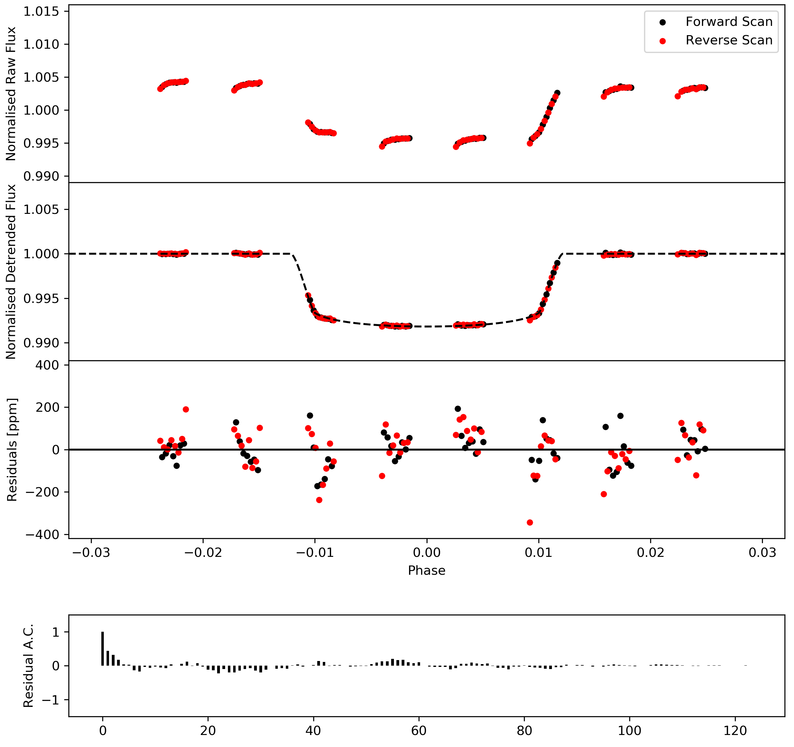
Figure 1: White light curve for the transmission observation of WASP-117 b. First panel: raw light curve, after normalisation. Second panel: light curve, divided by the best fit model for the systematics. Third panel: residuals for best-fit model. Fourth panel: auto-correlation function of the residuals.

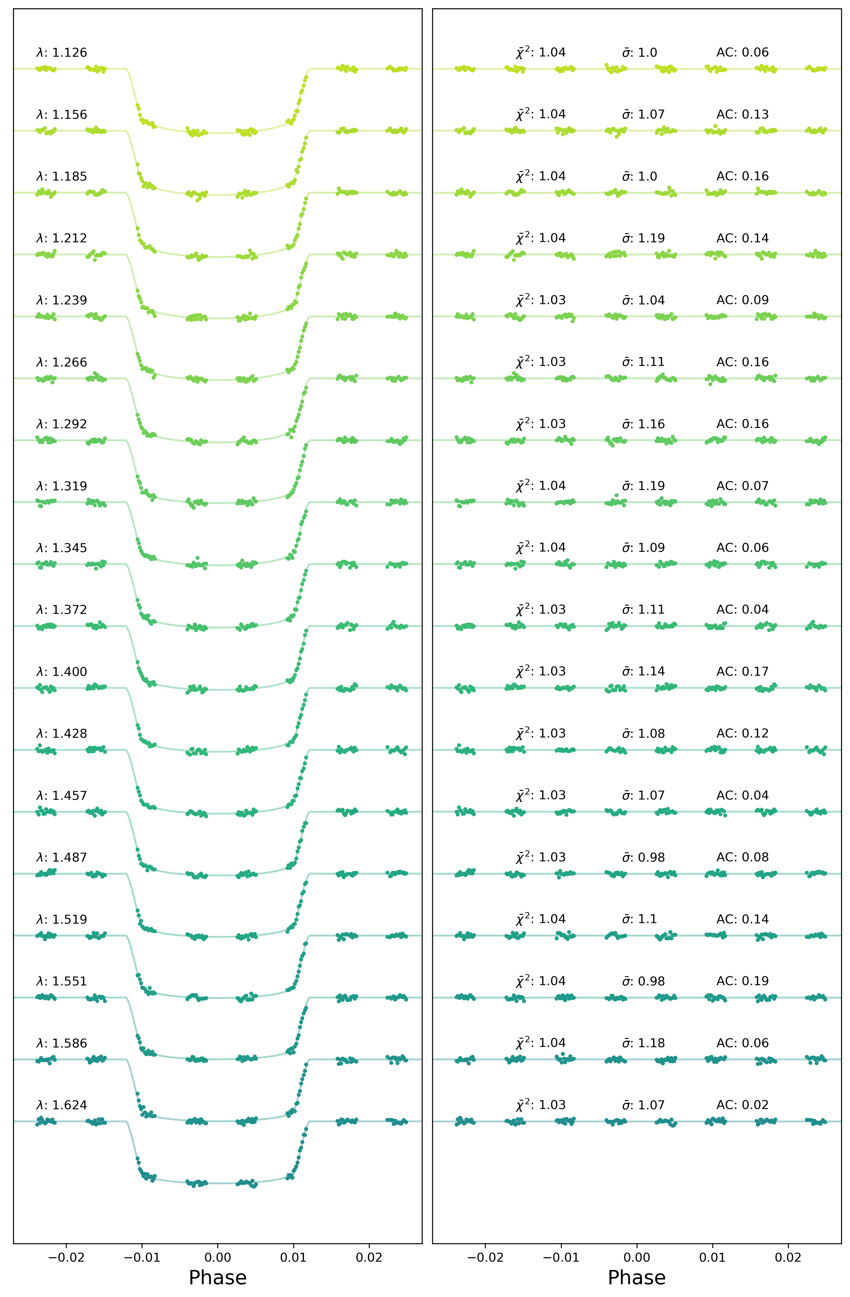
Figure 2: Spectral light curves fitted with Iraclis for the transmission spectra where, for clarity, an offset has been applied. Left: the detrended spectral light curves with best-fit model plotted. Right: residuals from the fitting with values for the Chi-squared ($\chi^{2}$), the standard deviation of the residuals with respect to the photon noise ($\bar{\sigma}$) and the auto-correlation (AC).

2.2 Ephemeris Refinement

Accurate knowledge of exoplanet transit times is fundamental for atmospheric studies. To ensure that WASP-117 b can be observed in the future, we used our HST white light curve mid time, along with data from TESS (Ricker et al., 2014), to update the ephemeris of the planet. TESS data is publicly available through the MAST archive and we use the pipeline from Edwards et al. (2020b) to download, clean and fit the 2 minute cadence Pre-search Data Conditioning (PDC) light curves (Smith et al., 2012; Stumpe et al., 2012, 2014). WASP-117 b had been studied in Sectors 2 and 3 and, after excluding bad data, we recovered 4 transits. These were fitted individually with the planet-to-star radius ratio ($R_{p}/R_{s}$), reduced semi-major axis ($a/R_{s}$), inclination ($i$) and transit mid time ($T_{mid}$) as free parameters.

2.3 Atmospheric Modelling

Due to the fact that WASP-117 b is in possession of an eccentric and misaligned orbit, it is thought that its atmosphere may exhibit significant changes in temperature as it traverses its orbit. We can estimate the temperature range by calculating the equilibrium (day-side) temperature expected at periastron and apastron, which we have calculated to be at a distance of approximately 0.067 AU and 0.124 AU from the host star, respectively. The day-side equilibrium temperature of a planet, $T_{p}$, at a distance $a$ from its host star can be derived as a result of equating the incident stellar flux on the planet with that which is absorbed by the planet:

$$T_{p}=T_{*}\sqrt{\frac{R_{*}}{2a}}\left(\frac{1-A}{\beta\epsilon}\right)^{\frac{1}{4}}$$ (1)

as given in Méndez & Rivera-Valentín (2017), where $\beta$ is a measure of the fraction of surface area over which the planet re-radiates the stellar flux that it absorbs, $\epsilon$ is the broadband thermal emissivity, and $A$ is the planetary surface albedo. The temperature and radius of the star are denoted as $T_{*}$ and $R_{*}$, respectively.

Considering the eccentricity of the orbit, it is likely that WASP-117 b is not tidally locked, possibly allowing for effective heat redistribution. Hence, using equation 1 with these assumptions, we take $\beta=1$ and $A=0.3$, obtaining equilibrium temperatures of $T_{p}=1116$ K and $T_{p}=817$ K at periastron and at apastron, respectively. Since the planet has an argument of periastron determined by Lendl et al. (2014) as $\omega=242.0^{+2.3}_{-2.7}$ degrees, we obtain a transit equilibrium temperature of $T_{p}=838$ K and expect to probe the terminator region of its atmosphere with the planet very close to its least irradiated region of its orbit.

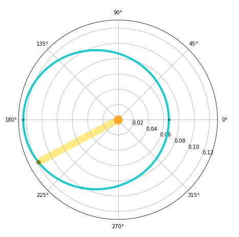
Figure 3: A schematic diagram of the orbital trajectory of WASP-117 b, where the shaded yellow region illustrates the line-of-sight direction that we observe during transit, confirming the proximity to apastron of this region.

We have estimated the possible chemical composition of the atmosphere by running equilibrium chemistry models for WASP-117 b at its temperature extremes. More specifically we used the ACE equilibrium chemistry package (Agúndez et al., 2012; Venot et al., 2012) contained in TauREx 3.0 to generate molecular abundances at the periastron and apastron equilibrium temperatures of 1100K and 800K, respectively. Together with input stellar parameters, given in Table 2, and retrieved values from WFC3 data for the planet’s radius and cloud pressure, these abundance profiles were then used as input for free-chemical forward models at the retrieved terminator temperature, in order to investigate what sort of chemistry might be visible during transit.

Transmission Spectrum
Wavelength	Transit Depth	Error	Bandwidth
$[\mu m]$	[%]	[%]	$[\mu m]$
1.12620	0.74725	0.00412	0.03080
1.15625	0.74810	0.00417	0.02930
1.18485	0.75177	0.00379	0.02790
1.21225	0.74688	0.00457	0.02690
1.23895	0.74374	0.00425	0.02650
1.26565	0.75076	0.00425	0.02690
1.29245	0.74048	0.00453	0.02670
1.31895	0.74098	0.00449	0.02630
1.34535	0.74622	0.00415	0.02650
1.37230	0.75244	0.00420	0.02740
1.4000	0.75249	0.00434	0.02800
1.42825	0.75465	0.00409	0.02850
1.45720	0.75548	0.00438	0.02940
1.48730	0.75104	0.00379	0.03080
1.51860	0.74379	0.00422	0.03180
1.55135	0.73922	0.00410	0.03370
1.58620	0.74068	0.00464	0.03600
1.62370	0.74473	0.00421	0.03900

Table 1: Reduced and fitted spectral data from the raw HST-WFC3 transmission data using Iraclis.

2.4 Spectral Retrieval Simulations

In order to extract the information content of WASP-117 b’s WFC3 transmission spectrum, retrieval analysis was performed using the publicly available retrieval suite TauREx 3.0 (Waldmann et al., 2015a, b; Al-Refaie et al., 2019), in addition to performing retrievals on our simulated Ariel and JWST spectra, discussed in Section 2.6. For the stellar parameters and the planet mass, we used the values from Lendl et al. (2014), as given in Table 2. In our runs we assumed that WASP-117 b possesses a primary atmosphere with fill gas abundance ratio of $V_{\text{He}}/V_{\text{H}_{2}}$ = 0.17, where $V_{x}$ denotes the volume mixing ratio for molecule $x.$ We included in our simulations the contribution of trace gases whose opacities were taken from the ExoMol (Tennyson et al., 2016)), HITRAN (Gordon et al., 2016) and HITEMP (Rothman & Gordon, 2014) databases for: H₂O (Polyansky et al., 2018), CH₄ (Yurchenko & Tennyson, 2014), CO (Li et al., 2015) and CO₂ (Rothman et al., 2010). Additionally, we included the Collision Induced Absorption (CIA) from H₂-H₂ (Abel et al., 2011; Fletcher et al., 2018) and H₂-He (Abel et al., 2012), as well as Rayleigh scattering for all molecules. In our retrieval analysis, we used uniform priors for all parameters as described in Table 3. Finally, we explored the parameter space using the nested sampling algorithm MultiNest (Feroz et al., 2009) with 1500 live points and an evidence tolerance of 0.5.

2.5 Atmospheric Detectability

We quantify the significance of our retrieval results by adopting the formalism of the Atmospheric Detectability Index (ADI) introduced in Tsiaras et al. (2018). The ADI is defined as the Bayes Factor, or likelihood ratio, between the retrieved atmospheric model (R) and the flat-line model (F), where the latter is designed to include known degeneracies between parameters in both models. Using the Bayes evidence of each model, as calculated as part of the retrieval, we may determine the ADI as follows:

$$\text{ADI}=\begin{cases}\ln\left(\frac{E_{R}}{E_{F}}\right)\quad\text{if}\quad\frac{E_{R}}{E_{F}}>1\\ 0\quad\quad\quad\quad\text{otherwise}\end{cases}$$ (2)

where $E_{R}$ and $E_{F}$ are the Bayes evidence for the retrieval model and the flat-line model, respectively. In our case, the retrieval model included the following contributions to opacity: molecular, simple fully-opaque clouds, collision-induced absorption due to H₂-H₂ and H₂-He, along with Rayleigh scattering. As for the flat-line model, we included only simple fully-opaque clouds. This ensures that the derived value of ADI gives a detection significance for the atmosphere detected whilst known degeneracies in each model between the radius of the planet, its temperature and the height of possible clouds, have been accounted for.

Stellar & Planetary Parameters
Parameter	Value
$T_{*}$ [K]	$6038$
$R_{*}$ [$R_{\odot}$]	1.170
$M_{*}$ [$M_{\odot}$]	1.126
$\log_{10}(g)_{*}$ [$cm/s^{2}$]	4.28
$[\text{Fe/H}]_{*}$	-0.11
$e$	$0.302$
$i$ [deg]	$89.14$
$\omega$ [deg]	$242.0$
$\Psi$ [deg]	69.6
$M_{p}$ [$M_{J}$]	0.276
$R_{p}$ [$R_{J}$]	1.021
$P_{orbital}$ [days]	10.02

Table 2: Stellar and planetary parameters for WASP-117 b, for input into Iraclis and TauREx 3.0, derived from Lendl et al. (2014).

2.6 Ariel & JWST simulations

Following on from Section 2.3, in order to investigate observable chemistry on WASP-117 b, we have simulated two different spectra assuming the planet and stellar parameters as specified in Table 2 and using TauREx 3.0 to generate chemical equilibrium forward models. Both forward models are created using the retrieved terminator temperature of 833 K, with one using chemical equilibrium molecular abundances expected for a 1100 K atmosphere and one using those for one at 800 K. We note that this does not account for disequilibrium processes such as quenched molecular abundances to deep atmospheric levels due to vertical mixing, for example. During its primary mission, Ariel will survey the atmospheres of 1000 exoplanets (Edwards et al., 2019) while JWST could observe up to 150 over the 5-year mission lifetime (Cowan et al., 2015). WASP-117 b is an excellent target for characterisation with either observatory and so we generate error bars for the simulated spectra using ArielRad (Mugnai et al., 2020) and ExoWebb (Edwards et al., 2020). For JWST we modelled observations with NIRISS GR700XD (0.8 - 2.8 $\mu m$) and NIRSpec G395M (2.9 - 5.3 $\mu m$), assuming 2 transit observations with each instrument whilst for Ariel, which provides simultaneous coverage from 0.5 - 7.8 $\mu m$, we simulated error bars at tier 3 resolution for 15 transit observations.

3 Results

3.1 HST-WFC3 Data Analysis and Interpretation

Our retrieval analysis determined the presence of water vapour with a volume mixing ratio, $V_{\text{H}_{2}\text{O}}$, given by $\log_{10}(V_{\text{H}_{2}\text{O}})=-3.82^{+1.37}_{-1.55}$, in the atmosphere of WASP-117 b. Additionally a layer of grey cloud at $10^{2.52^{+1.53}_{-1.25}}$ Pa was retrieved, with the parameter $P_{cloud}=\frac{P\text{[Pa]}}{1\text{[Pa]}}$ denoting the ratio between the atmospheric pressure at which the cloud layer sits, and 1 Pa, to provide a dimensionless argument for the logarithm. The corresponding transmission data and fitted spectrum are displayed in Figure 4 and Table 1.

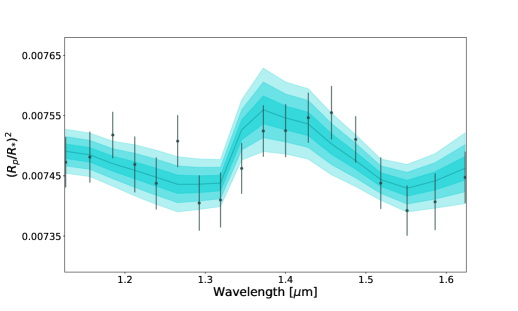
Figure 4: Best-fit transmission spectrum of WASP-117 b.

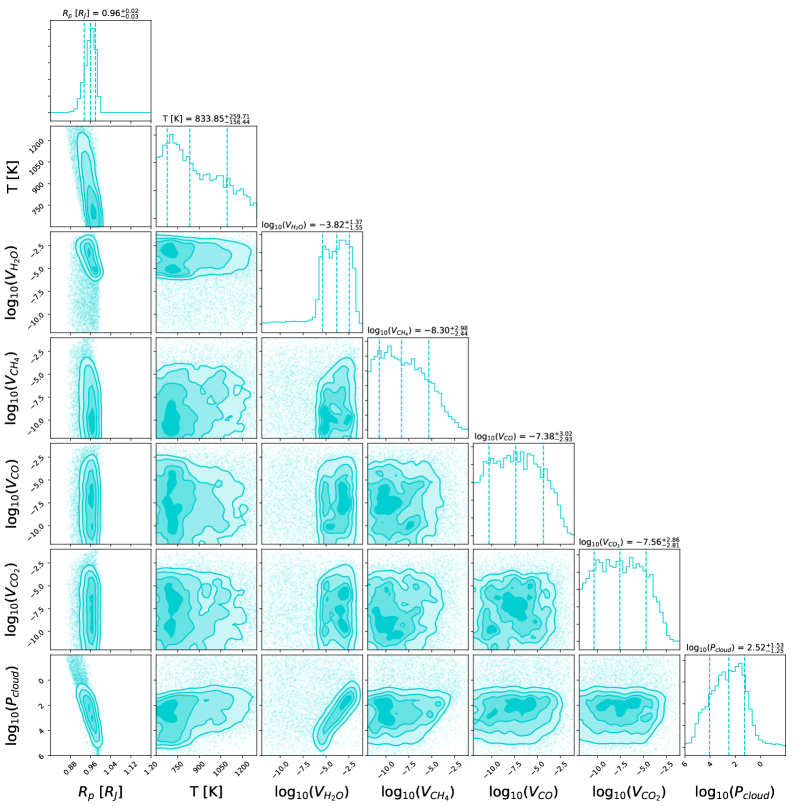
Figure 5: Posterior distributions for the transmission spectrum (see Figure 4) of WASP-117 b which indicate the presence of water vapour and cloud.

The abundance of water retrieved is consistent with results from population studies of gaseous planets such as Tsiaras et al. (2018), Pinhas et al. (2019) and Sing et al. (2016) and chemistry models of gaseous atmospheres (e.g. Venot et al. (2012)). While we did attempt to retrieve other trace gases such as CO, CH₄ and CO₂, we were unable to identify their presence. Our detected abundance of water vapor is consistent with a similar study of WASP-117 b, Carone et al. (2020), to within 1$\sigma$, however we find that the data do not constrain said abundance to great accuracy ($\log_{10}(V_{\text{H}_{2}\text{O}})$ at $1\sigma\in$ [-5.37, 2.45]). In addition we do not find evidence for the presence of other species, thus we are not able to adequately constrain atmospheric metallicity for this planet. The priors used in our retrieval run as well as the retrieved values are summarised in Table 3. The full posterior distribution for the parameters is shown in Figure 5. In the case of WASP-117 b, we detect our atmospheric retrieval signature at the ADI value of 2.30 which as in Kass & Raftery (1995) corresponds to positive evidence against the flatline model.

3.2 Ephemeris Refinement

The transits of WASP-117 b from HST and TESS were seen to arrive early compared to the predictions from Lendl et al. (2014). The ephemeris of WASP-117 b was recently refined by Mallonn et al. (2019). We used the observations from Mallonn et al. (2019), the original ephemeris from Lendl et al. (2014), and the new data analysed here to update the period and transit time for the planet. Using this data, we determined the ephemeris of WASP-117 b to be $P=10.0205928\pm 0.0000044$ days and $T_{0}$ = 2458688.251803 $\pm$ 0.000097 BJD_TDB where $P$ is the planet’s period, $T_{0}$ is the reference mid-time of the transit and BJD_TDB is the barycentric Julian date in the barycentric dynamical.

Our derived period is 1.2 s shorter than that from Mallonn et al. (2019). We improved the accuracy of the period and thus reduced the current uncertainty on the transit time with respect to the results from Mallonn et al. (2019). The observed minus calculated residuals, along with the fitted TESS light-curves are shown in Figure 6 while the fitted mid times can be found in Table 4. Our new observations have been uploaded to ExoClock, a coordinated follow-up programme to keep transit times up-to-date for the ESA Ariel mission.

Retrieval Analysis Parameters
Parameters	Prior bounds	Scale	Retrieved Value
$R_{p}$ [$R_{J}$]	[0.8, 2]	linear	0.96${}^{+0.02}_{-0.02}$
$T_{term}$ [K]	[600, 1300]	linear	833${}^{+260}_{-156}$
$V_{\text{H}_{2}\text{O}}$	[-12, -1]	$\log_{10}$	-3.82 ${}^{+1.37}_{-1.55}$
$V_{\text{CH}_{4}}$	[-12, -1]	$\log_{10}$	unconstrained
$V_{\text{CO}}$	[-12, -1]	$\log_{10}$	unconstrained
$V_{\text{CO}_{2}}$	[-12, -1]	$\log_{10}$	unconstrained
$P_{cloud}$	[6, -2]	$\log_{10}$	2.52 ${}^{+1.53}_{-1.25}$

Table 3: List of the retrieved parameters, their uniform prior bounds, the scaling used and the corresponding retrieved posterior distribution mean values.

Epoch	Transit Mid Time [BJDTDB]	Reference
-216	2456533.824040 $\pm$ 0.000950	Lendl et al. (2014)
-75	2457946.728100 $\pm$ 0.001980	Mallonn et al. (2019)
-74	2457956.749850 $\pm$ 0.001630	Mallonn et al. (2019)
-74	2457956.751130 $\pm$ 0.001050	Mallonn et al. (2019)
-34	2458357.571170 $\pm$ 0.000599	This Work†
-32	2458377.613147 $\pm$ 0.000456	This Work†
-31	2458387.633714 $\pm$ 0.000629	This Work†
-30	2458397.654772 $\pm$ 0.000588	This Work†
5	2458748.375370 $\pm$ 0.000082	This Work*
†Data from TESS *Data from Hubble

Table 4: Transit mid times used to refine the ephemeris of planets from this study.

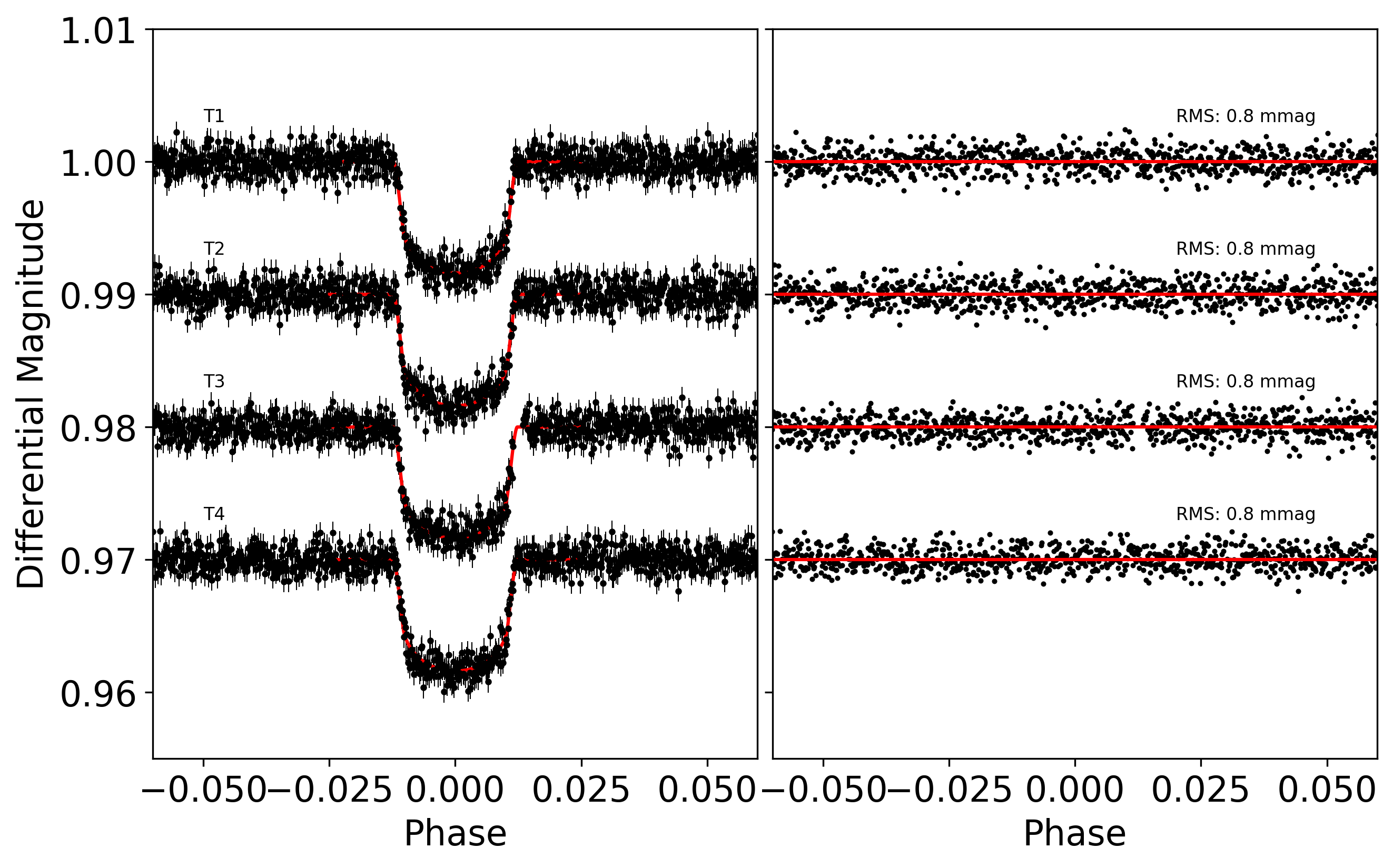
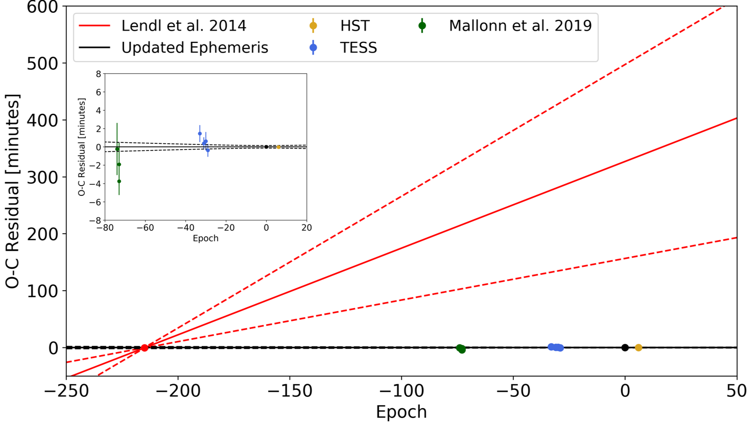
Figure 6: Top: TESS observations of WASP-117 b presented in this work. Left: detrended data and best-fit model. Right: residuals from fitting. Bottom: Observed minus calculated (O-C) mid-transit times for WASP-117 b. Transit mid time measurements from this work are shown in gold (HST) and blue (TESS), while the T₀ value for Lendl et al. (2014) is in red and the observations from Mallonn et al. (2019) are in green. The black line denotes the new ephemeris of this work with the dashed lines showing the associated 1$\sigma$ uncertainties and the black data point indicating the updated T₀. For comparison, the previous literature ephemeris and their 1$\sigma$ uncertainties are given in red. The inset figure shows a zoomed plot which highlights the precision of the TESS and HST mid time fits.

3.3 Ariel & JWST simulations

The ACE equilibrium chemistry package identified H₂O, CH₄, CO, CO₂ and NH₃ as the most relevant species in the atmosphere of WASP-117 b. Resulting abundance profiles for these chemical species, as a function of atmospheric pressure, are displayed in Figure 7, with the cooler-chemical atmosphere given by dashes, and the hotter-chemical atmosphere given by solid lines. The corresponding spectra created using these chemical profiles, but forward modelled using the retrieved terminator temperature of 833 K, as would be observed by Ariel and JWST, are displayed in Figure 8. We can see that in the cooler chemistry scenario, there is a distinctly larger abundance of CH₄ in the region [$10^{5},10^{2}]$ Pa, the observable region, compared with the hotter chemical regime.

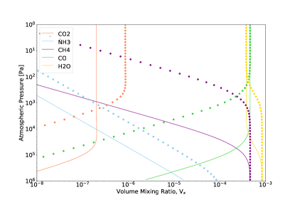
Figure 7: Equilibrium molecular abundance profiles as a function of atmospheric pressure for two different simulations of WASP-117 b’s atmosphere: dotted lines indicate cooler chemistry (800 K abundances); solid lines display hotter chemistry (1100 K abundances).

In order to further constrain the CH₄ abundances, retrieval analysis was carried out for these two sets of simulated spectra, akin to that described in Section 2.3. We used prior distributions as specified in Table 3, with the exception of a two-layer profile for CH₄, with a pressure threshold between the two chemical profile layers set to $10^{2}$ Pa for the 800 K atmospheres, and to $10^{3.5}$ Pa for the 1100 K ones. The retrieved methane abundances at the “surface”, at an atmospheric pressure larger than this threshold, and at the “top”, at pressures smaller than this are denoted as $\log_{10}(V_{\text{CH}_{4}})_{S}$ and $\log_{10}(V_{\text{CH}_{4}})_{T}$, respectively. The resulting posterior distributions for the parameters of both nominal atmospheres are over-plotted in Figures 9 and 10 for the Ariel and JWST spectra, respectively. Over-plotted onto the posterior graphs are “input” chemical abundance values; for the species where constant abundances have been assumed the value has been extracted from Figure 7 at $10^{3}$ Pa, whilst the values for the methane abundances in the surface and top layers are taken at pressure points one order of magnitude either side of the pressure inflection points, for both sets of atmospheres. Both Changeat et al. (2019) and Changeat et al. (2020) illustrate that the use of a 2-layer parameterisation, whilst significantly more revealing than an constant abundance profile, will only retrieve an abundance profile that aligns with the forward model at the peak of the molecular contribution function. Thus, our over-plotted abundance values are expected to be more accurate close to the pressure inflection points, but should be treated with caution at pressures elsewhere. Additionally, we note also that for the 1100 K atmospheres, molecular abundances prove harder to constrain but that forcing constant retrieval profiles on varied input abundance results in a bias on the retrieved temperature. This result is consistent with evidence for a retrieval bias towards lower determined temperatures than planetary effective temperatures, as investigated in MacDonald et al. (2020), Caldas et al. (2019) and Skaf et al. (2020).

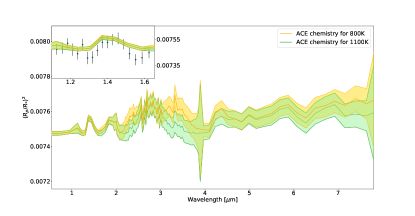
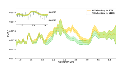
Figure 8: Simulated transmission spectra of WASP-117 b, as observed by Ariel with 15 transits (top) and JWST with 4 transits (bottom). Forward models generated using chemical equilibrium abundances for 800 K are shown in yellow, whilst that for 1100 K are shown in green; with both spectra simulated using the retrieval temperature $T_{term}=833$ K. Inset: zoom-in over the HST wavelength range with the observations over-plotted (not fitted).

Despite not being able to distinguish between the two regimes over the HST wavelength range, the distinction can in fact be made with 15 Ariel observations due to the CH₄ spectral features present due to ro-vibrational transitions at $2.3$, $3.3$ and $7.66\mu m$ (Yurchenko et al., 2014). As for JWST, only 4 transits (2 with NIRISS and 2 with NIRSpec G395M) are needed to illuminate this distinction. This makes WASP-117 b a very promising candidate for observations with both Ariel and JWST, as with its bright host star and posited chemistry, this Saturn-mass planet could further illuminate exoplanet atmospheric chemical dynamics.

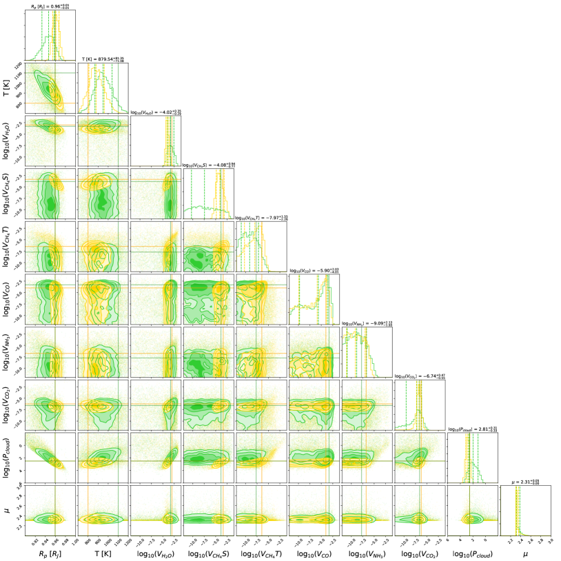
Figure 9: Posterior distributions over-plotted for a 2-layer retrieval of the simulated Ariel spectra given in Figure 8, with input from the 800 K and 1100 K atmospheres displayed in yellow and green, respectively. The posterior mean values presented correspond to the cooler atmospheric regime.

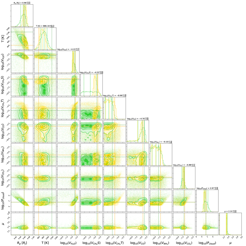
Figure 10: Posterior distributions over-plotted for a 2-layer retrieval of the simulated JWST spectra given in Figure 8, with input from the 800 K and 1100 K atmospheres displayed in yellow and green, respectively. The posterior mean values presented correspond to the cooler atmospheric regime.

4 Discussion

4.1 Retrieval Results and Atmospheric Temperature

Whilst the ADI of 2.30 provides positive but not strong evidence against the flat-line model, we recognise that this value is sensitive to the scattered region of the spectrum below $1.3\mu m.$ When the data points at 1.27$\mu m$ and 1.18$\mu m$ were removed and the same retrieval analysis performed, we obtain an ADI value of 4.30, moving over the threshold into strong evidence. The addition of WASP-117 b to the long list of gaseous planets with prominent water features (Tsiaras et al., 2018; Pinhas et al., 2019), solidifies further the evidence that water appears to be ubiquitous in the atmospheres of such planets, with the presence of clouds in fact obscuring water that sits deeper in the atmosphere, and so weakening the observed transmission spectral signal (Sing et al., 2016).

The terminator temperature was estimated to be $T_{term}=833^{+260}_{-156}$ K, which sits in the range [677 K, 1093 K] at the 1$\sigma$ level. Our retrieval analysis uses a temperature prior informed by equilibrium temperature arguments as outlined in Section 2.3. Although atmospheric parameters such as geometric albedo and heat redistribution are not well constrained for this planet, what is significant from a chemical perspective is the possible fluctuation of temperature around $\approx 900$ K between apastron and periastron, since this is the threshold for which CO-CH₄ conversion oscillates between CO or CH₄ dominant in the $10^{2}-10^{5}$ Pa visible-region of the atmosphere, as is observed in Visscher (2012) for solar-metallicity gas. We take $\beta=1$ and $A=0.3$ to derive an equilibrium temperature range of [816 K, 1116 K], whereas Lendl et al. (2014) take $\beta=1$ and $A=0$ finding [897 K, 1225 K]. Despite not agreeing exactly, both temperature ranges include 900 K.

We note that our retrieval analysis displays a significant degeneracy between the cloud pressure and water abundance. Degeneracies of this nature are common when only using data from WFC3 G141 (e.g. Tsiaras et al., 2018) and the addition of data spanning visible wavelengths has been shown to remove this (Pinhas et al., 2019). As TESS has also studied the transit of WASP-117 b it could provide additional information to constrain parameters. However, the transit depth recovered from the TESS data is extremely shallow, around 200 ppm lower than the WFC3 data-set. Carone et al. (2020) also found an anomalously low TESS transit depth.

Offsets between instruments can be caused for a number of reasons: due to imperfect correction of instrument systematics; from the use of different orbital parameters or limb darkening coefficients during the light curve fitting; or from stellar variability or activity (e.g. Stevenson et al., 2014a, b; Tsiaras et al., 2018; Alexoudi et al., 2018; Yip et al., 2019; Bruno et al., 2020; Pluriel et al., 2020; Murgas et al., 2020; Yip et al., submitted). Here, we fitted the data-sets with the same limb darkening laws and orbital parameters, ruling out that potential explanation. Carone et al. (2020) studied whether stellar activity or the transit light source effect could be causing this discrepancy and found, while some offset could be explained, the magnitude of the offset was too great for this alone to be the cause. Therefore, we anticipate the offset being due to imperfect correction of instrument systematics. In the white light curve (Figure 1) we noted the presence of some non-Gaussian residuals. While the divide-by-white method means the spectral light curves display Gaussian residuals, the whole spectrum may be shifted due to the imperfect white light curve fit. Further data, for example with the WFC3 G102 grism or CHEOPS, could help resolve this issue.

4.2 Atmospheric Chemistry

In order to understand the capabilities of future missions like JWST and Ariel to successfully probe the atmospheric chemistry of WASP-117 b it is paramount to consider the detection limits of various chemical species with respect to the resolution and wavelength coverage of their instruments. Our simulated atmospheres for WASP-117 b which we subsequently retrieve on are generated at the Ariel tier 2 resolution. The posterior distributions given in Figures 9 show that with 15 transits it is possible to reliably constrain the abundances of H₂O and of the carbon-based molecules CH₄ and CO₂, which is consistent with results from Changeat et al. (2020) in which upper atmosphere observational detection limits for tier 2 are determined to be $V_{x}\geq 10^{-7}$. For species like CO and NH₃, the detection limits are $V_{x}\geq 10^{-4}$, $10^{-7}$, respectively. Thus, in agreement with our simulations, it is clear that for Ariel, tracing these species will remain challenging. Correspondingly, simulated JWST spectra for 4 transits enable tighter constraints to be made upon retrieving, as illustrated in Figure 10, but giving the same overall conclusions on detectability. In order to unify the power of both missions, but to avoid the well-known issues related to combining data-sets from different instruments as described in Section 4.1, results from each instrument should be used as prior knowledge to inform analysis with the other. For example, since the wavelength coverage of Ariel reaches as far into the visible as 0.5 $\mu$m, and further than JWST at 0.6 $\mu$m, these few additional data points could aid the removal of the degeneracy between retrieved cloud layer pressure and water vapour abundance. Additionally, as JWST has a greater sensitivity across the 3.0-3.5 $\mu m$ region, where the models are most distinctly separated, the NIRSpec G395M observations could be complementary to the Ariel data. As we have discussed, eccentric orbits cause a variation of atmospheric temperature due to variations in levels of stellar flux received by the planet as it traverses its orbit. As a result we can expect atmospheric chemical profiles to vary with time. A schematic diagram for the orbit of WASP-117 b’s orbit is displayed in Figure 3, with the line-of-sight direction for which we observe the system during transit highlighted in yellow. In order to assess the chemistry that is observable during transit, chemical and dynamical mixing timescales must be considered with respect to the planet’s orbital and spin periods. Visscher (2012) asserts that eccentric planet atmospheric chemistry is only affected by vertical mixing if the time elapsed between apastron and periastron exceeds vertical mixing timescales ($\tau_{mix}<\frac{1}{2}P_{orbital}$). Thus if, for now, we make the assumption that vertical mixing timescales are slower than this threshold, we can compare chemical timescales $\tau_{chem}(x)$ for a given molecular species $x$ to orbital timescales to assess what sort of chemistry might be observable during transit.

These chemical timescales are functions of pressure and temperature and so will oscillate throughout orbit; allowing perhaps for warmer chemistry to remain visible as the planet enters transit, despite the proximity of its point of ingress to apastron. As the temperature reaches 838 K at transit, the time taken to reach chemical equilibrium corresponding to this new atmospheric temperature may be larger than the time taken to travel there from periastron and thus the chemistry may not be able to adapt to the changes in the irradiation environment. Visscher (2012) calculates chemical timescales for various species in the atmospheres of the eccentric gaseous giant exoplanets HAT-P-2 b and CoRoT-10 b. In particular, they obtain $\tau_{chem}(\text{CH}_{4})\approx\tau_{chem}(\text{CO})\approx 10^{20}$ s in the observable region of $10^{2}-10^{5}$ Pa, with respect to CH₄-CO inter-conversion, at WASP-117 b’s equilibrium periastron temperature of 838 K, which is indeed larger than half the planet’s orbital period of around $10^{5}$ s.

However, so far this argument only considers chemical equilibrium processes, which is almost certainly a gross simplification. In order to constrain chemical timescales more rigorously, a more in-depth analysis of the atmosphere which includes photo-dissociation processes, disequilibrium chemistry and vertical and horizontal mixing processes is required. However, in order to carry out preliminary analysis, we neglect vertical mixing, assume either tidal locking or a spin-synchronous orbit and consider only equilibrium chemical processes as a first-order approximation to assess feasibility of detectability. Under these assumptions we are left with two extremes for observable chemistry during transit. Assuming thermo-chemical equilibrium is achieved at periastron we may observe warmer periastron (1100 K) chemistry if the chemical timescales are slow enough such that the chemistry does not have time to adapt to the decreased temperature by the time it enters transit close to apastron ($\tau_{chem}>\frac{1}{2}P_{orbital}$). Or, on the contrary, if chemical timescales are fast enough to allow for the chemistry to adapt to the apastron temperature close to transit ($\tau_{chem}<\frac{1}{2}P_{orbital}$), or if chemical timescales are slow but chemical equilibrium is reached at apastron, we may observe cooler (800 K) apastron chemistry, i.e. what we expect.

A further caveat to this is that in the likely case that the planet spins, spin-orbit resonance may be able to somewhat homogenise the warmer and cooler regimes ($\tau_{mix}>P_{spin}$) possibly giving the planet a globally averaged chemistry between the hotter and cooler cases. In addition to the aforementioned chemical assumptions, other caveats to such a simplified analysis include the lack of a 3D atmospheric model, with self-consistent dynamics. Caldas et al. (2019) illustrate that 3D analysis could enable the capture of the contamination of the terminator by the day-side of the planet, due to strong irradiation at the day-side, whilst MacDonald et al. (2020) show that 1D retrieval analyses cannot capture compositional differences between the morning and evening terminator, whilst both effects could result in chemical inhomogeneities in the terminator region. A comprehensive study of all such processes would enable accurate characterisation of WASP-117 b’s atmospheric chemistry, with the presented analysis of the two extremes of equilibrium chemistry serving to motivate follow-up study and observation.

5 Conclusion

WASP-117 b’s possession of an eccentric and misaligned orbit around its bright and stable F9 host makes it a tantalising object for atmospheric characterisation, since chemical timescales for CH₄ compete with the orbital period. With HST WFC3 observations, we present a retrieval solution with a well-constrained water vapour volume mixing ratio of $\log_{10}(V_{\text{H}_{2}\text{O}})=-3.82^{+1.37}_{-1.55}$, alongside a layer of opaque cloud. Carbon-based molecules such as CO, CO₂ and CH₄ prove harder to constrain using such data as the wavelength coverage and the signal-to-noise remains limiting. With the future telescopes JWST and Ariel, we present simulated spectra for WASP-117 b as would be observed by these missions and show that it should be possible to probe possible variations in CH₄ chemistry in the observable region of the atmosphere.

References

- Abel et al. (2011) Abel, M., Frommhold, L., Li, X., & Hunt, K. L. 2011, The Journal of Physical Chemistry A, 115, 6805
- Abel et al. (2012) —. 2012, The Journal of chemical physics, 136, 044319
- Agúndez et al. (2012) Agúndez, M., Venot, O., Iro, N., et al. 2012, Astronomy & Astrophysics, 548, A73. http://dx.doi.org/10.1051/0004-6361/201220365
- Al-Refaie et al. (2019) Al-Refaie, A. F., Changeat, Q., Waldmann, I. P., & Tinetti, G. 2019, arXiv e-prints, arXiv:1912.07759
- Alexoudi et al. (2018) Alexoudi, X., Mallonn, M., von Essen, C., et al. 2018, A&A, 620, A142
- Anderson et al. (2014) Anderson, D. R., Collier Cameron, A., Delrez, L., et al. 2014, Monthly Notices of the Royal Astronomical Society, 445, 1114–1129. http://dx.doi.org/10.1093/mnras/stu1737
- Astropy Collaboration et al. (2018) Astropy Collaboration, Price-Whelan, A. M., Sipőcz, B. M., et al. 2018, AJ, 156, 123
- Benneke et al. (2019) Benneke, B., Wong, I., Piaulet, C., et al. 2019, arXiv e-prints, arXiv:1909.04642
- Brogi et al. (2012) Brogi, M., Snellen, I. A. G., de Kok, R. J., et al. 2012, Nature, 486, 502–504. http://dx.doi.org/10.1038/nature11161
- Bruno et al. (2020) Bruno, G., Lewis, N. K., Alam, M. K., et al. 2020, MNRAS, 491, 5361
- Caldas et al. (2019) Caldas, A., Leconte, J., Selsis, F., et al. 2019, Astronomy & Astrophysics, 623, A161. http://dx.doi.org/10.1051/0004-6361/201834384
- Carone (2017) Carone, L. 2017, Now you see me - the WASP-117b version, HST Proposal, ,
- Carone et al. (2020) Carone, L., Mollière, P., Zhou, Y., et al. 2020, arXiv e-prints, arXiv:2006.05382
- Changeat et al. (2020) Changeat, Q., Al-Refaie, A., Mugnai, L. V., et al. 2020, AJ, 160, 80
- Changeat et al. (2019) Changeat, Q., Edwards, B., Waldmann, I. P., & Tinetti, G. 2019, The Astrophysical Journal, 886, 39. http://dx.doi.org/10.3847/1538-4357/ab4a14
- Claret et al. (2012) Claret, A., Hauschildt, P. H., & Witte, S. 2012, A&A, 546, A14
- Claret et al. (2013) —. 2013, A&A, 552, A16
- Collette (2013) Collette, A. 2013, Python and HDF5 (O’Reilly)
- Cowan et al. (2015) Cowan, N. B., Greene, T., Angerhausen, D., et al. 2015, Publications of the Astronomical Society of the Pacific, 127, 311
- de Wit et al. (2018) de Wit, J., Wakeford, H. R., Lewis, N. K., et al. 2018, Nature Astronomy, 2, 214–219. http://dx.doi.org/10.1038/s41550-017-0374-z
- Demangeon et al. (2018) Demangeon, O. D. S., Faedi, F., Hébrard, G., et al. 2018, Astronomy & Astrophysics, 610, A63. http://dx.doi.org/10.1051/0004-6361/201731735
- Deming et al. (2013) Deming, D., Wilkins, A., McCullough, P., et al. 2013, The Astrophysical Journal, 774, 95. http://dx.doi.org/10.1088/0004-637X/774/2/95
- Demory et al. (2016) Demory, B.-O., Gillon, M., de Wit, J., et al. 2016, Nature, 532, 207–209. http://dx.doi.org/10.1038/nature17169
- Edwards et al. (2020) Edwards, B., Al-Refaie, A., Lagage, P., & Gastaud, R. 2020, in prep
- Edwards et al. (2019) Edwards, B., Mugnai, L., Tinetti, G., Pascale, E., & Sarkar, S. 2019, The Astronomical Journal, 157, 242
- Edwards et al. (2020a) Edwards, B., Changeat, Q., Baeyens, R., et al. 2020a, AJ, 160, 8
- Edwards et al. (2020b) Edwards, B., Changeat, Q., Yip, K. H., et al. 2020b, MNRAS, doi:10.1093/mnras/staa1245
- Evans et al. (2017) Evans, T. M., Sing, D. K., Kataria, T., et al. 2017, Nature, 548, 58–61. http://dx.doi.org/10.1038/nature23266
- Feroz et al. (2009) Feroz, F., Hobson, M. P., & Bridges, M. 2009, MNRAS, 398, 1601
- Fletcher et al. (2018) Fletcher, L. N., Gustafsson, M., & Orton, G. S. 2018, The Astrophysical Journal Supplement Series, 235, 24
- Foreman-Mackey (2016) Foreman-Mackey, D. 2016, The Journal of Open Source Software, 1, 24. https://doi.org/10.21105/joss.00024
- Foreman-Mackey et al. (2013) Foreman-Mackey, D., Hogg, D. W., Lang, D., & Goodman, J. 2013, PASP, 125, 306
- Fraine et al. (2014) Fraine, J., Deming, D., Benneke, B., et al. 2014, Nature, 513, 526–529. http://dx.doi.org/10.1038/nature13785
- Gordon et al. (2016) Gordon, I., Rothman, L. S., Wilzewski, J. S., et al. 2016, in AAS/Division for Planetary Sciences Meeting Abstracts, Vol. 48, AAS/Division for Planetary Sciences Meeting Abstracts #48, 421.13
- Greene et al. (2016) Greene, T. P., Line, M. R., Montero, C., et al. 2016, The Astrophysical Journal, 817, 17. http://dx.doi.org/10.3847/0004-637X/817/1/17
- Hartman et al. (2010) Hartman, J. D., Bakos, G. A., Sato, B., et al. 2010, The Astrophysical Journal, 726, 52. http://dx.doi.org/10.1088/0004-637X/726/1/52
- Hartman et al. (2015) Hartman, J. D., Bhatti, W., Bakos, G. A., et al. 2015, The Astronomical Journal, 150, 168. http://dx.doi.org/10.1088/0004-6256/150/6/168
- Hunter (2007) Hunter, J. D. 2007, Computing in Science & Engineering, 9, 90
- Hébrard et al. (2014) Hébrard, G., Santerne, A., Montagnier, G., et al. 2014, Astronomy & Astrophysics, 572, A93. http://dx.doi.org/10.1051/0004-6361/201424268
- Iyer et al. (2016) Iyer, A. R., Swain, M. R., Zellem, R. T., et al. 2016, ApJ, 823, 109
- Jenkins et al. (2016) Jenkins, J. M., Twicken, J. D., McCauliff, S., et al. 2016, in Society of Photo-Optical Instrumentation Engineers (SPIE) Conference Series, Vol. 9913, Proc. SPIE, 99133E
- Kass & Raftery (1995) Kass, R. E., & Raftery, A. E. 1995, Journal of the american statistical association, 90, 773
- Kreidberg et al. (2014) Kreidberg, L., Bean, J. L., Désert, J.-M., et al. 2014, Nature, 505, 69
- Kreidberg et al. (2019) Kreidberg, L., Koll, D. D. B., Morley, C., et al. 2019, Nature, 573, 87–90. http://dx.doi.org/10.1038/s41586-019-1497-4
- Laughlin et al. (2009) Laughlin, G., Deming, D., Langton, J., et al. 2009, Nature, 457, 562. https://doi.org/10.1038/nature07649
- Lendl et al. (2014) Lendl, M., Triaud, A. H. M. J., Anderson, D. R., et al. 2014, A&A, 568, A81
- Li et al. (2015) Li, G., Gordon, I. E., Rothman, L. S., et al. 2015, The Astrophysical Journal Supplement Series, 216, 15
- Linsky et al. (2010) Linsky, J. L., Yang, H., France, K., et al. 2010, The Astrophysical Journal, 717, 1291–1299. http://dx.doi.org/10.1088/0004-637X/717/2/1291
- MacDonald et al. (2020) MacDonald, R. J., Goyal, J. M., & Lewis, N. K. 2020, Why is it so Cold in Here?: Explaining the Cold Temperatures Retrieved from Transmission Spectra of Exoplanet Atmospheres, , , arXiv:2003.11548
- Macintosh et al. (2015) Macintosh, B., Graham, J. R., Barman, T., et al. 2015, Science, 350, 64–67. http://dx.doi.org/10.1126/science.aac5891
- Majeau et al. (2012) Majeau, C., Agol, E., & Cowan, N. B. 2012, The Astrophysical Journal, 747, L20. http://dx.doi.org/10.1088/2041-8205/747/2/L20
- Mallonn et al. (2019) Mallonn, M., von Essen, C., Herrero, E., et al. 2019, A&A, 622, A81
- McKinney (2011) McKinney, W. 2011, Python for High Performance and Scientific Computing, 14
- Méndez & Rivera-Valentín (2017) Méndez, A., & Rivera-Valentín, E. G. 2017, ApJ, 837, L1
- Morello et al. (2020) Morello, G., Claret, A., Martin-Lagarde, M., et al. 2020, AJ, 159, 75
- Morello et al. (2016) Morello, G., Waldmann, I. P., & Tinetti, G. 2016, The Astrophysical Journal, 820, 86. http://dx.doi.org/10.3847/0004-637X/820/2/86
- Mugnai et al. (2020) Mugnai, L. V., Pascale, E., Edwards, B., Papageorgiou, A., & Sarkar, S. 2020, arXiv e-prints, arXiv:2009.07824
- Murgas et al. (2020) Murgas, F., Chen, G., Nortmann, L., Pallé, E., & Nowak, G. 2020, arXiv e-prints, arXiv:2007.02741
- Oliphant (2006) Oliphant, T. E. 2006, A guide to NumPy, Vol. 1 (Trelgol Publishing USA)
- Peek et al. (2019) Peek, J., Desai, V., White, R. L., et al. 2019, in BAAS, Vol. 51, 105
- Pinhas et al. (2019) Pinhas, A., Madhusudhan, N., Gandhi, S., & MacDonald, R. 2019, MNRAS, 482, 1485
- Pluriel et al. (2020) Pluriel, W., Whiteford, N., Edwards, B., et al. 2020, AJ, 160, 112
- Polyansky et al. (2018) Polyansky, O. L., Kyuberis, A. A., Zobov, N. F., et al. 2018, Monthly Notices of the Royal Astronomical Society, 480, 2597
- Ricker et al. (2014) Ricker, G. R., Winn, J. N., Vanderspek, R., et al. 2014, in Proceedings of the SPIE, Vol. 9143, Space Telescopes and Instrumentation 2014: Optical, Infrared, and Millimeter Wave, 914320
- Rothman et al. (2010) Rothman, L., Gordon, I., Barber, R., et al. 2010, Journal of Quantitative Spectroscopy and Radiative Transfer, 111, 2139
- Rothman & Gordon (2014) Rothman, L. S., & Gordon, I. E. 2014, in 13th International HITRAN Conference, June 2014, Cambridge, Massachusetts, USA
- Sing et al. (2016) Sing, D. K., Fortney, J. J., Nikolov, N., et al. 2016, Nature, 529, 59
- Skaf et al. (2020) Skaf, N., Bieger, M. F., Edwards, B., et al. 2020, AJ, 160, 109
- Smith et al. (2012) Smith, J. C., Stumpe, M. C., Van Cleve, J. E., et al. 2012, PASP, 124, 1000
- Stevenson et al. (2014a) Stevenson, K. B., Bean, J. L., Fabrycky, D., & Kreidberg, L. 2014a, The Astrophysical Journal, 796, 32
- Stevenson et al. (2014b) Stevenson, K. B., Bean, J. L., Seifahrt, A., et al. 2014b, The Astronomical Journal, 147, 161
- Stevenson et al. (2014c) Stevenson, K. B., Desert, J.-M., Line, M. R., et al. 2014c, Science, 346, 838–841. http://dx.doi.org/10.1126/science.1256758
- Stumpe et al. (2014) Stumpe, M. C., Smith, J. C., Catanzarite, J. H., et al. 2014, PASP, 126, 100
- Stumpe et al. (2012) Stumpe, M. C., Smith, J. C., Van Cleve, J. E., et al. 2012, PASP, 124, 985
- Swain et al. (2008) Swain, M. R., Vasisht, G., Tinetti, G., et al. 2008, Molecular Signatures in the Near Infrared Dayside Spectrum of HD 189733b, , , arXiv:0812.1844
- Tennyson et al. (2016) Tennyson, J., Yurchenko, S. N., Al-Refaie, A. F., et al. 2016, Journal of Molecular Spectroscopy, 327, 73 , new Visions of Spectroscopic Databases, Volume II. http://www.sciencedirect.com/science/article/pii/S0022285216300807
- Tinetti et al. (2010) Tinetti, G., Deroo, P., Swain, M. R., et al. 2010, The Astrophysical Journal, 712, L139–L142. http://dx.doi.org/10.1088/2041-8205/712/2/L139
- Tinetti et al. (2018) Tinetti, G., Drossart, P., Eccleston, P., et al. 2018, Experimental Astronomy. https://doi.org/10.1007/s10686-018-9598-x
- Trifonov et al. (2018) Trifonov, T., Kürster, M., Zechmeister, M., et al. 2018, Astronomy & Astrophysics, 609, A117. http://dx.doi.org/10.1051/0004-6361/201731442
- Tsiaras et al. (2016a) Tsiaras, A., Waldmann, I., Rocchetto, M., et al. 2016a, ascl:1612.018
- Tsiaras et al. (2016b) Tsiaras, A., Waldmann, I. P., Rocchetto, M., et al. 2016b, ApJ, 832, 202
- Tsiaras et al. (2019) Tsiaras, A., Waldmann, I. P., Tinetti, G., Tennyson, J., & Yurchenko, S. N. 2019, Nature Astronomy, doi:10.1038/s41550-019-0878-9
- Tsiaras et al. (2016c) Tsiaras, A., Rocchetto, M., Waldmann, I. P., et al. 2016c, ApJ, 820, 99
- Tsiaras et al. (2018) Tsiaras, A., Waldmann, I. P., Zingales, T., et al. 2018, AJ, 155, 156
- Venot et al. (2012) Venot, O., Hébrard, E., Agúndez, M., et al. 2012, Astronomy & Astrophysics, 546, A43. http://dx.doi.org/10.1051/0004-6361/201219310
- Vidal-Madjar et al. (2003) Vidal-Madjar, A., Lecavelier des Etangs, A., Désert, J.-M., et al. 2003, Nature, 422, 143
- Virtanen et al. (2020) Virtanen, P., Gommers, R., Oliphant, T. E., et al. 2020, Nature Methods, 17, 261
- Visscher (2012) Visscher, C. 2012, The Astrophysical Journal, 757, 5. http://dx.doi.org/10.1088/0004-637X/757/1/5
- Waldmann et al. (2015a) Waldmann, I. P., Rocchetto, M., Tinetti, G., et al. 2015a, ApJ, 813, 13
- Waldmann et al. (2015b) Waldmann, I. P., Tinetti, G., Rocchetto, M., et al. 2015b, ApJ, 802, 107
- Yip et al. (submitted) Yip, K. H., Changeat, Q., Edwards, B., et al. submitted
- Yip et al. (2019) Yip, K. H., Waldmann, I. P., Tsiaras, A., & Tinetti, G. 2019, arXiv e-prints, arXiv:1811.04686
- Yurchenko & Tennyson (2014) Yurchenko, S. N., & Tennyson, J. 2014, Monthly Notices of the Royal Astronomical Society, 440, 1649
- Yurchenko et al. (2014) Yurchenko, S. N., Tennyson, J., Bailey, J., Hollis, M. D. J., & Tinetti, G. 2014, Proceedings of the National Academy of Sciences, 111, 9379–9383. http://dx.doi.org/10.1073/pnas.1324219111