High-accuracy calculation of the deuteron charge and quadrupole form factors in chiral effective field theory

Abstract

We present a comprehensive analysis of the deuteron charge and quadrupole form factors based on the latest two-nucleon potentials and charge density operators derived in chiral effective field theory. The single- and two-nucleon contributions to the charge density are expressed in terms of the proton and neutron form factors, for which the most up-to-date empirical parametrizations are employed. By adjusting the fifth-order short-range terms in the two-nucleon charge density operator to reproduce the world data on the momentum-transfer dependence of the deuteron charge and quadrupole form factors, we predict the values of the structure radius and the quadrupole moment of the deuteron: $r_{\rm str}=1.9729\begin{subarray}{c}+0.0015\\ -0.0012\end{subarray}\ \text{fm},\ Q_{d}=0.2854\begin{subarray}{c}+0.0038\\ -0.0017\end{subarray}\ \text{fm}^{2}.$ A comprehensive and systematic analysis of various sources of uncertainty in our predictions is performed. Following the strategy advocated in our recent publication Phys. Rev. Lett. 124, 082501 (2020), we employ the extracted structure radius together with the accurate atomic data for the deuteron-proton mean-square charge radii difference to update the determination of the neutron charge radius, for which we find: $r_{n}^{2}=-0.105\begin{subarray}{c}+0.005\\ -0.006\end{subarray}\,\text{fm}^{2}$. Given the observed rapid convergence of the deuteron form factors in the momentum-transfer range of $Q\simeq 1-2.5$ fm^-1, we argue that this intermediate-energy domain is particularly sensitive to the details of the nucleon form factors and can be used to test different parametrizations.

I Introduction

Chiral effective field theory (EFT) is becoming a precision tool for analyzing low-energy few-nucleon reactions and nuclear structure Epelbaum:2008ga ; Epelbaum:2012vx ; Epelbaum:2019kcf ; Machleidt:2011zz . The chiral expansion of the nucleon-nucleon (NN) force has been recently pushed to fifth order (N⁴LO) Entem:2014msa and even beyond Entem:2015xwa . The last-generation chiral EFT NN potentials of Ref. Reinert:2017usi provide an excellent description of the neutron-proton and proton-proton scattering data, which, at the highest considered order, is even better than the one achieved using so-called high-precision phenomenological potentials such as the CD Bonn Machleidt:2000ge , Nijm I, II and Reid93 Stoks:1994wp and AV18 Wiringa:1994wb models. The essential feature of these chiral NN forces is the usage of a semi-local regulator Epelbaum:2014efa ; Epelbaum:2014sza , see also Refs. Gezerlis:2013ipa ; Piarulli:2014bda , which allows one to significantly reduce the amount of finite-cutoff artifacts in the long-range part of the interaction. For an alternative regularization approach using a non-local cutoff see Ref. Entem:2017gor . The chiral NN potentials of Ref. Reinert:2017usi also provide a clear evidence of the two-pion exchange, which is determined in a parameter-free way by the chiral symmetry of QCD along with the empirical information on pion-nucleon scattering from the recent analysis in the framework of the Roy-Steiner equations Hoferichter:2015tha ; Hoferichter:2015hva . In the most recent work of Ref. Reinert:2020mcu , the potential of Ref. Reinert:2017usi was updated to include also the charge-independence-breaking and charge-symmetry-breaking NN interactions up through N⁴LO.

In parallel with these studies, a simple and universal algorithm for quantifying truncation errors in chiral EFT without reliance on cutoff variation was formulated in Ref. Epelbaum:2014efa and validated in Ref. Epelbaum:2014sza . This approach has been successfully applied to a variety of low-energy hadronic observables, see e.g. Refs. Binder:2015mbz ; Binder:2018pgl ; Epelbaum:2018ogq ; Skibinski:2016dve ; Yao:2016vbz ; Siemens:2017opr ; Lynn:2019vwp ; NevoDinur:2018hdo ; Blin:2018pmj ; Lonardoni:2018nob . In Refs. Furnstahl:2015rha ; Melendez:2017phj ; Wesolowski:2018lzj ; Epelbaum:2019zqc , it was re-interpreted and further scrutinized within a Bayesian approach.

These developments provide a solid basis for applications beyond the two-nucleon system and offer highly nontrivial possibilities to test chiral EFT by pushing the expansion to high orders. In this paper, we focus on the charge and quadrupole elastic form factors (FFs) of the deuteron.

The electromagnetic FFs of the deuteron certainly belong to the most extensively studied observables in nuclear physics, see Refs. Garcon:2001sz ; Gilman:2001yh ; Marcucci:2015rca for review articles. A large variety of theoretical approaches ranging from non-relativistic quantum mechanics to fully covariant models have been applied to this problem since the 1960s, see Ref. Phillips:2003pa for an overview. The electromagnetic structure of the deuteron has also been investigated in the framework of pionless Chen:1999tn and chiral Phillips:1999am ; Walzl:2001vb ; Phillips:2003jz ; Phillips:2006im ; Valderrama:2007ja ; Piarulli:2012bn ; Epelbaum:2013naa EFT.

In spite of the extensive existing theoretical work, there is a strong motivation to take a fresh look at the deuteron FFs in the framework of chiral EFT. First of all, the calculation of the deuteron charge FF with unprecedented accuracy, by employing consistent NN interactions and charge density operators up to the fifth order in the chiral expansion, provides direct access to the structure radius of the deuteron and through that to the neutron charge radius, as elaborated in Ref. Filin:2019eoe . Similarly, the quantitative description of the quadrupole FF, supplemented with the comprehensive error analysis, opens the possibility to extract the quadrupole moment of the deuteron that is known very accurately and thus probes our understanding of the nuclear forces and currents. In this context, it is worth mentioning the tendency of modern nuclear interactions derived in chiral EFT to significantly underpredict the radii of medium-mass and heavy nuclei, see e.g. Cipollone:2014hfa . The existing calculations for $A\geq 16$ systems do, however, not take into account contributions to the three-nucleon force beyond third order of the chiral expansion (N²LO), exchange currents and relativistic corrections and also suffer from uncertainties intrinsic to truncations of the many-body Hilbert space. It is, therefore, of great importance to test the role of these effects in consistent calculations of electromagnetic few-nucleon processes at high orders in chiral EFT along with a careful error analysis. Focusing on the few-nucleon sector has an advantage of avoiding potential uncertainties associated with many-body methods. In particular, no additional softening of the interactions by using e.g. Similarity Renormalization Group transformation Bogner:2007rx is necessary for the light nuclei like ²H, ³H, ³He and ⁴He. It is also interesting and important to test the performance and applicability range of the newest high-precision chiral NN potentials of Refs. Reinert:2020mcu ; Reinert:2017usi and the charge density operators by studying the momentum-transfer ($Q$) dependence of the deuteron FFs and their convergence with respect to the chiral expansion. This provides a rather non-trivial test of the applicability range of chiral EFT since the deuteron FFs decrease by several orders of magnitude with increasing values of $Q$. Therefore, a correction to the charge operator that is small at $Q^{2}=0$ may, potentially, have a large impact at higher-$Q^{2}$ values.

In this paper, we perform a detailed analysis of the deuteron charge and quadrupole FFs in chiral EFT. We include all contributions to the charge-density operator at fourth order (N³LO) relative to the leading single-nucleon operator and take into account the short-range operators at N⁴LO. The strength of the N⁴LO short-range operators is adjusted to obtain the best fits to the experimental data for the deuteron charge and quadrupole FFs. We demonstrate that both the single- and two-nucleon charge density operators can be expressed in terms of the nucleon FFs and exploit this fact in the calculation of the deuteron FFs. This allows us to avoid reliance on the strict chiral expansion for the nucleon FFs by employing the corresponding empirical parametrizations. Since the errors related to the truncation of the chiral expansion are still very small in the momentum range of $Q\simeq 1-2.5$ fm^-1, this intermediate energy domain appears to be particularly sensitive to the nucleon FFs and thus can be used to test the consistency of the employed up-to-date nucleon FFs with the deuteron FFs.

Once the two NN contact terms in the charge density operator are determined from a fit to the world data on the deuteron FFs, we arrive at a parameter-free prediction for the quantities at $Q=0$, namely the structure radius and the quadrupole moment of the deuteron. It is worth mentioning that the nucleon FFs do not contribute to the extracted deuteron observables at $Q=0$. We perform various consistency checks of our theoretical approach and demonstrate that (i) our results show only a mild residual cutoff dependence; (ii) the results for the deuteron FFs, the structure radius and the quadrupole moment are basically insensitive to the choice of off-shell parameters entering the NN potentials and the charge density operator. However, this is only true as long as the NN potentials and the charge density are calculated consistently, which implies that the nucleon FFs must be included both in the one and two-body charge density operators, as advocated below. Finally, we perform a detailed error analysis of the obtained results by addressing various sources of uncertainties.

In Ref. Filin:2019eoe , we already employed this approach to extract the structure radius from the charge deuteron FF. Here, we provide additional details of the calculation and update the analysis of Ref. Filin:2019eoe in the following aspects: (a) we employ the latest version of the NN potential from Ref. Reinert:2020mcu that includes the relevant isospin breaking corrections, (ii) we carry out a combined analysis of both the charge and quadrupole deuteron FFs, (iii) relying on our Bayesian estimate of the truncation error from the chiral expansion, in the fits to the FF data we extend the momentum range to $Q\sim 6$ fm^-1 as compared to $Q\sim 4$ fm^-1 used in Ref. Filin:2019eoe .

Our paper is organized as follows. In Section II, we discuss a general formalism to calculate the form factors of the deuteron. Sections III and IV are devoted to the chiral expansion and regularization of the charge density operator. In Section III we also give a short overview of the nucleon FFs used as input in our calculations. Section V deals with the treatment of the relativistic corrections. Next, the notation for various contributions to the form factors, their chiral order and relations to the structure radius and the quadrupole moment are specified in Section VI. Our results for the momentum-transfer dependence of the charge and quadrupole FFs are presented in Section VII. After fixing the short-range charge density operator from the best fit to the experimental data we extract the values of the deuteron structure radius, the neutron charge radius and the deuteron quadrupole moment and analyze various sources of uncertainties. Also, we discuss the convergence of the chiral expansion for both the deuteron FFs and the extracted quantities at $Q=0$. The main results of our study are summarized in Section VIII, where we also discuss their impact on the determination of the neutron charge radius using high-accuracy atomic data on the deuteron-proton charge radius difference.

II Formalism

II.1 Elastic electron-deuteron scattering

The kinematics of elastic electron-deuteron scattering is visualized in Fig. 1 (a) and can be defined as

$$d(P,\lambda_{d})+e^{-}(p_{e},\nu)\;\to\;d(P^{\prime},\lambda_{d}^{\prime})+e^{-}(p_{e}^{\prime},\nu^{\prime}),$$ (1)

where variables in brackets denote the momentum and spin projection of the corresponding particle.

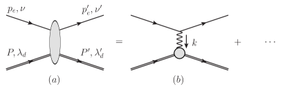
Figure 1: Diagrams representing elastic electron-deuteron scattering. Diagram (a) shows a general contribution to the elastic electron-deuteron scattering process and the corresponding kinematics. Diagram (b) visualizes the one-photon-exchange contribution, while the ellipses refer to multi-photon-exchange processes suppressed by powers of the fine structure constant. Single, double and wiggly lines correspond to electrons, deuterons, and photons respectively.

Throughout this work, we focus on the one-photon-exchange mechanism, see Fig. 1 (b), which provides a direct relation between the electron-deuteron scattering observables and the deuteron form factors. Each additional photon exchange is suppressed by one power of the fine-structure constant. Thus, in line with the conclusions of Ref. Dong:2009zzc , these corrections will be neglected below — see Sec. II.5 for a more detailed discussion. The one-photon-exchange amplitude of elastic electron-deuteron scattering, see Fig. 1 (b), can be factorized into leptonic and hadronic parts Arnold:1979cg :

$$\mathcal{M}=e\bar{u}(p_{e}^{\prime},\nu^{\prime})\gamma_{\mu}u(p_{e},\nu)\frac{1}{k^{2}}\Braket{P^{\prime},\lambda_{d}^{\prime}}{J^{\mu}}{P,\lambda_{d}},$$ (2)

where $e$ is the magnitude of the electron charge, $u$ and $\bar{u}$ are the spinors of the initial and final electrons normalized as $\bar{u}(p,\nu)u(p,\nu)=2m_{e}$ with $m_{e}$ being the electron mass, $\gamma_{\mu}$ are the Dirac matrices and $k=P^{\prime}-P$ is the four-momentum of the exchanged photon. For convenience, we define a quantity $Q^{2}$, which is positive in the space-like region, and the corresponding dimensionless variable $\eta$ via

$$Q^{2}:=-k_{\mu}k^{\mu}=-k^{2}=-{(P^{\prime}-P)}^{2}\geq 0,\qquad\eta:=\frac{Q^{2}}{4m_{d}^{2}},$$ (3)

where $m_{d}=1.87561294257(57)$ GeV stands for the deuteron mass Tanabashi:2018oca . Using Lorentz invariance, time-reversal invariance as well as parity and current conservation, the most general form of the matrix element of the deuteron electromagnetic current $\Braket{P^{\prime},\lambda_{d}^{\prime}}{J^{\mu}}{P,\lambda_{d}}$ can be expressed as Garcon:2001sz ; Arnold:1980zj

$$\Braket{P^{\prime},\lambda_{d}^{\prime}}{J^{\mu}}{P,\lambda_{d}} = -e\,G_{1}(Q^{2})\left(\xi^{*}(P^{\prime},\lambda_{d}^{\prime})\cdot\xi(P,\lambda_{d})\right){(P^{\prime}+P)}^{\mu}$$ (4)

$$-e\,G_{2}(Q^{2})\left(\xi^{\mu}(P,\lambda_{d})\left(\xi^{*}(P^{\prime},\lambda_{d}^{\prime})\cdot k\right)-\xi^{*\mu}(P^{\prime},\lambda_{d}^{\prime})\left(\xi(P,\lambda_{d})\cdot k\right)\right)$$

$$+e\,G_{3}(Q^{2})\frac{\left(\xi(P,\lambda_{d})\cdot k\right)\left(\xi^{*}(P^{\prime},\lambda_{d}^{\prime})\cdot k\right){(P^{\prime}+P)}^{\mu}}{2m_{d}^{2}},$$

where dimensionless, real, Lorentz-scalar functions $G_{1}(Q^{2})$, $G_{2}(Q^{2})$, and $G_{3}(Q^{2})$ parametrize the photon-deuteron interaction, and the deuteron polarization four-vectors, $\xi(P,\lambda_{d})$ and $\xi(P^{\prime},\lambda_{d}^{\prime})$, satisfy the following constraints

$$\xi(P,\lambda_{d})\cdot P=0,\qquad\xi(P^{\prime},\lambda_{d}^{\prime})\cdot P^{\prime}=0.$$ (5)

II.2 The electromagnetic form factors of the deuteron

In practice, instead of the scalar functions $G_{i}(Q^{2})$ from Eq. (4), one usually introduces the deuteron charge, magnetic and quadrupole form factors $G_{\text{C}}(Q^{2})$, $G_{\text{M}}(Q^{2})$ and $G_{\text{Q}}(Q^{2})$, respectively, which are related to $G_{i}(Q^{2})$ via the following equations:

$$G_{\text{C}}(Q^{2}) = G_{1}(Q^{2})+\frac{2}{3}\eta\,G_{\text{Q}}(Q^{2}),$$

$$G_{\text{M}}(Q^{2}) = G_{2}(Q^{2}),$$

$$G_{\text{Q}}(Q^{2}) = G_{1}(Q^{2})-G_{2}(Q^{2})+\left(1+\eta\right)G_{3}(Q^{2}).$$ (6)

At $Q^{2}=0$, these form factors are normalized according to Garcon:2001sz

$$G_{\text{C}}(0)=1,\qquad G_{\text{M}}(0)=\frac{m_{d}}{m_{p}}\mu_{d}\simeq 1.714,\qquad G_{\text{Q}}(0)=m_{d}^{2}Q_{d}\simeq 25.83,$$ (7)

where $G_{\text{C}}(0)=1$ corresponds to the electric charge conservation, $Q_{d}=(0.2859\pm 0.0003)\,\text{fm}^{2}$ Ericson:1982ei ; Bishop:1979zz is the deuteron quadrupole moment, $\mu_{d}=0.8574382311(48)$ Mohr:2015ccw is the deuteron magnetic moment in the units of nuclear magnetons, and $m_{p}$ stands for the proton mass. The derivative of $G_{\text{C}}(Q^{2})$ with respect to $Q^{2}$ taken at $Q^{2}=0$ is related to the deuteron charge radius, as discussed in Section VI.

II.3 From observables to form factors

Using the one-photon exchange approximation, the unpolarized elastic electron-deuteron differential cross section in the laboratory frame reads

$$\frac{d\sigma}{d\Omega}(Q^{2},\theta)={\left.\frac{d\sigma}{d\Omega}\right|}_{\text{NS}}\left[A(Q^{2})+B(Q^{2})\tan^{2}(\theta/2)\right],$$ (8)

where a no-structure pointlike cross section, ${\left.\frac{d\sigma}{d\Omega}\right|}_{\text{NS}}$, is defined as the product of the Mott differential cross section, $\sigma_{\rm Mott}$, multiplied with the recoil factor

$${\left.\frac{d\sigma}{d\Omega}\right|}_{\text{NS}}=\sigma_{\rm Mott}\frac{1}{\left(1+\frac{2E}{m_{d}}\sin^{2}(\theta/2)\right)},\hskip 28.45274pt\sigma_{\rm Mott}={\left(\frac{\alpha}{2E}\right)}^{2}\frac{\cos^{2}(\theta/2)}{\sin^{4}(\theta/2)}.$$

Here $E$ is the energy of the incoming electron, $\theta$ is the scattering angle of the electron in the laboratory frame and $\alpha$ is the fine-structure constant. The elastic structure functions $A$ and $B$ are related to the deuteron form factors given in Eq. (II.2) via

$$A(Q^{2}) = G_{\text{C}}^{2}(Q^{2})+\frac{2}{3}\eta G_{\text{M}}^{2}(Q^{2})+\frac{8}{9}\eta^{2}G_{\text{Q}}^{2}(Q^{2}),$$

$$B(Q^{2}) = \frac{4}{3}\eta\left(1+\eta\right)G_{\text{M}}^{2}(Q^{2}).$$ (9)

While the unpolarized electron-deuteron scattering cross section in Eq. (8) provides access to the magnetic FF via its relation to the structure function $B(Q^{2})$, it does not allow one to extract the charge and quadrupole FFs individually as they contribute to $A(Q^{2})$ in a linear combination. A complementary information on these form factors can be extracted from polarization data. In particular, the experimentally measurable tensor analyzing power $T_{20}(Q^{2},\theta)$ gives additional relation:

$$-\sqrt{2}\left[A(Q^{2})+B(Q^{2})\tan^{2}(\theta/2)\right]T_{20}(Q^{2},\theta) =$$

$$\frac{8}{3}\eta G_{\text{C}}(Q^{2})G_{\text{Q}}(Q^{2})+\frac{8}{9}\eta^{2}G_{\text{Q}}^{2}(Q^{2}) + \frac{1}{3}\eta\left(1+2(1+\eta)\tan^{2}(\theta/2)\right)G_{\text{M}}^{2}(Q^{2}).$$ (10)

Therefore, all three deuteron FFs can be extracted individually from a combined analysis of the structure functions $A(Q^{2})$ and $B(Q^{2})$ together with the polarization observable $T_{20}$.

II.4 Experimental data base

In Ref. Abbott:2000ak , a rigorous extraction of the charge, quadrupole and magnetic deuteron form factors from the available world data for elastic electron-deuteron scattering was performed in the 4-momentum transfer range of $Q=0-7$ fm^-1. This analysis also includes polarization data of Ref. Abbott:2000fg from JLab. In addition, there is one more recent measurement of tensor polarization observables in elastic electron-deuteron scattering from Novosibirsk Nikolenko:2003zq . Therefore, in what follows, we employ the world data for the deuteron form factors extracted in Refs. Abbott:2000ak ; Nikolenko:2003zq as experimental input except for the data point for $G_{\text{Q}}$ at $Q=2.788$ fm^-1 given in Table 1 of Ref. Abbott:2000ak , for which we believe the uncertainty have been misprinted. Indeed, unlike the data point at $Q=2.788$ fm^-1 shown in Fig. 1 in Ref. Abbott:2000ak (see the square with the strongly asymmetric uncertainty), the uncertainty quoted in Table 1 is symmetric and an order of magnitude smaller than the one shown in the plot. The error for $G_{\text{Q}}$ at this energy is also significantly smaller than those for the other energies within the same experiment.

In a recent review article Marcucci:2015rca , a parametrization of the world data on the deuteron form factors was provided that has much smaller uncertainties than in the previous extractions. While we do not use this parametrization in our fits, we will use it for the sake of comparison.

II.5 A comment on the two-photon exchange corrections

Unlike the extensive investigations of the two-photon exchange (TPE) contributions to electron-proton scattering, there are very few works focusing on the study of the TPE corrections for the deuteron electromagnetic FFs. Specifically, in Ref. Dong:2009zzc a gauge invariant set of diagrams for the TPE corrections to electron-deuteron scattering was identified and estimated under certain assumptions for the photon momentum in the loops. As a result, the effect of the TPE on the charge and quadrupole form factors was found to be very small (less than $1\%$). Meanwhile, in their previous investigation Dong:2009gp , the authors found an order of magnitude larger effect from TPE on the deuteron FFs when only one subset of diagrams was included. A significant suppression of the TPE corrections in Ref. Dong:2009zzc is therefore presumably related to the restoration of gauge invariance once the complete set of diagrams is included. The enhanced role of TPE effects was also claimed in Ref. Kobushkin:2009pc , which might again be related to the incomplete set of diagrams considered in that work. In the current study we, therefore, rely on the conclusions of Ref. Dong:2009zzc and neglect the TPE contributions. It would be interesting to have a fresh look at this in future studies.

II.6 Deuteron form factors in the Breit frame

Deuteron form factors are Lorentz-scalars and can be calculated in any frame, but for practical calculations it is convenient to choose the Breit frame. In the Breit frame, the kinematic variables take the simple form

$$k=(0,\bm{k}),\qquad P=\left(P_{0},-\frac{\bm{k}}{2}\right),\qquad P^{\prime}=\left(P_{0},+\frac{\bm{k}}{2}\right),\qquad P_{0}=\sqrt{m_{d}^{2}+\frac{\bm{k}^{2}}{4}}=m_{d}\sqrt{1+\eta},\qquad\bm{k}^{2}=Q^{2},$$ (11)

where the direction of the photon momentum $\bm{k}$ is chosen along the positive $z$ axis. The polarization vectors of the incoming and outgoing deuterons in the Breit frame can be derived by boosting the corresponding rest-frame polarization vectors. For the incoming deuteron, one obtains

$$\xi^{\mu}(P,\pm 1)=\left(0,\frac{\mp 1}{\sqrt{2}},\frac{-i}{\sqrt{2}},0\right),\qquad\xi^{\mu}(P,0)=\left(-\sqrt{\eta},0,0,\sqrt{1+\eta}\right),$$ (12)

where the second argument of $\xi^{\mu}$ denotes the spin projection of the deuteron onto the $z$-axis. Similarly, the polarization vector of the outgoing deuteron in the Breit frame reads

$$\xi^{*\mu}(P^{\prime},\pm 1)=\left(0,\frac{\mp 1}{\sqrt{2}},\frac{+i}{\sqrt{2}},0\right),\qquad\xi^{*\mu}(P^{\prime},0)=\left(\sqrt{\eta},0,0,\sqrt{1+\eta}\right),$$ (13)

where the sign of the zeroth component of the polarization vector is opposite from that of the incoming deuteron. As expected, these definitions of $\xi$ explicitly satisfy the constraints in Eq. (5).

To calculate the deuteron FFs, we express them in terms of the matrix elements $\Braket{P^{\prime},\lambda_{d}^{\prime}}{J^{\mu}}{P,\lambda_{d}}$ defined in Eq. (4). First, we simplify Eq. (4) using the relations

$$\xi^{*}(P^{\prime},\lambda_{d}^{\prime})\cdot\xi(P,\lambda_{d}) = (-1)(\delta_{\lambda_{d}^{\prime},\lambda_{d}}+2\eta\,\delta_{\lambda_{d}^{\prime},0}\delta_{\lambda_{d},0})\,,$$

$$\xi(P,\lambda_{d})\cdot k = (-2m_{d})\sqrt{\eta}\sqrt{1+\eta}\,\delta_{\lambda_{d},0}\,,$$

$$\xi^{*}(P^{\prime},\lambda_{d}^{\prime})\cdot k = (-2m_{d})\sqrt{\eta}\sqrt{1+\eta}\,\delta_{\lambda_{d}^{\prime},0}\,,$$ (14)

which can be derived using the explicit form of the deuteron polarization vectors in the Breit frame given in Eqs. (12) and (13). Simplifying the zeroth and three-vector components in Eq. (4) one obtains

$$\Braket{P^{\prime},\lambda_{d}^{\prime}}{J^{0}}{P,\lambda_{d}} = 2P_{0}\left\{G_{1}(Q^{2})\delta_{\lambda_{d},\lambda_{d}^{\prime}}+2\eta\delta_{\lambda_{d},0}\delta_{\lambda_{d}^{\prime},0}\left(G_{1}(Q^{2})-G_{2}(Q^{2})+(1+\eta)G_{3}(Q^{2})\right)\right\}\,,$$

$$\Braket{P^{\prime},\lambda_{d}^{\prime}}{J^{i}}{P,\lambda_{d}} = 2P_{0}\sqrt{\eta}\,G_{2}(Q^{2})\left(\xi^{i}(P,\lambda_{d})\delta_{\lambda_{d}^{\prime},0}-\xi^{*i}(P^{\prime},\lambda_{d}^{\prime})\delta_{\lambda_{d},0}\right)\,.$$ (15)

Using Eqs. (II.2), (12) and (13), we finally obtain

$$G_{\text{C}}(Q^{2}) = \frac{1}{3e}\frac{1}{2P_{0}}\left(\braket{P^{\prime},1}{J_{B}^{0}}{P,1}+\braket{P^{\prime},0}{J_{B}^{0}}{P,0}+\braket{P^{\prime},{-1}}{J_{B}^{0}}{P,{-1}}\right),$$ (16)

$$G_{\text{Q}}(Q^{2}) = \frac{1}{2e\eta}\frac{1}{2P_{0}}\left(\braket{P^{\prime},0}{J_{B}^{0}}{P,0}-\braket{P^{\prime},1}{J_{B}^{0}}{P,1}\right),$$ (17)

$$G_{\text{M}}(Q^{2}) = \frac{1}{\sqrt{\eta}e}\frac{1}{2P_{0}}\Braket{P^{\prime},1}{\frac{J_{B}^{x}+iJ_{B}^{y}}{\sqrt{2}}}{P,0},$$ (18)

where $J_{B}^{\mu}=(J_{B}^{0},J_{B}^{x},J_{B}^{y},J_{B}^{z})$ are contravariant components of the four-vector current in the Breit frame.

II.7 Matrix elements of the electromagnetic current

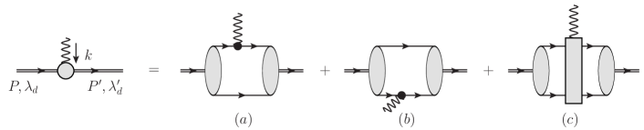
Figure 2: The matrix element $\Braket{P^{\prime},\lambda_{d}^{\prime}}{J^{\mu}}{P,\lambda_{d}}$ written as a sum of single-nucleon contributions (a) and (b) and the two-nucleon contribution (c). Single, double and wiggly lines refer to nucleons, deuteron particles and photons, respectively. Black dots and the gray rectangle denote the full photon-nucleon interaction vertex and the two-nucleon current operator.

In the Breit frame, the deuteron form factors are expressed in terms of the matrix elements of the electromagnetic current convolved with the deuteron wave functions, $\Braket{P^{\prime},\lambda_{d}^{\prime}}{J^{\mu}}{P,\lambda_{d}}$, according to Eqs. (16)-(18). The matrix elements read

$$\frac{1}{2P_{0}}\Braket{P^{\prime},\lambda_{d}^{\prime}}{J_{B}^{\mu}}{P,\lambda_{d}}=\!\!\int\frac{d^{3}l_{1}}{{(2\pi)}^{3}}\frac{d^{3}l_{2}}{{(2\pi)}^{3}}\,\psi^{\dagger}_{\lambda_{d}^{\prime}}\left(\bm{l}_{2}+\frac{\bm{k}}{4},\bm{v}_{B}\right)\,J^{\mu}_{B}\,\psi_{\lambda_{d}}\left(\bm{l}_{1}-\frac{\bm{k}}{4},-\bm{v}_{B}\right),$$ (19)

where $J^{\mu}_{B}$ is the four-vector current calculated in the Breit frame, $\psi_{\lambda}$ is the deuteron wave function with the polarization $\lambda$ and the deuteron in the final (initial) state moves with the velocity $\bm{v}_{B}$ ($-\bm{v}_{B}$) with $\bm{v}_{B}=\bm{k}/(2\sqrt{\bm{k}^{2}/4+m_{d}^{2}})=\hat{\bm{k}}\sqrt{\eta/(1+\eta)}$ and the momenta are defined in Eq. (11). This matrix element is visualized in Fig. 2, where diagrams (a) and (b) involve the single-nucleon electromagnetic current while diagram (c) corresponds to the matrix element of the two-nucleon current.

In this paper, we calculate the deuteron FFs in the framework of chiral EFT utilizing an expansion around the non-relativistic limit and taking into account relativistic corrections as required by power counting. Specifically, we start with the expressions for the single- and two-nucleon charge density operators, whose chiral expansion will be summarized in the next section. Using the deuteron wave functions at the corresponding order in the chiral expansion and employing consistently regularized expressions for the charge density operators in the partial wave basis, we calculate numerically the corresponding convolution integrals.

III Chiral expansion of the charge density operator

The nuclear electromagnetic charge and current operators have been recently worked out to N³LO in chiral EFT by our group using the method of unitary transformation  Kolling:2009iq ; Kolling:2011mt ; Krebs:2019aka and by the JLab-Pisa group employing time-ordered perturbation theory  Pastore:2008ui ; Pastore:2009is ; Pastore:2011ip , see also Ref. Park:1995pn for a pioneering study along this line. Following our works on the derivation of the electromagnetic currents  Kolling:2009iq ; Kolling:2011mt ; Krebs:2019aka and nuclear forces  Epelbaum:2014sza ; Reinert:2017usi ; Epelbaum:2014efa ; Bernard:2007sp ; Bernard:2011zr ; Krebs:2012yv ; Krebs:2013kha ; Epelbaum:2014sea , in this study we employ the Weinberg power counting for the operators constructed in chiral EFT. The hierarchy of the operators is based on the expansion parameter $q\in\{p/\Lambda_{b},\;M_{\pi}/\Lambda_{b}\}$ with $p$ being a typical soft scale and $\Lambda_{b}^{2}\sim m_{N}M_{\pi}$ (with $M_{\pi}$ for the pion mass) referring to the breakdown scale of the chiral expansion. This implies that the contributions to the charge and current operators appear at orders $q^{-3}$ (LO), $q^{-1}$ (NLO), $q^{0}$ (N²LO), $q^{1}$ (N³LO) and $q^{2}$ (N⁴LO). Notice that the JLab-Pisa group employed the counting scheme with $m_{N}\sim\Lambda_{b}$ used in the single-nucleon sector, so that their NLO corrections appear already at order $q^{-2}$. We further emphasize that the expressions for the two-nucleon charge and current densities in Refs. Kolling:2009iq ; Kolling:2011mt ; Krebs:2019aka and  Pastore:2008ui ; Pastore:2009is ; Pastore:2011ip do not completely agree with each other. The differences are, however, irrelevant for the calculation of the deuteron charge and quadrupole form factors. For a comprehensive review of the electroweak currents and a detailed comparison between the two sets of calculations see Ref. Krebs:2020pii .

III.1 Single-nucleon contributions to the charge density operator

At the chiral order we are working, the single-nucleon contributions to the charge density operator in the kinematics $N(p)+\gamma(k)\to N(p^{\prime})$ take a well-known form (see Refs. Friar:1997js ; Krebs:2019aka and references therein)

$$\rho_{\text{1N}}=e\left(1-\frac{{\bm{k}}^{2}}{8m_{N}^{2}}\right)G_{\text{E}}({\bm{k}}^{2})+ie\frac{2G_{\text{M}}({\bm{k}}^{2})-G_{\text{E}}({\bm{k}}^{2})}{4m_{N}^{2}}(\bm{\sigma}\cdot\bm{k}\times\bm{p}).$$ (20)

Here, $G_{\text{E}}({\bm{k}}^{2})$ and $G_{\text{M}}({\bm{k}}^{2})$ are the electric and magnetic form factors of the nucleon respectively, and $e$ is the absolute value of the electron charge. The single-nucleon form factors can be written in terms of the isospin projectors and the corresponding form factors of the proton and neutron

$$G_{\text{E}}({\bm{k}}^{2})=G_{\text{E}}^{p}({\bm{k}}^{2})\frac{1+\tau_{3}}{2}+G_{\text{E}}^{n}({\bm{k}}^{2})\frac{1-\tau_{3}}{2},$$

$$G_{\text{M}}({\bm{k}}^{2})=G_{\text{M}}^{p}({\bm{k}}^{2})\frac{1+\tau_{3}}{2}+G_{\text{M}}^{n}({\bm{k}}^{2})\frac{1-\tau_{3}}{2}.$$ (21)

For convenience, we also introduce the isoscalar nucleon form factors which are relevant for electron-deuteron scattering

$$G_{\text{E}}^{S}({\bm{k}}^{2}):=G_{\text{E}}^{p}({\bm{k}}^{2})+G_{\text{E}}^{n}({\bm{k}}^{2}),\qquad G_{\text{M}}^{S}({\bm{k}}^{2}):=G_{\text{M}}^{p}({\bm{k}}^{2})+G_{\text{M}}^{n}({\bm{k}}^{2}).$$ (22)

In order to facilitate the comparison with phenomenological studies, it is also convenient to decompose the single nucleon charge density from Eq. (20) into

$$\rho_{\text{1N}}=\rho^{\rm Main}_{\text{1N}}+\rho_{\text{1N}}^{\text{DF}}+\rho_{\text{1N}}^{\text{SO}},$$ (23)

with

$$\rho_{\text{1N}}^{\text{Main}}=eG_{\text{E}}({\bm{k}}^{2}),\hskip 28.45274pt\rho_{\text{1N}}^{\text{DF}}=e\left(-\frac{{\bm{k}}^{2}}{8m_{N}^{2}}\right)G_{\text{E}}({\bm{k}}^{2}),\hskip 28.45274pt\rho_{\text{1N}}^{\text{SO}}=ie\frac{2G_{\text{M}}({\bm{k}}^{2})-G_{\text{E}}({\bm{k}}^{2})}{4m_{N}^{2}}\bm{\sigma}\cdot\bm{k}\times\bm{p},$$ (24)

where, apart from the main contribution, DF and SO stand for the Darwin-Foldy and spin-orbit contributions, respectively. Terms involving order-$\mathcal{O}(m_{N}^{-4})$ corrections to the charge density are beyond the accuracy of our study.

The chiral expansion of the electromagnetic FFs of the nucleon is well known to converge slowly as they turn out to be dominated by contributions of vector mesons Kubis:2000zd ; Schindler:2005ke , which are not included as explicit degrees of freedom in chiral EFT. To minimize the impact of the slow convergence of the EFT expansion of the nucleon FFs on two-nucleon observables, the following two approaches can be employed:

• Instead of looking at the individual FFs of the deuteron $G_{\text{C}}$ and $G_{\text{Q}}$, one calculates the ratio $G_{\text{C}}/G_{\text{Q}}$ as done e.g. in Refs. Phillips:2003jz ; Phillips:2006im . This is advantageous if one can neglect the contribution of the magnetic form factor $G_{\text{M}}({\bm{k}}^{2})$ in Eq. (20). However, in addition to this, one also needs to assume either that the contributions from two-nucleon charge densities can be neglected altogether or that they scale with $G_{\text{E}}({\bm{k}}^{2})$ in the same way as the one-body densities. Then, the quantity $G_{\text{E}}({\bm{k}}^{2})$ drops out in the ratio $G_{\text{C}}/G_{\text{Q}}$. In this study, we show that two-nucleon charge density operators should indeed be proportional to $G_{\text{E}}({\bm{k}}^{2})$, see Sec. III.3 for details. We also note that due to the numerical smallness of the SO contribution, which is the only term proportional to $G_{\text{M}}({\bm{k}}^{2})$, considering this ratio may, in practice, indeed provide quite accurate results. On the other hand, formally, this approximation is not valid at the accuracy level of our analysis.

• Instead of relying on the strict chiral expansion of the nucleon FFs one can employ empirical parametrizations extracted from experimental data, as done e.g. in Ref. Valderrama:2007ja .

In this work, we utilize the second approach and use up-to-date parametrizations extracted from experimental data as will be described in the next section. The uncertainty of our results associated with the single-nucleon FFs will be addressed in Section VII.5.2.

III.2 Input for nucleon form factors

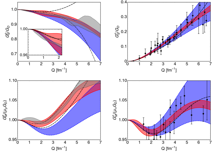
Figure 3: (Color online) The proton (left panel) and neutron (right panel) form factors normalized to the dipole form factor $G_{\text{D}}(Q^{2})={(1+Q^{2}/\Lambda_{D}^{2})}^{-2}$ with $\Lambda_{D}^{2}=0.71\text{ GeV}^{2}$. The gray bands between the dotted lines correspond to the proton form factors extracted in Ref. Bernauer:2013tpr from a combined fit to all data including polarized ratio measurements. The uncertainty corresponds to the combined statistical and systematic uncertainties taken in quadrature, among which the sensitivity to the functional form of the spline used in the fits is the largest. The red bands between the solid lines represent the results of the global analysis of the world proton observables and the neutron FFs from Ref. Ye:smallrp , see also Ref. Ye:2017gyb for the published version and text for the details. The blue bands between the dashed lines show the results of the SC approach of Ref. Belushkin:2006qa from a simultaneous dispersive analysis of all four FFs (data are also shown as dots — see Refs. Punjabi:2015bba ; Ye:2017gyb ; Belushkin:2006qa for more details) in both the space-like and time-like regions. The dashed lines show an update of the analysis of Ref. Belushkin:2006qa which is based on the fit to the MAMI data for electron-proton scattering and simultaneously to the world data for the neutron form factors Lorenz:2012tm . The dot-dashed lines represent the results for the proton FFs extracted using the dispersive approach of Ref. Lorenz:2014yda from a global analysis of the world data for electron-proton scattering. No errors for the nucleon FFs were given in Refs. Lorenz:2012tm and Lorenz:2014yda .

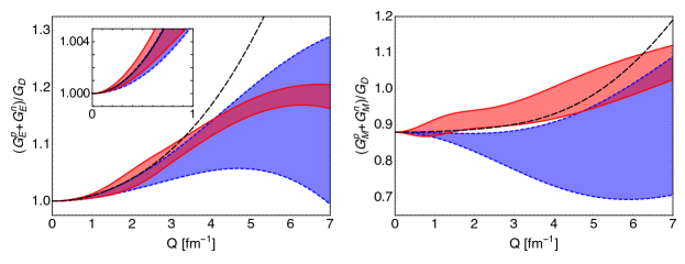
Figure 4: (Color online) Isoscalar nucleon electric (left panel) and magnetic (right panel) form factors normalized to the dipole form factor $G_{\text{D}}(Q^{2})$. For remaining notation see Fig. 3.

The electromagnetic form factors of the proton and neutron probe the charge and magnetization distributions of the nucleons via the interaction of electromagnetic currents and have been investigated experimentally for more than 70 years using electron scattering — see e.g. Refs. Punjabi:2015bba ; Pacetti:2015iqa ; Drechsel:2007sq ; Perdrisat:2006hj ; Arrington:2006zm for selected review articles.

The most recent extraction of the proton form factors was carried out in Refs. Ye:2017gyb ; Ye:smallrp , where a global analysis of all existing data was done including the corrections for different normalization of various data, and effects from TPE. The results of Ref. Ye:smallrp are shown in Fig. 3 (left panel) by red bands confined by solid lines. These fits were constrained at low $Q^{2}$ by the latest CODATA-2018 values for the proton charge radii CODATA2018 and by the magnetic radii from the Particle Data Group (PDG) Tanabashi:2018oca while at high $Q^{2}$ a power-law falloff was enforced. Another global analysis of the proton data was carried out by the A1 collaboration in Refs. Bernauer:2010wm ; Bernauer:2013tpr , where specific functional form for the form factors was assumed to fit the world data and no constraints on the proton radii were imposed. Apart from some differences in $G_{\text{M}}^{p}$ at low $Q^{2}$ and very large differences in the estimated uncertainties, the extracted electric and magnetic form factors of the proton in Refs. Ye:2017gyb ; Ye:smallrp and Bernauer:2013tpr are essentially consistent with each other, cf. red and gray bands in Fig. 3.

A determination of the neutron form factors is much more complicated than for the proton, since there are no free-neutron targets and it is, therefore, necessary to analyze experimental data on nuclear targets like ²H or ³He. A reliable extraction of the neutron form factors from such data requires a detailed understanding of the nuclear corrections (involving nuclear wave functions, final state interaction, meson exchange currents etc.). The results of the most up-to-date parametrization of the neutron FFs carried out in Ref. Ye:smallrp are presented in Fig. 3 (see red bands between solid lines in the right panel).

Already in Refs. Hohler:1976ax ; Mergell:1995bf , it was pointed out that analyticity and unitarity put strong constraints on the nucleon FFs. Using the spectral-function-based dispersive approach, the nucleon FFs were obtained in Ref. Belushkin:2006qa from a simultaneous fit to the data for all four FFs in both space-like and time-like regions including the constraints from meson-nucleon scattering data, unitarity, and perturbative QCD. The results of this analysis for the so-called “superconvergence approach” (SC) are shown as blue bands confined by the dashed lines in Fig. 3. An update of the analysis of Ref. Belushkin:2006qa based on the fit to the most recent MAMI data for electron-proton scattering and simultaneously to the world data for the neutron form factors was made in Ref. Lorenz:2012tm and shown in Fig. 3 by black long-dashed lines. Another strategy was used in the latest dispersive analysis of Ref. Lorenz:2014yda . First, the world experimental data on electron proton scattering were corrected in Ref. Lorenz:2014yda for the TPE contributions, which were calculated including the nucleon and $\Delta(1232)$-resonance intermediate states. Then, the corrected data were fitted using the proton FFs evaluated in the dispersive approach. No updates of the neutron FFs were made. The comparison of the results of the dispersive approach with those from the analysis in Refs. Ye:smallrp ; Ye:2017gyb reveals that the electric and magnetic proton FFs from Ref. Lorenz:2014yda are compatible with the band from Ref. Ye:smallrp at small and intermediate $Q$, although they visibly deviate from each other at $Q$ larger than $4$ fm^-1 (cf. dot-dashed curve with the red band). A closer look at the small momentum range, which is particularly sensitive to the proton charge radius, shows a very good agreement between the results of these analyses, see the zoomed plot for $G_{\text{E}}^{p}$ in Fig. 3. This is not surprising given that the value for the proton charge radius predicted in Ref. Lorenz:2014yda is consistent with the latest CODATA-2018 update employed in Ref. Ye:smallrp as input, see also Ref. Hammer:2019uab for a mini-review on the status of the proton radius puzzle.

Last but not least, the lattice QCD simulations for the nucleon FFs are already approaching the accuracy compatible with the experimental precision. For example, in Ref. Alexandrou:2017ypw , the electromagnetic FFs of the nucleon are computed including both the connected and disconnected contributions for the pion masses basically at the physical point. The resulting isoscalar and isovector nucleon FFs were found to overshoot the experimental data by about one standard deviation which, as proposed in Ref. Alexandrou:2017ypw , could be due to small residual excited state contamination. Further simulations should help in resolving this issue.

In this work, we will employ a set of different parametrizations for the proton and neutron FFs as input to calculate the deuteron FFs and, in this way, to make a complementary nontrivial test of our understanding of the nucleon FFs. Indeed, since our current study is aimed at a high-accuracy systematic investigation of the nuclear effects up to N⁴LO in chiral EFT, the comparison of the calculated deuteron form factors with data should provide useful insights into the consistency of the single nucleon input with the elastic scattering data on the deuteron. Since the up-to-date dispersive results from Refs. Lorenz:2012tm ; Lorenz:2014yda are given without uncertainties, we will use the results of Ref. Ye:2017gyb ; Ye:smallrp as our central input, while the FFs from Ref. Belushkin:2006qa will be employed as a consistency check.

Finally, since the deuteron FFs involve only the isoscalar combinations of the nucleon FFs, see Eq. (22), we plot these combinations in Fig. 4. Notice further that the charge and quadrupole FFs of the deuteron are sensitive predominantly to the isoscalar electric FF of the nucleon, while the isoscalar magnetic FF contributes only through the numerically small spin-orbit correction. For the isoscalar electric form factor, the dispersive results of Refs. Belushkin:2006qa ; Lorenz:2012tm are essentially consistent with each other as well as with those from the analysis Ye:smallrp at least for $Q\lesssim 3.5$ fm^-1.

III.3 Two-nucleon contributions to the charge density operator

The charge density operator is dominated by the LO single-nucleon contribution, while the first two-nucleon (2N) terms appear only at N³LO Kolling:2009iq ; Kolling:2011mt . The dominant contributions to the 2N charge density operator stem from one-loop diagrams of the one-pion exchange (OPE), two-pion exchange and contact types, whose explicit expressions are parameter-free and can be found in Refs. Kolling:2009iq ; Kolling:2011mt . All these terms are of isovector type and, therefore, do not contribute to the deuteron form factors. In addition to the already-mentioned static (i.e. order-${(1/m_{N})}^{0}$) contributions, one also has to consider tree-level one-pion exchange diagrams with a single insertion of the kinetic energy or $1/m_{N}$-corrections to the leading pion-nucleon vertex. In the two-nucleon kinematics

$$N(p_{1})+N(p_{2})+\gamma(k)\to N(p_{1}^{\prime})+N(p_{2}^{\prime})$$ (25)

with auxiliary three-momenta defined as $\bm{q}_{1}=\bm{p}_{1}^{\,\prime}-\bm{p}_{1}$ and $\bm{q}_{2}=\bm{p}_{2}^{\,\prime}-\bm{p}_{2}$, the isoscalar one-pion exchange charge density can be written as Kolling:2011mt

$$\rho_{\text{2N}}^{1\pi} = (1-2\bar{\beta}_{9})\frac{eg_{A}^{2}}{16F_{\pi}^{2}m_{N}}(\bm{\tau}_{1}\cdot\bm{\tau}_{2})\frac{(\bm{\sigma}_{1}\cdot\bm{k})(\bm{\sigma}_{2}\cdot\bm{q}_{2})}{\bm{q}_{2}^{2}+M_{\pi}^{2}}$$ (26)

$$+(2\bar{\beta}_{8}-1)\frac{eg_{A}^{2}}{16F_{\pi}^{2}m_{N}}(\bm{\tau}_{1}\cdot\bm{\tau}_{2})\frac{(\bm{\sigma}_{1}\cdot\bm{q}_{2})(\bm{\sigma}_{2}\cdot\bm{q}_{2})(\bm{q}_{2}\cdot\bm{k})}{{(\bm{q}_{2}^{2}+M_{\pi}^{2})}^{2}}+(1\leftrightarrow 2),$$

where the dimensionless quantities $\bar{\beta}_{8}$ and $\bar{\beta}_{9}$ parametrize the unitary ambiguity of the long-range contributions to the nuclear forces and currents at N³LO. The explicit form of the corresponding unitary transformations is given in Eq. (4.23) of Ref. Kolling:2011mt . Further, $g_{A}$ is the axial-vector coupling constant of the nucleon, $F_{\pi}$ is the pion decay constant and $(1\leftrightarrow 2)$ stands for a contribution resulting from interchanging the nucleon labels. Notice that the OPE contribution has also been taken into account in phenomenological studies, where it represents a part of the so-called meson-exchange currents, see e.g. Friar:1979by .

It is important to emphasize that all terms of the OPE charge density in Eq. (26) are proportional to unobservable unitary-transformation-parameters $\bar{\beta}_{8}$ and $\bar{\beta}_{9}$. The same parameters also appear in the $1/m_{N}^{2}$- and $1/m_{N}$-contributions to the two- Epelbaum:2004fk and three-nucleon forces at N³LO Bernard:2011zr , see also Ref. Friar:1999sj for a related discussion. This unitary ambiguity reflects the fact that nuclear forces and currents are not directly measurable and, in general, scheme-dependent. In contrast, observable quantities such as e.g. the form factors must, of course, be independent of the choice of $\bar{\beta}_{8}$, $\bar{\beta}_{9}$ and other off-shell parameters. This can only be achieved by using off-shell consistent expressions for the nuclear forces and currents. In particular, to be consistent with the new semilocal momentum-space regularized NN potentials of Refs. Reinert:2020mcu ; Reinert:2017usi which we employ to calculate the deuteron wave function (DWF) for our analysis, the so-called minimal nonlocality choice with

$$\bar{\beta}_{8}=1/4,\quad\quad\bar{\beta}_{9}=-1/4$$ (27)

has to be made. Note that the employed calculational approach relies on a numerically exact solution of the 2N Schrödinger equation with a potential truncated at a given order. This way one unavoidably includes certain higher-order contributions to the scattering amplitude so that the calculated observables are only expected to be approximately independent of $\bar{\beta}_{8}$, $\bar{\beta}_{9}$. The residual dependence on these parameters should be of a higher order, which provides a useful tool to check consistency of the calculations. In Section VII.5.5, we will demonstrate that the deuteron FFs calculated with different sets of $\bar{\beta}_{8}$, $\bar{\beta}_{9}$ yield consistent results.

An important consequence of the unitary ambiguity associated with $\bar{\beta}_{8}$ and $\bar{\beta}_{9}$ is that one can use unitary transformations to reshuffle the contributions to observables between the charge density and DWF. One can even completely eliminate the isoscalar 2N charge density operator at N³LO. As will be shown below, this also holds true for the short-range corrections at N⁴LO. The expression in Eq. (26) is thus to be understood as the contribution induced by acting with the unitary operator specified in Eq. (4.23) of Ref. Kolling:2011mt on the isoscalar part of the leading single-nucleon charge density operator $\rho_{\text{1N}}^{\text{Main, LO}}=e$, where the electric nucleon FF at leading order (labeled by the superscript LO) was set to unity. Since we do not rely on the chiral expansion of the nucleon FFs in our analysis, it is more consistent and appropriate to define the isoscalar OPE contribution as the one induced by $\rho_{\text{1N}}^{\text{Main}}$ rather than $\rho_{\text{1N}}^{\text{Main, LO}}$, which generalizes the expression in Eq. (26) to

$$\rho_{\text{2N}}^{1\pi} = (1-2\bar{\beta}_{9})G_{\text{E}}^{S}(Q^{2})\frac{eg_{A}^{2}}{16F_{\pi}^{2}m_{N}}(\bm{\tau}_{1}\cdot\bm{\tau}_{2})\frac{(\bm{\sigma}_{1}\cdot\bm{k})(\bm{\sigma}_{2}\cdot\bm{q}_{2})}{\bm{q}_{2}^{2}+M_{\pi}^{2}}$$

$$+(2\bar{\beta}_{8}-1)G_{\text{E}}^{S}(Q^{2})\frac{eg_{A}^{2}}{16F_{\pi}^{2}m_{N}}(\bm{\tau}_{1}\cdot\bm{\tau}_{2})\frac{(\bm{\sigma}_{1}\cdot\bm{q}_{2})(\bm{\sigma}_{2}\cdot\bm{q}_{2})(\bm{q}_{2}\cdot\bm{k})}{{(\bm{q}_{2}^{2}+M_{\pi}^{2})}^{2}}+(1\leftrightarrow 2).$$

While this expression is equivalent to Eq. (26) up to terms of a higher order, using Eq. (III.3) ensures that our results for the deuteron FFs are independent of the parameters $\bar{\beta}_{8}$ and $\bar{\beta}_{9}$ to a very high degree, as will be explicitly demonstrated in Section VII.5.5.

Although the pionic contributions to the isoscalar charge density at N⁴LO have not been worked out yet, the complete expression for the contact operators at N⁴LO is derived and given in Appendix B. The expression for the antisymmetrized isoscalar contact operators at N⁴LO reads:

$$\rho_{\text{Cont}} = 2e\left(A+B+\frac{C}{3}\right)\frac{\bm{\sigma}_{1}\cdot\bm{\sigma}_{2}+3}{4}\frac{1-\bm{\tau}_{1}\cdot\bm{\tau}_{2}}{4}\bm{k}^{2}+2e\,C\frac{1-\bm{\tau}_{1}\cdot\bm{\tau}_{2}}{4}\left((\bm{k}\cdot\bm{\sigma}_{1})(\bm{k}\cdot\bm{\sigma}_{2})-\frac{1}{3}\bm{k}^{2}(\bm{\sigma}_{1}\cdot\bm{\sigma}_{2})\right)$$ (29)

$$+2e\,(A-3B-C)\frac{1-\bm{\sigma}_{1}\cdot\bm{\sigma}_{2}}{4}\left(\frac{\bm{\tau}_{1}\cdot\bm{\tau}_{2}+3}{4}\right)\,\bm{k}^{2},$$

where the first (second) line in Eq. (29) contributes to the isospin-0-to-isospin-0 (isospin-1-to-isospin-1) channel and $A$, $B$, and $C$ denote the corresponding LECs. These LECs contribute to the deuteron FFs in two linear combinations $A+B+C/3$ and $C$. The expression in Eq. (29) agrees with the isoscalar part of the result published in Ref. Phillips:2016mov , while the corresponding isovector terms are different, see Appendix B. Notice further that the contact operator relevant for the quadrupole moment of the deuteron (the term $\sim C$ in Eq. (29)) was first derived in Ref. Chen:1999tn .

As already pointed out above, the short-range operators Eq. (29) can, in principle, also be eliminated via a suitable unitary transformation at the cost of changing the off-shell behavior of the NN potential. The corresponding unitary transformation acting on two-nucleon states is given in Ref. Reinert:2017usi and can be written as

$$U=e^{A{T}_{1}+B{T}_{2}+C{T}_{3}},$$ (30)

where the anti-Hermitean generators read

$${T}_{1} = \big{(}\bm{p}_{1}^{\prime 2}+\bm{p}_{2}^{\prime 2}-\bm{p}_{1}^{2}-\bm{p}_{2}^{2}\big{)},$$

$${T}_{2} = \big{(}\bm{p}_{1}^{\prime 2}+\bm{p}_{2}^{\prime 2}-\bm{p}_{1}^{2}-\bm{p}_{2}^{2}\big{)}(\bm{\sigma}_{1}\cdot\bm{\sigma}_{2}),$$ (31)

$${T}_{3} = \bm{\sigma}_{1}\cdot(\bm{p}_{1}-\bm{p}_{2}+\bm{p}_{1}^{\prime}-\bm{p}_{2}^{\prime})\;\bm{\sigma}_{2}\cdot(\bm{p}_{1}^{\prime}-\bm{p}_{2}^{\prime}-\bm{p}_{1}+\bm{p}_{2})+\bm{\sigma}_{1}\cdot(\bm{p}_{1}^{\prime}-\bm{p}_{2}^{\prime}-\bm{p}_{1}+\bm{p}_{2})\;\bm{\sigma}_{2}\cdot(\bm{p}_{1}-\bm{p}_{2}+\bm{p}_{1}^{\prime}-\bm{p}_{2}^{\prime}).$$

Here, $\bm{p}_{i}$ ($\bm{p}_{i}^{\prime}$) denote the initial and final momenta of the nucleons. However, in Refs. Reinert:2017usi ; Reinert:2020mcu , the freedom to perform such unitary transformations has already been exploited to eliminate the redundant contact interactions contributing to the ¹S₀ and ³S₁ partial waves and the mixing angle $\epsilon_{1}$ at N³LO. Therefore, to be consistent with the choice of the off-shell behavior adopted in the NN potentials of Ref. Reinert:2020mcu , the short-range contributions to the charge density in Eq. (29) have to be taken into account explicitly. Here, we follow the same procedure as in the case of the OPE charge density and employ the short-range charge density operator induced by applying the unitary transformation in Eq. (30) to the charge density operator $\rho_{\text{1N}}^{\text{Main}}$ from Eq. (24):

$$\delta\hat{\rho}=\hat{U}^{\dagger}\hat{\rho}_{\text{1N}}^{\text{Main}}\,\hat{U}-\hat{\rho}_{\text{1N}}^{\text{Main}}\simeq\left[\hat{\rho}_{\text{1N}}^{\text{Main}},A\hat{T}_{1}+B\hat{T}_{2}+C\hat{T}_{3}\right],$$ (32)

where square brackets denote a commutator and $\hat{X}$ indicates that the quantity $X$ is to be regarded as an operator rather than a matrix element with respect to momenta of the nucleons. Evaluating the commutator in the given kinematics yields the generalization of Eq. (29) for the contact isoscalar charge density

$$\rho_{\text{Cont}} = 2eG_{\text{E}}^{S}(\bm{k}^{2})\bigg{[}\left(A+B+\frac{C}{3}\right)\frac{\bm{\sigma}_{1}\cdot\bm{\sigma}_{2}+3}{4}\frac{1-\bm{\tau}_{1}\cdot\bm{\tau}_{2}}{4}\bm{k}^{2}+C\frac{1-\bm{\tau}_{1}\cdot\bm{\tau}_{2}}{4}\left((\bm{k}\cdot\bm{\sigma}_{1})(\bm{k}\cdot\bm{\sigma}_{2})-\frac{1}{3}\bm{k}^{2}(\bm{\sigma}_{1}\cdot\bm{\sigma}_{2})\right)$$ (33)

$$+(A-3B-C)\frac{1-\bm{\sigma}_{1}\cdot\bm{\sigma}_{2}}{4}\left(\frac{\bm{\tau}_{1}\cdot\bm{\tau}_{2}+3}{4}\right)\,\bm{k}^{2}\bigg{]},$$

where the nucleon FF $G_{\text{E}}^{S}({\bm{k}}^{2})$ coming from $\rho_{\text{1N}}^{\text{Main}}$ accounts for a non-pointlike nature of the NN$\gamma$ vertex. The linear combinations of the LECs $(A+B+C/3)$ and $C$ will be determined from the deuteron data as discussed in Section VI.3. The combination $(A-3B-C)$ corresponds to the isospin-$1$-to-isospin-$1$ transition and should be determined from other processes. For the complete expression including isovector terms the reader is referred to Appendix B.

Finally, we emphasize that the above expressions do not provide the complete contribution to the 2N charge density operator at N⁴LO. It is, however, conceivable that most (if not all) of the corrections of the one- and two-pion exchange range, which still have to be worked out, are of isovector type and, therefore, do not contribute to the deuteron FFs. We expect that isoscalar long-range contributions at N⁴LO not considered in our study are, to some extent, effectively taken into account by the short-range operators for not too high values of the momentum transfer. For the sake of brevity, we will refer to all results based on the short-range part of the 2N charge density operator in Eq. (33) as being N⁴LO.

IV Regularization of the charge density operator

We now discuss regularization of the charge-density operators introduced in the previous section. The single-nucleon charge density operator requires no regularization. However, two-nucleon contributions (both OPE and contact) have to be regularized, because of the divergent loop integrals appearing in the convolution with deuteron wave function. We specifically focus here on the consistency with the regularization of chiral NN potential Reinert:2020mcu ; Reinert:2017usi . The new generation of chiral NN potentials of Ref. Reinert:2020mcu ; Reinert:2017usi employed in our analysis make use of the local momentum-space regulator for pion exchange contributions, which, by construction, maintains the long-range structure of the nuclear force. The short-range part of the nuclear forces developed in Refs. Epelbaum:2014efa ; Epelbaum:2014sza is regularized with an angular-independent Gaussian momentum-space regulator. The meaning of consistency of the regularization procedure for nuclear forces and currents is discussed in Refs. Krebs:2019uvm ; Epelbaum:2019jbv , where it is shown that the usage of dimensionally regularized loop contributions to the three-nucleon forces and 2N currents leads, in general, to incorrect results for observables. In order to avoid this problem, loop contributions to the current operators need to be rederived using a regulator compatible with that employed in the NN potentials. The complications related to the loop operators are, however, irrelevant for our analysis: thanks to the deuteron acting as an isospin filter, none of the terms in the 2N charge density stemming from loop diagrams at N³LO contribute to the deuteron FFs. Still, it is important for our analysis to employ a proper regulator chosen in a way compatible with the NN potentials of Refs. Reinert:2020mcu ; Reinert:2017usi . In particular, since the contribution of the single-nucleon charge density to the deuteron FFs drops off rapidly with increasing values of the momentum transfer, the calculated FFs at larger $Q$-values become sensitive to the two-nucleon charge density operator which depends on the regulator.

We start with the OPE operators given by Eq. (III.3). These operators contain single and squared pion propagators. The regularization of the contributions with the single pion propagator is defined in Ref. Reinert:2017usi and can be effectively written as a substitution:

$$\frac{1}{\bm{p}^{2}+M_{\pi}^{2}}\to\frac{1}{\bm{p}^{2}+M_{\pi}^{2}}\exp\left(-\frac{\bm{p}^{2}+M_{\pi}^{2}}{\Lambda^{2}}\right),$$ (34)

where $\Lambda$ is a fixed cutoff chosen consistently with the employed NN potential in the range of $400$–$550$ MeV.

Apart from the single pion propagator, the OPE charge density, Eq. (III.3), also contains the pion propagator squared. The prescription for regularizing the squared pion propagator can be obtained from Eq. (34) by taking a derivative with respect to $M_{\pi}^{2}$, as done in Ref. Reinert:2017usi , which yields

$$\frac{1}{{(\bm{p}^{2}+M_{\pi}^{2})}^{2}}\to\left(\frac{1}{{(\bm{p}^{2}+M_{\pi}^{2})}^{2}}+\frac{1}{\Lambda^{2}(\bm{p}^{2}+M_{\pi}^{2})}\right)\exp\left(-\frac{\bm{p}^{2}+M_{\pi}^{2}}{\Lambda^{2}}\right).$$ (35)

Using the regularization procedure specified above, the regularized expression for the isoscalar part of the OPE charge density takes the form

$$\rho_{\text{2N}}^{1\pi,\,\text{reg}} = (1-2\bar{\beta}_{9})G_{\text{E}}^{S}(Q^{2})\frac{eg_{A}^{2}}{16F_{\pi}^{2}m_{N}}(\bm{\tau}_{1}\cdot\bm{\tau}_{2})\frac{(\bm{\sigma}_{1}\cdot\bm{k})(\bm{\sigma}_{2}\cdot\bm{q}_{2})}{\bm{q}_{2}^{2}+M_{\pi}^{2}}\exp\left(-\frac{\bm{q}_{2}^{2}+M_{\pi}^{2}}{\Lambda^{2}}\right)$$ (36)

$$+(2\bar{\beta}_{8}-1)G_{\text{E}}^{S}(Q^{2})\frac{eg_{A}^{2}}{16F_{\pi}^{2}m_{N}}(\bm{\tau}_{1}\cdot\bm{\tau}_{2})(\bm{\sigma}_{1}\cdot\bm{q}_{2})(\bm{\sigma}_{2}\cdot\bm{q}_{2})(\bm{q}_{2}\cdot\bm{k})$$

$$\times\left(\frac{1}{{(\bm{q}_{2}^{2}+M_{\pi}^{2})}^{2}}+\frac{1}{\Lambda^{2}(\bm{q}_{2}^{2}+M_{\pi}^{2})}\right)\exp\left(-\frac{\bm{q}_{2}^{2}+M_{\pi}^{2}}{\Lambda^{2}}\right)+(1\leftrightarrow 2).$$

As a next step, we consider the regularization of the contact charge density given by Eq. (33). To ensure consistency between regularizations of potential and charge density and avoid ambiguity due to the dependence of the charge density operator on the photon momentum, we exploit the fact that both the off-shell contact NN potential and the short-range charge density operators can be generated by the same unitary transformation acting on the kinetic energy term and the single-nucleon charge density, respectively. The contact part of the NN potential is regularized in Ref. Reinert:2017usi via a non-local Gaussian cutoff

$$V_{\text{Cont}}^{\text{reg}}=V_{\text{Cont}}\;\exp\left(-\frac{{(\bm{p}^{\prime}_{1}-\bm{p}^{\prime}_{2})}^{2}+{(\bm{p}_{1}-\bm{p}_{2})}^{2}}{4\Lambda^{2}}\right).$$ (37)

The regularized off-shell contact NN interactions can be obtained by applying the unitary transformation given by Eq. (30) to the kinetic energy term with the regularized generators $T_{i}$

$${T}_{i}^{\text{reg}}={T}_{i}\;\exp\left(-\frac{{(\bm{p}^{\prime}_{1}-\bm{p}^{\prime}_{2})}^{2}+{(\bm{p}_{1}-\bm{p}_{2})}^{2}}{4\Lambda^{2}}\right),\qquad i=1,2,3.$$ (38)

Then, by acting with this unitary transformation on the single-nucleon charge density $\rho_{\text{1N}}^{\text{Main}}$ from Eq. (24), we obtain the consistently regularized 2N short-range charge density operator:

$$\rho_{\text{Cont}}^{\text{reg}}=2eG_{\text{E}}^{S}({\bm{k}}^{2})\left((A+B\,(\bm{\sigma}_{1}\cdot\bm{\sigma}_{2}))F_{1}\left(\frac{\bm{p}_{1}-\bm{p}_{2}}{2},\frac{\bm{p}^{\prime}_{1}-\bm{p}^{\prime}_{2}}{2},\bm{k}\right)+CF_{2}\left(\frac{\bm{p}_{1}-\bm{p}_{2}}{2},\frac{\bm{p}^{\prime}_{1}-\bm{p}^{\prime}_{2}}{2},\bm{k}\right)\right),$$ (39)

where the functions $F_{1}$ and $F_{2}$ are defined as

$$F_{i}(\bm{p},\bm{p}^{\prime},\bm{k})=E_{i}\left(\bm{p}-\frac{\bm{k}}{2},\bm{p}^{\prime}\right)+E_{i}\left(\bm{p}+\frac{\bm{k}}{2},\bm{p}^{\prime}\right)+E_{i}\left(\bm{p}^{\prime}-\frac{\bm{k}}{2},\bm{p}\right)+E_{i}\left(\bm{p}^{\prime}+\frac{\bm{k}}{2},\bm{p}\right),$$ (40)

with

$$E_{1}\left(\bm{p},\bm{p}^{\prime}\right) = \left(\bm{p}^{2}-\bm{p}^{\prime 2}\right)\,\exp\left(-\frac{\bm{p}^{2}+\bm{p}^{\prime 2}}{\Lambda^{2}}\right),$$

$$E_{2}\left(\bm{p},\bm{p}^{\prime}\right) = \left[(\bm{\sigma}_{1}\cdot\bm{p})(\bm{\sigma}_{2}\cdot\bm{p})-(\bm{\sigma}_{1}\cdot\bm{p}^{\prime})(\bm{\sigma}_{2}\cdot\bm{p}^{\prime})\right]\,\exp\left(-\frac{\bm{p}^{2}+\bm{p}^{\prime 2}}{\Lambda^{2}}\right).$$ (41)

Note that, similarly to the procedure used for obtaining the contact interactions, the regularized OPE contribution to the 2N charge density (as given in Eq. (36)) can also be derived by regularizing the long-range unitary transformation (as given in Eq. (4.23) of Ref. Kolling:2011mt ) and acting with it on the single-nucleon charge density $\rho_{\text{1N}}^{\text{Main}}$ from Eq. (24).

Equations (36) and (39) provide the final expressions for the 2N charge density operator at N³LO and N⁴LO used in the calculation of the deuteron FFs.

V Relativistic corrections

Although the deuteron FFs are Lorentz-invariant, the individual ingredients (charge density operators and deuteron wave functions) do depend on the reference frame. At N²LO and below, all frame-dependent corrections are irrelevant, but starting from N³LO, the relativistic corrections to each ingredient have to be systematically taken into account. Frame dependence of the charge density operator is automatically accounted for by the kinematics, because the operator is calculated explicitly including all relevant $1/m_{N}$ corrections. In this section, we will focus on the relativistic corrections to the deuteron wave functions stemming from the motion of the initial and final deuterons.

The DWF is typically calculated for the deuteron at rest. However, a calculation of the deuteron FFs always involves at least one moving deuteron. Our calculation is carried out in the Breit frame, where the initial and final deuterons are moving in opposite directions. To account for this motion, the rest-frame DWF needs to be boosted. To the chiral order we are working (N⁴LO), the DWF boost corrections have to be considered only when calculating the convolution integrals of the DWF with the leading single-nucleon charge density $\rho_{\text{1N}}^{\text{Main}}$ from Eq. (24).

Since subleading corrections to the single-nucleon charge density as well as the first contributions to the two-nucleon charge density appear only at N³LO, see Sections III and VI.3, the corresponding DWF-boost corrections are beyond the scope of our study.

Different approaches have been considered in the literature to include the DWF boost corrections and found to yield basically the same results. In Ref. Arnold:1979cg , a covariant relativistic calculation of the deuteron form factor was performed, and the final result was expanded in powers of $1/m_{N}$, see also Ref. Gilman:2001yh for a review. Alternatively, boosted DWF was calculated in Refs. Krajcik:1974nv ; Friar:1977xh ; Ritz:1996za ; Wallace:2001nv ; Schiavilla:2002fq utilizing the $1/m_{N}$ expansion of the generators of the Poincaré group. This is the approach we follow in our analysis. For a deuteron moving with the velocity $\bm{v}$, the boosted DWF operator has the form Schiavilla:2002fq

$$\psi(\bm{p},\bm{v})\simeq\left(1-\frac{\bm{v}^{2}}{4}\right)\left[1-\frac{1}{2}(\bm{v}\cdot\bm{p})(\bm{v}\cdot\bm{\nabla}_{\!p})-\frac{i}{4m_{N}}\bm{v}\cdot(\bm{\sigma}_{1}-\bm{\sigma}_{2})\times\bm{p}\right]\psi(\bm{p},0),$$ (42)

where $\bm{p}$ is the relative momentum of two nucleons, and $\psi(\bm{p},0)$ is the rest-frame DWF which is normalized as

$$\int\frac{d^{3}p}{(2\pi)^{3}}\,|\psi\left(\bm{p},0\right)|^{2}=\int\frac{d^{3}p}{(2\pi)^{3}}\,|\psi\left(\bm{p},\bm{v}\right)|^{2}=1\,.$$ (43)

Then, to the order we are working, the boost-corrected matrix element (19) evaluated with the leading density $\rho_{\text{1N}}^{\text{Main}}$ reads

$$\frac{1}{2P_{0}}\Braket{P^{\prime},\lambda_{d}^{\prime}}{\rho_{\text{1N}}^{\text{Main}}}{P,\lambda_{d}} = e\,G_{\text{E}}^{S}({\bm{k}}^{2})\int\frac{d^{3}p}{{(2\pi)}^{3}}\,\psi_{\lambda_{d}^{\prime}}^{\dagger}\left(\bm{p}+\frac{\bm{k}_{\text{boosted}}}{4},0\right)\,\psi_{\lambda_{d}}\left(\bm{p}-\frac{\bm{k}_{\text{boosted}}}{4},0\right),$$ (44)

where

$$\bm{k}_{\text{boosted}}=\bm{k}\sqrt{1-v_{B}^{2}}=\frac{\bm{k}}{\sqrt{1+\eta}},$$ (45)

and we used the fact that the spin dependent term in Eq. (42) vanishes for spin-$1$-to-spin-$1$ transitions relevant for the deuteron FFs.

The term on the rhs of Eq. (44) is related to the length contraction of that part of the relative nucleon momentum in the deuteron which is parallel to $\bm{k}$. As a consequence of this contraction, the matrix element must be evaluated with the deuteron wave function taken in its rest frame but with the Breit momentum $\bm{k}$ replaced by $\bm{k}_{\text{boosted}}$.

Finally, we remind the reader on the ambiguity of the relativistic corrections to the NN potential associated with the employed form of the Schrödinger equation. The corrections to the kinetic energy of relative motion of the nucleons are most easily taken into account by replacing the nonrelativistic expression $\bm{p}^{2}/m_{N}$ with $2\sqrt{\bm{p}^{2}+m_{N}^{2}}-2m_{N}$ instead of using the Taylor expansion, since otherwise the spectrum of the 2N Hamiltonian is unbounded from below. Instead of solving the corresponding relativistic Schrödinger equation, it is more convenient to rewrite it in the equivalent nonrelativistic form as explained in Ref. Friar:1999sj . This choice was adopted in the Nijmegen partial wave analysis Stoks:1993tb and is made in the chiral NN potentials of Refs. Epelbaum:2014efa ; Epelbaum:2014sza ; Reinert:2017usi ; Reinert:2020mcu . While rewriting the Schrödinger equation does affect the $m_{N}^{-1}$ and $m_{N}^{-2}$ contributions to the NN potential, the deuteron wave function remains unchanged so that we can directly employ the DWF from Refs. Reinert:2017usi ; Reinert:2020mcu .

VI Anatomy of the calculation

In this section, we summarize the analytic expressions for the deuteron charge and quadrupole form factors, as well as for the charge radius and the quadrupole moment. We discuss the individual contributions to these quantities from different types of the charge density introduced in the previous sections. We define the structure radius of the deuteron and argue, following Ref. Filin:2019eoe , that a high-accuracy calculation of this quantity along with high-precision atomic data for the 1S-2S hydrogen-deuterium isotope shift provide access to the neutron charge radius.

VI.1 The charge form factor and structure radius of the deuteron

The deuteron charge form factor $G_{\text{C}}$ can, up to N⁴LO, be written as

$$G_{\text{C}}(Q^{2})=G_{\text{C}}^{\text{Main}}(Q^{2})+G_{\text{C}}^{\text{DF}}(Q^{2})+G_{\text{C}}^{\text{SO}}(Q^{2})+G_{\text{C}}^{\text{Boost}}(Q^{2})+G_{\text{C}}^{1\pi}(Q^{2})+G_{\text{C}}^{\text{Cont}}(Q^{2}),$$ (46)

where $G_{\text{C}}^{\text{Main}}(Q^{2})$, $G_{\text{C}}^{\text{DF}}(Q^{2})$, and $G_{\text{C}}^{\text{SO}}(Q^{2})$ arise from charge densities defined in Eq. (24), $G_{\text{C}}^{\text{Boost}}(Q^{2})$ is a relativistic correction due to initial and final deuteron motion, $G_{\text{C}}^{1\pi}(Q^{2})$ stems from the one-pion-exchange charge density in Eq. (36), and $G_{\text{C}}^{\text{Cont}}(Q^{2})$ is generated by the contact charge density in Eq. (39). The main contribution $G_{\text{C}}^{\text{Main}}(Q^{2})$ can be factorized as

$$G_{\text{C}}^{\text{Main}}(Q^{2})=(G_{\text{E}}^{p}(Q^{2})+G_{\text{E}}^{n}(Q^{2}))G_{\text{C}}^{\text{matter}}(Q^{2}),$$ (47)

where $G_{\text{E}}^{p}(Q^{2})$ and $G_{\text{E}}^{n}(Q^{2})$ are the electric FFs of the proton and neutron, while $G_{\text{C}}^{\text{matter}}(Q^{2})$ is a functional of the deuteron wave function.

Charge conservation restricts the behavior of the charge form factor at $Q^{2}=0$. In particular, $G_{\text{C}}(0)=G_{\text{C}}^{\text{Main}}(0)=G_{\text{C}}^{\text{matter}}(0)=G_{\text{E}}^{p}(0)=1$, while all other contributions to $G_{\text{C}}$ vanish at $Q^{2}=0$.

The deuteron charge radius can be expressed as a derivative of the charge form factor with respect to $Q^{2}$ at $Q^{2}=0$

$$r_{d}^{2}=-6{\left.\frac{\partial G_{\text{C}}(Q^{2})}{\partial Q^{2}}\right|}_{Q^{2}=0}.$$ (48)

Taking derivatives of all terms in Eq. (46), we get the complete set of contributions to the deuteron charge radius up to N⁴LO

$$r_{d}^{2}=r_{m}^{2}+r_{p}^{2}+r_{n}^{2}+r_{\rm DF}^{2}+r_{\rm SO}^{2}+r_{\rm Boost}^{2}+r_{1\pi}^{2}+r_{\rm Cont}^{2},$$ (49)

where the deuteron matter radius $r_{m}$, the proton charge radius $r_{p}$ and the neutron charge radius $r_{n}$ are defined as:

$$r_{m}^{2}=-6{\left.\frac{\partial G_{\text{C}}^{\text{matter}}(Q^{2})}{\partial Q^{2}}\right|}_{Q^{2}=0},\qquad r_{p}^{2}=-6{\left.\frac{\partial G_{\text{E}}^{p}(Q^{2})}{\partial Q^{2}}\right|}_{Q^{2}=0},\qquad r_{n}^{2}=-6{\left.\frac{\partial G_{\text{E}}^{n}(Q^{2})}{\partial Q^{2}}\right|}_{Q^{2}=0},$$ (50)

and the remaining corrections to the deuteron charge radius are calculated as

$$r_{i}^{2}=-6{\left.\frac{\partial G_{\text{C}}^{i}(Q^{2})}{\partial Q^{2}}\right|}_{Q^{2}=0},\qquad i=\{\text{DF},\,\text{SO},\,\text{Boost},\,{1\pi},\,\text{Cont}\}.$$ (51)

Since the $r_{\text{DF}}$-term and the charge radii of the individual nucleons are not related to the two-body dynamics of the deuteron, they can be conveniently subtracted from the deuteron charge radius. The resulting quantity is referred to as the deuteron structure radius and is defined as (see, e.g. Ref Jentschura:2011NOTinHep )

$$r_{\rm str}^{2}=r_{d}^{2}-(r_{p}^{2}+r_{n}^{2}+r_{\rm DF}^{2}).$$ (52)

The deuteron-proton mean-square charge radii difference $r_{d}^{2}-r_{p}^{2}$ in Eq. (52) can be extracted experimentally with an extremely high precision from spectroscopic measurements of the 1S-2S hydrogen-deuterium isotope shift Jentschura:2011NOTinHep . In particular, a series of very precise measurements of the 1S-2S isotope shift, accompanied with an accurate theoretical QED analysis (see Ref. Pachucki:2018yxe for the latest update up through $O(\alpha^{2})$), resulted in the extraction of the deuteron-proton mean-square charge radii difference Jentschura:2011NOTinHep

$$r_{d}^{2}-r_{p}^{2}=3.82007(65)\text{fm}^{2}.$$ (53)

Due to its high accuracy, this difference provides a tight link between $r_{d}$ and $r_{p}$ and thus is important in connection with the light nuclear charge radius puzzle. For many years, the values for $r_{p}$ extracted from electron and muon experiments showed more than a 5$\sigma$ discrepancy Pohl:2013yb . The very recent atomic hydrogen measurements Beyer:2017gug ; Bezginov:2019mdi , however, claim consistency with the analogous muonic hydrogen experiments. The recommended value for the proton root-mean-square charge radius has been changed to $r_{p}=0.8414(19)$ fm in the latest CODATA-2018 update CODATA2018 , and the deuteron charge radius was updated accordingly, by virtue of the difference in Eq. (53). The updated CODATA deuteron charge radius is only 1.9$\sigma$ larger than the spectroscopic measurement on the muonic deuterium Pohl1:2016xoo but still 2.9$\sigma$ smaller than the $r_{d}$ value from electronic deuterium spectroscopy Pohl:2016glp .

As follows from Eq. (52), the deuteron-proton charge radii difference from Eq. (53) allows one to extract the difference $r_{\rm str}^{2}-r_{n}^{2}$ to a very high accuracy. The neutron charge radius can be deduced from measurements of the coherent neutron-electron scattering length extracted from data on neutron scattering off ²⁰⁸Pb, ²⁰⁹Bi and other heavy atoms. The value for the neutron charge radius quoted by the PDG is $r_{n}^{2}=-0.1161(22)\text{fm}^{2}$, where the estimated error was increased by a scaling factor of $1.3$ Tanabashi:2018oca . This value is based on averaging the results of four different experiments from years 1973 to 1997. In Ref. Jentschura:2011NOTinHep , the value of $r_{n}^{2}=-0.114(3)\text{fm}^{2}$, which is consistent with the PDG result, was employed based on the measurement on ²⁰⁸Pb from Ref. Kopecky:1997rw . Using this neutron radius and Eq. (53) for the deuteron-proton charge radii difference, the value of $r_{\text{str}}=1.97507(78)\text{ fm}$ for the structure radius was extracted Jentschura:2011NOTinHep . On the other hand, as advocated in Ref. Mitsyna:2009zz , the uncertainty for the neutron radius given above might suffer from the underestimation of systematic errors. For example, the central values on ²⁰⁸Pb and ²⁰⁹Bi quoted in the most recent investigation of Ref. Kopecky:1997rw differ from each other by 0.0090 $\text{fm}^{2}$, which is much larger than even the increased uncertainty given by the PDG. Therefore, a different logical chain was adopted in Ref. Filin:2019eoe , namely, (a) by employing the nuclear forces and currents derived up through fifth order in chiral EFT, a very accurate determination of $r_{\text{str}}$ is becoming possible based on the analysis of the deuteron charge form factor; (b) by using the predicted value for the deuteron structure radius together with the atomic data for the deuteron-proton charge radii difference, the charge radius of the neutron was for the first time extracted from light nuclei. In this investigation, we follow the same logic to update the analysis of Ref. Filin:2019eoe . In particular, we employ the updated NN potentials which include isospin breaking corrections up through N⁴LO and provide a statistically perfect description of neutron-proton and proton-proton scattering data up to the pion production threshold Reinert:2020mcu to extract the structure radius from a combined analysis of the charge and quadrupole deuteron FFs in the range of momentum transfer up to $Q=6$ fm^-1. Then, we update the value for the neutron charge radius, see Sec.VII.3 for the results.

VI.2 The quadrupole form factor and quadrupole moment of the deuteron

Deuteron quadrupole form factor can be decomposed in the same way as the charge form factor, namely:

$$G_{\text{Q}}(Q^{2})=G_{\text{Q}}^{\text{Main}}(Q^{2})+G_{\text{Q}}^{\text{DF}}(Q^{2})+G_{\text{Q}}^{\text{SO}}(Q^{2})+G_{\text{Q}}^{\text{Boost}}(Q^{2})+G_{\text{Q}}^{1\pi}(Q^{2})+G_{\text{Q}}^{\text{Cont}}(Q^{2}),$$ (54)

where the individual terms originate from different charge-density contributions in full analogy with Eq. (46). The deuteron quadrupole moment is defined as the value of the quadrupole form factor at $Q^{2}=0$, namely

$$Q_{d}=\frac{1}{m_{d}^{2}}G_{\text{Q}}(0).$$ (55)

Taking the $Q^{2}=0$ limit in Eq. (54) yields the individual contributions to the deuteron quadrupole moment, which read

$$Q_{d}=Q_{0}+Q_{\rm SO}+Q_{\rm Boost}+Q_{1\pi}+Q_{\rm Cont},$$ (56)

where we used the fact that $G_{\text{Q}}^{\text{DF}}(0)=0$ and defined the individual terms as

$$Q_{0} = \frac{1}{m_{d}^{2}}G_{\text{Q}}^{\text{Main}}(0),\qquad Q_{i}=\frac{1}{m_{d}^{2}}G_{\text{Q}}^{i}(0),\qquad i=\{\text{SO},\,\text{Boost},\,{1\pi},\,\text{Cont}\}.$$ (57)

The analytic expressions for various contributions to the deuteron charge and quadrupole form factors as well as to the structure radius and the quadrupole moment are collected in Appendix A.

VI.3 Calculational setup

The deuteron FFs at different chiral orders are calculated as follows:

• LO:
  The main contribution to the single-nucleon charge density $\rho_{\text{1N}}^{\text{Main}}$ in Eq. (24) is convoluted with the LO deuteron wave function.

• NLO:
  Same as LO but using the NLO deuteron wave function.

• N²LO:
  Same as LO but using the N²LO deuteron wave function.

• N³LO:
  The contributions $\rho_{\text{1N}}^{\text{Main}}$, $\rho_{\text{1N}}^{\text{DF}}$ and $\rho_{\text{1N}}^{\text{SO}}$ from Eq. (24) to the single-nucleon charge density and the OPE contribution in Eq. (36) are convoluted with the N³LO deuteron wave functions; the relativistic boost corrections to the single-nucleon contributions are calculated as explained in Section V.

• N⁴LO:
  Same as N³LO but using the N⁴LO⁺ deuteron wave function and including the 2N short-range charge density operators from Eq. (39).

Unless specified otherwise, all results presented below are based on the semilocal momentum-space NN potentials of Ref. Reinert:2017usi , updated to incorporate a more complete treatment of isospin-breaking corrections Reinert:2020mcu . In particular, the updated potentials take into account the charge dependence of the pion-nucleon coupling constants. The determination of the pion-nucleon coupling constants from NN data in Ref. Reinert:2020mcu leads to the average value of $g_{\pi N}$, which is about $1\%$ larger than the one employed in Ref. Reinert:2017usi , and the resulting change in the deuteron wave function leads to a visible effect on the quadrupole FF of the deuteron at higher $Q$-values. Clearly, in all cases, the same cutoff value chosen from the set $\Lambda=\{400,\,450,\,500,\,550\}$ MeV is used in the regularized NN potential and in the 2N charge density. For single-nucleon FFs, we employ the most up-to-date parametrization by Ye et al. Ye:smallrp for our central results. We propagate the uncertainty in the determination of these FFs to estimate its impact on the deuteron FFs in Section VII.5.2. In the same section we also consider the impact of using different single-nucleon FFs parametrizations.

It remains to specify the values of the various parameters used in the expressions for the 2N charge density operator in Eqs. (36) and (39). Following Refs. Reinert:2017usi ; Reinert:2020mcu , we employ the value of $g_{A}=1.29$ for the effective axial-vector coupling constant, which accounts for the Goldberger-Treiman discrepancy, $F_{\pi}=92.4$ MeV for the pion decay constant, $m_{N}=2m_{p}m_{n}/(m_{p}+m_{n})=938.918$ MeV for the nucleon mass and $M_{\pi}=(2{M_{\pi}}_{\pm}+{M_{\pi}}_{0})/3=138.03$ MeV for the pion mass. Notice that the expressions for the 2N charge density are taken in the isospin limit as the corresponding isospin-breaking corrections start to contribute at N⁵LO, which is beyond the accuracy of our analysis. Finally, the two linear combinations of LECs entering the short-range part of the 2N charge density operator at N⁴LO are determined from the best combined fit to the experimental data on the momentum-transfer dependence of the charge and quadrupole deuteron FFs as described in Section VII. This then allows us to make a parameter-free prediction for the structure radius and the quadrupole moment of the deuteron.

VII Results for charge and quadrupole deuteron form factors

In this section, we present our results for the deuteron charge and quadrupole form factors. We fix two LECs appearing in the N⁴LO contact charge density by fitting the calculated FFs, $G_{\text{C}}^{\text{th}}(Q)$ and $G_{\text{Q}}^{\text{th}}(Q)$, to the corresponding world experimental data for $Q<6$ fm^-1. Using the LECs extracted from the best fit, we predict the structure radius and the quadrupole moment of the deuteron. Following Ref. Filin:2019eoe , we use the predicted structure radius to extract the neutron charge radius from the precisely measured deuteron-proton charge-radii difference. We provide a detailed analysis of various uncertainties, discuss several important consistency checks, and discuss the role of the individual contributions to the charge and quadrupole deuteron form factors.

VII.1 Fitting procedure

The values of the LECs appearing in the N⁴LO contact charge density of Eq. (39) are determined from a $\chi^{2}$-fit of our theoretical predictions for $G_{\text{C}}^{\text{th}}(Q)$ and $G_{\text{Q}}^{\text{th}}(Q)$ to the experimental data. The analytic expressions for the individual contributions to $G_{\text{C}}^{\text{th}}(Q)$ and $G_{\text{Q}}^{\text{th}}(Q)$ are given in Appendix A, and the experimental data set used in the fit is described in Section II.4. In the infinite cutoff limit, $G_{\text{C}}^{\text{th}}(Q)$ depends only on one combination of the LECs, namely $A+B+C/3$, while $G_{\text{Q}}^{\text{th}}(Q)$ depends only on the LEC $C$. Once the regularization is applied, both $G_{\text{C}}^{\text{th}}(Q)$ and $G_{\text{Q}}^{\text{th}}(Q)$ in general depend on the two mentioned linear combinations of the LECs, see Eqs. (100) and (104) in Appendix A. The function $\chi^{2}(A+B+C/3;C)$ to be minimized is defined as follows

$$\chi^{2}=\sum_{i}\frac{{\bigl{(}G_{\text{C}}^{\text{th}}(Q^{2}_{i};A+B+C/3;C)-G_{\text{C}}^{\text{exp}}(Q^{2}_{i})\bigl{)}}^{2}}{\Delta G_{\text{C}}{(Q_{i}^{2})}^{2}}+\sum_{i}\frac{{\bigl{(}G_{\text{Q}}^{\text{th}}(Q^{2}_{i};A+B+C/3;C)-G_{\text{Q}}^{\text{exp}}(Q^{2}_{i})\bigl{)}}^{2}}{\Delta G_{\text{Q}}{(Q_{i}^{2})}^{2}},$$ (58)

where $\{Q_{i}\}$ are the set of momenta, for which experimental data are available, and the summations are performed for $Q_{i}$ below $Q_{\text{max}}=6$ fm^-1. The intrinsic systematic uncertainty related to the choice of $Q_{\text{max}}$ will be discussed below. Following Refs. Carlsson:2015vda ; Wesolowski:2018lzj , the uncertainties $\Delta G_{\text{C}}(Q_{i}^{2})$ and $\Delta G_{\text{Q}}(Q_{i}^{2})$ in $\chi^{2}$ include, apart from the experimental errors, also theoretical uncertainties added in quadrature

$$\Delta G_{\text{X}}{(Q_{i}^{2})}^{2} = \Delta G_{\text{X}}^{\text{exp}}{(Q_{i}^{2})}^{2}+\Delta G_{\text{X}}^{\text{th,trunc}}{(Q_{i}^{2})}^{2}+\Delta G_{\text{X}}^{\text{th,nuclFF}}{(Q_{i}^{2})}^{2},\qquad(X=\text{C and Q}).$$ (59)

In this way, we take into account uncertainties from the truncation of the chiral expansion and from the parametrization of the nucleon form factors. As the expansion parameter in chiral EFT increases with the momentum transfer, the truncation errors also grow with $Q$, as discussed in Section VII.5.1. Thus the inclusion of the truncation errors directly in the objective function allows us to use the deuteron data in a larger range of $Q$, namely up to $Q_{\text{max}}=6$ fm^-1 and even higher. The uncertainty related to the parametrization of the nucleon FFs is yet another source of the theoretical uncertainty which we include directly in the fit, see Section VII.5.2 for details. Other kinds of uncertainties such as the ones associated with the choice of $Q_{\text{max}}$ and with the $\pi$N and 2N LECs used in the NN potential are estimated separately and discussed below.

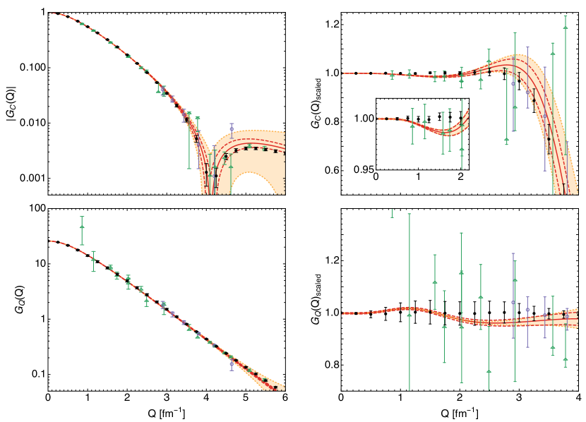
Figure 5: (Color online) Left panel: the deuteron charge and quadrupole FFs calculated at N⁴LO for the cutoff choice of $\Lambda=500$ MeV (solid red lines) along with the estimated truncation error ($68\%$ degree-of-belief) shown by the light-shaded band. Bands between dashed (red) lines correspond to a 1$\sigma$ error in the determination of the two short-range contributions at N⁴LO. Right panel: the same form factors divided by the scaling functions as defined in Eq. (63) and (64). Open violet circles and green triangles are experimental data from Refs. Nikolenko:2003zq and Abbott:2000ak , respectively. Black solid circles correspond to the parametrization of the deuteron FFs from Refs. Marcucci:2015rca ; Sick:priv .

Our central fit is performed for the cutoff $\Lambda=500$ MeV and $Q_{\text{max}}=6$ fm^-1. Assuming that the experimental data points are independent, the resulting $\chi^{2}$ and $\chi^{2}/\text{d.o.f.}$ values are

$$\chi^{2}_{\text{min}}=15.24,\qquad\chi^{2}_{\text{min}}/\text{d.o.f.}=0.34.$$ (60)

The low value of $\chi^{2}_{\text{min}}/\text{d.o.f.}$ may signal an overestimation of the truncation errors, but it can also be caused by neglecting correlations when estimating truncation errors at similar values of the momentum transfer. The value of $\chi^{2}_{\text{min}}/\text{d.o.f.}$, therefore, does not allow for a straightforward statistical interpretation. The obtained values of the two relevant linear combinations of the LECs read

$$A+B+\frac{C}{3} = (-281\pm 64)\text{ GeV}^{-5}\simeq(-0.66\pm 0.15)\frac{1}{F_{\pi}^{2}\Lambda_{b}^{3}},$$

$$C = (-58\pm 35)\text{ GeV}^{-5}\simeq(-0.14\pm 0.08)\frac{1}{F_{\pi}^{2}\Lambda_{b}^{3}},$$ (61)

where the error corresponds to the 1$\sigma$ deviation of the $\chi^{2}$ and $\Lambda_{b}=650\text{ MeV}$ refers to the breakdown scale of the chiral expansion, see Sec.VII.5.1 for a discussion. Notice that the both linear combinations of the LECs come out of a natural size, see the second equalities in Eq. (61). This is an important consistency check of our calculations, which is also fulfilled for the contact interactions entering the employed NN potentials, see Fig. 7 of Ref. Epelbaum:2019kcf . Finally, the correlation matrix for $A+B+C/3$ and $C$ reads

$$\rho=\begin{pmatrix}1&-0.4\\ -0.4&1\end{pmatrix}.$$ (62)

VII.2 Results for the deuteron form factors

The results for the deuteron charge and quadrupole FFs from the best fit to data up to $Q=6$ fm^-1, evaluated for the cutoff $\Lambda=500$ MeV, are visualized in Fig. 5 together with the N⁴LO truncation errors and statistical uncertainty of the LEC’s in $\rho_{\text{Cont}}^{\text{reg}}$ from Eq. (39). The plot contains two theoretical uncertainty bands: the light-shaded band stands for the estimated truncation error corresponding to the $68\%$ degree-of-belief interval, while the band between long-dashed (red) lines corresponds to a 1$\sigma$ error in the determination of the two short-range contributions at N⁴LO. In principle, these two uncertainty bands are not fully independent since the truncation error is also included in the estimate of the 1$\sigma$ error for the LECs in the charge density operator as discussed in previous Section. In this way, however, the truncation error is estimated more conservatively.

Since the variation of the FFs at small $Q$-values is difficult to see on the logarithmic scale, we also plot the rescaled FFs using a linear scale in the right panels of Fig. 5. Specifically, following Ref. Marcucci:2015rca , we define the rescaled charge and quadrupole FFs via

$$G_{\text{C}}^{\rm scaled}(Q)=G_{\text{C}}(Q){\left(\sum_{i=0}^{3}a_{i}\exp(-b_{i}Q^{2})\right)}^{-1}\,,$$ (63)

with $a_{1}=0.295$, $a_{2}=0.637$, $a_{3}=0.010$, $b_{0}=3.149$ fm², $b_{1}=1.183$ fm², $b_{2}=0.346$ fm², $b_{3}=0.036$ fm² and $a_{0}=1-a_{1}-a_{2}-a_{3}$ and

$$G_{\text{Q}}^{\rm scaled}(Q) = \frac{G_{\text{Q}}(Q)}{m_{d}^{2}\,Q_{d}}{\left(\sum_{i=0}^{3}a_{i}\exp(-b_{i}Q^{2})\right)}^{-1}\,,$$ (64)

with $Q_{d}=0.2859$ fm², $a_{1}=0.344$, $a_{2}=0.275$, $a_{3}=0.035$, $b_{0}=1.483$ fm², $b_{1}=0.475$ fm², $b_{2}=0.222$ fm², $b_{3}=0.085$ fm² and $a_{0}=1-a_{1}-a_{2}-a_{3}$. In these plots, along with the comparison of our theoretical results with the experimental data, we also show the results of the parametrization of the deuteron FFs provided in Refs. Marcucci:2015rca ; Sick:priv . While the results for $G_{\text{C}}^{\text{th}}(Q)$ and $G_{\text{Q}}^{\text{th}}(Q)$ are generally quite consistent with this parametrization within errors, a more close look in $G_{\text{C}}^{\rm scaled}(Q)$ reveals a discrepancy in the range of intermediate $Q$’s from 1 fm^-1 to 2 fm^-1, where the uncertainty from the chiral expansion is still very small. Meanwhile, as will be discussed in Sec. VII.5.2, this range of the transferred momentum is especially sensitive to the choice of a parametrization of the nucleon FFs. In particular, the inclusion of the uncertainty for the parametrization from Ref. Ye:smallrp results in the reduction of the discrepancy with Refs. Marcucci:2015rca ; Sick:priv . Nevertheless, the shape of $G_{\text{C}}^{\text{th}}(Q)$ in the range of $Q$’s from 1 fm^-1 to 3.5 fm^-1 appears to change more rapidly as compared to the parametrization by Sick et al.

VII.3 Prediction for structure radius and quadrupole moment. Extraction of neutron charge radius.

Using the fitted values of the LECs from Eq. (61) and the theoretical expressions for $r_{\text{str}}$ and $Q_{d}$ collected in Appendix A, we make a parameter-free prediction for the deuteron structure radius and the quadrupole moment, which read

$$r_{\rm str}=1.9729\begin{subarray}{c}+0.0015\\ -0.0012\end{subarray}\ \text{fm},\quad\quad Q_{d}=0.2854\begin{subarray}{c}+0.0038\\ -0.0017\end{subarray}\ \text{fm}^{2},$$ (65)

where the uncertainties are obtained as a sum of all individual uncertainties given in Table 1 taken in quadrature, see Sec. VII.5 for discussion.

Table 1: Deuteron structure radius squared and deuteron quadrupole moment predicted at N⁴LO in $\chi$EFT (2nd column) and the individual contributions to the corresponding uncertainties from the truncation of the chiral expansion (3rd column), the statistical error in the short-range charge density operator extracted from $G_{\text{C}}(Q^{2})$ (4th column), the statistical uncertainty in $\pi$N LECs from the Roy-Steiner analysis (RSA) of Ref. Hoferichter:2015tha ; Hoferichter:2015hva propagated through the variation of the deuteron wave functions (5th column), the statistical uncertainty in 2N LECs and $\pi$N coupling constants $f_{i}^{2}$ from the analysis of the 2N data of Ref. Reinert:2020mcu ; Reinert:2017usi (6th column) and the choice of the maximal energy in the fit (7th column). The total uncertainties evaluated as a sum of presented uncertainties in quadrature are quoted in the 8th column.

	central	truncation	$\rho_{\text{Cont}}^{\text{reg}}$	$\pi$N LECs RSA	2N LECs and $f_{i}^{2}$	$Q$-range	total
$r_{\rm str}^{2}$ [fm2]	$3.8925$	$\pm 0.0030$	$\pm 0.0024$	$\pm 0.0003$	$\pm 0.0025$	$\begin{subarray}{c}+0.0035\\ -0.0005\end{subarray}$	$\begin{subarray}{c}+0.0058\\ -0.0046\end{subarray}$
$Q_{d}$ [fm2]	$0.2854$	$\pm 0.0005$	$\pm 0.0007$	$\pm 0.0003$	$\pm 0.0016$	$\begin{subarray}{c}+0.0035\\ -0.0005\end{subarray}$	$\begin{subarray}{c}+0.0038\\ -0.0017\end{subarray}$

As advocated in Ref. Filin:2019eoe , the knowledge of the deuteron structure radius provides access to the neutron charge radius, which measures the charge distribution inside the neutron. Using Eqs. (52), (53) and (65), we find

$$r_{n}^{2}=-0.105\begin{subarray}{c}+0.005\\ -0.006\end{subarray}\text{ fm}^{2},$$ (66)

which is consistent with our previous determination in Ref. Filin:2019eoe . In Section VII.4 we discuss some differences between the current result and the result of Ref. Filin:2019eoe .

VII.4 Comparison to PRL 124, 082501 (2020) (Ref. Filin:2019eoe )

While this study is performed along the lines with Ref. Filin:2019eoe , there are several updates incorporated in the current analysis. These updates can be summarized as follows: (i) the updated SMS potentials of Ref. Reinert:2020mcu that include isospin breaking corrections are employed to calculate the deuteron wave functions; (ii) we now simultaneously fit two linear combinations of the LECs and use data for both the charge and quadrupole FFs; (iii) our central result is based on the fit to data up to $Q_{\text{max}}=6$ fm^-1; (iv) statistical uncertainty of the 2N LECs in the NN potential is propagated in a more reliable way.

The small difference in the predicted value for the deuteron structure radius and, consequently, also for the neutron charge radius as compared to Ref. Filin:2019eoe is largely caused by increasing the fitting range up to $Q_{\text{max}}=6$ fm^-1. For such value of $Q_{\text{max}}$, both $r_{\text{str}}^{2}$ and $Q_{d}$ are basically saturated with $Q_{\text{max}}$, that is they do not show any significant deviations in their magnitudes when $Q_{\text{max}}$ is increased further. To estimate the error related with the $Q_{\text{max}}$ dependence conservatively, we vary $Q_{\text{max}}$ from 3 fm^-1 to 7 fm^-1. The resulting uncertainties are shown in Table 1. The “saturation” of $r_{\text{str}}^{2}$ and $Q_{d}$ above $Q_{\text{max}}=6$ fm^-1 also explains the asymmetry of the $Q_{\text{max}}$ related uncertainties.

In addition, we want to make a remark about a finite-cutoff effect, which was neglected in Ref. Filin:2019eoe . In the infinite cutoff limit, $G_{\text{C}}^{\text{th}}(Q)$ at N⁴LO depends only on one linear combination of the LECs, namely $A+B+C/3$. On the other hand, for a finite cutoff, both combinations of the LECs $A+B+C/3$ and $C$ contribute to both $G_{\text{C}}^{\text{th}}$ and $G_{\text{Q}}^{\text{th}}$, which, therefore, can be written schematically as

$$G_{\text{C}}^{\text{th}}(Q^{2}) = G_{\text{C,1}}^{\text{th}}(Q^{2})+\left(A+B+C/3\right)G_{\text{C,2}}^{\text{th}}(Q^{2})+C\,G_{\text{C,3}}^{\text{th}}(Q^{2}),$$ (67)

$$G_{\text{Q}}^{\text{th}}(Q^{2}) = G_{\text{Q,1}}^{\text{th}}(Q^{2})+\left(A+B+C/3\right)G_{\text{Q,2}}^{\text{th}}(Q^{2})+C\,G_{\text{Q,3}}^{\text{th}}(Q^{2}).$$ (68)

While the expressions for $G_{\text{X,2}}^{\text{th}}(Q^{2})$ and $G_{\text{X,3}}^{\text{th}}(Q^{2})$ with $X$= C, Q are very different a priori, as can be seen from Appendix A, in the actual calculations it occurs numerically that the momentum-transfer dependence of $G_{\text{C,2}}^{\text{th}}(Q^{2})$ and $G_{\text{C,3}}^{\text{th}}(Q^{2})$ (and similarly of $G_{\text{Q,2}}^{\text{th}}(Q^{2})$ and $G_{\text{Q,3}}^{\text{th}}(Q^{2})$) is basically identical. In practice, this means that even for a finite cutoff, the FFs in Eqs. (67) and (68), that depend on both linear combinations of the LECs, largely decouple, so that one can study $G_{\text{C}}$ independently from $G_{\text{Q}}$. For this reason, in Ref. Filin:2019eoe , only the charge FF was considered, in which the very last term in Eq. (67) was not included as being redundant. However, because this decoupling is only approximate, in this study we make a combined analysis of both $G_{\text{C}}^{\text{th}}(Q^{2})$ and $G_{\text{Q}}^{\text{th}}(Q^{2})$. By comparing the structure radius extracted in this study with that of Ref. Filin:2019eoe , we conclude that they are completely consistent and that the effect of considering both $G_{\text{C}}$ and $G_{\text{Q}}$ simultaneously is negligible. On the other hand, since the LECs $A+B+C/3$ and $C$ contribute also to other reactions, it is important to extract them individually. This goal can only be achieved if a combined analysis of $G_{\text{C}}^{\text{th}}(Q^{2})$ and $G_{\text{Q}}^{\text{th}}(Q^{2})$ is performed, which allows one to fix $A+B+C/3$ and $C$ separately.

VII.5 Error analysis

VII.5.1 Truncation error

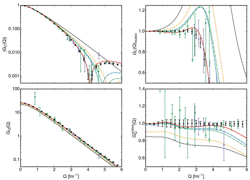
Figure 6: (Color online) Convergence of the chiral expansion for the charge (upper panel) and quadrupole (lower panel) deuteron FFs for the cutoff $\Lambda=500$ MeV. The curves correspond to different chiral orders, namely, black dotted (LO), yellow dashed (NLO), green dot-dashed (N²LO), blue long-dashed (N³LO) and red solid (N⁴LO). For remaining notation see Fig. 5.

We start from the discussion of the chiral expansion for the deuteron form factors which is important for the truncation error estimate. The convergence pattern of the chiral expansion for the charge and quadrupole deuteron form factors is shown in Fig. 6 for the cutoff $\Lambda=500$ MeV. Up to and including N³LO, the calculation does not involve any free parameters, while at N⁴LO, two linear combinations of the LEC’s are adjusted to achieve an overall best description of the deuteron FFs in the range of $Q$-values up to 6 fm^-1. As a general pattern, the chiral expansion of both form factors converges quite well.

For a given value of the cutoff $\Lambda$, truncation errors can be estimated from the convergence pattern of the chiral expansion using the algorithm formulated in Ref. Epelbaum:2014efa . This simple approach has, however, a disadvantage of not directly providing a statistical interpretation of the estimated errors. We therefore follow here the Bayesian approach developed in Refs. Furnstahl:2015rha ; Melendez:2017phj ; Wesolowski:2018lzj ; Melendez:2019izc , which allows one to estimate truncation errors for a given degree-of-belief (DoB) interval. Throughout this analysis, we employ the Bayesian model $\bar{C}_{0.5-10}^{650}$ specified in Ref. Epelbaum:2019zqc and assume the characteristic momentum scale $p$ that determines the expansion parameter

$$q=\max\left(\frac{p}{\Lambda_{b}},\,\frac{M_{\pi}^{\rm eff}}{\Lambda_{b}}\right)$$ (69)

to be given by $|\bm{k}|/2$ Phillips:2006im . In the impulse approximation valid up-to-and-including N²LO, it is easy to see that the deuteron wave function is being probed at the momentum $|\bm{k}|/2$ rather than $|\bm{k}|$, see Ref. Phillips:2006im for a discussion. The quantity $M_{\pi}^{\rm eff}$ in Eq. (69) serves to model the expansion of few-nucleon observables around the chiral limit, while $\Lambda_{b}$ denotes the breakdown scale of chiral EFT.

In Fig. 5, we show the charge and quadrupole FFs calculated at N⁴LO for the cutoff $\Lambda=500$ MeV along with the truncation error corresponding to the $68\%$ degree-of-belief (DOB) interval estimated using Eq. (21) from Epelbaum:2019zqc with $h=10$, $c_{<}=0.5$ and $c_{>}=10$ and assuming $\Lambda_{b}=650$ MeV and $M_{\pi}^{\rm eff}=200$ MeV Epelbaum:2019wvf .

The truncation errors for the structure radius and the quadrupole moment given in Table 1 are estimated in exactly the same way. To make this uncertainty estimate conservatively the truncation error in these quantities is, like in the deuteron FFs, included twice: (i) by performing the Bayesian analysis for $r_{\rm str}^{2}$ and $Q_{d}$ explicitly and (ii) through the statistical uncertainty in the short-range charge density extracted from the fit to $G_{\text{C}}^{\text{exp}}(Q^{2})$ and $G_{\text{Q}}^{\text{exp}}(Q^{2})$ using Eqs. (58) and (59). We also provide in Table 2 the results for the deuteron structure radius and the quadrupole moment at different orders of the chiral expansion along with the corresponding truncation errors, which show a rather natural pattern of convergence for the considered cutoff value of $\Lambda=500$ MeV.

Table 2: Convergence pattern of the chiral expansion and the truncation errors for the deuteron structure radius and the quadrupole moment. All results are obtained for the cutoff $\Lambda=500$ MeV and $Q_{\text{max}}=6$ fm^-1. Truncation errors for $r_{\text{str}}$ are recalculated from errors estimated for $r_{\text{str}}^{2}$ using the Bayesian approach as described in this Section.

	LO	NLO	N2LO	N3LO	N4LO
$r_{\text{str}}^{2}$ [fm2]	$3.8\pm 1.4$	$3.86\pm 0.13$	$3.873\pm 0.029$	$3.877\pm 0.008$	$3.8925\pm 0.0030$
$r_{\text{str}}$ [fm]	$1.9\pm 0.4$	$1.96\pm 0.03$	$1.968\pm 0.007$	$1.9689\pm 0.0019$	$1.9729\pm 0.0008$
$Q_{d}$ [fm2]	$0.24\pm 0.10$	$0.26\pm 0.01$	$0.282\pm 0.006$	$0.2854\pm 0.0017$	$0.2854\pm 0.0005$

VII.5.2 Uncertainty from parametrizations of the nucleon form factors

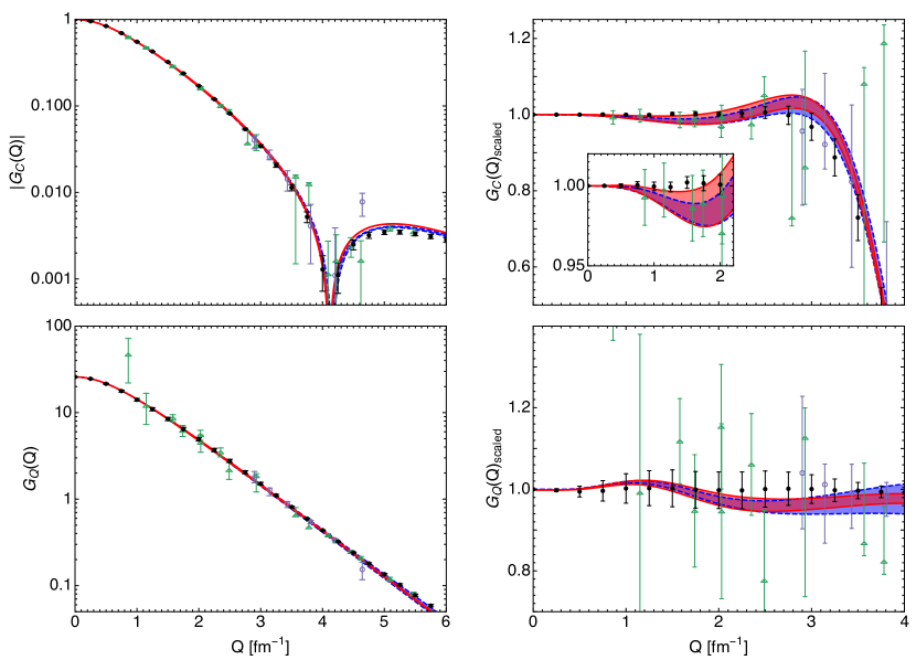
Figure 7: (Color online) Effect of the uncertainty from various parametrizations of the nucleon form factors (see Fig. 4) on the deuteron charge (upper panel) and quadrupole (lower panel) FFs. Red bands (between two solid lines) correspond to the nucleon FFs extracted from the analysis of Ref. Ye:smallrp ; blue bands (between the dashed line) based on the nucleon FFs from Ref. Belushkin:2006qa . For remaining notation see Fig. 5.

In Fig. 7, we demonstrate the effect of the uncertainties from the nucleon FFs on the deuteron charge and quadrupole FFs. Our central results, as given by red bands (between solid lines) in Fig. 7, rely on the nucleon FFs extracted from a recent global analysis of electron scattering data on H, ²H and ³He targets carried out in Refs. Ye:smallrp ; Ye:2017gyb using the proton charge radius from CODATA-2018 as input, see Sec. III.2 for details. The uncertainty from the nucleon FFs, as given in Ref. Ye:smallrp , is included in the statistical uncertainty of our calculation, see Eq. (59).

To investigate the sensitivity of the results to parametrizations of the nucleon FFs, we refitted $G_{\text{C}}(Q^{2})$ and $G_{\text{Q}}(Q^{2})$ using the nucleon FFs from the dispersive analysis of Ref. Belushkin:2006qa (the SC approach), where constraints from unitarity and analyticity were included. The results are shown as blue bands between dashed lines in Fig. 7. On the one hand, the results obtained using the parametrizations of Ref. Ye:smallrp and Ref. Belushkin:2006qa are generally consistent with each other as one may already expect from the comparison of the isoscalar nucleon FFs in Fig. 4. On the other hand, the range where the calculated deuteron FFs appear to be especially sensitive to the details of the nucleon FFs corresponds to the intermediate momentum transfers of $Q\simeq 1-2.5$ fm^-1. In this range, the errors related to the truncation of the chiral expansion are still very small, which can be used to test the consistency of the employed up-to-date nucleon FFs with the deuteron FFs. In the regime of intermediate momenta, $G_{\text{C}}(Q^{2})$ based on the one-nucleon input from Ref. Belushkin:2006qa is systematically lower than that for the nucleon FFs from Ref. Ye:smallrp . This can be seen from Fig. 7 especially if one compares the theoretical results with the parametrization from Refs. Marcucci:2015rca ; Sick:priv : red bands based on the nucleon FFs from Ref. Ye:smallrp are essentially consistent with this parametrization while the blue bands between dashed lines lie systematically lower. This might be related to the fact that the analysis of Ref. Belushkin:2006qa was done before the new high-precision data from Mainz Bernauer:2010wm ; Bernauer:2013tpr have become available. Meanwhile, the updated versions of the dispersive approach Lorenz:2012tm ; Lorenz:2014yda including the MAMI data produce larger values for the proton electric and magnetic FFs at small and intermediate momenta and, as shown in Fig. 3, are in a good agreement with the analysis of Ref. Ye:smallrp . Since the results of Refs. Lorenz:2012tm ; Lorenz:2014yda are given without errors and no updates for a combined dispersive analysis of the proton and neutron FFs was provided in Ref. Lorenz:2014yda , we refrain from using these results in the current investigation.

It is important to emphasize that our results for the structure radius and, therefore, also for the neutron charge radius are only very weakly sensitive to the details of the nucleon FFs used in the fits. This can be understood as follows. The quality of the fits to the world data for the deuteron charge form factor (at least for $Q_{\text{max}}\sim 4$ fm^-1 and higher) increases significantly if the momentum-transfer range around $Q\sim 4$ fm^-1, where $G_{\text{C}}$ becomes small and changes its sign, is well reproduced. Therefore, the contact interaction in the charge density at N⁴LO is adjusted predominantly to reproduce this area. Meanwhile, the comparison of Figs. 5 and 7 reveals that by far the largest source of the uncertainty at $Q\sim 4$ fm^-1 stems from the truncation of the chiral expansion while the nucleon FFs in this $Q$-range have only a minor impact on the statistical uncertainty. Therefore, the structure radius is insensitive to the choice of the parametrization of the nucleon FFs.

VII.5.3 Statistical uncertainty of the LECs determined from $\pi$N and NN data

The chiral SMS NN potential involves two groups of LECs: (i) the $\pi$N LECs from the Roy-Steiner analysis of Ref. Hoferichter:2015tha ; Hoferichter:2015hva , and (ii) the 2N LECs and $\pi$N coupling constants, which are adjusted to achieve the best fit of the neutron-proton and proton-proton scattering data in Ref. Reinert:2020mcu . We consider uncertainties coming from each group.

To account for the statistical uncertainty of the $\pi$N LECs from the Roy-Steiner analysis, we generated a sample of 50 N⁴LO⁺ NN potentials with normally distributed $\pi$N LECs. Then, the propagation of this uncertainty is performed through the variation in the deuteron wave functions. By re-fitting the deuteron FF data we, therefore, extracted the impact of this uncertainty on $r_{\rm str}^{2}$ and $Q_{d}$, as shown in Table 1. The resulting uncertainty from these $\pi$N LECs appears to be very small.

The errors from the statistical uncertainty in the 2N LECs and $\pi$N coupling constants extracted in Ref. Reinert:2020mcu were also propagated to $r_{\rm str}^{2}$ and $Q_{d}$ and the corresponding results are given in Table 1. These errors correspond to the maximum deviations from the central values of $r_{m}$ and $Q_{0}$, which are compatible with the variation of the $\chi^{2}$ in the range $[\chi^{2}_{\text{min}},\chi^{2}_{\text{min}}+1]$ for the description of the neutron-proton and proton-proton data as done in Ref. Reinert:2020mcu . This approach is similar to what was used to estimate the uncertainties of the asymptotic deuteron wave function normalization $A_{S}$ and the ${}^{1}S_{0}$ NN scattering length in Ref. Reinert:2017usi . Note also that in the present work, the method of error propagation from 2N LECs is different from what was done in Ref. Filin:2019eoe , where a covariance matrix was used. We found that the covariance-matrix approach overestimates the corresponding uncertainties for $r_{\rm str}^{2}$. For the deuteron quadrupole moment, however, both approaches give very similar error estimates.

VII.5.4 $Q$-range dependence

As long as the truncation error is included in the uncertainty employed in the fitting procedure, as done in Eq. (59), all data available can, in principle, be included in the fits. This procedure allows us to utilize the deuteron data in the range of $Q$ up to $Q_{\text{max}}=6$ fm^-1 and even higher. The effective weight of the data points at higher transferred momenta is reduced as compared to data points with similar experimental errors at lower $Q$ because the truncation error increases with growing values of $Q$. To estimate (conservatively) the error for the extracted deuteron quantities related with the truncation of the $Q$-range in the fits, we consider the variation of $Q_{\text{max}}$ from $3$ fm^-1 to $7$ fm^-1 and include this error in the uncertainty budget, as shown in Table 1. The results for both $r_{\rm str}^{2}$ and $Q_{d}$ appear to be quite stable to this variation.

VII.5.5 Consistency checks

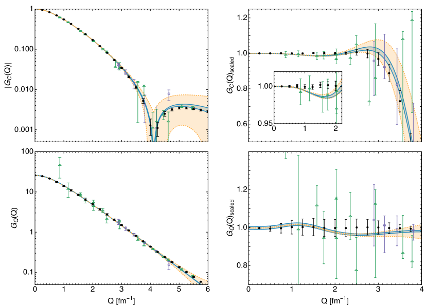
Figure 8: (Color online) Residual cutoff dependence versus the truncation error for the deuteron charge and quadrupole FFs at N⁴LO. Light-shaded blue bands between two solid lines correspond to the cutoff variation in the range of $\Lambda=400\ldots 550$ MeV. For remaining notation see Fig. 5.

We are now in the position to perform several consistency checks of our calculations.

As already pointed out in Sec. III.3, the two-body charge density from OPE is proportional to unobservable unitary-transformation parameters $\bar{\beta}_{8}$ and $\bar{\beta}_{9}$. The observables must be independent of these parameters at least approximately, i.e. up to higher order effects. The results presented above are based on the minimal nonlocality choice, Eq. (27), which is consistent with the employed chiral NN potentials of Ref. Reinert:2020mcu and also with their predecessors from Ref. Reinert:2017usi . To check the sensitivity of the deuteron FFs to $\bar{\beta}_{8}$ and $\bar{\beta}_{9}$, we developed an approximately phase-equivalent version of the 2N potential using a different choice of the unobservable phases, namely $\bar{\beta}_{8}=\bar{\beta}_{9}=1/2$, by re-doing the fit of NN data using exactly the same protocol as in Ref. Reinert:2020mcu . For this particular choice of $\bar{\beta}_{8}$, $\bar{\beta}_{9}$, the OPE contribution to the charge density vanishes exactly: $\rho^{1\pi}_{\text{2N}}=0$. Repeating the fits of the calculated deuteron FFs to the world data, we find for the central values

$$r_{\rm str}^{2}=3.8926\ \text{fm}^{2},\quad\quad Q_{d}=0.2849\ \text{fm}^{2},$$ (70)

which should be compared with the values in Table 1. As expected, the dependence on $\bar{\beta}_{8}$ and $\bar{\beta}_{9}$ for $r_{\rm str}^{2}$ turns out to be very small, that is much smaller than the truncation error of the chiral expansion at N⁴LO. For the quadrupole moment, the dependence on these parameters is also consistent with the truncation error. Note that to achieve the independence of $\bar{\beta}_{8}$, $\bar{\beta}_{9}$ to such a high degree, we found it to be crucial for the nucleon FFs to be included not only in the one-body but also in the two-nucleon OPE charge density. This can be understood as follows: as discussed in Sec. III.3, the derivation of the two-nucleon charge density operators relies on taking the commutator of the leading one-body charge density with the generators of the unitary transformation. Because the one-body density is proportional to the nucleon FF, the same should also hold for the two-body densities. If one neglects the nucleon FFs in the OPE charge density, a sizable violation of the $\bar{\beta}_{8}$, $\bar{\beta}_{9}$ independence would immediately reveal itself in the deuteron quantities. Specifically, in this case one gets $r_{\rm str}^{2}=3.8825\ \text{fm}^{2}$ and $Q_{d}=0.2804\ \text{fm}^{2}$, and one sees that the difference with the values given in Table 1 exceeds the truncation error significantly. The effect on these quantities of neglecting the nucleon FFs in the short-range two-body charge-density operator at N⁴LO is of basically the same size. Also, we would like to emphasize that to observe $\bar{\beta}_{8}$, $\bar{\beta}_{9}$ independence in a large range of momentum transfers it is important to follow the procedure, as described above: first, construct the phase-equivalent NN potentials for some choice of $\bar{\beta}_{8}$, $\bar{\beta}_{9}$ by fitting NN data and then calculate corresponding deuteron wave functions. If one applies the unitary transformation to the existing wave function, then the unitary equivalence will hold only at small momentum transfers, as shown in Ref. Adam:1993zz .

Since the chiral expansion for the deuteron FFs is expected to converge more rapidly for not too soft values of the cutoffs, our central results are obtained for the cutoff $\Lambda=500$ MeV, for which we also carried out a detailed error analysis as described in the previous sections. In Fig. 8, as a consistency check, we confront the cutoff dependence of $G_{\text{C}}(Q)$ and $G_{\text{Q}}(Q)$ from the variation of the cutoff from 400 to 550 MeV with the truncation error. We conclude that for $G_{\text{C}}(Q)$, the cutoff dependence lies well within the truncation error, while for the quadrupole FF they are essentially compatible with each other except for the region of small $Q$ where the cutoff dependence is a little larger. We remind the reader, that the truncation error corresponds to the $68\%$ DOB interval.

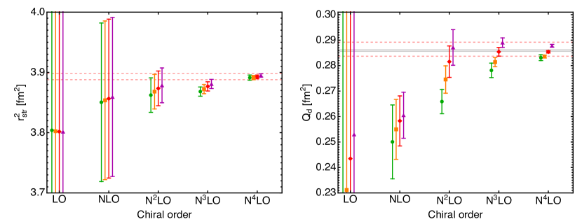
Figure 9: (Color online) Convergence of the chiral expansion for the deuteron structure radius squared (left panel) and the quadrupole moment (right panel). Error bars correspond to the truncation errors in a given chiral order. Green circles stand for the results for $\Lambda=400$ MeV, orange squares for $\Lambda=450$ MeV, red diamonds for $\Lambda=500$ MeV, and purple triangles for $\Lambda=550$ MeV. The band bounded by solid horizontal gray lines on the right panel correspond to the quadrupole moment extracted in Refs. Ericson:1982ei ; Bishop:1979zz . The bands bounded by the dashed horizontal red lines on both panels correspond to the total uncertainties of our central results as given in Table 1.

In Fig. 9, we show the convergence pattern of the chiral expansion for $r_{\rm str}^{2}$ and $Q_{d}$ along with the truncation errors and the cutoff dependence. While the results for $r_{\rm str}^{2}$ converge quite rapidly for any cutoff value, the quadrupole moment, in line with the discussion above, shows a lower rate of convergence. We further emphasize that the uncertainty of our result for the quadrupole moment at the highest considered order is dominated by the statistical errors in the NN LECs and by the uncertainty associated with the choice of the $Q$-range in the fit. Both of these error sources are considerably larger than the truncation uncertainty.

VII.6 Role of the individual contributions at N⁴LO

The role of the individual charge density contributions to the deuteron charge and quadrupole form factors calculated at N⁴LO can be seen in Tables 3 and 4. Unlike the results in Fig. 6, which illustrate the convergence of the chiral expansion, all contributions in Tables 3 and 4 were evaluated using the deuteron wave function at N⁴LO⁺. The results for the one-pion-exchange charge density were obtained using the minimal nonlocality choice for the parameters $\bar{\beta}_{8}$ and $\bar{\beta}_{9}$ from Eq. (27). For the charge FF, the most important correction beyond the main one stems from the CT contribution which dominates in the whole domain of momenta $Q$ considered apart from the region of small $Q$ ($\lesssim$ 1 fm^-1), where the Darwin term is equally important. Next in importance are the $1\pi$ and boost corrections which, however, cancel each other to a large extent. The contribution from the SO is basically negligible. For the quadrupole FF at low $Q$ ($\lesssim$ 1 fm^-1), the dominant corrections beyond the main term originate from the $1\pi$, CT and SO contributions, in the order of their importance, where the first two interfere constructively while the SO is destructive. While the boost correction is negligible for all $Q$-values, the Darwin term, being negligible at small momentum transfers, provides a sizable contribution for $Q>1$ fm.

Table 3: Impact of the individual contributions to the charge density operator on the charge form factor of the deuteron $G_{\text{C}}(Q^{2})$ at N⁴LO for the cutoff $\Lambda=500$ MeV.

Q [fm-1]	Main	SO	Darwin	Boost	$1\pi$	CT	Full
$0.0$	$1.0000$	$0.0000$	$0.0000$	$0.0000$	$0.0000$	$0.0000$	$1.0000$
$0.5$	$0.8416$	$0.0001$	$-0.0012$	$0.0001$	$-0.0004$	$-0.0005$	$0.8397$
$1.0$	$0.5556$	$0.0002$	$-0.0031$	$0.0006$	$-0.0015$	$-0.0017$	$0.5501$
$2.0$	$0.1795$	$0.0004$	$-0.0040$	$0.0018$	$-0.0034$	$-0.0047$	$0.1696$
$3.0$	$0.0460$	$0.0003$	$-0.0023$	$0.0019$	$-0.0034$	$-0.0062$	$0.0363$
$4.0$	$0.0087$	$0.0002$	$-0.0008$	$0.0012$	$-0.0023$	$-0.0056$	$0.0014$
$5.0$	$0.0004$	$0.0001$	$-0.0001$	$0.0005$	$-0.0011$	$-0.0041$	$-0.0043$
$6.0$	$-0.0007$	$0.0000$	$0.0001$	$0.0001$	$-0.0004$	$-0.0026$	$-0.0034$

Table 4: Impact of the individual contributions to the charge density operator on the quadrupole form factor of the deuteron ($G_{\text{Q}}(Q^{2})/m_{d}^{2}$) at N⁴LO for the cutoff $\Lambda=500$ MeV. The values are given in fm².

Q [fm-1]	Main	SO	Darwin	Boost	$1\pi$	CT	Full
$0.0$	$0.2788$	$-0.0018$	$0.0000$	$0.0000$	$0.0063$	$0.0022$	$0.2854$
$0.5$	$0.2340$	$-0.0017$	$-0.0003$	$-0.0001$	$0.0059$	$0.0021$	$0.2399$
$1.0$	$0.1537$	$-0.0013$	$-0.0008$	$-0.0003$	$0.0050$	$0.0019$	$0.1582$
$2.0$	$0.0509$	$-0.0006$	$-0.0011$	$-0.0001$	$0.0027$	$0.0013$	$0.0531$
$3.0$	$0.0151$	$-0.0002$	$-0.0008$	$0.0001$	$0.0011$	$0.0007$	$0.0161$
$4.0$	$0.0043$	$-0.0001$	$-0.0004$	$0.0001$	$0.0004$	$0.0004$	$0.0048$
$5.0$	$0.0012$	$0.0000$	$-0.0002$	$0.0001$	$0.0001$	$0.0002$	$0.0014$
$6.0$	$0.0003$	$0.0000$	$-0.0001$	$0.0001$	$0.0000$	$0.0001$	$0.0004$

VIII Summary and conclusions

In spite of the extensive progress in the understanding of the deuteron structure that has been achieved since more than 50 years, there is still strong motivation to reanalyze the deuteron form factors in the framework of chiral EFT. Being largely governed by the leading-order single-nucleon charge density, the charge and quadrupole deuteron form factors (FFs) are qualitatively described in most of the calculations reported in the literature (at least in some range of the momentum transfer). However, as long as higher-order corrections are concerned, the existing calculations show lack of systematics, consistency and controlled error estimate.

In this paper, the deuteron charge and quadrupole form factors are calculated using consistently regularized two-nucleon potentials and the charge density in chiral effective field theory. This allowed to extract the important static properties of the deuteron, namely the structure radius and the quadrupole moment, with unprecedented accuracy and to reliably estimate various sources of uncertainty. Our analysis provides a first step towards the understanding of radii of medium-mass and heavy nuclei, which are currently known to be significantly underpredicted.

The novel aspects of our study include:

• For the first time, the calculation of the deuteron FFs is pushed beyond N³LO, which allows one to reduce the uncertainty from the truncation of chiral expansion and thus to extend the range of momenta considered. To achieve this goal we (i) employed the most recent two-nucleon potentials up through N⁴LO⁺ Reinert:2020mcu , which utilize a complete treatment of isospin-breaking effects and provide a statistically perfect description of NN data below pion production threshold and (ii) implemented the charge density operator at N³LO, supplemented with the 2N short-range operators at N⁴LO.

• Regularization of the charge density operators is carried out consistently with the two-nucleon potential using the same unitarity transformations for the charge density operators and the nuclear forces. Specifically, the two-nucleon charge density operators are generated by taking the commutator of the leading one-body charge density with the generators of the unitary transformation that incorporate the regulator as discussed in Sec. III.3. As a consistency check, we have demonstrated that the residual cutoff dependence of the deuteron charge FF and the extracted structure radius is much weaker than the error estimated from the truncation of the chiral expansion at N⁴LO. The cutoff dependence of the quadrupole moment (and in general of the quadrupole FF at low $Q$) at the highest considered order is somewhat larger than the estimated truncation error, but still of the same size as the total uncertainty of our result. Furthermore, the short-range charge density operators contributing to the charge and quadrupole FFs of the deuteron come out of a natural size.

• Instead of relying on the strict chiral expansion of the nucleon FFs known to converge slowly, we employed the most up-to-date phenomenological parametrizations of experimental data from the global analysis of Refs. Ye:2017gyb ; Ye:smallrp . The nucleon form factors from the dispersive approach of Ref. Belushkin:2006qa have also been used as a consistency check. We emphasize that making a reliable calculation of the deuteron FFs requires the inclusion of the nucleon FFs both in the one- and two-nucleon charge density operators, the feature that becomes obvious in the way we generate the two-body charge density by means of the unitary transformation. We have verified this conclusion by explicitly checking the insensitivity of our results for the FFs to the choice of unobservable unitary phases $\bar{\beta}_{8}$ and $\bar{\beta}_{9}$, which holds true to a very high degree of accuracy when keeping the nucleon FFs in the OPE charge density. The same conclusion applies when the nucleon FFs are neglected in the contact two-nucleon charge density at N⁴LO.

• A comprehensive and systematic analysis of various sources of uncertainties in the calculated deuteron FFs is performed. Specifically, we estimated the uncertainty from (i) propagating the statistical errors of the $\pi$N and NN low-energy constants (LECs) entering the two-nucleon potentials (ii) truncation of the chiral expansion evaluated using Bayesian methods (iii) statistical uncertainties in the N⁴LO short-range charge density operators, (iv) employed parametrizations of the nucleon FFs and (v) fixing the maximum value of the momentum transfers $Q_{\text{max}}$ in the fits of the short-range charge operators.

Pushing the calculation to N⁴LO and using the consistently regularized charge density operators together with the phenomenological nucleon form factors is found to result in a very good description of the deuteron form factors at least up to $Q\simeq 6$ fm^-1. Having adjusted the two short-range operators to achieve the best fit of the world data on the charge and quadrupole FFs of the deuteron, we predict the deuteron structure radius and quadrupole moment to have the values of

$$r_{\rm str}=1.9729\begin{subarray}{c}+0.0015\\ -0.0012\end{subarray}\ \text{fm},\quad\quad Q_{d}=0.2854\begin{subarray}{c}+0.0038\\ -0.0017\end{subarray}\ \text{fm}^{2}.$$ (71)

Equipped with this prediction for the structure radius, we employ the high-accuracy data for the hydrogen-deuterium isotope shift in Eq. (53) to extract the mean-square neutron charge radius, for which we obtain

$$r_{n}^{2}=-0.105\begin{subarray}{c}+0.005\\ -0.006\end{subarray}\ \text{fm}^{2}.$$ (72)

This result is consistent with our previous determination in Ref. Filin:2019eoe but deviates by about $1.9\sigma$ from the current value $r_{n}^{2}=-0.1161(22)\text{ fm}^{2}$ given by the Particle Data Group Tanabashi:2018oca and deviates by about $1.4\sigma$ from the very recent determination $r_{n}^{2}=-0.122\pm 0.004_{\rm(stat.)}\pm 0.010_{\rm(syst.)}$ fm² from the collective analysis of the nucleon form factors of Ref. Atac:2020hdq .

Appendix A Analytic expressions for the contributions to $G_{\text{C}}$, $G_{\text{Q}}$, $r_{\text{str}}^{2}$ and $Q_{d}$.

In this appendix we list the analytic expressions for individual contributions to the deuteron charge form factor $G_{\text{C}}$ (Eq. (46)), quadrupole form factor $G_{\text{Q}}$ (Eq. (54)), structure radius squared $r_{\text{str}}^{2}$ (Eqs. (52), (49)) and quadrupole moment $Q_{d}$ (Eq. (56)). Results are given in momentum space or in coordinate space depending on which form is simpler for practical calculations. All contributions are grouped according to the charge density operator which they are obtained from. Specifically, we distinguish the following types of contributions: main (LO) contributions, Darwin-Foldy-type contributions, spin-orbit corrections, deuteron boost corrections, pion-exchange current contributions, and contact contributions. Results are expressed in terms of deuteron wave functions and single-nucleon form factors. The deuteron WFs are normalized according to:

$$\int\limits_{0}^{\infty}p^{2}\left({u(p)}^{2}+{w(p)}^{2}\right)dp=\int\limits_{0}^{\infty}\left({u(r)}^{2}+{w(r)}^{2}\right)dr=1,$$ (73)

and the deuteron $D$-state probability is:

$$P_{D}=\int\limits_{0}^{\infty}p^{2}{w(p)}^{2}dp=\int\limits_{0}^{\infty}{w(r)}^{2}dr.$$ (74)

We also introduce the following common combinations of the deuteron wave functions:

$$C(r)\equiv u^{2}(r)+w^{2}(r),\qquad Q(r)\equiv u(r)w(r)-\frac{w^{2}(r)}{\sqrt{8}}.$$ (75)

Note that all momenta in this section are three-dimensional. For a vector $\bm{x}$, we use $x$ to denote $x\equiv|\bm{x}|$.

A.1 Main (LO) contributions

Main contributions stem from the LO charge density operator in Eq. (24);

$$G_{\text{C}}^{\text{Main}}(\bm{k}^{2})=G_{\text{E}}^{S}(\bm{k}^{2})G_{\text{C}}^{\text{matter}}(\bm{k}^{2}),\qquad G_{\text{Q}}^{\text{Main}}(\bm{k}^{2})=G_{\text{E}}^{S}(\bm{k}^{2})G_{\text{Q}}^{(0)}(\bm{k}^{2}),$$ (76)

where we introduced the following auxiliary functions:

$$G_{\text{C}}^{\text{matter}}(\bm{k}^{2})\equiv\int_{0}^{\infty}C(r)j_{0}\left(\frac{kr}{2}\right)dr,\qquad\qquad G_{\text{Q}}^{(0)}(\bm{k}^{2})\equiv\frac{6\sqrt{2}m_{d}^{2}}{\bm{k}^{2}}\int_{0}^{\infty}Q(r)j_{2}\left(\frac{kr}{2}\right)dr.$$ (77)

The LO contribution to the deuteron structure radius (so called deuteron matter radius) reads:

$$r_{m}^{2}=r_{0}^{2}=\frac{1}{4}\int\limits_{0}^{\infty}\left(p^{2}\left(u^{\prime}{(p)}^{2}+w^{\prime}{(p)}^{2}\right)+6w{(p)}^{2}\right)dp=\frac{1}{4}\int_{0}^{\infty}\left({u(r)}^{2}+{w(r)}^{2}\right)r^{2}dr.$$ (78)

The LO contribution to the deuteron quadrupole moment reads:

$$Q_{0}=\int\limits_{0}^{\infty}\left(\frac{p^{2}u^{\prime}(p)w^{\prime}(p)}{5\sqrt{2}}-\frac{1}{20}p^{2}w^{\prime}{(p)}^{2}+\frac{3pw(p)u^{\prime}(p)}{5\sqrt{2}}-\frac{3{w(p)}^{2}}{10}\right)dp=\frac{\sqrt{2}}{10}\int_{0}^{\infty}Q(r)r^{2}dr.$$ (79)

A.2 Darwin-Foldy-type of contributions

The Darwin-Foldy-type (DF) of contributions stem from the charge density operator $\rho_{\text{1N}}^{\text{DF}}$ in Eq. (24). Since the DF charge density operator differs from the LO operator only by a pre-factor, the resulting DF contributions to the form factors are trivially related to the LO ones. Specifically, the DF contributions to the deuteron charge and quadrupole form factors read:

$$G_{\text{C}}^{\text{DF}}(\bm{k}^{2})=G_{\text{E}}^{S}(\bm{k}^{2})\left(-\frac{\bm{k}^{2}}{8m_{N}^{2}}\right)G_{\text{C}}^{\text{matter}}(\bm{k}^{2}),\qquad\qquad G_{\text{Q}}^{\text{DF}}(\bm{k}^{2})=G_{\text{E}}^{S}(\bm{k}^{2})\left(-\frac{\bm{k}^{2}}{8m_{N}^{2}}\right)G_{\text{Q}}^{(0)}(\bm{k}^{2}).$$ (80)

Deuteron structure radius does, by definition, exclude the Darwin-Foldy contribution, but the deuteron charge radius receives a constant correction $r_{DF}^{2}=3/(4m_{p}^{2})=0.03317\,\text{fm}^{2}$, where $m_{p}$ is a proton mass. Finally, the Darwin-Foldy term does not contribute to the deuteron quadrupole moment since it is proportional to the photon momentum $k$, while the quadrupole moment is defined at $k=0$.

A.3 Spin-orbit contributions

The spin-orbit contributions to the deuteron form factors stemming from the charge density operator $\rho_{\text{1N}}^{\text{SO}}$ of Eq. (24) read:

$$G_{\text{C}}^{\text{SO}}(\bm{k}^{2})=\left(G_{\text{E}}^{S}(\bm{k}^{2})-2G_{\text{M}}^{S}(\bm{k}^{2})\right)G_{\text{C}}^{\text{ang}}(\bm{k}^{2}),\qquad\qquad G_{\text{Q}}^{\text{SO}}(\bm{k}^{2})=\left(G_{\text{E}}^{S}(\bm{k}^{2})-2G_{\text{M}}^{S}(\bm{k}^{2})\right)G_{\text{Q}}^{\text{ang}}(\bm{k}^{2}),$$ (81)

where

$$G_{\text{C}}^{\text{ang}}(\bm{k}^{2})\equiv\frac{3}{2m_{N}^{2}}\int_{0}^{\infty}\frac{{w(r)}^{2}}{r}\frac{\partial}{\partial r}\left(j_{0}\left(\frac{kr}{2}\right)\right)dr=-\frac{3k}{4m_{N}^{2}}\int_{0}^{\infty}\frac{{w(r)}^{2}}{r}j_{1}\left(\frac{kr}{2}\right)dr,$$ (82)

$$G_{\text{Q}}^{\text{ang}}(\bm{k}^{2})\equiv(-1)\frac{6}{\sqrt{2}\bm{k}^{2}}\frac{3m_{d}^{2}}{m_{N}^{2}}\int_{0}^{\infty}w(r)\left(\frac{\partial}{\partial r}\left(\frac{u(r)}{r}\right)-\frac{1}{\sqrt{2}}\frac{1}{r}\frac{\partial w(r)}{\partial r}\right)j_{2}\left(\frac{kr}{2}\right)dr.$$ (83)

The corresponding contributions to the deuteron structure radius and quadrupole moment read:

$$r_{\text{SO}}^{2}=-\frac{3}{4m_{N}^{2}}(2\mu_{n}+2\mu_{p}-1)P_{D},\qquad Q_{\text{SO}} = (1-2\mu_{n}-2\mu_{p})Q_{\text{angular}},$$ (84)

where $\mu_{p}$ and $\mu_{n}$ are the magnetic moments of the proton and the neutron, respectively, in units of nuclear magnetons, and

$$Q_{\text{angular}}\equiv(-1)\frac{6}{\sqrt{2}}\frac{3}{m_{N}^{2}}\int_{0}^{\infty}w(r)\left(\frac{\partial}{\partial r}\left(\frac{u(r)}{r}\right)-\frac{1}{\sqrt{2}}\frac{1}{r}\frac{\partial w(r)}{\partial r}\right)\frac{r^{2}}{60}dr.$$ (85)

A.4 Boost corrections

Corrections to the deuteron form factors which appear due to the motion of initial and final deuterons are discussed in the Section V. The final expressions for the boost corrections to the charge and quadrupole form factors have the form:

$$G_{\text{C}}^{\text{Boost}}(\bm{k}^{2}) = G_{\text{E}}^{S}(\bm{k}^{2})G_{\text{C}}^{\text{ang}}(\bm{k}^{2})+G_{\text{E}}^{S}(\bm{k}^{2})\left(G_{\text{C}}^{\text{matter}}(\bm{k}_{\text{boosted}}^{2})-G_{\text{C}}^{\text{matter}}(\bm{k}^{2})\right),$$ (86)

$$G_{\text{Q}}^{\text{Boost}}(\bm{k}^{2}) = G_{\text{E}}^{S}(\bm{k}^{2})G_{\text{Q}}^{\text{ang}}(\bm{k}^{2})+G_{\text{E}}^{S}(\bm{k}^{2})\left(G_{\text{Q}}^{(0)\text{Boosted}}(\bm{k}^{2})-G_{\text{Q}}^{(0)}(\bm{k}^{2})\right),$$ (87)

where the boosted momentum $k_{\text{boosted}}$ is defined by Eq. (45) and the boosted version of $G_{\text{Q}}^{(0)}$ is

$$G_{\text{Q}}^{(0)\text{Boosted}}(\bm{k}^{2})\equiv\frac{6\sqrt{2}m_{d}^{2}}{\bm{k}^{2}}\int_{0}^{\infty}w(r)\left({u(r)}-\frac{w(r)}{2\sqrt{2}}\right)j_{2}\left(\frac{k_{\text{boosted}}r}{2}\right)dr.$$ (88)

Boost corrections do not contribute to the deuteron structure radius and quadrupole moment.

A.5 One-pion-exchange contributions

One-pion-exchange (OPE) contributions to the deuteron form factors originate from the charge density operator given by Eq. (36). In momentum space, the expressions for the OPE contributions involve six-dimensional integration and are somewhat cumbersome. The Fourier transform to coordinate space makes these expressions much shorter and the number of integrations reduces to one. Below we give the OPE contributions in coordinate space. For the sake of compactness, we introduce the functions $\bar{h}_{1}(x)$ and $\bar{h}_{2}(x)$ that correspond to the Fourier transforms of the regularized single and squared pion propagators, respectively:

$$\bar{h}_{1}(r)\equiv\int\frac{d^{3}l}{{(2\pi)}^{3}}\frac{F_{1}(\bm{l}^{2},\Lambda)e^{i\bm{l}\cdot\bm{r}}}{\bm{l}^{2}+M_{\pi}^{2}},\qquad\bar{h}_{2}(r)\equiv\int\frac{d^{3}l}{{(2\pi)}^{3}}\frac{F_{2}(\bm{l}^{2},\Lambda)e^{i\bm{l}\cdot\bm{r}}}{{(\bm{l}^{2}+M_{\pi}^{2})}^{2}},$$ (89)

where $F_{1}(\bm{l}^{2},\Lambda)$ and $F_{2}(\bm{l}^{2},\Lambda)$ are the corresponding momentum-space regulators. Without regularization (i.e. when $F_{1}(\bm{l}^{2},\Lambda)=F_{2}(\bm{l}^{2},\Lambda)=1$), the functions $\bar{h}_{1}(r)$ and $\bar{h}_{2}(r)$ take a simple form:

$$\bar{h}_{1}^{\text{unreg}}(r)=\frac{e^{-M_{\pi}r}}{4\pi r},\qquad\bar{h}_{2}^{\text{unreg}}(r)=\frac{e^{-M_{\pi}r}}{8\pi M_{\pi}}.$$ (90)

For the regulator employed in the SMS NN potentials of Ref. Reinert:2017usi with

$$F^{\text{SMS}}_{1}(\bm{l}^{2},\Lambda)\equiv\exp\left(\frac{\bm{l}^{2}+M_{\pi}^{2}}{\Lambda^{2}}\right),\qquad F^{\text{SMS}}_{2}(\bm{l}^{2},\Lambda)\equiv\exp\left(\frac{\bm{l}^{2}+M_{\pi}^{2}}{\Lambda^{2}}\right)\left[1+\frac{\bm{l}^{2}+M_{\pi}^{2}}{\Lambda^{2}}\right]$$ (91)

we get the following closed form of the function $\bar{h}_{1}(r)$

$$\bar{h}^{\text{SMS}}_{1}(r) = \frac{\exp(-M_{\pi}r)\,\text{erfc}\left(\frac{M_{\pi}}{\Lambda}-\frac{\Lambda r}{2}\right)-\exp(M_{\pi}r)\,\text{erfc}\left(\frac{M_{\pi}}{\Lambda}+\frac{\Lambda r}{2}\right)}{8\pi r}.$$ (92)

The function $\bar{h}_{2}$ enters the final result only under a derivative operator. To simplify the expressions even further we rewrite $\bar{h}^{\prime}_{2}(r)$ in terms of $\bar{h}_{1}(r)$. We employ the relation

$$\frac{\bm{l}}{{(\bm{l}^{2}+M_{\pi}^{2})}^{2}}F_{2}(\bm{l}^{2},\Lambda)=-\frac{1}{2}\bm{\nabla}_{l}\left(\frac{1}{\bm{l}^{2}+M_{\pi}^{2}}F_{1}(\bm{l}^{2},\Lambda)\right),$$ (93)

which is fulfilled by both the unregularized and SMS-regularized pion propagators. Substituting the relation in Eq. (93) in the definition of $\bar{h}_{2}$, taking the derivative and integrating by parts leads to the following relation in coordinate space:

$$\bar{h}_{2}^{\prime}(r)=\left(-\frac{r}{2}\right)\bar{h}_{1}(r).$$ (94)

Using the simplifications above, the OPE contribution to the deuteron charge form factor can be written as:

$$G_{\text{C}}^{1\pi}(\bm{k}^{2}) = G_{\text{E}}^{S}(\bm{k}^{2})\frac{g_{A}^{2}}{16F_{\pi}^{2}m_{N}}\int\limits_{0}^{\infty}dr\Bigg{(}(2\bar{\beta}_{8}-1)kj_{1}\left(\frac{kr}{2}\right)\left(C(r)\left(r\bar{h}_{1}^{\prime\prime}(r)+4\bar{h}_{1}^{\prime}(r)\right)+4\sqrt{2}Q(r)\left(r\bar{h}_{1}^{\prime\prime}(r)+\bar{h}_{1}^{\prime}(r)\right)\right)$$ (95)

$$+(1-2\bar{\beta}_{9})kj_{1}\left(\frac{kr}{2}\right)\left(C(r)+4\sqrt{2}Q(r)\right)\bar{h}_{1}^{\prime}(r)\Bigg{)},$$

where $j_{n}(x)$ are the spherical Bessel functions. The OPE contribution to the deuteron quadrupole form factor reads:

$$G_{\text{Q}}^{1\pi}(\bm{k}^{2}) = G_{\text{E}}^{S}(\bm{k}^{2})\frac{g_{A}^{2}m_{d}^{2}}{16F_{\pi}^{2}m_{N}}\int\limits_{0}^{\infty}dr\Bigg{\{}(2\bar{\beta}_{8}-1)$$ (96)

$$\times\Bigg{(}\frac{36}{k^{2}r}j_{2}\left(\frac{kr}{2}\right)\left(-2C(r)\left(\bar{h}_{1}^{\prime}(r)-r\bar{h}_{1}^{\prime\prime}(r)\right)+\sqrt{2}Q(r)\left(4\bar{h}_{1}^{\prime}(r)-r\bar{h}_{1}^{\prime\prime}(r)\right)+9w{(r)}^{2}\bar{h}_{1}^{\prime}(r)\right)$$

$$-\frac{6}{k}j_{1}\left(\frac{kr}{2}\right)\left(2C(r)\left(r\bar{h}_{1}^{\prime\prime}(r)+\bar{h}_{1}^{\prime}(r)\right)+\sqrt{2}Q(r)\left(2\bar{h}_{1}^{\prime}(r)-r\bar{h}_{1}^{\prime\prime}(r)\right)\right)\Bigg{)}$$

$$+(1-2\bar{\beta}_{9})\left(\frac{324}{k^{2}r}j_{2}\left(\frac{kr}{2}\right)w{(r)}^{2}\bar{h}_{1}^{\prime}(r)-\frac{24}{k}j_{1}\left(\frac{kr}{2}\right)\left(C(r)-\frac{Q(r)}{\sqrt{2}}\right)\bar{h}_{1}^{\prime}(r)\right)\Bigg{\}}.$$

Finally, the OPE contributions to the deuteron structure radius and quadrupole moment have the form:

$$r^{2}_{1\pi} = -\frac{g_{A}^{2}}{16F_{\pi}^{2}m_{N}}\int\limits_{0}^{\infty}dr\,r\Bigg{(}(2\bar{\beta}_{8}-1)\left(C(r)\left(r\bar{h}_{1}^{\prime\prime}(r)+4\bar{h}_{1}^{\prime}(r)\right)+4\sqrt{2}Q(r)\left(r\bar{h}_{1}^{\prime\prime}(r)+\bar{h}_{1}^{\prime}(r)\right)\right)$$ (97)

$$+2(1-2\bar{\beta}_{9})\left(C(r)+4\sqrt{2}Q(r)\right)\bar{h}_{1}^{\prime}(r)\Bigg{)},$$

$$Q^{1\pi} = \frac{g_{A}^{2}}{16F_{\pi}^{2}m_{N}}\frac{1}{5}\int\limits_{0}^{\infty}dr\,r\Bigg{(}(2\bar{\beta}_{8}-1)\left(-4C(r)\left(r\bar{h}_{1}^{\prime\prime}(r)+4\bar{h}_{1}^{\prime}(r)\right)+2\sqrt{2}Q(r)\left(r\bar{h}_{1}^{\prime\prime}(r)+\bar{h}_{1}^{\prime}(r)\right)+27w{(r)}^{2}\bar{h}_{1}^{\prime}(r)\right)$$ (98)

$$-(1-2\bar{\beta}_{9})\bar{h}_{1}^{\prime}(r)\left(20C(r)-10\sqrt{2}Q(r)-27w{(r)}^{2}\right)\Bigg{)}.$$

Our analytic expressions for OPE contributions agree with the ones of Ref. Friar:1979by after the following notational changes are performed:

$$\bar{h}_{1}\to\frac{M_{\pi}}{4\pi}h,\qquad\frac{g_{A}^{2}M_{\pi}^{2}}{16\pi F_{\pi}^{2}}\to f_{0}^{2},\qquad\bar{\beta}_{9}\to\frac{\mu-1}{4}\qquad\bar{\beta}_{8}\to\frac{\nu}{2}.$$ (99)

A.6 Contact charge density contributions

Contact N⁴LO contributions to the deuteron form factors stem from the corresponding short-range charge density operators in Eq. (39). The contact contribution to the deuteron charge form factor is given by

$$G_{\text{C}}^{\text{Cont}}(\bm{k}^{2}) = \frac{1}{\pi^{2}}G_{\text{E}}^{S}(\bm{k}^{2})\int\limits_{0}^{\infty}p^{2}dp\int\limits_{0}^{\infty}p^{\prime 2}dp^{\prime}F_{\Lambda}\left(p-\frac{k}{2},p^{\prime}\right)$$ (100)

$$\times\big{[}F_{G_{\text{C}}}^{uu}(p,p^{\prime},k)u(p)u(p^{\prime})+F_{G_{\text{C}}}^{uw}(p,p^{\prime},k)w(p)u(p^{\prime})\big{]}+(k\to-k),$$

where

$$F_{\Lambda}\left(p,p^{\prime}\right) = \exp\left(-\frac{p^{2}+p^{\prime 2}}{\Lambda^{2}}\right),$$ (101)

$$F_{G_{\text{C}}}^{uu}(p,p^{\prime},k) = \left(A+B+\frac{C}{3}\right)\frac{2}{kp}\left(\Lambda^{4}+\Lambda^{2}\left({\left(p-\frac{k}{2}\right)}^{2}-p^{\prime 2}\right)\right),$$ (102)

$$F_{G_{\text{C}}}^{uw}(p,p^{\prime},k) = \sqrt{2}C\left(\frac{\Lambda^{6}}{kp^{3}}+\frac{\Lambda^{4}\left(4p-3k\right)}{3kp^{2}}+\frac{\Lambda^{2}\left(k-4p\right)}{3p}\right),$$ (103)

and $(k\to-k)$ means that the same contribution, but with opposite sign of $k$ should be added. The contact contribution to the deuteron quadrupole form factor reads

$$G_{\text{Q}}^{\text{Cont}}(\bm{k}^{2})=\frac{m_{d}^{2}}{\pi^{2}}G_{\text{E}}^{S}(\bm{k}^{2})\int\limits_{0}^{\infty}p^{2}dp\int\limits_{0}^{\infty}p^{\prime 2}dp^{\prime}F_{\Lambda}\left(p-\frac{k}{2},p^{\prime}\right)\big{[}F_{G_{\text{Q}}}^{uu}(p,p^{\prime},k)u(p)u(p^{\prime})$$

$$+F_{G_{\text{Q}}}^{uw}(p,p^{\prime},k)w(p)u(p^{\prime})+F_{G_{\text{Q}}}^{ww}(p,p^{\prime},k)w(p)w(p^{\prime})\big{]}+(k\to-k),$$ (104)

where

$$F_{G_{\text{Q}}}^{uu}(p,p^{\prime},k) = (-1)C\frac{\Lambda^{2}}{2k^{5}p}\left(k^{2}{\left(p-\frac{k}{2}\right)}^{2}+k(k-3p)\Lambda^{2}+3\Lambda^{4}\right),$$

$$F_{G_{\text{Q}}}^{uw}(p,p^{\prime},k) = (A+B)\frac{(-3)}{\sqrt{2}k^{5}p^{3}}\Bigg{(}k^{2}p^{2}\left((k-2p)^{2}-4p^{\prime 2}\right)\Lambda^{2}-kp\left(3k^{2}-16kp+12(p^{2}-p^{\prime 2})\right)\Lambda^{4}$$

$$+3\left(k^{2}-12kp+4(p^{2}-p^{\prime 2})\right)\Lambda^{6}+36\Lambda^{8}\Bigg{)}$$

$$+\frac{C}{\sqrt{2}k^{5}p^{3}}\left(k^{2}p^{2}\left({(k-2p)}^{2}+4p^{\prime 2}\right)\Lambda^{2}-kp\left(3k^{2}-4kp+12\left(p^{2}+p^{\prime 2}\right)\right)\Lambda^{4}+3\left(k^{2}+4\left(p^{2}+p^{\prime 2}\right)\right)\Lambda^{6}\right),$$

$$F_{G_{\text{Q}}}^{ww}(p,p^{\prime},k) = C\frac{8p^{\prime 2}\left(k^{2}p^{2}\Lambda^{2}-3kp\Lambda^{4}+3\Lambda^{6}\right)}{k^{5}p^{3}}.$$ (105)

Next, the contact charge density contribution to the deuteron structure radius has the form

$$r^{2}_{\text{Cont}}=\frac{1}{\pi^{2}}\int\limits_{0}^{\infty}p^{2}dp\int\limits_{0}^{\infty}p^{\prime 2}dp^{\prime}F_{\Lambda}\left(p,p^{\prime}\right)\big{[}F_{r^{2}}^{uu}(p,p^{\prime})u(p)u(p^{\prime})+F_{r^{2}}^{uw}(p,p^{\prime})w(p)u(p^{\prime})\big{]},$$ (106)

where

$$F_{r^{2}}^{uu}(p,p^{\prime}) \equiv -2\left(A+B+\frac{C}{3}\right)\left(3-\frac{2(p^{2}+p^{\prime 2})}{\Lambda^{2}}+\frac{{(p^{2}-p^{\prime 2})}^{2}}{\Lambda^{4}}\right),$$ (107)

$$F_{r^{2}}^{uw}(p,p^{\prime}) \equiv \frac{8\sqrt{2}}{3}\,C\,\left(\frac{2p^{2}}{\Lambda^{2}}+\frac{p^{2}\left(p^{\prime 2}-p^{2}\right)}{\Lambda^{4}}\right).$$ (108)

Finally, the contact contribution to the quadrupole moment reads:

$$Q_{\text{Cont}}=\frac{1}{\pi^{2}}\int\limits_{0}^{\infty}p^{2}dp\int\limits_{0}^{\infty}p^{\prime 2}dp^{\prime}F_{\Lambda}\left(p,p^{\prime}\right)\big{[}F_{Q}^{uu}(p,p^{\prime})u(p)u(p^{\prime})+F_{Q}^{uw}(p,p^{\prime})w(p)u(p^{\prime})+F_{Q}^{ww}(p,p^{\prime})w(p)w(p^{\prime})\big{]},$$ (109)

where

$$F_{Q}^{uu}(p,p^{\prime}) \equiv (-4C)\left(1-\frac{2(p^{2}+p^{\prime 2})}{3\Lambda^{2}}+\frac{2(p^{4}+p^{\prime 4})}{15\Lambda^{4}}\right),\qquad F_{Q}^{ww}(p,p^{\prime})\equiv\frac{16}{15}C\frac{p^{2}p^{\prime 2}}{\Lambda^{4}},$$ (110)

$$F_{Q}^{uw}(p,p^{\prime}) \equiv \frac{4\sqrt{2}}{15}p^{2}\left((A+B)\left(\frac{6}{\Lambda^{2}}+\frac{3(p^{\prime 2}-p^{2})}{\Lambda^{4}}\right)+C\left(-\frac{5}{\Lambda^{2}}+\frac{p^{2}+p^{\prime 2}}{\Lambda^{4}}\right)\right).$$ (111)

Appendix B Complete expressions for the contact charge density at N⁴LO including isovector terms

In this appendix we present the N⁴LO contact charge density operators including isovector contributions. The isovector components do not contribute to the deuteron observables in the single-photon approximation, but have to be taken into account when calculating the FFs and charge radii of heavier nuclei. Charge-density operators presented here are derived using the same procedure as used for derivation of Eq. (33), but keeping the isovector terms. After calculating and antisymmetrizing the commutators of the LO charge density with the generators of the unitary transformation Eq. (III.3) we obtain the following result for the N⁴LO contact charge density:

$$\rho_{\text{Cont,AS}}^{(A+B+C/3)} = 2e\left(A+B+\frac{C}{3}\right)\frac{\bm{\sigma}_{1}\cdot\bm{\sigma}_{2}+3}{4}\bigg{[}G_{\text{E}}^{S}(\bm{k}^{2})\frac{1-\bm{\tau}_{1}\cdot\bm{\tau}_{2}}{4}\bm{k}^{2}$$ (112)

$$+G_{\text{E}}^{V}(\bm{k}^{2})\left(\frac{{(\bm{\tau}_{1}-\bm{\tau}_{2})}_{3}}{2}\bm{k}\cdot(\bm{p}-\bm{p}^{\prime})-\frac{i{(\bm{\tau}_{1}\times\bm{\tau}_{2})}_{3}}{2}\bm{k}\cdot(\bm{p}+\bm{p}^{\prime})\right)\bigg{]},$$

$$\rho_{\text{Cont,AS}}^{(A-3B-C)} = 2e\,(A-3B-C)\frac{1-\bm{\sigma}_{1}\cdot\bm{\sigma}_{2}}{4}\bigg{[}\left(G_{\text{E}}^{S}(\bm{k}^{2})\frac{\bm{\tau}_{1}\cdot\bm{\tau}_{2}+3}{4}+G_{\text{E}}^{V}(\bm{k}^{2})\frac{{(\bm{\tau}_{1}+\bm{\tau}_{2})}_{3}}{2}\right)\,\bm{k}^{2}$$ (113)

$$+G_{\text{E}}^{V}(\bm{k}^{2})\left(\frac{{(\bm{\tau}_{1}-\bm{\tau}_{2})}_{3}}{2}\bm{k}\cdot(\bm{p}-\bm{p}^{\prime})+\frac{i{(\bm{\tau}_{1}\times\bm{\tau}_{2})}_{3}}{2}\bm{k}\cdot(\bm{p}+\bm{p}^{\prime})\right)\bigg{]},$$

$$\rho_{\text{Cont,AS}}^{(C)} = 2e\,C\bigg{[}\,G_{\text{E}}^{S}(\bm{k}^{2})\frac{1-\bm{\tau}_{1}\cdot\bm{\tau}_{2}}{4}\left((\bm{k}\cdot\bm{\sigma}_{1})(\bm{k}\cdot\bm{\sigma}_{2})-\frac{1}{3}\bm{k}^{2}(\bm{\sigma}_{1}\cdot\bm{\sigma}_{2})\right)$$

$$+G_{\text{E}}^{V}(\bm{k}^{2})\frac{{(\bm{\tau}_{1}-\bm{\tau}_{2})}_{3}}{2}\frac{1}{2}\left((\bm{k}\cdot\bm{\sigma}_{1})\bm{\sigma}_{2}\cdot(\bm{p}-\bm{p}^{\prime})+(\bm{k}\cdot\bm{\sigma}_{2})\bm{\sigma}_{1}\cdot(\bm{p}-\bm{p}^{\prime})-\frac{2}{3}\bm{k}\cdot(\bm{p}-\bm{p}^{\prime})(\bm{\sigma}_{1}\cdot\bm{\sigma}_{2})\right)$$

$$-G_{\text{E}}^{V}(\bm{k}^{2})\frac{i{(\bm{\tau}_{1}\times\bm{\tau}_{2})}_{3}}{2}\frac{1}{2}\left((\bm{k}\cdot\bm{\sigma}_{1})\bm{\sigma}_{2}\cdot(\bm{p}+\bm{p}^{\prime})+(\bm{k}\cdot\bm{\sigma}_{2})\bm{\sigma}_{1}\cdot(\bm{p}+\bm{p}^{\prime})-\frac{2}{3}\bm{k}\cdot(\bm{p}+\bm{p}^{\prime})(\bm{\sigma}_{1}\cdot\bm{\sigma}_{2})\right)\bigg{]}.$$

Notice that all isoscalar operators are proportional to $G_{\text{E}}^{S}({\bm{k}}^{2})$, while all isovector ones are proportional to $G_{\text{E}}^{V}({\bm{k}}^{2})$.

Finally we would like to make a remark about the ${}^{1}S_{0}\to{}^{1}S_{0}$ contact operator in the first line of Eq. (113), which involves the isospin operator ${(\bm{\tau}_{1}+\bm{\tau}_{2})}_{3}$. This structure is remarkable in several ways. First, from all presented isovector terms, this is the only one which is allowed by the Pauli principle in S-to-S-wave transitions. Second, this structure ensures that correct nucleon form factors appear in all isospin-1-to-isospin-1 channels, namely:

$$G_{\text{E}}^{S}(\bm{k}^{2})\frac{\bm{\tau}_{1}\cdot\bm{\tau}_{2}+3}{4}+G_{\text{E}}^{V}(\bm{k}^{2})\frac{{(\bm{\tau}_{1}+\bm{\tau}_{2})}_{3}}{2}=\begin{cases}2G_{\text{E}}^{p}&\text{ for }pp\to pp\\ G_{\text{E}}^{p}+G_{\text{E}}^{n}&\text{ for }pn\to pn\\ 2G_{\text{E}}^{n}&\text{ for }nn\to nn\end{cases}$$ (115)

Our derivation of the contact charge density operator demonstrates that the isovector structure in Eq. (113) should be proportional to the same linear combinations of LECs as corresponding isoscalar part. This is in contrast to Ref. Phillips:2016mov , where an extra LEC associated with the isovector terms was introduced.

References

- (1) E. Epelbaum, H. W. Hammer and U.-G. Meißner, Rev. Mod. Phys. 81, 1773 (2009).
- (2) E. Epelbaum and U.-G. Meißner, Ann. Rev. Nucl. Part. Sci. 62, 159 (2012).
- (3) E. Epelbaum, H. Krebs and P. Reinert, Front. in Phys. 8, 98 (2020).
- (4) R. Machleidt and D. R. Entem, Phys. Rept. 503, 1 (2011).
- (5) D. R. Entem, N. Kaiser, R. Machleidt and Y. Nosyk, Phys. Rev. C 91, no. 1, 014002 (2015).
- (6) D. R. Entem, N. Kaiser, R. Machleidt and Y. Nosyk, Phys. Rev. C 92, no. 6, 064001 (2015).
- (7) P. Reinert, H. Krebs and E. Epelbaum, Eur. Phys. J. A 54, no. 5, 86 (2018).
- (8) R. Machleidt, Phys. Rev. C 63, 024001 (2001).
- (9) V. G. J. Stoks, R. A. M. Klomp, C. P. F. Terheggen and J. J. de Swart, Phys. Rev. C 49, 2950 (1994).
- (10) R. B. Wiringa, V. G. J. Stoks and R. Schiavilla, Phys. Rev. C 51, 38 (1995).
- (11) E. Epelbaum, H. Krebs and U.-G. Meißner, Eur. Phys. J. A 51, no. 5, 53 (2015).
- (12) E. Epelbaum, H. Krebs and U.-G. Meißner, Phys. Rev. Lett. 115, no. 12, 122301 (2015).
- (13) A. Gezerlis, I. Tews, E. Epelbaum, S. Gandolfi, K. Hebeler, A. Nogga and A. Schwenk, Phys. Rev. Lett. 111, no. 3, 032501 (2013).
- (14) M. Piarulli, L. Girlanda, R. Schiavilla, R. Navarro Pérez, J. E. Amaro and E. Ruiz Arriola, Phys. Rev. C 91, no. 2, 024003 (2015).
- (15) D. R. Entem, R. Machleidt and Y. Nosyk, Phys. Rev. C 96, no. 2, 024004 (2017).
- (16) M. Hoferichter, J. Ruiz de Elvira, B. Kubis and U.-G. Meißner, Phys. Rev. Lett. 115, no. 19, 192301 (2015).
- (17) M. Hoferichter, J. Ruiz de Elvira, B. Kubis and U.-G. Meißner, Phys. Rept. 625, 1 (2016).
- (18) P. Reinert, H. Krebs and E. Epelbaum, [arXiv:2006.15360 [nucl-th]].
- (19) S. Binder et al. [LENPIC Collaboration], Phys. Rev. C 93, no. 4, 044002 (2016).
- (20) S. Binder et al. [LENPIC Collaboration], Phys. Rev. C 98, no. 1, 014002 (2018).
- (21) E. Epelbaum et al. [LENPIC Collaboration], Phys. Rev. C 99, no. 2, 024313 (2019).
- (22) R. Skibiński et al., Phys. Rev. C 93, no. 6, 064002 (2016).
- (23) D. L. Yao, D. Siemens, V. Bernard, E. Epelbaum, A. M. Gasparyan, J. Gegelia, H. Krebs and U.-G. Meißner, JHEP 1605, 038 (2016).
- (24) D. Siemens, V. Bernard, E. Epelbaum, A. M. Gasparyan, H. Krebs and U.-G. Meißner, Phys. Rev. C 96, no. 5, 055205 (2017).
- (25) J. E. Lynn, D. Lonardoni, J. Carlson, J. W. Chen, W. Detmold, S. Gandolfi and A. Schwenk, J. Phys. G 47, no. 4, 045109 (2020).
- (26) N. Nevo Dinur, O. J. Hernandez, S. Bacca, N. Barnea, C. Ji, S. Pastore, M. Piarulli and R. B. Wiringa, Phys. Rev. C 99, no. 3, 034004 (2019).
- (27) A. N. Hiller Blin, Z. F. Sun and M. J. Vicente Vacas, Phys. Rev. D 98, no. 5, 054025 (2018).
- (28) D. Lonardoni, S. Gandolfi, J. E. Lynn, C. Petrie, J. Carlson, K. E. Schmidt and A. Schwenk, Phys. Rev. C 97, no. 4, 044318 (2018).
- (29) R. J. Furnstahl, N. Klco, D. R. Phillips and S. Wesolowski, Phys. Rev. C 92, no. 2, 024005 (2015).
- (30) J. A. Melendez, S. Wesolowski and R. J. Furnstahl, Phys. Rev. C 96, no. 2, 024003 (2017).
- (31) S. Wesolowski, R. J. Furnstahl, J. A. Melendez and D. R. Phillips, J. Phys. G 46, no. 4, 045102 (2019).
- (32) E. Epelbaum, J. Golak, K. Hebeler, H. Kamada, H. Krebs, U.-G. Meißner, A. Nogga, P. Reinert, R. Skibinski, K. Topolnicki, Y. Volkotrub and H. Witala, Eur. Phys. J. A 56, no. 3, 92 (2020).
- (33) M. Garcon and J. W. Van Orden, Adv. Nucl. Phys. 26 293 (2001).
- (34) R. A. Gilman and F. Gross, J. Phys. G 28, R37 (2002).
- (35) L. E. Marcucci et al., J. Phys. G 43, 023002 (2016).
- (36) D. R. Phillips, Nucl. Phys. A 737, 52 (2004).
- (37) J. W. Chen, G. Rupak and M. J. Savage, Nucl. Phys. A 653, 386 (1999).
- (38) D. R. Phillips and T. D. Cohen, Nucl. Phys. A 668, 45 (2000).
- (39) M. Walzl and U.-G. Meißner, Phys. Lett. B 513, 37 (2001).
- (40) D. R. Phillips, Phys. Lett. B 567, 12 (2003).
- (41) D. R. Phillips, J. Phys. G 34, 365 (2007).
- (42) M. P. Valderrama, A. Nogga, E. Ruiz Arriola and D. R. Phillips, Eur. Phys. J. A 36, 315 (2008).
- (43) M. Piarulli, L. Girlanda, L. E. Marcucci, S. Pastore, R. Schiavilla and M. Viviani, Phys. Rev. C 87, no. 1, 014006 (2013).
- (44) E. Epelbaum, A. M. Gasparyan, J. Gegelia and M. R. Schindler, Eur. Phys. J. A 50, 51 (2014).
- (45) A. A. Filin, V. Baru, E. Epelbaum, H. Krebs, D. Möller and P. Reinert, Phys. Rev. Lett. 124, no. 8, 082501 (2020).
- (46) A. Cipollone, C. Barbieri and P. Navrátil, Phys. Rev. C 92, no. 1, 014306 (2015).
- (47) S. K. Bogner, R. J. Furnstahl, P. Maris, R. J. Perry, A. Schwenk and J. P. Vary, Nucl. Phys. A 801, 21 (2008).
- (48) Y. B. Dong, Phys. Rev. C 80, 025208 (2009).
- (49) R. G. Arnold, C. E. Carlson and F. Gross, Phys. Rev. C 21, 1426 (1980).
- (50) M. Tanabashi et al. [Particle Data Group], Phys. Rev. D 98, no. 3, 030001 (2018).
- (51) R. G. Arnold, C. E. Carlson and F. Gross, Phys. Rev. C 23, 363 (1981).
- (52) T. E. O. Ericson and M. Rosa-Clot, Nucl. Phys. A 405, 497 (1983).
- (53) D. M. Bishop and L. M. Cheung, Phys. Rev. A 20, 381 (1979).
- (54) P. J. Mohr, D. B. Newell and B. N. Taylor, Rev. Mod. Phys. 88, no. 3, 035009 (2016).
- (55) D. Abbott et al. [JLAB t20 Collaboration], Eur. Phys. J. A 7, 421 (2000).
- (56) D. Abbott et al. [JLAB t(20) Collaboration], Phys. Rev. Lett. 84, 5053 (2000).
- (57) D. M. Nikolenko et al., Phys. Rev. Lett. 90, 072501 (2003).
- (58) Y. B. Dong and D. Y. Chen, Phys. Lett. B 675, 426 (2009).
- (59) A. P. Kobushkin, Y. D. Krivenko-Emetov and S. Dubnicka, Phys. Rev. C 81, 054001 (2010).
- (60) F. Gross, Phys. Rev. C 101, no. 2, 024001 (2020).
- (61) S. Kölling, E. Epelbaum, H. Krebs and U.-G. Meißner, Phys. Rev. C 80, 045502 (2009).
- (62) S. Kölling, E. Epelbaum, H. Krebs and U.-G. Meißner, Phys. Rev. C 84, 054008 (2011).
- (63) H. Krebs, E. Epelbaum and U.-G. Meißner, Few Body Syst. 60, no. 2, 31 (2019).
- (64) S. Pastore, R. Schiavilla and J. L. Goity, Phys. Rev. C 78, 064002 (2008).
- (65) S. Pastore, L. Girlanda, R. Schiavilla, M. Viviani and R. B. Wiringa, Phys. Rev. C 80, 034004 (2009).
- (66) S. Pastore, L. Girlanda, R. Schiavilla and M. Viviani, Phys. Rev. C 84, 024001 (2011).
- (67) T. S. Park, D. P. Min and M. Rho, Nucl. Phys. A 596, 515 (1996).
- (68) V. Bernard, E. Epelbaum, H. Krebs and U.-G. Meißner, Phys. Rev. C 77, 064004 (2008).
- (69) V. Bernard, E. Epelbaum, H. Krebs and U.-G. Meißner, Phys. Rev. C 84, 054001 (2011).
- (70) H. Krebs, A. Gasparyan and E. Epelbaum, Phys. Rev. C 85, 054006 (2012).
- (71) H. Krebs, A. Gasparyan and E. Epelbaum, Phys. Rev. C 87, no. 5, 054007 (2013).
- (72) E. Epelbaum, A. M. Gasparyan, H. Krebs and C. Schat, Eur. Phys. J. A 51, no. 3, 26 (2015).
- (73) H. Krebs, [arXiv:2008.00974 [nucl-th]].
- (74) J. L. Friar, J. Martorell and D. W. L. Sprung, Phys. Rev. A 56, 4579 (1997).
- (75) B. Kubis and U.-G. Meißner, Nucl. Phys. A 679, 698 (2001).
- (76) M. R. Schindler, J. Gegelia and S. Scherer, Eur. Phys. J. A 26, 1 (2005).
- (77) J. C. Bernauer et al. [A1 Collaboration], Phys. Rev. C 90, no. 1, 015206 (2014).
- (78) Z. Ye, private communication.
- (79) Z. Ye, J. Arrington, R. J. Hill and G. Lee, Phys. Lett. B 777, 8 (2018).
- (80) M. A. Belushkin, H.-W. Hammer and U.-G. Meißner, Phys. Rev. C 75, 035202 (2007).
- (81) V. Punjabi, C. F. Perdrisat, M. K. Jones, E. J. Brash and C. E. Carlson, Eur. Phys. J. A 51, 79 (2015).
- (82) I. T. Lorenz, H.-W. Hammer and U.-G. Meißner, Eur. Phys. J. A 48, 151 (2012).
- (83) I. T. Lorenz, U.-G. Meißner, H.-W. Hammer and Y.-B. Dong, Phys. Rev. D 91, no. 1, 014023 (2015).
- (84) S. Pacetti, R. Baldini Ferroli and E. Tomasi-Gustafsson, Phys. Rept. 550–551, 1 (2015).
- (85) D. Drechsel and T. Walcher, Rev. Mod. Phys. 80, 731 (2008).
- (86) C. F. Perdrisat, V. Punjabi and M. Vanderhaeghen, Prog. Part. Nucl. Phys. 59, 694 (2007).
- (87) J. Arrington, C. D. Roberts and J. M. Zanotti, J. Phys. G 34, S23 (2007).
- (88) R. Pohl et al., Nature 466, 213 (2010).
- (89) A. Beyer et al., Science 358, 79 (2017).
- (90) N. Bezginov, T. Valdez, M. Horbatsch, A. Marsman, A. C. Vutha and E. A. Hessels, Science 365, no. 6457, 1007 (2019).
- (91) E. Tiesinga, P. J. Mohr, D. B. Newell, and B. N. Taylor (2019), “The 2018 CODATA Recommended Values of the Fundamental Physical Constants” (Web Version 8.0). Database developed by J. Baker, M. Douma, and S. Kotochigova. Available at http://physics.nist.gov/constants, National Institute of Standards and Technology, Gaithersburg, MD 20899.
- (92) J. C. Bernauer et al. [A1 Collaboration], Phys. Rev. Lett. 105, 242001 (2010).
- (93) G. Höhler, E. Pietarinen, I. Sabba Stefanescu, F. Borkowski, G. G. Simon, V. H. Walther and R. D. Wendling, Nucl. Phys. B 114, 505 (1976).
- (94) P. Mergell, U.-G. Meißner and D. Drechsel, Nucl. Phys. A 596, 367 (1996).
- (95) H. W. Hammer and U.-G. Meißner, Sci. Bull. 65, 257 (2020).
- (96) C. Alexandrou, M. Constantinou, K. Hadjiyiannakou, K. Jansen, C. Kallidonis, G. Koutsou and A. Vaquero Aviles-Casco, Phys. Rev. D 96, no. 3, 034503 (2017).
- (97) J. L. Friar, Phys. Rev. C 22, 796 (1980).
- (98) E. Epelbaum, W. Glockle and U.-G. Meißner, Nucl. Phys. A 747, 362 (2005).
- (99) J. L. Friar, Phys. Rev. C 60, 034002 (1999).
- (100) H. Hyuga and H. Ohtsubo, Nucl. Phys. A 294, 348 (1978).
- (101) D. R. Phillips, Ann. Rev. Nucl. Part. Sci. 66, 421 (2016).
- (102) H. Krebs, PoS CD2018, 098 (2019).
- (103) E. Epelbaum, [arXiv:1908.09349 [nucl-th]].
- (104) H. Arenhovel, F. Ritz and T. Wilbois, Phys. Rev. C 61, 034002 (2000).
- (105) R. A. Krajcik and L. L. Foldy, Phys. Rev. D 10, 1777 (1974).
- (106) J. L. Friar, Annals Phys. 104, 380 (1977).
- (107) F. Ritz, H. Goller, T. Wilbois and H. Arenhovel, Phys. Rev. C 55, 2214 (1997).
- (108) S. J. Wallace, Phys. Rev. Lett. 87, 180401 (2001).
- (109) R. Schiavilla and V. R. Pandharipande, Phys. Rev. C 65, 064009 (2002).
- (110) V. G. J. Stoks, R. A. M. Klomp, M. C. M. Rentmeester and J. J. de Swart, Phys. Rev. C 48, 792 (1993).
- (111) U. D. Jentschura et al., Phys. Rev. A 83, 042505 (2011).
- (112) K. Pachucki, V. Patkóš and V. A. Yerokhin, Phys. Rev. A 97, no. 6, 062511 (2018).
- (113) R. Pohl, R. Gilman, G. A. Miller and K. Pachucki, Ann. Rev. Nucl. Part. Sci. 63, 175 (2013).
- (114) R. Pohl et al. [CREMA Collaboration], Science 353, no. 6300, 669 (2016).
- (115) R. Pohl et al., Metrologia 54, no. 2, L1 (2017).
- (116) S. Kopecky, M. Krenn, P. Riehs, S. Steiner, J. A. Harvey, N. W. Hill and M. Pernicka, Phys. Rev. C 56, 2229 (1997).
- (117) L. V. Mitsyna, V. G. Nikolenko, S. S. Parzhitski, A. B. Popov and G. S. Samosvat, Nucl. Phys. A 819, 1 (2009).
- (118) B. D. Carlsson, A. Ekström, C. Forssén, D. F. Strömberg, G. R. Jansen, O. Lilja, M. Lindby, B. A. Mattsson and K. A. Wendt, Phys. Rev. X 6, no.1, 011019 (2016).
- (119) I. Sick, private communication.
- (120) J. A. Melendez, R. J. Furnstahl, D. R. Phillips, M. T. Pratola and S. Wesolowski, Phys. Rev. C 100, no. 4, 044001 (2019).
- (121) E. Epelbaum, PoS CD2018, 006 (2019).
- (122) J. Adam, H. Goller and H. Arenhovel, Phys. Rev. C 48, 370–378 (1993).
- (123) H. Atac, M. Constantinou, Z. E. Meziani, M. Paolone and N. Sparveris, [arXiv:2009.04357 [nucl-ex]].