Affine-invariant contracting-point methods
for Convex Optimization

Abstract

In this paper, we develop new affine-invariant algorithms for solving composite convex minimization problems with bounded domain. We present a general framework of Contracting-Point methods, which solve at each iteration an auxiliary subproblem restricting the smooth part of the objective function onto contraction of the initial domain. This framework provides us with a systematic way for developing optimization methods of different order, endowed with the global complexity bounds. We show that using an appropriate affine-invariant smoothness condition, it is possible to implement one iteration of the Contracting-Point method by one step of the pure tensor method of degree $p\geq 1$. The resulting global rate of convergence in functional residual is then ${\cal O}(1/k^{p})$, where $k$ is the iteration counter. It is important that all constants in our bounds are affine-invariant. For $p=1$, our scheme recovers well-known Frank-Wolfe algorithm, providing it with a new interpretation by a general perspective of tensor methods. Finally, within our framework, we present efficient implementation and total complexity analysis of the inexact second-order scheme $(p=2)$, called Contracting Newton method. It can be seen as a proper implementation of the trust-region idea. Preliminary numerical results confirm its good practical performance both in the number of iterations, and in computational time.

Keywords: Convex Optimization, Frank-Wolfe algorithm, Newton method, Trust Region Methods, Tensor Methods, Global Complexity Bounds

1 Introduction

Motivation. In the last years, we can see an increasing interest to new frameworks for derivation and justification different methods for Convex Optimization, provided with a worst-case complexity analysis (see, for example, [3, 16, 4, 19, 21, 11, 6, 15, 23, 22]). It appears that the accelerated proximal tensor methods [2, 21] can be naturally explained through the framework of high-order proximal-point schemes [22] requiring solution of nontrivial auxiliary problem at every iteration.

This possibility serves as a departure point for the results presented in this paper. Indeed, the main drawback of proximal tensor methods consists in necessity of using a fixed Euclidean structure for measuring distances between points. However, the multi-dimensional Taylor polynomials are defined by directional derivatives, which are affine-invariant objects. Can we construct a family of tensor methods, which do not depend on the choice of the coordinate system in the space of variables? The results of this paper give a positive answer on this question.

Our framework extends the initial results presented in [19] and in [8]. In [19], it was shown that the classical Frank-Wolfe algorithm can be generalized onto the case of the composite objective function [18] using a contraction of the feasible set towards the current test point. This operation was used there also for justifying a second-order method with contraction, which looks similar to the classical trust-region methods [5], but with asymmetric trust region. The convergence rates for the second-order methods with contractions were significantly improved in [8]. In this paper, we extend the contraction technique onto the whole family of tensor methods. However, in the vein of [22], we start first from analyzing a conceptual scheme solving at each iteration an auxiliary optimization problem formulated in terms of the initial objective function.

The results of this work can be also seen as an affine-invariant counterpart of Contracting Proximal Methods from [6]. In the latter algorithms, one need to fix the prox function which is suitable for the geometry of the problem, in advance. The parameters of the problem class are also usually required. The last but not least, all methods from this work are universal and parameter-free.

Contents. The paper is organized as follows.

In Section 2, we present a general framework of Contracting-Point methods. We provide two conceptual variants of our scheme for different conditions of inexactness for the solution of the subproblem: using a point with small residual in the function value, and using a stronger condition which involves the gradients. For both schemes we establish global bounds for the functional residual of the initial problem. These bounds lead to global convergence guarantees under a suitable choice of the parameters. For the scheme with the second condition of inexactness, we also provide a computable accuracy certificate. It can be used to estimate the functional residual directly within the method.

Section 3 contains smoothness conditions, which are useful to analyse affine-invariant high-order schemes. We present some basic inequalities and examples, related to the new definitions.

In Section 4, we show how to implement one iteration of our methods by computing an (inexact) affine-invariant tensor step. For the methods of degree $p\geq 1$, we establish global convergence in the functional residual of the order ${\cal O}(1/k^{p})$, where $k$ is the iteration counter. For $p=1$, this recovers well-known result about global convergence of the classical Frank-Wolfe algorithm [10, 19]. For $p=2$, we obtain Contracting-Domain Newton Method from [8]. Thus, our analysis also extends the results from these works to the case, when the corresponding subproblem is solved inexactly.

In Section 5, we present two-level optimization scheme, called Inexact Contracting Newton Method. This is implementation of the inexact second-order method, via computing its steps by the first-order Conditional Gradient Method. For the resulting algorithm, we establish global complexity ${\cal O}(1/\varepsilon^{1/2})$ calls of the smooth part oracle (computing gradient and Hessian of the smooth part of the objective), and ${\cal O}(1/\varepsilon)$ calls of the linear minimization oracle of the composite part, where $\varepsilon>0$ is the required accuracy in the functional residual. Additionally, we address effective implementation of our method for optimization over the standard simplex.

Section 6 contains numerical experiments.

In Section 7, we discuss our results and highlight some open questions for the future research.

Notation. In what follows we denote by $\mathbb{E}$ a finite-dimensional real vector space, and by $\mathbb{E}^{*}$ its dual space, which is a space of linear functions on $\mathbb{E}$. The value of function $s\in\mathbb{E}^{*}$ at point $x\in\mathbb{E}$ is denoted by $\langle s,x\rangle$.

For a smooth function $f:{\rm dom\,}f\to\mathbb{R}$, where ${\rm dom\,}f\subseteq\mathbb{E}$, we denote by $\nabla f(x)$ its gradient and by $\nabla^{2}f(x)$ its Hessian, evaluated at point $x\in{\rm dom\,}f\subseteq\mathbb{E}$. Note that

$$\begin{array}[]{rcl}\nabla f(x)&\in&\mathbb{E}^{*},\qquad\nabla^{2}f(x)h\;\;\in\;\;\mathbb{E}^{*},\end{array}$$

for all $x\in{\rm dom\,}f$ and $h\in\mathbb{E}$. For $p\geq 1$, we denote by $D^{p}f(x)[h_{1},\dots,h_{p}]$ the $p$th directional derivative of $f$ along directions $h_{1},\dots,h_{p}\in\mathbb{E}$. Note that $D^{p}f(x)$ is a $p$-linear symmetric form on $\mathbb{E}$. If $h_{i}=h$ for all $1\leq i\leq p$, a shorter notation $D^{p}f(x)[h]^{p}$ is used. For its gradient in $h$, we use the following notation:

$$\begin{array}[]{rcl}D^{p}f(x)[h]^{p-1}\;\stackrel{{\scriptstyle\mathrm{def}}}{{=}}\;{1\over p}\nabla D^{p}f(x)[h]^{p}&\in&\mathbb{E}^{*},\qquad h\in\mathbb{E}.\end{array}$$

In particular, $D^{1}f(x)[h]^{0}\equiv\nabla f(x)$, and $D^{2}f(x)[h]^{1}\equiv\nabla^{2}f(x)h$.

2 Contracting-point methods

Consider the following composite minimization problem

$$\begin{array}[]{rcl}F^{*}\;\stackrel{{\scriptstyle\mathrm{def}}}{{=}}\;\min\limits_{x\in{\rm dom\,}\psi}\Big{[}F(x)&=&f(x)+\psi(x)\Big{]},\end{array}$$ (1)

where $\psi:\mathbb{E}\to\mathbb{R}\cup\{+\infty\}$ is a simple proper closed convex function with bounded domain, and function $f(x)$ is convex and $p$ ($\geq 1$) times continuously differentiable at every point $x\in{\rm dom\,}\psi$.

In this section, we propose a conceptual optimization scheme for solving (1). At each step of our method, we choose a contracting coefficient $\gamma_{k}\in(0,1]$ restricting the nontrivial part of our objective $f(\cdot)$ onto a contracted domain. At the same time, the domain for the composite part remains unchanged.

Namely, at point $x_{k}\in{\rm dom\,}\psi$, define

$$\begin{array}[]{rcl}S_{k}(y)&\stackrel{{\scriptstyle\mathrm{def}}}{{=}}&\gamma_{k}\psi\bigl{(}x_{k}+\frac{1}{\gamma_{k}}(y-x_{k})\bigr{)},\quad y=x_{k}+\gamma_{k}(v-x_{k}),\quad v\in{\rm dom\,}\psi.\end{array}$$

Note that $S_{k}(y)=\gamma_{k}\psi(v)$. Consider the following exact iteration:

$$\boxed{\begin{array}[]{rcl}v^{*}_{k+1}&\in&\mathop{\rm Argmin}\limits_{v}\Bigl{\{}f(y)+S_{k}(y):\;y=(1-\gamma_{k})x_{k}+\gamma_{k}v,\,v\in{\rm dom\,}\psi\Bigr{\}},\\ x^{*}_{k+1}&=&(1-\gamma_{k})x_{k}+\gamma_{k}v^{*}_{k+1}.\end{array}}$$ (2)

Of course, when $\gamma_{k}=1$, exact step from (2) solves the initial problem. However, we are going to look at the inexact minimizer. In this case, the choice of $\{\gamma_{k}\}_{k\geq 0}$ should take into account the efficiency of solving the auxiliary subproblem.

Denote by $F_{k}(\cdot)$ the objective in the auxiliary problem (2), that is

$$\begin{array}[]{rcl}F_{k}(y)&\stackrel{{\scriptstyle\mathrm{def}}}{{=}}&f(y)+S_{k}(y),\quad y\;=\;(1-\gamma_{k})x_{k}+\gamma_{k}v,\quad v\in{\rm dom\,}\psi.\end{array}$$

We are going to use the point $\bar{x}_{k+1}=(1-\gamma_{k})x_{k}+\gamma_{k}\bar{v}_{k+1}$ with $\bar{v}_{k+1}\in{\rm dom\,}\psi$ having a small residual in the function value:

$$\begin{array}[]{rcl}F_{k}(\bar{x}_{k+1})-F_{k}(x_{k+1}^{*})&\leq&\delta_{k+1},\end{array}$$ (3)

with some fixed $\delta_{k+1}\geq 0$.

Lemma 1

For all $k\geq 0$ and $v\in{\rm dom\,}\psi$, we have

$$\begin{array}[]{rcl}F(\bar{x}_{k+1})&\leq&(1-\gamma_{k})F(x_{k})+\gamma_{k}F(v)+\delta_{k+1}.\end{array}$$ (4)

Proof:

Indeed, for any $v\in{\rm dom\,}\psi$, we have

$$\begin{array}[]{rcl}F_{k}(\bar{x}_{k+1})&\stackrel{{\scriptstyle(\ref{Inex1})}}{{\leq}}&F_{k}(x_{k+1}^{*})+\delta_{k+1}\\ \\ &\stackrel{{\scriptstyle(\ref{ExactMethod})}}{{\leq}}&f((1-\gamma_{k})x_{k}+\gamma_{k}v)+S_{k}((1-\gamma_{k})x_{k}+\gamma_{k}v)+\delta_{k+1}\\ \\ &\leq&(1-\gamma_{k})f(x_{k})+\gamma_{k}f(v)+\gamma_{k}\psi(v)+\delta_{k+1}.\end{array}$$

Therefore,

$$\begin{array}[]{rcl}F(\bar{x}_{k+1})&=&F_{k}(\bar{x}_{k+1})+\psi(\bar{x}_{k+1})-\gamma_{k}\psi(\bar{v}_{k+1})\\ \\ &\leq&(1-\gamma_{k})f(x_{k})+\gamma_{k}F(v)+\delta_{k+1}+\psi(\bar{x}_{k+1})-\gamma_{k}\psi(\bar{v}_{k+1})\\ \\ &\leq&(1-\gamma_{k})F(x_{k})+\gamma_{k}F(v)+\delta_{k+1}.\hfill\Box\end{array}$$

Let us write down our method in an algorithmic form.

$$\begin{array}[]{|c|}\hline\cr\\ \mbox{\bf Conceptual Contracting-Point Method, I}\\ \\ \hline\cr\\ \begin{array}[]{l}\mbox{{\bf Initialization.} Choose $x_{0}\in{\rm dom\,}\psi$.}\\ \\ \mbox{\bf Iteration $k\geq 0$.}\\ \\ \mbox{1: Choose $\gamma_{k}\in(0,1]$.}\\ \\ \mbox{2: For some $\delta_{k+1}\geq 0$, find $\bar{x}_{k+1}$ satisfying (\ref{Inex1}). }\\ \\ \mbox{3: If $F(\bar{x}_{k+1})\leq F(x_{k})$, then set $x_{k+1}=\bar{x}_{k+1}$. Else choose $x_{k+1}=x_{k}$.}\\ \end{array}\\ \\ \hline\cr\end{array}$$ (5)

In Step 3 of this method, we add a simple test for ensuring monotonicity in the function value. This step is optional.

It is more convenient to describe the rate of convergence of this scheme with respect to another sequence of parameters. Let us introduce an arbitrary sequence of positive numbers $\{a_{k}\}_{k\geq 1}$ and denote $A_{k}\stackrel{{\scriptstyle\mathrm{def}}}{{=}}\sum_{i=1}^{k}a_{i}$. Then, we can define the contracting coefficients as follows

$$\begin{array}[]{rcl}\gamma_{k}&\stackrel{{\scriptstyle\mathrm{def}}}{{=}}&\frac{a_{k+1}}{A_{k+1}}.\end{array}$$ (6)

Theorem 1

For all points of sequence $\{x_{k}\}_{k\geq 0}$, generated by process (5), we have the following relation:

$$\begin{array}[]{rcl}A_{k}F(x_{k})&\leq&A_{k}F^{*}+B_{k},\quad\text{with}\quad B_{k}\;\stackrel{{\scriptstyle\mathrm{def}}}{{=}}\;\sum_{i=1}^{k}A_{i}\delta_{i}.\end{array}$$ (7)

Proof:

Indeed, for $k=0$, we have $A_{k}=0$, $B_{k}=0$. Hence, (7) is valid. Assume it is valid for some $k\geq 0$. Then

$$\begin{array}[]{rcl}A_{k+1}F(x_{k+1})&\stackrel{{\scriptstyle\mbox{Step 3}}}{{\leq}}&A_{k+1}F(\bar{x}_{k+1})\;\leq\;A_{k+1}\Big{(}(1-\gamma_{k})F(x_{k})+\gamma_{k}F^{*}+\delta_{k+1}\Big{)}\\ \\ &\stackrel{{\scriptstyle(\ref{def-Gamma})}}{{=}}&A_{k}F(x_{k})+a_{k+1}F^{*}+A_{k+1}\delta_{k+1}\;\stackrel{{\scriptstyle(\ref{CPoint1Conv})}}{{\leq}}\;A_{k+1}F^{*}+B_{k+1}.\hskip 21.52771pt\Box\end{array}$$

From bound (7), we can see, that

$$\begin{array}[]{rcl}F(x_{k})-F^{*}&\leq&\frac{1}{A_{k}}\,\sum_{i=1}^{k}A_{i}\delta_{i},\qquad k\geq 1.\end{array}$$ (8)

Hence, the actual rate of convergence of method (5) depends on the growth of coefficients $\{A_{k}\}_{k\geq 1}$ relatively to the level of inaccuracies $\{\delta_{k}\}_{k\geq 1}$. Potentially, this rate can be arbitrarily high. Since we did not assume anything yet about our objective function, this means that we just retransmitted the complexity of solving the problem (1) onto a lower level, the level of computing the point $\bar{x}_{k+1}$, satisfying the condition (3). We are going to discuss different possibilities for that in Sections 4 and 5.

Now, let us endow the method (5) with a computable accuracy certificate. For this purpose, for a sequence of given test points $\{\bar{x}_{k}\}_{k\geq 1}\subset{\rm dom\,}\psi$, we introduce the following Estimating Function (see [20]):

$$\begin{array}[]{rcl}\varphi_{k}(v)&\stackrel{{\scriptstyle\mathrm{def}}}{{=}}&\sum\limits_{i=1}^{k}a_{i}\bigl{[}f(\bar{x}_{i})+\langle\nabla f(\bar{x}_{i}),v-\bar{x}_{i}\rangle+\psi(v)\bigr{]}.\end{array}$$

By convexity of $f(\cdot)$, we have $A_{k}F(v)\geq\varphi_{k}(v)$ for all $v\in{\rm dom\,}\psi$. Hence, for all $k\geq 1$, we can get the following bound for the functional residual:

$$\begin{array}[]{rcl}F(x_{k})-F^{*}&\leq&\ell_{k}\;\stackrel{{\scriptstyle\mathrm{def}}}{{=}}\;F(x_{k})-\frac{1}{A_{k}}\,\varphi_{k}^{*},\quad\varphi_{k}^{*}\;\stackrel{{\scriptstyle\mathrm{def}}}{{=}}\;\min\limits_{v\in{\rm dom\,}\psi}\;\varphi_{k}(v).\end{array}$$ (9)

The complexity of computing the value of $\ell_{k}$ usually does not exceed the complexity of computing the next iterate of our method since it requires just one call of the linear minimization oracle. Let us show that an appropriate rate of decrease of the estimates $\ell_{k}$ can be guaranteed by sufficiently accurate steps of the method (2).

For that, we need a stronger condition on point $\bar{x}_{k+1}$, that is

$$\begin{array}[]{rcl}\langle\nabla f(\bar{x}_{k+1}),v-\bar{v}_{k+1}\rangle+\psi(v)&\geq&\psi(\bar{v}_{k+1})-\frac{1}{\gamma_{k}}\delta_{k+1},\quad v\in{\rm dom\,}\psi,\\ \\ \bar{x}_{k+1}&=&(1-\gamma_{k})x_{k}+\gamma_{k}\bar{v}_{k+1},\end{array}$$ (10)

with some $\delta_{k+1}\geq 0$. Note that, for $\delta_{k+1}=0$, condition (10) ensures the exactness of the corresponding step of method (2).

Let us consider now the following algorithm.

$$\begin{array}[]{|c|}\hline\cr\\ \mbox{\bf Conceptual Contracting-Point Method, II}\\ \\ \hline\cr\\ \begin{array}[]{l}\mbox{{\bf Initialization.} Choose $x_{0}\in{\rm dom\,}\psi$.}\\ \\ \mbox{\bf Iteration $k\geq 0$.}\\ \\ \mbox{1: Choose $\gamma_{k}\in(0,1]$.}\\ \\ \mbox{2: For some $\delta_{k+1}\geq 0$, find $\bar{x}_{k+1}$ satisfying (\ref{Inex2}). }\\ \\ \mbox{3: If $F(\bar{x}_{k+1})\leq F(x_{k})$, then set $x_{k+1}=\bar{x}_{k+1}$. Else choose $x_{k+1}=x_{k}$.}\\ \end{array}\\ \\ \hline\cr\end{array}$$ (11)

This scheme differs from the previous method (5) only in the characteristic condition (10) for the next test point.

Theorem 2

For all points of the sequence $\{x_{k}\}_{k\geq 0}$, generated by the process (11), we have

$$\begin{array}[]{rcl}\varphi_{k}^{*}&\geq&A_{k}F(x_{k})-B_{k},\quad k\geq 0.\end{array}$$ (12)

Proof:

For $k=0$, relation (12) is valid since both sides are zeros. Assume that (12) holds for some $k\geq 0$. Then, for any $v\in{\rm dom\,}\psi$, we have

$$\begin{array}[]{rcl}\varphi_{k+1}(v)&\equiv&\varphi_{k}(v)+a_{k+1}\bigl{[}f(\bar{x}_{k+1})+\langle\nabla f(\bar{x}_{k+1}),v-\bar{x}_{k+1}\rangle+\psi(v)\bigr{]}\\ \\ &\stackrel{{\scriptstyle(\ref{Prox2Conv})}}{{\geq}}&A_{k}F(x_{k})-B_{k}+a_{k+1}\bigl{[}f(\bar{x}_{k+1})+\langle\nabla f(\bar{x}_{k+1}),v-\bar{x}_{k+1}\rangle+\psi(v)\bigr{]}\\ \\ &\overset{(*)}{\geq}&A_{k+1}\bigl{[}f(\bar{x}_{k+1})+\langle\nabla f(\bar{x}_{k+1}),\frac{a_{k+1}v+A_{k}x_{k}}{A_{k+1}}-\bar{x}_{k+1}\rangle\bigr{]}+A_{k}\psi(x_{k})+a_{k+1}\psi(v)-B_{k}\\ \\ &=&A_{k+1}f(\bar{x}_{k+1})+a_{k+1}\bigl{[}\langle\nabla f(\bar{x}_{k+1}),v-\bar{v}_{k+1}\rangle+\psi(v)\bigr{]}+A_{k}\psi(x_{k})-B_{k}\\ \\ &\stackrel{{\scriptstyle(\ref{Inex2})}}{{\geq}}&A_{k+1}f(\bar{x}_{k+1})+a_{k+1}\psi(\bar{v}_{k+1})+A_{k}\psi(x_{k})-B_{k+1}\\ \\ &\overset{(**)}{\geq}&A_{k+1}F(\bar{x}_{k+1})-B_{k+1}\;\;\stackrel{{\scriptstyle\mbox{Step 3}}}{{\geq}}\;\;A_{k+1}F(x_{k+1})-B_{k+1}.\end{array}$$

Here, the inequalities $(*)$ and $(**)$ are justified by convexity of $f(\cdot)$ and $\psi(\cdot)$, correspondingly. Thus, (12) is proved for all $k\geq 0$. $\Box$

Combining now (9) with (12), we obtain

$$\begin{array}[]{rcl}F(x_{k})-F^{*}&\leq&\ell_{k}\;\;\leq\;\;\frac{1}{A_{k}}\,\sum_{i=1}^{k}A_{i}\delta_{i},\quad k\geq 1.\end{array}$$ (13)

We see that the right hand side in (13) is the same, as that one in (8). However, this convergence is stronger, since it provides a bound for the accuracy certificate $\ell_{k}$.

3 Affine-invariant high-order smoothness conditions

We are going to describe efficiency of solving the auxiliary problem in (2) by some affine-invariant characteristics of variation of function $f(\cdot)$ over the compact convex sets. For a convex set $Q$, define

$$\begin{array}[]{rcl}\Delta^{(p)}_{Q}(f)&\stackrel{{\scriptstyle\mathrm{def}}}{{=}}&\sup\limits_{{x,v\in Q,}\atop{t\in(0,1]}}\frac{1}{t^{p+1}}\Big{|}f(x+t(v-x))-f(x)-\sum\limits_{i=1}^{p}\frac{t^{i}}{i!}D^{i}f(x)[v-x]^{i}\Big{|}.\end{array}$$ (14)

Note, that for $p=1$ this characteristic was considered in [14] for the analysis of the classical Frank-Wolfe algorithm.

In many situations, it is more convenient to use an upper bound for $\Delta^{(p)}_{Q}(f)$, which is a full variation of its $(p+1)$th derivative over the set $Q$:

$$\begin{array}[]{rcl}{\cal V}^{(p+1)}_{Q}(f)&\stackrel{{\scriptstyle\mathrm{def}}}{{=}}&\sup\limits_{x,y,v\in Q}\Big{|}D^{p+1}f(y)[v-x]^{p+1}\Big{|}.\end{array}$$ (15)

Indeed, by Taylor formula, we have

$$\begin{array}[]{rl}&\frac{1}{t^{p+1}}\Big{[}f(x+t(v-x))-f(x)-\sum\limits_{i=1}^{p}\frac{t^{i}}{i!}D^{i}f(x)[v-x]^{i}\Big{]}\\ \\ =&{1\over p!}\int\limits_{0}^{1}(1-\tau)^{p}D^{p+1}f(x+\tau t(v-x))[v-x]^{p+1}d\tau.\end{array}$$

Hence,

$$\begin{array}[]{rcl}\Delta^{(p)}_{Q}(f)&\leq&{1\over(p+1)!}{\cal V}^{(p+1)}_{Q}(f).\end{array}$$ (16)

Sometimes, in order to exploit a primal-dual structure of the problem, we need to work with the dual objects (gradients), as in method (11). In this case, we need a characteristic of variation of the gradient $\nabla f(\cdot)$ over the set $Q$:

$$\begin{array}[]{rcl}\Gamma^{(p)}_{Q}(f)&\stackrel{{\scriptstyle\mathrm{def}}}{{=}}&\sup\limits_{{x,y,v\in Q,}\atop{t\in(0,1]}}\frac{1}{t^{p}}\Big{|}\langle\nabla f(x+t(v-x))-\nabla f(x)-\sum\limits_{i=2}^{p-1}\frac{t^{i-1}}{(i-1)!}D^{i}f(x)[v-x]^{i-1},v-y\rangle\Big{|}.\end{array}$$ (17)

Since

$$\begin{array}[]{rl}&\frac{1}{t}\Bigl{[}f(x+t(v-x))-f(x)-\sum\limits_{i=1}^{p}\frac{t^{i}}{i!}D^{i}f(x)[v-x]^{i}\Bigr{]}\\ \\ =&\frac{1}{t}\Bigl{[}\int\limits_{0}^{1}\langle\nabla f(x+\tau t(v-x)),t(v-x)\rangle d\tau-\sum\limits_{i=1}^{p}\frac{t^{i}}{i!}D^{i}f(x)[v-x]^{i}\Bigr{]}\\ \\ =&\int\limits_{0}^{1}\langle\nabla f(x+\tau t(v-x))-\sum\limits_{i=1}^{p}\frac{(\tau t)^{i-1}}{(i-1)!}D^{i}f(x)[v-x]^{i-1},v-x\rangle d\tau,\end{array}$$

we conclude that

$$\begin{array}[]{rcl}\Delta^{(p)}_{Q}(f)&\leq&\frac{1}{p+1}\Gamma^{(p)}_{Q}(f).\end{array}$$ (18)

At the same time, by Taylor formula, we get

$$\begin{array}[]{cl}&\frac{1}{t^{p}}\Bigl{[}\nabla f(x+t(v-x))-\nabla f(x)-\sum\limits_{i=2}^{p-1}\frac{t^{i-1}}{(i-1)!}D^{i}f(x)[v-x]^{i-1}\Bigr{]}\\ \\ =&\frac{1}{(p-1)!}\int\limits_{0}^{1}(1-\tau)^{p-1}D^{p+1}f(x+\tau t(v-x))[v-x]^{p}d\tau.\end{array}$$ (19)

Therefore, again we have an upper bound in terms of the variation of $(p+1)$th derivative, that is

$$\begin{array}[]{rcl}\Gamma^{(p)}_{Q}(f)&\stackrel{{\scriptstyle(\ref{GBound})}}{{\leq}}&\frac{1}{p!}\sup\limits_{x,y,z,v\in Q}\Big{|}\langle D^{p+1}f(z)[v-x]^{p},v-y\rangle\Big{|}\;\;\leq\;\;\frac{2(p+1)^{p}}{(p!)^{2}}{\cal V}^{(p+1)}_{Q}(f).\end{array}$$

See Proposition 1 in Appendix for the proof of the last inequality. Hence, the value of ${\cal V}_{Q}^{(p+1)}(f)$ is the biggest one. However, in many cases it is more convenient.

Example 1

For a fixed self-adjoint positive-definite linear operator $B:\mathbb{E}\to\mathbb{E}^{*}$, define the corresponding Euclidean norm as $\|x\|:=\langle Bx,x\rangle^{1/2},\;x\in\mathbb{E}$. Let $p$th derivative of function $f(\cdot)$ be Lipschitz continuous with respect to this norm:

$$\begin{array}[]{rcl}\|D^{p}f(x)-D^{p}f(y)\|&\stackrel{{\scriptstyle\mathrm{def}}}{{=}}&\max\limits_{h\in\mathbb{E}:\|h\|\leq 1}|(D^{p}f(x)-D^{p}f(y))[h]^{p}|\;\leq\;L_{p}\|y-x\|,\end{array}$$

for all $x,y\in Q$. Let $Q$ be a compact set with diameter

$$\begin{array}[]{rcl}\mathscr{D}&=&\mathscr{D}_{\|\cdot\|}(Q)\;\stackrel{{\scriptstyle\mathrm{def}}}{{=}}\;\max\limits_{x,y\in Q}\|x-y\|\;<\;+\infty.\end{array}$$

Then, we have

$$\begin{array}[]{rcl}{\cal V}^{(p+1)}_{Q}(f)&\leq&L_{p}\mathscr{D}^{p+1}.\end{array}$$

In some situations we can obtain much better estimates.

Example 2

Let $A\succeq 0$, and $f(x)=\mbox{${1\over 2}$}\langle Ax,x\rangle$ with $x\in\mathbb{S}_{n}\stackrel{{\scriptstyle\mathrm{def}}}{{=}}\{x\in\mathbb{R}^{n}_{+}:\sum\limits_{i=1}^{n}x^{(i)}=1\}$. For measuring distances in the standard simplex, we choose $\ell_{1}$-norm:

$$\begin{array}[]{rcl}\|h\|&=&\sum\limits_{i=1}^{n}|h^{(i)}|,\quad h\in\mathbb{R}^{n}.\end{array}$$

In this case, $\mathscr{D}=\mathscr{D}_{||\cdot\|}(\mathbb{S}_{n})=2$, and $L_{1}=\max\limits_{1\leq i\leq n}A^{(i,i)}$. On the other hand,

$$\begin{array}[]{rcl}{\cal V}^{(2)}_{\mathbb{S}_{n}}(f)&=&\max\limits_{1\leq i,j\leq n}\langle A(e_{i}-e_{j}),e_{i}-e_{j}\rangle\;\leq\;\max\limits_{1\leq i,j\leq n}[2\langle Ae_{i},e_{i}\rangle+2\langle Ae_{j},e_{j}\rangle]\;=\;4L_{1},\end{array}$$

where $e_{k}$ denotes the $k$th coordinate vector in $\mathbb{R}^{n}$. Thus, ${\cal V}^{(2)}_{\mathbb{S}_{n}}\leq L_{1}\mathscr{D}^{2}$.

However, for some matrices, the value ${\cal V}^{(2)}_{\mathbb{S}_{n}}(f)$ can be much smaller than $L_{1}\mathscr{D}^{2}$. Indeed, let $A=aa^{T}$ for some $a\in\mathbb{R}^{n}$. Then $L_{1}=\max\limits_{1\leq i\leq n}(a^{(i)})^{2}$, and

$$\begin{array}[]{rcl}{\cal V}^{(2)}_{\mathbb{S}_{n}}(f)&=&\left[\max\limits_{1\leq i\leq n}a^{(i)}-\min\limits_{1\leq i\leq n}a^{(i)}\right]^{2},\end{array}$$

which can be much smaller than $4L_{1}$.

Example 3

Let given vectors $a_{1},\dots,a_{m}$ span the whole $\mathbb{R}^{n}$. Consider the objective

$$\begin{array}[]{rcl}f(x)&=&\ln\biggl{(}\sum\limits_{k=1}^{m}e^{\langle a_{k},x\rangle}\biggr{)},\qquad x\in\mathbb{S}_{n}.\end{array}$$

Then, it holds (see Example 1 in [7] for the first inequality):

$$\begin{array}[]{rcl}\langle\nabla^{2}f(x)h,h\rangle&\leq&\max\limits_{1\leq k,l\leq m}\langle a_{k}-a_{l},h\rangle^{2}\;\;\leq\;\;\max\limits_{1\leq k,l\leq m}\|a_{k}-a_{l}\|_{\infty}^{2}\|h\|_{1}^{2},\qquad h\in\mathbb{R}^{n}.\end{array}$$

Therefore, in $\ell_{1}$-norm we have $L_{1}=\max\limits_{1\leq k,l\leq m}\max\limits_{1\leq i\leq n}\left[a_{k}^{(i)}-a_{l}^{(i)}\right]^{2}$. At the same time,

$$\begin{array}[]{rcl}{\cal V}_{\mathbb{S}_{n}}^{(2)}(f)&=&\sup\limits_{x\in\mathbb{S}_{n}}\max\limits_{1\leq i,j\leq n}\langle\nabla^{2}f(x)(e_{i}-e_{j}),e_{i}-e_{j}\rangle\\ \\ &\leq&\max\limits_{1\leq k,l\leq m}\max\limits_{1\leq i,j\leq n}\left[\bigl{(}a_{k}^{(i)}-a_{k}^{(j)}\bigr{)}-\bigl{(}a_{l}^{(i)}-a_{l}^{(j)}\bigr{)}\right]^{2}.\end{array}$$

The last expression is the maximal difference between variations of the coordinates. It can be much smaller than $L_{1}\mathscr{D}^{2}=4L_{1}$.

Moreover, we have (see Example 1 in [7]):

$$\begin{array}[]{rcl}|D^{3}f(x)[h]^{3}|&\leq&\max\limits_{1\leq k,l\leq m}|\langle a_{k}-a_{l},h\rangle|^{3},\qquad h\in\mathbb{R}^{n}.\end{array}$$

Hence, we obtain

$$\begin{array}[]{rcl}{\cal V}_{\mathbb{S}_{n}}^{(3)}(f)&\leq&\max\limits_{1\leq k,l\leq m}\max\limits_{1\leq i,j\leq n}\Bigl{|}\bigl{(}a_{k}^{(i)}-a_{k}^{(j)}\bigr{)}-\bigl{(}a_{l}^{(i)}-a_{l}^{(j)}\bigr{)}\Bigr{|}^{3}.\end{array}$$

4 Contracting-point tensor methods

In this section, we show how to implement Contracting-point methods, by using affine-invariant tensor steps. At each iteration of (2), we approximate $f(\cdot)$ by Taylor’s polynomial of degree $p\geq 1$ around the current point $x_{k}$:

$$\begin{array}[]{rcl}f(y)&\approx&\Omega_{p}(f,x_{k};y)\;\;\stackrel{{\scriptstyle\mathrm{def}}}{{=}}\;\;f(x_{k})+\sum\limits_{i=1}^{p}\frac{1}{i!}D^{i}f(x_{k})[y-x_{k}]^{i}.\end{array}$$

Thus, we need to solve the following auxiliary problem:

$$\begin{array}[]{rcl}\min\limits_{v\in{\rm dom\,}\psi}\Bigl{\{}M_{k}(y)&\stackrel{{\scriptstyle\mathrm{def}}}{{=}}&\Omega_{p}(f,x_{k};y)+S_{k}(y):\;y=(1-\gamma_{k})x_{k}+\gamma_{k}v\Bigr{\}}.\end{array}$$ (20)

Note that this global minimum $M_{k}^{*}$ is well defined since ${\rm dom\,}\psi$ is bounded. Let us take

$$\begin{array}[]{rcl}\bar{x}_{k+1}&=&(1-\gamma_{k})x_{k}+\gamma_{k}\bar{v}_{k+1},\end{array}$$

where $\bar{v}_{k+1}$ is an inexact solution to (20) in the following sense:

$$\begin{array}[]{rcl}M_{k}(\bar{x}_{k+1})-M_{k}^{*}&\leq&\xi_{k+1}.\end{array}$$ (21)

Then, this point serves as a good candidate for the inexact step of our method.

Theorem 3

Let $\xi_{k+1}\leq c\gamma_{k}^{p+1}$, for some constant $c\geq 0$. Then

$$\begin{array}[]{rcl}F_{k}(\bar{x}_{k+1})-F_{k}^{*}&\leq&\delta_{k+1},\end{array}$$

for $\delta_{k+1}=(c+2\Delta^{(p)}_{{\rm dom\,}\psi}(f))\gamma_{k}^{p+1}$.

Proof:

Indeed, for $y=x_{k}+\gamma_{k}(v-x_{k})$ with arbitrary $v\in{\rm dom\,}\psi$, we have

$$\begin{array}[]{rcl}F_{k}(y)&=&f(y)+S_{k}(y)\\ \\ &\stackrel{{\scriptstyle(\ref{def-Delta})}}{{\geq}}&\Omega_{p}(f,x_{k};y)+S_{k}(y)-\Delta^{(p)}_{{\rm dom\,}\psi}(f)\gamma_{k}^{p+1}\\ \\ &\stackrel{{\scriptstyle(\ref{MkMin})}}{{\geq}}&\Omega_{p}(f,x_{k};\bar{x}_{k+1})+S_{k}(\bar{x}_{k+1})-(c+\Delta^{(p)}_{{\rm dom\,}\psi}(f))\gamma_{k}^{p+1}\\ \\ &\stackrel{{\scriptstyle(\ref{def-Delta})}}{{\geq}}&f(\bar{x}_{k+1})+S_{k}(\bar{x}_{k+1})-(c+2\Delta^{(p)}_{{\rm dom\,}\psi}(f))\gamma_{k}^{p+1}\\ \\ &=&F_{k}(\bar{x}_{k+1})-\delta_{k+1}.\hfill\Box\end{array}$$

Thus, we come to the following minimization scheme.

$$\begin{array}[]{|c|}\hline\cr\\ \mbox{\bf Contracting-Point Tensor Method, I}\\ \\ \hline\cr\\ \begin{array}[]{l}\mbox{{\bf Initialization.} Choose $x_{0}\in{\rm dom\,}\psi$, $c\geq 0$.}\\ \\ \mbox{\bf Iteration $k\geq 0$.}\\ \\ \mbox{1: Choose $\gamma_{k}\in(0,1]$.}\\ \\ \mbox{2: For some $\xi_{k+1}\leq c\gamma_{k}^{p+1}$, find $\bar{x}_{k+1}$ satisfying (\ref{MkMin}). }\\ \\ \mbox{3: If $F(\bar{x}_{k+1})\leq F(x_{k})$, then set $x_{k+1}=\bar{x}_{k+1}$. Else choose $x_{k+1}=x_{k}$.}\\ \end{array}\\ \\ \hline\cr\end{array}$$ (22)

For $p=1$ and $\psi(\cdot)$ being an indicator function of a compact convex set, this is well-known Frank-Wolfe algorithm [10]. For $p=2$, this is Contracting-Domain Newton Method from [8].

Straightforward consequence of our observations is the following

Theorem 4

Let $\gamma_{k}=\frac{p+1}{k+p+1}$. Then, for all iterations $\{x_{k}\}_{k\geq 1}$ generated by method (22), we have

$$\begin{array}[]{rcl}F(x_{k})-F^{*}&\leq&(p+1)^{p+1}\cdot(c+2\Delta^{(p)}_{{\rm dom\,}\psi})\cdot k^{-p}.\end{array}$$

Proof:

Let us choose $A_{k}=k\cdot(k+1)\cdot\ldots\cdot(k+p).$ Then, $a_{k+1}=A_{k+1}-A_{k}=\frac{(p+1)A_{k+1}}{k+p+1}$, and

$$\begin{array}[]{rcl}\gamma_{k}&=&\frac{a_{k+1}}{A_{k+1}}\;=\;\frac{p+1}{k+p+1}.\end{array}$$

Combining (8) with Theorem 3, we have

$$\begin{array}[]{rcl}F(x_{k})-F^{*}&\leq&\frac{(c+2\Delta^{(p)}_{{\rm dom\,}\psi}(f))}{A_{k}}\sum\limits_{i=1}^{k}\frac{a_{i}^{p+1}}{A_{i}^{p}},\qquad k\geq 1.\end{array}$$

Since

$$\begin{array}[]{rcl}\frac{1}{A_{k}}\sum\limits_{i=1}^{k}\frac{a_{i}^{p+1}}{A_{i}^{p}}&=&\frac{1}{A_{k}}\sum\limits_{i=1}^{k}\frac{(p+1)^{p+1}A_{i}}{(p+i)^{p+1}}\;\;\leq\;\;\frac{(p+1)^{p+1}k}{A_{k}}\;\;\leq\;\;\frac{(p+1)^{p+1}}{k^{p}},\end{array}$$

we get the required inequality. $\Box$

It is important, that the required level of accuracy $\xi_{k+1}$ for solving the subproblem is not static: it is changing with iterations. Indeed, from the practical perspective, there is no need to use high accuracy during the first iterations, but it is natural to improve our precision while approaching to the optimum. Inexact proximal-type tensor methods with dynamic inner accuracies were studied in [9].

Let us note that the objective $M_{k}(y)$ from (20) is generally nonconvex for $p\geq 3$, and it may be nontrivial to look for its global minimum. Because of that, we propose an alternative condition for the next point. It requires just to find an inexact stationary point of $\Omega_{p}(f,x_{k};y)$. That is a point $\bar{x}_{k+1}$, satisfying

$$\begin{array}[]{rcl}\langle\nabla\Omega_{p}(f,x_{k};\bar{x}_{k+1}),v-\bar{v}_{k+1}\rangle+\psi(v)&\geq&\psi(\bar{v}_{k+1})-\frac{1}{\gamma_{k}}\xi_{k+1},\quad v\in{\rm dom\,}\psi,\\ \\ \bar{x}_{k+1}&=&(1-\gamma_{k})x_{k}+\gamma_{k}\bar{v}_{k+1},\end{array}$$ (23)

for some tolerance value $\xi_{k+1}\geq 0$.

Theorem 5

Let point $\bar{x}_{k+1}$ satisfy condition (23) with

$$\begin{array}[]{rcl}\xi_{k+1}&\leq&c\gamma_{k}^{p+1},\end{array}$$

for some constant $c\geq 0$. Then it satisfies inexact condition (10) of the Conceptual Contracting-Point Method with

$$\begin{array}[]{rcl}\delta_{k+1}&=&(c+\Gamma^{(p)}_{{\rm dom\,}\psi}(f))\gamma_{k}^{p+1}.\end{array}$$

Proof:

Indeed, for any $v\in{\rm dom\,}\psi$, we have

$$\begin{array}[]{cl}&\langle\nabla f(\bar{x}_{k+1}),v-\bar{v}_{k+1}\rangle+\psi(v)\\ \\ &\,=\quad\langle\nabla\Omega_{p}(f,x_{k};\bar{x}_{k+1}),v-\bar{v}_{k+1}\rangle+\psi(v)+\langle\nabla f(\bar{x}_{k+1})-\Omega_{p}(f,x_{k};\bar{x}_{k+1}),v-\bar{v}_{k+1}\rangle\\ \\ &\stackrel{{\scriptstyle(\ref{TensorStationary})}}{{\geq}}\quad\psi(\bar{v}_{k+1})-c\gamma_{k}^{p}+\langle\nabla f(\bar{x}_{k+1})-\Omega_{p}(f,x_{k};\bar{x}_{k+1}),v-\bar{v}_{k+1}\rangle\\ \\ &\stackrel{{\scriptstyle(\ref{def-GammaV})}}{{\geq}}\quad\psi(\bar{v}_{k+1})-(c+\Gamma^{(p)}_{{\rm dom\,}\psi}(f))\gamma_{k}^{p}\;\;=\;\;\psi(\bar{v}_{k+1})-\frac{1}{\gamma_{k}}\delta_{k+1}.\hfill\Box\end{array}$$

Now, changing inexactness condition (21) in method (22) by condition (23), we come to the following algorithm.

$$\begin{array}[]{|c|}\hline\cr\\ \mbox{\bf Contracting-Point Tensor Method, II}\\ \\ \hline\cr\\ \begin{array}[]{l}\mbox{{\bf Initialization.} Choose $x_{0}\in{\rm dom\,}\psi$, $c\geq 0$.}\\ \\ \mbox{\bf Iteration $k\geq 0$.}\\ \\ \mbox{1: Choose $\gamma_{k}\in(0,1]$.}\\ \\ \mbox{2: For some $\xi_{k+1}\leq c\gamma_{k}^{p+1}$, find $\bar{x}_{k+1}$ satisfying (\ref{TensorStationary}). }\\ \\ \mbox{3: If $F(\bar{x}_{k+1})\leq F(x_{k})$, then set $x_{k+1}=\bar{x}_{k+1}$. Else choose $x_{k+1}=x_{k}$.}\\ \end{array}\\ \\ \hline\cr\end{array}$$ (24)

Its convergence analysis is straightforward.

Theorem 6

Let $A_{k}\stackrel{{\scriptstyle\mathrm{def}}}{{=}}k\cdot(k+1)\cdot\ldots\cdot(k+p)$, and consequently $\gamma_{k}=\frac{p+1}{k+p+1}$. Then, for all iterations $\{x_{k}\}_{k\geq 1}$ of method (24), we have

$$\begin{array}[]{rcl}F(x_{k})-F^{*}&\leq&\ell_{k}\;\;\leq\;\;(p+1)^{p+1}\cdot(c+\Gamma^{(p)}_{{\rm dom\,}\psi}(f))\cdot k^{-p}.\end{array}$$

Proof:

Combining inequality (13) with the statement of Theorem 5, we have

$$\begin{array}[]{rcl}F(x_{k})-F^{*}&\leq&\ell_{k}\;\;\leq\;\;\frac{c+\Gamma^{(p)}_{{\rm dom\,}\psi}(f)}{A_{k}}\sum\limits_{i=1}^{k}\frac{a_{i}^{p+1}}{A_{i}^{p}},\qquad k\geq 1.\end{array}$$

It remains to use the same reasoning, as in the proof of Theorem 4. $\Box$

5 Inexact contracting Newton method

In this section, let us present an implementation of our method (22) for $p=2$, when at each step we solve the subproblem inexactly by a variant of first-order Conditional Gradient Method. The entire algorithm looks as follows.

$$\begin{array}[]{|c|}\hline\cr\\ \mbox{\bf Inexact Contracting Newton Method}\\ \\ \hline\cr\\ \begin{array}[]{l}\mbox{{\bf Initialization.} Choose $x_{0}\in{\rm dom\,}\psi$, $c>0$.}\\ \\ \mbox{\bf Iteration $k\geq 0$.}\\ \\ \mbox{1: Choose $\gamma_{k}\in(0,1]$.}\\ \\ \mbox{2: Denote $g_{k}(v)=\langle\nabla f(x_{k}),v-x_{k}\rangle+\frac{\gamma_{k}}{2}\langle\nabla^{2}f(x_{k})(v-x_{k}),v-x_{k}\rangle$. }\\ \\ \mbox{3: Initialize inner method $t=0$, $z_{0}=x_{k}$, $\phi_{0}(w)\equiv 0$. }\\ \\ \mbox{4-a: Set $\alpha_{t}=\frac{2}{t+2}$. }\\ \\ \mbox{4-b: Set $\phi_{t+1}(w)=\alpha_{t}\bigl{[}g_{k}(z_{t})+\langle\nabla g_{k}(z_{t}),w-z_{t}\rangle+\psi(w)\bigr{]}+(1-\alpha_{t})\phi_{t}(w)$. }\\ \\ \mbox{4-c: Compute $w_{t+1}\in\mathop{\rm Argmin}\limits_{w}\phi_{t+1}(w)$. }\\[15.0pt] \mbox{4-d: Set $z_{t+1}=\alpha_{t}w_{t+1}+(1-\alpha_{t})z_{t}$. }\\ \\ \mbox{4-e: If $g_{k}(z_{t+1})+\psi(z_{t+1})-\phi_{t+1}(w_{t+1})>c\gamma_{k}^{2}$, then }\\ \\ \mbox{ \qquad\qquad Set $t=t+1$ and go to 4-a, else go to 5. }\\ \\ \mbox{5: Set $\bar{x}_{k+1}=\gamma_{k}z_{t+1}+(1-\gamma_{k})x_{k}$. }\\ \\ \mbox{6: If $F(\bar{x}_{k+1})\leq F(x_{k})$, then set $x_{k+1}=\bar{x}_{k+1}$. Else choose $x_{k+1}=x_{k}$.}\\ \end{array}\\ \\ \hline\cr\end{array}$$ (25)

We provide an analysis of the total number of oracle calls for $f$ (step 2) and the total number of linear minimization oracle calls for the composite component $\psi$ (step 4-c), required to solve problem (1) up to the given accuracy level.

Theorem 7

Let $\gamma_{k}=\frac{3}{k+3}$. Then, for iterations $\{x_{k}\}_{k\geq 1}$ generated by method (25), we have

$$\begin{array}[]{rcl}F(x_{k})-F^{*}&\leq&27\cdot(c+2\Delta^{(2)}_{{\rm dom\,}\psi})\cdot k^{-2}.\end{array}$$ (26)

Therefore, for any $\varepsilon>0$, it is enough to perform

$$\begin{array}[]{rcl}K&=&\biggl{\lceil}\sqrt{\frac{27(c+2\Delta^{(2)}_{{\rm dom\,}\psi}(f))}{\varepsilon}}\;\biggr{\rceil}\end{array}$$ (27)

iteration of the method, in order to get $F(x_{K})-F^{*}\leq\varepsilon$. And the total number $N_{K}$ of linear minimization oracle calls during these iterations is bounded as

$$\begin{array}[]{rcl}N_{K}&\leq&2\cdot\Bigl{(}1+\frac{2{\cal V}^{(2)}_{{\rm dom\,}\psi}(f)}{c}\Bigr{)}\cdot\Bigl{(}1+\frac{27(c+2\Delta^{(2)}_{{\rm dom\,}\psi}(f))}{\varepsilon}\Bigr{)}.\end{array}$$ (28)

Proof:

Let us fix arbitrary iteration $k\geq 0$ of our method and consider the following objective:

$$\begin{array}[]{rcl}m_{k}(v)&=&g_{k}(v)+\psi(v)\\ \\ &=&\langle\nabla f(x_{k}),v-x_{k}\rangle+\frac{\gamma_{k}}{2}\langle\nabla^{2}f(x_{k})(v-x_{k}),v-x_{k}\rangle+\psi(v).\end{array}$$

We need to find the point $\bar{v}_{k+1}$ such that

$$\begin{array}[]{rcl}m_{k}(\bar{v}_{k+1})-m_{k}^{*}&\leq&c\gamma_{k}^{2}.\end{array}$$ (29)

Note that if we set $\bar{x}_{k+1}:=\gamma_{k}\bar{v}_{k+1}+(1-\gamma_{k})x_{k}$, then from (29) we obtain bound (21) satisfied with $\xi_{k+1}=c\gamma_{k}^{3}$. Thus we would obtain iteration of Algorithm (22) for $p=2$, and Theorem 4 gives the required rate of convergence (26). We are about to show that steps 4-a – 4-e of our algorithm are aiming to find such point $\bar{v}_{k+1}$.

Let us introduce auxiliary sequences $A_{t}\stackrel{{\scriptstyle\mathrm{def}}}{{=}}t\cdot(t+1)$ and $a_{t+1}\stackrel{{\scriptstyle\mathrm{def}}}{{=}}A_{t+1}-A_{t}$ for $t\geq 0$. Then, $\alpha_{t}\equiv\frac{a_{t+1}}{A_{t+1}}$, and we have the following representation of the Estimating Functions, for every $t\geq 0$

$$\begin{array}[]{rcl}\phi_{t+1}(w)&=&\frac{1}{A_{t+1}}\sum\limits_{i=0}^{t}a_{i+1}\Bigl{[}g_{k}(z_{i})+\langle\nabla g_{k}(z_{i}),w-z_{i}\rangle+\psi(w)\Bigr{]}.\end{array}$$

By convexity of $g_{k}(\cdot)$, we have

$$\begin{array}[]{rcl}m_{k}(w)&\geq&\phi_{t+1}(w),\qquad w\in{\rm dom\,}\psi.\end{array}$$

Therefore, we obtain the following upper bound for the residual (29), for any $v\in{\rm dom\,}\psi$

$$\begin{array}[]{rcl}m_{k}(v)-m_{k}^{*}&\leq&m_{k}(v)-\phi_{t+1}^{*},\end{array}$$ (30)

where $\phi_{t+1}^{*}=\min_{w}\phi_{t+1}(w)=\phi_{t+1}(w_{t+1})$.

Now, let us show by induction, that

$$\begin{array}[]{rcl}A_{t}\phi_{t}^{*}&\geq&A_{t}m_{k}(z_{t})\;-\;B_{t},\qquad t\geq 0,\end{array}$$ (31)

for $B_{t}:=\frac{\gamma_{k}{\cal V}_{{\rm dom\,}\psi}^{(2)}(f)}{2}\sum_{i=0}^{t}\frac{a_{i+1}^{2}}{A_{i+1}}$. It obviously holds for $t=0$. Assume that it holds for some $t\geq 0$. Then,

$$\begin{array}[]{rcl}A_{t+1}\phi_{t+1}^{*}&=&A_{t+1}\phi_{t+1}(w_{t+1})\\ \\ &=&A_{t}\phi_{t}(w_{t+1})+a_{t+1}\bigl{[}g_{k}(z_{t})+\langle\nabla g_{k}(z_{t}),w_{t+1}-z_{t}\rangle+\psi(w_{t+1})\bigr{]}\\ \\ &\stackrel{{\scriptstyle(\ref{SubprInduct})}}{{\geq}}&A_{t}m_{k}(z_{t})+a_{t+1}\bigl{[}g_{k}(z_{t})+\langle\nabla g_{k}(z_{t}),w_{t+1}-z_{t}\rangle+\psi(w_{t+1})\bigr{]}-B_{t}\\ \\ &=&A_{t+1}\Bigl{[}g_{k}(z_{t})+\alpha_{t}\langle\nabla g_{k}(z_{t}),w_{t+1}-z_{t}\rangle+\alpha_{t}\psi(w_{t+1})+(1-\alpha_{t})\psi(z_{t})\Bigr{]}-B_{t}\\ \\ &\geq&A_{t+1}\Bigl{[}g_{k}(z_{t})+\alpha_{t}\langle\nabla g_{k}(z_{t}),w_{t+1}-z_{t}\rangle+\psi(z_{t+1})\Bigr{]}-B_{t}.\end{array}$$

Note, that

$$\begin{array}[]{rcl}g_{k}(z_{t+1})&=&g_{k}(z_{t}+\alpha_{t}(w_{t+1}-z_{t}))\\ \\ &=&g_{k}(z_{t})+\alpha_{t}\langle\nabla g_{k}(z_{t}),w_{t+1}-z_{t}\rangle+\frac{\alpha_{t}^{2}\gamma_{k}}{2}\langle\nabla^{2}f(x_{k})(w_{t+1}-z_{t}),w_{t+1}-z_{t}\rangle.\end{array}$$

Therefore, we obtain

$$\begin{array}[]{rcl}A_{t+1}\phi_{t+1}^{*}&\geq&A_{t+1}m_{k}(z_{t+1})-B_{t}-\frac{a_{t+1}^{2}}{A_{t}}\cdot\frac{\gamma_{k}{\cal V}_{{\rm dom\,}\psi}^{(2)}(f)}{2},\end{array}$$

and this is (31) for the next step. Therefore, we have (31) established for all $t\geq 0$.

Combining (30) with (31), we get the following guarantee for the inner steps 4-a – 4-e:

$$\begin{array}[]{rcl}m_{k}(z_{t+1})-m_{k}^{*}&\leq&m_{k}(z_{t+1})-\phi_{t+1}^{*}\;\;\leq\;\;\frac{\gamma_{k}{\cal V}_{{\rm dom\,}\psi}^{(2)}(f)}{2A_{t+1}}\sum\limits_{i=0}^{t}\frac{a_{i+1}^{2}}{A_{i+1}}\\ \\ &\leq&\frac{2\gamma_{k}{\cal V}_{{\rm dom\,}\psi}^{(2)}(f)}{{t+1}}.\end{array}$$

Therefore, all iterations of our method is well-defined. We exit from the inner loop on step 4-e after

$$\begin{array}[]{rcl}t&\geq&\frac{2{\cal V}_{{\rm dom\,}\psi}^{(2)}(f)}{c\gamma_{k}}-1\;\;=\;\;\frac{2(k+3){\cal V}_{{\rm dom\,}\psi}^{(2)}(f)}{3c}-1,\end{array}$$ (32)

and the point $\bar{v}_{k+1}\equiv z_{t+1}$ satisfies (29).

Hence, we obtain (26) and (27). The total number of linear minimization oracle calls can be estimated as follows

$$\begin{array}[]{rcl}N_{K}&\stackrel{{\scriptstyle(\ref{tBound})}}{{\leq}}&\sum\limits_{k=0}^{K-1}\Bigl{(}1+\frac{2(k+3){\cal V}_{{\rm dom\,}\psi}^{(2)}(f)}{3c}\Bigr{)}\;\;=\;\;K\Bigl{(}1+\frac{{\cal V}^{(2)}_{{\rm dom\,}\psi}(f)}{3c}\bigl{(}K+5\bigr{)}\Bigr{)}\\ \\ &\leq&K^{2}\Bigl{(}1+\frac{2{\cal V}^{(2)}_{{\rm dom\,}\psi}(f)}{c}\Bigr{)}\;\;\leq\;\;2\cdot\Bigl{(}1+\frac{2{\cal V}^{(2)}_{{\rm dom\,}\psi}(f)}{c}\Bigr{)}\cdot\Bigl{(}1+\frac{27(c+2\Delta^{(2)}_{{\rm dom\,}\psi}(f))}{\varepsilon}\Bigr{)}.\hskip 21.52771pt\Box\end{array}$$

According to the result of Theorem 7, in order to solve problem (1) up to $\varepsilon>0$ accuracy, we need to perform ${\cal O}(\frac{1}{\varepsilon})$ total computations of step 4-c of the method (estimate (28)). This is the same amount of linear minimization oracle calls, as required in the classical Frank-Wolfe algorithm [19]. However, this estimate can be over-pessimistic for our method. Indeed, it comes as the product of the worst-case complexity bounds for the outer and the inner optimization schemes. It seems to be very rare to meet with the worst-case instance at the both levels simultaneously. Thus, the practical performance of our method can be much better.

At the same time, the total number of gradient and Hessian computations is only ${\cal O}(\frac{1}{\varepsilon^{1/2}})$ (estimate (27)). This can lead to a significant acceleration over first-order Frank-Wolfe algorithm, when the gradient computation is a bottleneck (see our experimental comparison in the next section).

The only parameter which remains to choose in method (25), is the tolerance constant $c>0$. Note that the right hand side of (28) is convex in $c$. Hence, its approximate minimization provides us with the following choice

$$\begin{array}[]{rcl}c&=&2\sqrt{{\cal V}_{{\rm dom\,}\psi}^{(2)}(f)\,\Delta^{(2)}_{{\rm dom\,}\psi}(f)}.\end{array}$$

In practical applications, we may not know some of these constants. However, in many cases they are small. Therefore, an appropriate choice of $c$ is a small constant.

Finally, let us discuss effective implementation of our method, when the composite part is $\{0,+\infty\}$-indicator of the standard simplex:

$$\begin{array}[]{rcl}{\rm dom\,}\psi\;\;=\;\;\mathbb{S}_{n}&\stackrel{{\scriptstyle\mathrm{def}}}{{=}}&\Bigl{\{}x\in\mathbb{R}^{n}_{+}\;:\;\sum\limits_{i=1}^{n}x^{(i)}=1\Bigr{\}}.\end{array}$$ (33)

This is an example of a set with a finite number of atoms, which are the standard coordinate vectors in this case:

$$\begin{array}[]{rcl}\mathbb{S}_{n}&=&{\rm Conv\,}\{e_{1},\dots,e_{n}\}.\end{array}$$

See [14] for more examples of atomic sets in the context of Frank-Wolfe algorithm. The maximization of a convex function over such sets can be implemented very efficiently, since the maximum is always at the corner (one of the atoms).

At iteration $k\geq 0$ of method (25), we need to minimize over $\mathbb{S}_{n}$ the quadratic function

$$\begin{array}[]{rcl}g_{k}(v)&=&\langle\nabla f(x_{k}),v-x_{k}\rangle+\frac{\gamma_{k}}{2}\langle\nabla^{2}f(x_{k})(v-x_{k}),v-x_{k}\rangle,\end{array}$$

whose gradient is

$$\begin{array}[]{rcl}\nabla g_{k}(v)=\nabla f(x_{k})+\gamma_{k}\nabla^{2}f(x_{k})(v-x_{k}).\end{array}$$

Assume that we keep the vector $\nabla g_{k}(z_{t})\in\mathbb{R}^{n}$ for the current point $z_{t}$, $t\geq 0$ of the inner process, as well as its aggregation

$$\begin{array}[]{rcl}h_{t}&\stackrel{{\scriptstyle\mathrm{def}}}{{=}}&\alpha_{t}\nabla g_{k}(z_{t})+(1-\alpha_{t})h_{t-1},\qquad h_{-1}\;\;\stackrel{{\scriptstyle\mathrm{def}}}{{=}}\;\;0\in\mathbb{R}^{n}.\end{array}$$

Then, at step 4-c we need to compute a vector

$$\begin{array}[]{rcl}w_{t+1}&\in&\mathop{\rm Argmin}\limits_{w\in\mathbb{S}_{n}}\langle h_{t},w\rangle\;\;=\;\;{\rm Conv\,}\Bigl{\{}e_{j}\;:\;j\in\mathop{\rm Argmin}\limits_{1\leq j\leq n}h_{t}^{(j)}\Bigr{\}}.\end{array}$$

It is enough to find an index $j$ of a minimal element of $h_{t}$ and to set $w_{t+1}:=e_{j}$. The new gradient is equal to

$$\begin{array}[]{rcl}\nabla g_{k}(z_{t+1})&\overset{\text{Step 4-d}}{=}&\nabla g_{k}(\alpha_{t}w_{t+1}+(1-\alpha_{t})z_{t})\\ \\ &=&\alpha_{t}\Bigl{(}\nabla f(x_{k})+\gamma_{k}\nabla^{2}f(x_{k})(e_{j}-x_{k})\Bigr{)}+(1-\alpha_{t})\nabla g_{k}(z_{t}),\end{array}$$

and the function value can be expressed using the gradient as follows

$$\begin{array}[]{rcl}g_{k}(z_{t+1})&=&\frac{1}{2}\langle\nabla f(x_{k})+\nabla g_{k}(z_{t+1}),z_{t+1}-x_{k}\rangle.\end{array}$$

The product $\nabla^{2}f(x_{k})e_{j}$ is just $j$-th column of the matrix. Hence, preparing in advance the following objects: $\nabla f(x_{k})\in\mathbb{R}^{n}$, $\nabla^{2}f(x_{k})\in\mathbb{R}^{n\times n}$ and the Hessian-vector product $\nabla^{2}f(x_{k})x_{k}\in\mathbb{R}^{n}$, we are able to perform iteration of the inner loop (steps 4-a – 4-e) very efficiently in ${\cal O}(n)$ arithmetical operations.

6 Numerical experiments

Let us consider the problem of minimizing the log-sum-exp function (SoftMax)

$$\begin{array}[]{rcl}f_{\mu}(x)&=&\mu\ln\biggl{(}\sum\limits_{i=1}^{m}\exp\Bigl{(}\frac{\langle a_{i},x\rangle-b_{i}}{\mu}\Bigr{)}\biggr{)},\qquad x\in\mathbb{R}^{n},\end{array}$$

over the standard simplex $\mathbb{S}_{n}$ (33). Coefficients $\{a_{i}\}_{i=1}^{m}$ and $b$ are generated randomly from the uniform distribution on $[-1,1]$. We compare the performance of Inexact Contracting Newton Method (25) with that one of the classical Frank-Wolfe algorithm, for different values of the parameters. The results are shown on Figures 1-3.

We see, that the new method works significantly better in terms of the outer iterations (oracle calls). This confirms our theory. At the same time, for many values of the parameters, it shows better performance in terms of total computational time as well.

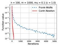
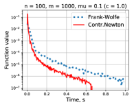
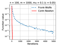
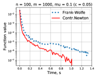
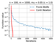
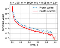
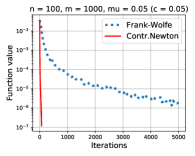
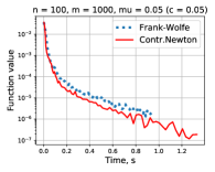
Figure 1: $n=100,\;m=1000$.

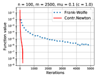
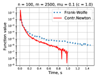
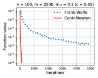
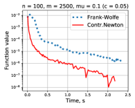
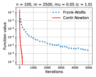
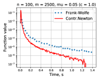
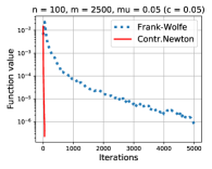
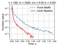
Figure 2: $n=100,\;m=2500$.

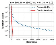
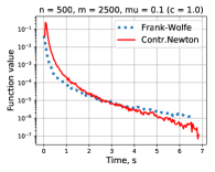
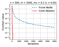
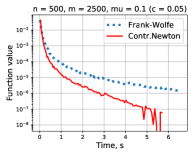
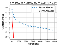
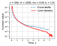
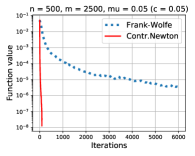
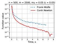
Figure 3: $n=500,\;m=2500$.

7 Discussion

In this paper, we present a new general framework of Contracting-Point methods, which can be used for developing affine-invariant optimization algorithms of different order. For the methods of order $p\geq 1$, we prove the following global convergence rate:

$$\begin{array}[]{rcl}F(x_{k})-F^{*}&\leq&{\cal O}\bigl{(}1/k^{p}\bigr{)},\quad k\geq 1.\end{array}$$

This is the same rate, as that of the basic high-order Proximal-Point scheme [22]. However, the methods from our paper are free from using the norms or any other characteristic parameters of the problem. This nice property makes Contracting-Point methods favourable for solving optimization problems over the sets with a non-Euclidean geometry (e.g. over the simplex or over a general convex polytope).

At the same time, it is known that in Euclidean case, the prox-type methods can be accelerated, achieving ${\cal O}(1/k^{p+1})$ global rate of convergence [2, 21, 6, 22]. Using additional one-dimensional search at each iteration, this rate can be improved up to ${\cal O}(1/k^{\frac{3p+1}{2}})$ (see [11, 22]). The latter rate is shown to be optimal [1, 20]. To the best of our knowledge, the lower bounds for high-order methods in general non-Euclidean case remain unknown. However, the worst-case oracle complexity of the classical Frank-Wolfe algorithm (the case $p=1$ in our framework) is proven to be near-optimal for smooth minimization over $\|\cdot\|_{\infty}$-balls [13].

Another open question is a possibility of efficient implementation of our methods for the case $p\geq 3$. In view of absence of explicit regularizer (contrary to the prox-type methods), the subproblem in (20) can be nonconvex. Hence, it seems hard to find its global minimizer. We hope that for some problem classes, it is still feasible to satisfy the inexact stationarity condition (23) by reasonable amount of computations. We keep this question for further investigation.

Appendix

In this section, we state some simple facts about maximization of multilinear symmetric forms. For a fixed $p\geq 1$, let us consider $(p+1)$-linear symmetric form $A$. For a set of vectors $h_{1},\dots,h_{p+1}\in\mathbb{E}$, we have

$$\begin{array}[]{rcl}A[h_{1},\dots,h_{p+1}]&\in&\mathbb{R}.\end{array}$$

For two vectors $u,v\in\mathbb{E}$ and integers $i,j\geq 0$ such that $i+j=p+1$, we use the following shorter notation:

$$\begin{array}[]{rcl}A[u]^{i}[v]^{j}&\stackrel{{\scriptstyle\mathrm{def}}}{{=}}&A[\underbrace{u,\dots,u}_{i\;\text{times}},\underbrace{v,\dots,v}_{j\;\text{times}}].\end{array}$$

Let us fix arbitrary compact convex set $S\subset\mathbb{E}$. We are interested to bound the variation of $A$ over two vectors from $S$, by that over the only one vector:

$$\begin{array}[]{rcl}\sup\limits_{u,v\in S}|A[u]^{p}[v]|&\leq&{\mathcal{C}}_{p}\sup\limits_{h\in S}|A[h]^{p+1}|,\end{array}$$ (34)

for some constant ${\mathcal{C}}_{p}$. Note, that if $S$ is a ball in the Euclidean norm, then ${\mathcal{C}}_{p}=1$, and the values of both supremums are equal (see Appendix 1 in [24], and Section 2.3 in [17]). In what follows, our aim is to estimate the value of ${\mathcal{C}}_{p}$ for arbitrary $S$. Namely, we establish the following bound.

Proposition 1

For any compact convex set $S$, (34) holds with

$$\begin{array}[]{rcl}{\mathcal{C}}_{p}&=&\frac{(p+1)^{p+1}+p^{p+1}+1}{(p+1)!}\;\;\leq\;\;\frac{2(p+1)^{p}}{p!}.\end{array}$$ (35)

Proof:

For a pair of integers $n,k\geq 0$, let us denote by $\binom{n}{k}$ the binomial coefficients, given by the formula

$$\begin{array}[]{rcl}\binom{n}{k}&\stackrel{{\scriptstyle\mathrm{def}}}{{=}}&\frac{n(n-1)\cdots(n-k+1)}{k!},\end{array}$$

and by ${n\brace k}$ we denote the Stirling numbers of the second kind. By definition, ${n\brace k}$ is equal to the number of ways to partition a set of $n$ objects into $k$ nonempty subsets. The following important identity holds (see, for example, [12]):

$$\begin{array}[]{rcl}k^{n}&=&k!\sum\limits_{r=1}^{k}\frac{{n\brace r}}{(k-r)!},\qquad n\geq 1.\end{array}$$ (36)

Note also, that ${n\brace n}=1$, and ${n\brace k}=0$, for $k>n$.

Now, let us fix arbitrary vectors $u,v\in S$, and consider the set of their convex combinations $h_{i}=\alpha_{i}u+(1-\alpha_{i})v\in S$ for some $\alpha_{i}\in(0,1)$, $1\leq i\leq p$. The binomial theorem yields the system of equations

$$\begin{array}[]{rcl}A[h_{i}]^{p+1}&=&\sum\limits_{j=0}^{p+1}\binom{p+1}{j}\alpha_{i}^{j}(1-\alpha_{i})^{p+1-j}A[u]^{j}[v]^{p+1-j},\qquad 1\leq i\leq p.\end{array}$$ (37)

For the choice $\alpha_{i}=\frac{i}{i+1}$, we have $1-\alpha_{i}=\frac{1}{i+1}$, and

$$\begin{array}[]{rcl}\alpha_{i}^{j}(1-\alpha_{i})^{p+1-j}&=&\frac{i^{j}}{(i+1)^{p+1}}.\end{array}$$

Therefore, introducing a vector $x\in\mathbb{R}^{p}$,

$$\begin{array}[]{rcl}x^{(j)}&\equiv&\binom{p+1}{j}A[u]^{j}[v]^{p+1-j},\qquad 1\leq j\leq p,\end{array}$$

from (37) we obtain the linear system $\boxed{Bx=c}$ with matrix

$$\begin{array}[]{rcl}B^{(i,j)}&\equiv&i^{j},\qquad 1\leq i,j\leq p,\end{array}$$ (38)

and the right hand side vector

$$\begin{array}[]{rcl}c^{(i)}&\equiv&(i+1)^{p+1}\bigl{(}A[h_{i}]^{p+1}-(1-\alpha_{i})^{p+1}A[v]^{p+1}-\alpha_{i}^{p+1}A[u]^{p+1}\bigr{)},\qquad 1\leq i\leq p.\end{array}$$ (39)

The matrix given by (38) looks as follows

$$\begin{array}[]{rcl}B&=&\begin{pmatrix}&1&1&1&\dots&1\\ &2&2^{2}&2^{3}&\dots&2^{p}\\ &3&3^{2}&3^{3}&\dots&3^{p}\\ &\vdots&\vdots&\vdots&\ddots&\vdots\\ &p&p^{2}&p^{3}&\dots&p^{p}\end{pmatrix}.\end{array}$$

This structure is similar to that one of the Vandermonde matrix. By the Gaussian elimination process we can build a sequence of matrices

$$\begin{array}[]{rcl}B&=&B_{1}\;\;\mapsto\;\;B_{2}\;\;\mapsto\;\;\dots\;\;\mapsto\;\;B_{p},\end{array}$$

such that $B_{p}$ is upper triangular, and the corresponding sequence of the right hand side vectors

$$\begin{array}[]{rcl}c&=&c_{1}\;\;\mapsto\;\;c_{2}\;\;\mapsto\;\;\dots\;\;\mapsto\;\;c_{p},\end{array}$$

having the same solution $x$ as the initial system:

$$\begin{array}[]{rcl}B_{t}x=c_{t},\qquad 1\leq t\leq p.\end{array}$$

Then, the last component of the solution can be easily found:

$$\begin{array}[]{rcl}(p+1)A[u]^{p}[v]&=&x^{(p)}\;\;=\;\;\frac{c_{p}^{(p)}}{B_{p}^{(p,p)}},\end{array}$$ (40)

from which we may obtain the required bound for the left hand side of (34). Thus, we are interested to investigate the elements of $B_{p}$ and $c_{p}$.

Let us prove by induction, that for every $1\leq t\leq p$, it holds

$$\begin{array}[]{rcl}B_{t}^{(i,j)}&=&\begin{cases}i!{j\brace i}&\text{if}\;i\leq t;\\ i!\sum\limits_{r=t}^{i}\frac{{j\brace r}}{(i-r)!}&\text{otherwise}.\end{cases}\end{array}$$ (41)

For $t=1$, (41) follows from (36), and this is the base of the induction. At step $t$ of the Gaussian elimination, we have the matrix $B_{t}$. First, we freeze its $t$-th row for all the following matrices:

$$\begin{array}[]{rcl}B_{t}^{(t,j)}&=&B_{t+1}^{(t,j)}\;\;=\;\;B_{t+2}^{(t,j)}\;\;=\;\;\dots\;\;=\;\;B_{p}^{(t,j)}\;\;=\;\;t!{j\brace t},\qquad 1\leq j\leq p.\end{array}$$

Then, we subtract this row from all the rows located below, scaled by an appropriate factor, for $t<i\leq p$:

$$\begin{array}[]{rcl}B_{t+1}^{(i,j)}&=&B_{t}^{(i,j)}-\frac{B_{t}^{(i,t)}}{B_{t}^{(t,t)}}\cdot B_{t}^{(t,j)},\qquad 1\leq j\leq p.\end{array}$$

Note, that $B_{t}^{(t,t)}=t!$ and $B_{t}^{(i,t)}=\frac{i!}{(i-t)!}$. Therefore, we obtain

$$\begin{array}[]{rcl}B_{t+1}^{(i,j)}&=&i!\sum\limits_{r=t}^{i}\frac{{j\brace r}}{(i-r)!}\;\;-\;\;\frac{i!{j\brace t}}{(i-t)!}\;\;=\;\;i!\sum\limits_{r=t+1}^{i}\frac{{j\brace r}}{(i-r)!},\qquad 1\leq j\leq p,\end{array}$$

and this is (41) for the next step. Hence (41) is established by induction for all $1\leq t\leq p$.

Similarly, we have the update rules for the right hand sides:

$$\begin{array}[]{rcl}c_{t}^{(t)}&=&c_{t+1}^{(t)}\;\;=\;\;\dots\;\;=\;\;c_{p}^{(t)},\end{array}$$

and for $t<i\leq p$:

$$\begin{array}[]{rcl}c_{t+1}^{(i)}&=&c_{t}^{(i)}-\frac{B_{t}^{(i,t)}}{B_{t}^{t,t}}c_{t}^{(t)}\;\;=\;\;c_{t}^{(i)}-\binom{i}{t}c_{t}^{(t)}\\ \\ &=&c_{t-1}^{(i)}-\binom{i}{t-1}c_{t-1}^{(t-1)}-\binom{i}{t}c_{t}^{(t)}\;\;=\dots\\ \\ &=&c_{1}^{(i)}-\sum\limits_{r=1}^{t}\binom{i}{r}c_{r}^{(r)}.\end{array}$$

Therefore, for the resulting vector $c_{p}$ we have a recurrence:

$$\begin{array}[]{rcl}c_{p}^{(i)}=c_{1}^{(i)}-\sum\limits_{r=1}^{i-1}\binom{i}{r}c_{p}^{(r)},\qquad 1\leq i\leq p.\end{array}$$ (42)

From (42) we obtain an explicit expression for $c_{p}$ using only the initial values:

$$\begin{array}[]{rcl}c_{p}^{(i)}&=&\sum\limits_{j=1}^{i}(-1)^{i-j}\binom{i}{j}c^{(j)}_{1},\qquad 1\leq i\leq p.\end{array}$$ (43)

Indeed, for $i=1$ (43) follows directly from (42). Assume by induction that (43) holds for all $1\leq i\leq n$, for some $n$. Then, for the next index we have

$$\begin{array}[]{rcl}c_{p}^{(n+1)}&\stackrel{{\scriptstyle(\ref{CRecurr})}}{{=}}&c_{1}^{(n+1)}-\sum\limits_{r=1}^{n}\binom{n+1}{r}c_{p}^{(r)}\\ \\ &\stackrel{{\scriptstyle(\ref{CExplicit})}}{{=}}&c_{1}^{(n+1)}-\sum\limits_{r=1}^{n}\sum\limits_{j=1}^{r}(-1)^{r-j}\binom{n+1}{r}\binom{r}{j}c_{1}^{(j)}\\ \\ &=&c_{1}^{(n+1)}-\sum\limits_{j=1}^{n}\biggl{(}\sum\limits_{r=j}^{n}(-1)^{r-j}\binom{n+1}{r}\binom{r}{j}\biggr{)}c_{1}^{(j)}\\ \\ &=&c_{1}^{(n+1)}+\sum\limits_{j=1}^{n}(-1)^{n+1-j}\binom{n+1}{j}c_{1}^{(j)},\end{array}$$

where the last equation follows from simple observations:

$$\begin{array}[]{rcl}\sum\limits_{r=j}^{n}(-1)^{r-j}\binom{n+1}{r}\binom{r}{j}&=&\sum\limits_{r=j}^{n}(-1)^{r-j}\frac{(n+1)!\,r!}{r!\,(n+1-r)!\,j!\,(r-j)!}\\ \\ &=&\binom{n+1}{j}\sum\limits_{r=j}^{n}(-1)^{r-j}\binom{n+1-j}{r-j}\\ \\ &=&\binom{n+1}{j}\sum\limits_{l=0}^{n-j}(-1)^{l}\binom{n+1-j}{l}\\ \\ &=&\binom{n+1}{j}\Bigl{(}(1-1)^{n+1-j}-(-1)^{n+1-j}\Bigr{)}\;\;=\;\;(-1)^{n-j}\binom{n+1}{j}.\end{array}$$

Hence (43) is established by induction for all $1\leq i\leq p$.

Let us denote by ${\mathcal{V}}$ the supremum from the right hand side of (34):

$$\begin{array}[]{rcl}\mathcal{V}&\stackrel{{\scriptstyle\mathrm{def}}}{{=}}&\sup\limits_{h\in S}|A[h]^{p+1}|.\end{array}$$

Then, in view of (39), we have

$$\begin{array}[]{rcl}|c_{1}^{(j)}|&=&|c^{(j)}|\;\;\leq\;\;((p+1)^{p+1}+p^{p+1}+1)\mathcal{V},\qquad 1\leq j\leq p,\end{array}$$ (44)

and, consequently

$$\begin{array}[]{rcl}|A[u]^{p}[v]|&\overset{\eqref{AuvEqual},\eqref{PolySystemGauss}}{=}&\frac{|c_{p}^{(p)}|}{(p+1)!}\;\;\overset{\eqref{CExplicit}}{=}\;\;\frac{1}{(p+1)!}\Big{|}\sum\limits_{j=1}^{p}(-1)^{p-j}\binom{p}{j}c_{1}^{(j)}\Big{|}\\ \\ &\overset{\eqref{C1Bound}}{\leq}&\frac{((p+1)^{p+1}+p^{p+1}+1){\mathcal{V}}}{(p+1)!}\Big{|}\sum\limits_{j=1}^{p}(-1)^{p-j}\binom{p}{j}\Big{|}\;\;=\;\;\mathcal{C}_{p}\mathcal{V}.\end{array}$$

Since $u,v\in S$ are arbitrary vectors, we have (35) established. $\Box$

Let us consider the most important cases, when $p=1$ and $p=2$.

Corollary 1

For any symmetric bilinear form $A:\mathbb{E}\times\mathbb{E}\to\mathbb{R}$ and any compact convex set $S\subset\mathbb{E}$, it holds

$$\begin{array}[]{rcl}\sup\limits_{u,v\in S}|A[u,v]|&\leq&3\sup\limits_{h\in S}|A[h,h]|.\end{array}$$ (45)

Corollary 2

For any symmetric trilinear form $A:\mathbb{E}\times\mathbb{E}\times\mathbb{E}\to\mathbb{R}$ and any compact convex set $S\subset\mathbb{E}$, it holds

$$\begin{array}[]{rcl}\sup\limits_{u,v\in S}|A[u,u,v]|&\leq&6\sup\limits_{h\in S}|A[h,h,h]|.\end{array}$$ (46)

It appears that the bound in (45) is tight.

Example 4

Consider the following symmetric bilinear form on two-dimensional space $\mathbb{E}=\mathbb{R}^{2}$:

$$\begin{array}[]{rcl}A[u,v]&=&u^{(1)}v^{(1)}-2u^{(2)}v^{(2)},\qquad u,v\in\mathbb{R}^{2},\end{array}$$

and let

$$\begin{array}[]{rcl}S&=&\bigl{\{}x\in\mathbb{R}^{2}\;:\;x^{(1)}=1,\;x^{(2)}\in[-1,1]\bigr{\}}.\end{array}$$

Then,

$$\begin{array}[]{rcl}\sup\limits_{u,v\in S}|A[u,v]|&=&\sup\limits_{\alpha,\beta\in[-1,1]}|1-2\alpha\beta|\;\;=\;\;3.\end{array}$$

However,

$$\begin{array}[]{rcl}\sup\limits_{h\in S}|A[h,h]|&=&\sup\limits_{\alpha\in[0,1]}|1-2\alpha|\;\;=\;\;1.\end{array}$$

If it happens that our bilinear form is positive semidefinite (e.g. it is determined by the Hessian of a convex function), the constant in (45) can be improved to be $1$, so the both supremums are equal.

Proposition 2

Let symmetric bilinear form $A:\mathbb{E}\times\mathbb{E}\to\mathbb{R}$ be positive semidefinite:

$$\begin{array}[]{rcl}A[h,h]&\geq&0,\qquad h\in\mathbb{E}.\end{array}$$

Then, for any set $S\subset\mathbb{E}$, it holds

$$\begin{array}[]{rcl}\sup\limits_{u,v\in S}|A[u,v]|&=&\sup\limits_{h\in S}A[h,h].\end{array}$$

Proof:

Indeed, by the Eigenvalue Decomposition, for some $r\geq 0$, there exists a set of linear forms $a_{1},\dots,a_{r}\in\mathbb{E}^{*}$ and positive numbers $\lambda_{1},\dots,\lambda_{r}>0$ such that

$$\begin{array}[]{rcl}A[u,v]&=&\sum\limits_{i=1}^{r}\lambda_{i}\langle a_{i},u\rangle\langle a_{i},v\rangle,\qquad u,v\in S.\end{array}$$

Therefore, using Cauchy-Bunyakovsky-Schwarz inequality, we get

$$\begin{array}[]{rcl}|A[u,v]|&\leq&\Bigl{(}\sum\limits_{i=1}^{r}\lambda_{i}\langle a_{i},u\rangle^{2}\Bigr{)}^{1/2}\Bigl{(}\sum\limits_{i=1}^{r}\lambda_{i}\langle a_{i},v\rangle^{2}\Bigr{)}^{1/2}\\ \\ &=&\bigl{(}A[u,u]\bigr{)}^{1/2}\bigl{(}A[v,v]\bigr{)}^{1/2}\\ \\ &\leq&\sup\limits_{h\in S}A[h,h].\end{array}$$

$\Box$

References

• [1] Yossi Arjevani, Ohad Shamir, and Ron Shiff. Oracle complexity of second-order methods for smooth convex optimization. Mathematical Programming, 178(1-2):327–360, 2019.
• [2] Michel Baes. Estimate sequence methods: extensions and approximations. Institute for Operations Research, ETH, Zürich, Switzerland, 2009.
• [3] Heinz H Bauschke, Jérôme Bolte, and Marc Teboulle. A descent lemma beyond lipschitz gradient continuity: first-order methods revisited and applications. Mathematics of Operations Research, 42(2):330–348, 2016.
• [4] Coralia Cartis and Katya Scheinberg. Global convergence rate analysis of unconstrained optimization methods based on probabilistic models. Mathematical Programming, 169(2):337–375, 2018.
• [5] Andrew R Conn, Nicholas IM Gould, and Philippe L Toint. Trust region methods. SIAM, 2000.
• [6] Nikita Doikov and Yurii Nesterov. Contracting proximal methods for smooth convex optimization. CORE Discussion Papers 2019/27, 2019.
• [7] Nikita Doikov and Yurii Nesterov. Minimizing uniformly convex functions by cubic regularization of Newton method. arXiv preprint arXiv:1905.02671, 2019.
• [8] Nikita Doikov and Yurii Nesterov. Convex optimization based on global lower second-order models. arXiv preprint arXiv:2006.08518, 2020.
• [9] Nikita Doikov and Yurii Nesterov. Inexact tensor methods with dynamic accuracies. arXiv preprint arXiv:2002.09403, 2020.
• [10] Marguerite Frank and Philip Wolfe. An algorithm for quadratic programming. Naval research logistics quarterly, 3(1-2):95–110, 1956.
• [11] Alexander Gasnikov, Pavel Dvurechensky, Eduard Gorbunov, Evgeniya Vorontsova, Daniil Selikhanovych, César A Uribe, Bo Jiang, Haoyue Wang, Shuzhong Zhang, Sébastien Bubeck, Jiang Qijia, Yin Tat Lee, Li Yuanzhi, and Sidford Aaron. Near optimal methods for minimizing convex functions with Lipschitz $p$-th derivatives. In Conference on Learning Theory, pages 1392–1393, 2019.
• [12] Ronald L Graham, Donald E Knuth, Oren Patashnik, and Stanley Liu. Concrete mathematics: a foundation for computer science. Computers in Physics, 3(5):106–107, 1989.
• [13] Cristóbal Guzmán and Arkadi Nemirovski. On lower complexity bounds for large-scale smooth convex optimization. Journal of Complexity, 31(1):1–14, 2015.
• [14] Martin Jaggi. Revisiting Frank-Wolfe: Projection-free sparse convex optimization. In International Conference on Machine Learning, pages 427–435, 2013.
• [15] Dmitry Kamzolov, Alexander Gasnikov, and Pavel Dvurechensky. On the optimal combination of tensor optimization methods. arXiv preprint arXiv:2002.01004, 2020.
• [16] Haihao Lu, Robert M Freund, and Yurii Nesterov. Relatively smooth convex optimization by first-order methods, and applications. SIAM Journal on Optimization, 28(1):333–354, 2018.
• [17] Arkadi Nemirovski. Interior point polynomial time methods in convex programming. Lecture notes, 2004.
• [18] Yurii Nesterov. Gradient methods for minimizing composite functions. Mathematical Programming, 140(1):125–161, 2013.
• [19] Yurii Nesterov. Complexity bounds for primal-dual methods minimizing the model of objective function. Mathematical Programming, 171(1-2):311–330, 2018.
• [20] Yurii Nesterov. Lectures on convex optimization, volume 137. Springer, 2018.
• [21] Yurii Nesterov. Implementable tensor methods in unconstrained convex optimization. Mathematical Programming, pages 1–27, 2019.
• [22] Yurii Nesterov. Inexact accelerated high-order proximal-point methods. CORE Discussion Papers 2020/8, 2020.
• [23] Yurii Nesterov. Superfast second-order methods for unconstrained convex optimization. CORE Discussion Papers 2020/7, 2020.
• [24] Yurii Nesterov and Arkadii Nemirovskii. Interior-point polynomial algorithms in convex programming. SIAM, 1994.