Large Deviations Approach to Random Recurrent Neuronal Networks:
Parameter Inference and Fluctuation–Induced Transitions

Abstract

We here unify the field theoretical approach to neuronal networks with large deviations theory. For a prototypical random recurrent network model with continuous-valued units, we show that the effective action is identical to the rate function and derive the latter using field theory. This rate function takes the form of a Kullback-Leibler divergence which enables data-driven inference of model parameters and calculation of fluctuations beyond mean–field theory. Lastly, we expose a regime with fluctuation–induced transitions between mean–field solutions.

Introduction.–

Biological neuronal networks are systems with many degrees of freedom and intriguing properties: their units are coupled in a directed, non-symmetric manner, so that they typically operate outside thermodynamic equilibrium [1, 2]. The primary analytical method to study neuronal networks has been mean-field theory [3, 4, 5, 6, 7, 8]. Its field-theoretical basis has been exposed only recently [9, 10]. However, to understand the parallel and distributed information processing performed by neuronal networks, the study of the forward problem – from the microscopic parameters of the model to its dynamics – is not sufficient. One additionally faces the inverse problem of determining the parameters of the model given a desired dynamics and thus function. Formally, one needs to link statistical physics with concepts from information theory and statistical inference.

We here expose a tight relation between statistical field theory of neuronal networks, large deviations theory, information theory, and inference. To this end, we generalize the probabilistic view of large deviations theory, which yields rigorous results for the leading order behavior in the network size $N$ [11, 12], to arbitrary single unit dynamics, transfer functions, and multiple populations. We furthermore show that the central quantity of large deviations theory, the rate function, is identical to the effective action in statistical field theory. This link exposes a second relation: Bayesian inference and prediction are naturally formulated within this framework, spanning the arc to information processing. Concretely, we develop a method for parameter inference from transient data for single- and multi-population networks. Lastly, we overcome the inherent limit of mean-field theory—its neglect of fluctuations. We develop a theory for fluctuations of the order parameter when the intrinsic timescale is large and discover a regime with fluctuation–induced transitions between two coexisting mean–field solutions.

First, we introduce the model in its most general form. Then, we develop the theory for a single population. Last, we generalize it to multiple populations.

Model.-

We consider block-structured random networks of $N=\sum_{\alpha}N_{\alpha}$ nonlinearly interacting units $x_{i}^{\alpha}(t)$ driven by an external input $\xi_{i}^{\alpha}(t)$. The dynamics of the $i$-th unit in the $\alpha$-th population is governed by the stochastic differential equation

$$\tau_{\alpha}\dot{x}_{i}^{\alpha}(t) =-U_{\alpha}^{\prime}(x_{i}^{\alpha}(t))+\sum_{\beta}\sum_{j=1}^{N_{\beta}}J_{ij}^{\alpha\beta}\phi(x_{j}^{\beta}(t))+\xi_{i}^{\alpha}(t).$$ (1)

In the absence of recurrent and external inputs, the units undergo an overdamped motion with time constant $\tau_{\alpha}$ in a potential $U_{\alpha}(x)$. The $J_{ij}^{\alpha\beta}$ are independent and identically Gaussian-distributed random coupling weights with zero mean and population-specific variance $\langle(J_{ij}^{\alpha\beta})^{2}\rangle=g_{\alpha\beta}^{2}/N_{\beta}$ where the coupling strength $g_{\alpha\beta}$ controls the heterogeneity of the weights. The time-varying external inputs $\xi_{i}^{\alpha}(t)$ are independent Gaussian white-noise processes with zero mean and correlation functions $\left\langle\xi_{i}^{\alpha}(t_{1})\xi_{j}^{\beta}(t_{2})\right\rangle=2D_{\alpha}\delta_{ij}\delta_{\alpha\beta}\delta(t_{1}-t_{2})$. The single-population model corresponds to the one studied in Ref. [4] if the external input vanishes, $D=0$, the potential is quadratic, $U(x)=\frac{1}{2}x^{2}$, and the transfer function is sigmoidal, $\phi(x)=\tanh(x)$; for $D=\frac{1}{2}$, $U(x)=-\log(A^{2}-x^{2})$, and $\phi(x)=x$ it corresponds to the one in Ref. [11], which is inspired by the dynamical spin glass model of Ref. [13].

Field theory.-

The field-theoretical treatment of Eq. (1) employs the Martin–Siggia–Rose–de Dominicis–Janssen path integral formalism [14, 15, 16, 17]. We denote the expectation over paths across different realizations of the noise $\xi$ as (Appendix A1)

$$\left\langle\cdot\right\rangle_{\bm{x}|\bm{J}} \equiv\left\langle\left\langle\cdot\right\rangle_{\bm{x}|\bm{J},\bm{\xi}}\right\rangle_{\bm{\xi}}=\int\mathcal{D}\bm{x}\,\int\mathcal{D}\bm{\tilde{x}}\,\cdot\,e^{S_{0}(\bm{x},\bm{\tilde{x}})-\bm{\tilde{x}}^{\!\mathsf{T}}\bm{J}\phi(\bm{x})},$$

where $\left\langle\cdot\right\rangle_{\bm{x}|\bm{J},\bm{\xi}}$ integrates over the unique solution of Eq. (1) given one realization $\bm{\xi}$ of the noise. Here, $S_{0}(\bm{x},\bm{\tilde{x}})=\bm{\tilde{x}}^{\!\mathsf{T}}(\dot{\bm{x}}+U^{\prime}(\bm{x}))+D\bm{\tilde{x}}^{\!\mathsf{T}}\bm{\tilde{x}}$ is the action of the uncoupled neurons. We use the shorthand notation $\bm{a}^{\!\mathsf{T}}\bm{b}=\sum_{i=1}^{N}\int_{0}^{T}\mathrm{d}t\,a_{i}(t)b_{i}(t)$.

For large $N$, the system becomes self-averaging, a property known from many disordered systems with large numbers of degrees of freedom: the collective behavior is stereotypical, independent of the realization $J_{ij}$. A self–averaging observable has a sharply peaked distribution over realizations of $\bm{J}$—the observable always attains the same value, close to its average. This, however, only holds for observables averaged over all units, reminiscent of the central limit theorem. These are generally of the form $\sum_{i=1}^{N}\ell(x_{i})$, where $\ell$ is an arbitrary functional of a single unit’s trajectory. It is therefore convenient to introduce the scaled cumulant–generating functional

$$W_{N}(\ell) :=\frac{1}{N}\ln\left\langle\left\langle e^{\sum_{i=1}^{N}\ell(x_{i})}\right\rangle_{\bm{x}|\bm{J}}\right\rangle_{\bm{J}},$$ (2)

where the prefactor $1/N$ makes sure that $W_{N}$ is an intensive quantity, reminiscent of the bulk free energy [18]. In fact, we will show that the $N$-dependence vanishes in the limit $N\to\infty$ because the system decouples.

Performing the average over $\bm{J}$, i.e. evaluating $\langle e^{-\bm{\tilde{x}}^{\!\mathsf{T}}\bm{J}\phi(\bm{x})}\rangle_{\bm{J}}$, and introducing the auxiliary field

$$C(t_{1},t_{2}) :=\frac{1}{N}\sum_{i=1}^{N}\phi(x_{i}(t_{1}))\,\phi(x_{i}(t_{2}))$$ (3)

as well as the conjugate field $\tilde{C}$, we can write $W_{N}$ as (Appendix A1)

$$W_{N}(\ell) =\frac{1}{N}\ln\,\int\mathcal{D}C\,\int\mathcal{D}\tilde{C}\,e^{-N\,C^{\!\mathsf{T}}\tilde{C}+N\,\Omega_{\ell}(C,\tilde{C})},$$ (4)

$$\Omega_{\ell}(C,\tilde{C}) :=\ln\,\int\mathcal{D}x\,\int\mathcal{D}\tilde{x}\,e^{S_{0}(x,\tilde{x})+\frac{g^{2}}{2}\tilde{x}^{\!\mathsf{T}}C\tilde{x}+\phi^{\!\mathsf{T}}\tilde{C}\phi+\ell(x)}.$$

The effective action is defined as the Legendre transform of $W_{N}(\ell)$,

$$\Gamma_{N}(\mu) :=\int\mathcal{D}x\,\mu(x)\,\ell_{\mu}(x)-W_{N}(\ell_{\mu}),$$ (5)

where $\ell_{\mu}$ is determined implicitly by the condition $\mu=W_{N}^{\prime}(\ell_{\mu})$ and the derivative $W_{N}^{\prime}(\ell)$ has to be understood as a generalized derivative, the coefficient of the linearization akin to a Fréchet derivative [19].

Note that $W_{N}$ and $\Gamma_{N}$ are, respectively, generalizations of a cumulant–generating functional and of the effective action [20] because both map a functional ($\ell$ or $\mu$) to the reals. For the choice $\ell(x)=j^{\!\mathsf{T}}x$, where $j(t)$ is an arbitrary function, we recover the usual cumulant–generating functional of the single unit’s trajectory (Appendix A4) and the corresponding effective action.

Rate function.-

Any network–averaged observable, for which we may expect self-averaging to hold, can likewise be obtained from the empirical measure

$$\mu(y) :=\frac{1}{N}\sum_{i=1}^{N}\delta(x_{i}-y),$$ (6)

since $\frac{1}{N}\sum_{i=1}^{N}\ell(x_{i})=\int\mathcal{D}y\,\mu(y)\ell(y)$. Of particular interest is the leading–order exponential behavior of the distribution of empirical measures $P(\mu)=\langle\langle P(\mu\,|\,\bm{x})\rangle_{\bm{x}|\bm{J}}\rangle_{\bm{J}}$ across realizations of $\bm{J}$ and $\bm{\xi}$. This behavior in the large $N$ limit is described by what is known as the rate function

$$H(\mu) :=-\lim_{N\to\infty}\frac{1}{N}\ln P(\mu)$$ (7)

in large deviations theory [see e.g. 21]; $H(\mu)$ captures the leading exponential probability $P(\mu)\stackrel{{\scriptstyle N\gg 1}}{{\simeq}}e^{-N\,H(\mu)}$. For large $N$, the probability of an empirical measure that does not correspond to the minimum $H^{\prime}(\bar{\mu})=0$ is thus exponentially suppressed. Put differently, the system is self–averaging and the statistics of any network–averaged observable can be obtained using $\bar{\mu}$.

Similar as in field theory, it is convenient to introduce the scaled cumulant–generating functional of the empirical measure. Because $\frac{1}{N}\sum_{i=1}^{N}\ell(x_{i})=\int\mathcal{D}y\,\mu(y)\ell(y)$ holds for an arbitrary functional $\ell(x_{i})$ of the single unit’s trajectory $x_{i}$, Eq. (2) has the form of the scaled cumulant–generating functional for $\mu$ at finite $N$.

Using a saddle-point approximation for the integrals over $C$ and $\tilde{C}$ in Eq. (4) (Appendix A1), we get

$$W_{\infty}(\ell) =-C_{\ell}^{\!\mathsf{T}}\tilde{C}_{\ell}+\Omega_{\ell}(C_{\ell},\tilde{C}_{\ell}).$$ (8)

Both $C_{\ell}$ and $\tilde{C}_{\ell}$ are determined self-consistently by the saddle-point equations $C_{\ell}=\left.\partial_{\tilde{C}}\Omega_{\ell}(C,\tilde{C})\right|_{C_{\ell},\tilde{C}_{\ell}}$ and $\tilde{C}_{\ell}=\left.\partial_{C}\Omega_{\ell}(C,\tilde{C})\right|_{C_{\ell},\tilde{C}_{\ell}}$ where $\partial_{C}$ denotes a partial functional derivative.

From the scaled cumulant–generating functional, Eq. (8), we obtain the rate function via a Legendre transformation [22]: $H(\mu)=\int\mathcal{D}x\,\mu(x)\ell_{\mu}(x)-W_{\infty}(\ell)$ with $\ell_{\mu}$ implicitly defined by $\mu=W_{\infty}^{\prime}(\ell_{\mu})$. Note that $H(\mu)$ is still convex even if $\mu$ itself is multimodal. Comparing with Eq. (5), we observe that the rate function is equivalent to the effective action: $H(\mu)=\lim_{N\to\infty}\Gamma_{N}(\mu)$. The equation $\mu=W_{\infty}^{\prime}(\ell_{\mu})$ can be solved for $\ell_{\mu}$ to obtain a closed expression for the rate function viz. effective action (Appendix A2), one main result of our work,

$$H(\mu) =\int\mathcal{D}x\,\mu(x)\ln\frac{\mu(x)}{\left\langle\delta(\dot{x}+U^{\prime}(x)-\eta)\right\rangle_{\eta}},$$ (9)

where $\eta$ is a zero–mean Gaussian process with a correlation function that is determined by $\mu(x)$,

$$C_{\eta}(t_{1},t_{2})= 2D\,\delta(t_{1}-t_{2})$$

$$+g^{2}\negthinspace\int\mathcal{D}x\,\mu(x)\,\phi(x(t_{1}))\phi(x(t_{2})).$$ (10)

For $D=\frac{1}{2}$, $U(x)=-\log(A^{2}-x^{2})$, and $\phi(x)=x$, Eq. (9) can be shown to be a equivalent to the mathematically rigorous result obtained in the seminal work by Ben Arous and Guionnet (Appendix A3).

The rate function Eq. (9) takes the form of a Kullback-Leibler divergence. Thus, it possesses a minimum at

$$\bar{\mu}(x) =\left\langle\delta(\dot{x}+U^{\prime}(x)-\eta)\right\rangle_{\eta}.$$ (11)

This most likely measure corresponds to the well-known self-consistent stochastic dynamics that is obtained in field theory [4, 9, 10, 23]. Note that the correlation function of the effective stochastic input $\eta$ at the minimum depends self-consistently on $\bar{\mu}(x)$ through Eq. (10). However, the rate function $H(\mu)$ contains more information. It quantifies the suppression of departures $\mu-\bar{\mu}$ from the most likely measure and therefore allows the assessment of fluctuations that are beyond the scope of the classical mean-field result.

Parameter Inference.–

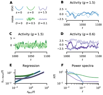
Figure 1: Maximum likelihood parameter estimation for $\phi(x)=\mathrm{erf}(\sqrt{\pi}x/2)$, potential $U(x)=\frac{1}{2}x^{2}+s\ln\cosh x$, and external noise $D$. A Color–coded sketch of potential and noise. B-D Activity of three randomly chosen units for coupling strengths $g$ indicated in title. E Parameter estimation via non-negative least squares regression (black lines) based on Eq. (12). F Power spectra on the left– (dark, solid curves) and right–hand–sides (light, dotted curves) of Eq. (12) for the inferred parameters. Further parameters: $N=10,000$, temporal discretization $dt=10^{-2}$, simulation time $T=1,000$, time-span discarded to reach steady state $T_{0}=100$.

The rate function opens the way to address the inverse problem: given the network–averaged activity statistics, encoded in the corresponding empirical measure $\mu$, what are the statistics of the connectivity and the external input, i.e. $g$ and $D$?

We determine the parameters using maximum likelihood estimation. Using Eq. (7) and Eq. (9), the likelihood of the parameters is given by

$$\ln P(\mu\,|\,g,D) \simeq-NH(\mu\,|\,g,D),$$

where $\simeq$ denotes equality in the limit $N\to\infty$ and we made the dependence on $g$ and $D$ explicit. The maximum likelihood estimate of the parameters $g$ and $D$ corresponds to the minimum of the Kullback–Leibler divergence $H$, Eq. (9), on the right hand side. Evaluating the derivative of $H(\mu\,|\,g,D)$ yields (Appendix B1)

$$\partial_{a}\ln P(\mu\,|\,g,D) \simeq-\frac{N}{2}\mathrm{tr}\left((C_{0}-C_{\eta})\frac{\partial C_{\eta}^{-1}}{\partial a}\right),$$

where we abbreviated $a\in\{g,D\}$ and defined $C_{0}(t_{1},t_{2})\equiv\int\mathcal{D}x\,\mu(x)\,\big{(}\dot{x}(t_{1})+U^{\prime}(x(t_{1}))\big{)}\,\big{(}\dot{x}(t_{2})+U^{\prime}(x(t_{2}))\big{)}$. The derivative vanishes for $C_{0}=C_{\eta}$. Assuming stationarity, in Fourier domain this condition reads

$$\mathcal{S}_{\dot{x}+U^{\prime}(x)}(f) =2D+g^{2}\mathcal{S}_{\phi(x)}(f),$$ (12)

where $\mathcal{S}_{X}(f)$ denotes the network–averaged power spectrum of the observable $X$. Using non–negative least squares [24], Eq. (12) allows a straightforward inference of $g$ and $D$ (Fig. 1). To determine the transfer function $\phi$ and the potential $U$, one can use model comparison techniques (Appendix B2). Using the inferred parameters, we can also predict the future activity of a unit from the knowledge of its recent past (Appendix B3).

Fluctuations.–

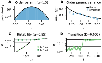
Figure 2: Order parameter fluctuations for $\phi(x)=\mathrm{erf}(\sqrt{\pi}x/2)$ (A,B) and meta-stability for $\phi(x)=\mathrm{clip}(\tan(x),-1,1)$ (C,D). A Temporal order parameter statistics across ten simulations (bars) and theory (solid curve) from Eq. (13). B Order parameter variance for $10$ realizations of the connectivity with standard error of the mean (symbols) and theory (solid curve) from Eq. (13). C Mean order parameter for different initial values $q_{0}$ from simulations (symbols) and self–consistent theory (solid curves). D Fluctuation induced bistability of the order parameter for $N=750$, $g=0.95$. $T=5,000$ in A,D; $U(x)=\frac{1}{2}x^{2}$; further parameters as in Fig. 1.

The rate function allows us to go beyond mean–field theory and examine fluctuations of the order parameter. Here, we use the network-averaged variance $q(t)=C(t,t)$ from Eq. (3) as an order parameter and restrict the discussion to the case $U(x)=\frac{1}{2}x^{2}.$

Fig. 2A shows the distribution of $q(t)$ across time and across realizations of the connectivity. The fluctuations across realizations of the connectivity can be computed from the curvature of the rate function $I(C)$ that is obtained from (9) by the contraction principle (Appendix C1). In a stationary state and considering only the fluctuations across realizations of the connectivity, for slow recurrent dynamics $\tau_{c}\gg 1$ we obtain the approximation for the fluctuations of $q$

$$\langle(q-\langle q\rangle_{\bm{J}})^{2}\rangle_{\bm{J}} =\frac{\langle(\phi\phi-\langle\phi\phi\rangle_{0})^{2}\rangle_{0}}{N\left(1-g^{2}\left(\langle\phi^{\prime\prime}\phi\rangle_{0}+\langle\phi^{\prime}\phi^{\prime}\rangle_{0}\right)\right)^{2}}.$$ (13)

Here, $\langle fg\rangle_{0}\equiv\langle f(x(t))g(x(t))\rangle_{0}$ denotes an expectation w.r.t. the self–consistent measure (11). For vanishing noise, $D=0$, and $g>1$, the dynamics are slow and the theory matches the empirical fluctuations very well (Fig. 2A,B). Deviations in Fig. 2B are caused by two effects: For $g\searrow 1$, periodic solutions appear as a finite-size effect; for growing $g$, the timescale $\tau_{c}$ decreases, eventually violating the assumption $\tau_{c}\gg 1$ entering Eq. (13). Rate functions like $I(C)$ in general also allow one to estimate the tail probability $\mathbb{P}(q>\theta)\approx\exp(-NI(\theta))$, which here shows a quadratic decline for large departures (Fig. 2A).

When the denominator in Eq. (13) vanishes, fluctuations grow large, indicative of a continuous phase transition. For $\phi^{\prime\prime\prime}(0)<0$ the denominator vanishes for $g\geq 1$ (Fig. 2B), in line with the established theory, the breakdown of linear stability of the fixed point $x=0$ [4]. For $\phi^{\prime\prime\prime}(0)>0$, however, Eq. (13) predicts qualitatively different behavior: the denominator vanishes at $g<1$, in the linearly stable regime. In fact, we find that this regime features the coexistence of two stable mean–field solutions (Fig. 2C, Appendix C2) and fluctuation-driven first order transitions between them (Fig. 2D). The solution with larger $q$ corresponds to self–sustained activity; the solution with smaller $q$ corresponds to the fixed point $x=0$ and is stable (Appendix C2), in contrast to the case of a threshold-power-law transfer function [6].

Multiple Populations.–

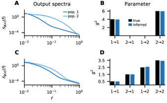
Figure 3: Maximum likelihood parameter estimation for two populations with different time constants $\tau_{1}=5$, $\tau_{2}=1$. A Output power spectra $\mathcal{S}_{\phi(x)}^{\alpha}(f)$ of two unconnected populations $g_{12}^{2}=g_{21}^{2}=0$ with $g_{11}^{2}=4$ and $g_{22}^{2}=6$. B Estimated (blue) and true (black) parameters corresponding to A. C Output power spectra of two connected populations with $g_{11}^{2}=0.5$, $g_{12}^{2}=1.5$, $g_{21}^{2}=2.5$, and $g_{22}^{2}=3.5$. D Estimated (blue) and true (black) parameters corresponding to C. Further parameters: $N_{1}=N_{2}=5,000$, $\phi(x)=\mathrm{erf}(\sqrt{\pi}x/2)$, $U(x)=\frac{1}{2}x^{2}$, and $D=0$; simulation parameters as in Fig. 1.

For multiple populations, any population-averaged observable can be obtained from the empirical measure $\mu^{\alpha}(y)=\frac{1}{N_{\alpha}}\sum_{i=1}^{N_{\alpha}}\delta(x_{i}^{\alpha}-y)$. The joint distribution of all population-specific empirical measures $\{\mu^{\circ}\}$ is determined by the rate function (Appendix D)

$$H(\{\mu^{\circ}\})=\sum_{\alpha}\gamma_{\alpha}\int\mathcal{D}x\,\mu^{\alpha}(x)\,\ln\frac{\mu^{\alpha}(x)}{\left\langle\delta(\tau_{\alpha}\dot{x}+U_{\alpha}^{\prime}(x)-\eta_{\alpha})\right\rangle_{\eta_{\alpha}}}\,,$$ (14)

where $\gamma_{\alpha}=N_{\alpha}/N$ and $\eta_{\alpha}$ is a zero-mean Gaussian process with

$$C_{\eta}^{\alpha}(t_{1},t_{2}) =2D_{\alpha}\delta(t_{1}-t_{2})$$

$$+\sum_{\beta}g_{\alpha\beta}^{2}\int\mathcal{D}x\,\mu^{\beta}(x)\phi(x(t_{1}))\phi(x(t_{2})).$$ (15)

Again, the rate function can be interpreted as a log-likelihood; its derivative leads to (Appendix E1)

$$\mathcal{S}_{\tau_{\alpha}\dot{x}+U_{\alpha}^{\prime}(x)}^{\alpha}(f) =2D_{\alpha}+\sum_{\beta}g_{\alpha\beta}^{2}\mathcal{S}_{\phi(x)}^{\beta}(f),$$ (16)

which generalizes Eq. (12) to multiple populations.

Using Eq. (16), the inferred connectivity $g_{\alpha\beta}$ matches the ground truth well; accordingly, two unconnected populations (Fig. 3A,B) can be clearly distinguished from a more involved network where one population ($\alpha=1$) is only active due to the recurrent input from the other population ($\alpha=2$, Fig. 3C,D). The method can thus distinguish intrinsically generated activity from a case where activity is driven from outside the network. However, inference of a unique set of parameters is only possible if the output spectra $\mathcal{S}_{\phi(x)}^{\alpha}(f)$ differ sufficiently across $\alpha$. If the output spectra match closely, Eq. (16) leads to a degenerate set of solutions that satisfy $\sum_{\beta}g_{\alpha\beta}^{2}=\mathrm{const.}$ and are all equally likely given the data (Appendix E2).

Discussion.–

In this Letter, we found a tight link between the field theoretical approach to neuronal networks and its counterpart based on large deviations theory. We obtained the rate function of the empirical measure for the widely used and analytically solvable model of a recurrent neuronal network [4] by field-theoretical methods. This rate function generalizes the seminal result by Ben Arous and Guionnet [11, 12] to arbitrary potentials, transfer functions, and multiple populations. Intriguingly, our derivation elucidates that the rate function is identical to the effective action and takes the form of a Kullback–Leibler divergence, akin to Sanov’s theorem for sums of i.i.d. random variables [22, 21]. The rate function can thus be interpreted as a distance between an empirical measure, for example given by data, and the activity statistics of the network model. This result allows us to address the inverse problem of inferring the parameters of the connectivity and external input from a set of trajectories and to determine the potential and the transfer function.

We here restricted the analysis to networks with independently drawn random weights with zero mean. Since correlated weights have a profound impact on the dynamics that can be captured using both field theory [25] and large deviations theory [26, 27], it is an interesting challenge to extend the analysis in this direction. Likewise, synaptic weights with non-vanishing mean, as they appear in sparsely-connected networks, present an interesting extension, because they promote fluctuation-driven states when feedback is sufficiently positive. Another important deviation from independent weights in biological neural networks are motifs [28], which pose a significant challenge already for the field-theoretical approach [29]. Beyond the weight statistics, we assumed that the dynamics are governed by the first-order differential equation (1). Indeed, the field-theoretical approach can be generalized to a much broader class of dynamics that do not necessarily possess an action [30]; hence, it seems possible to also derive large deviations results for more general dynamics. In this regard, the extension to spiking networks is a particularly interesting but also challenging future direction. Whether the model, Eq. (1), with its current limitations—the independent weights and the first-order dynamics—allows accurate inference of network parameters from cortical recordings is an intriguing question for further research.

The unified description of random networks by statistical field theory and large deviations theory opens the door to established techniques from either domain to capture beyond mean-field behavior. Such corrections are important for small or sparse networks with non–vanishing mean connectivity, to explain correlated neuronal activity, and to study information processing in finite-size networks with realistically limited resources. We here make a first step by computing fluctuation corrections from the rate function. The quantitative theory explains near-critical fluctuations for $g\in[1,1+\delta(N)]$ and we discover that expansive gain functions, as found in biology [31], lead to qualitatively different collective behavior than the well-studied contractive sigmoidal ones: The former feature meta–stable network states with noise-induced first order transitions between them; the latter allow for only a single solution and show second order phase transitions.