An Independence Test Based on Recurrence Rates. An empirical study and applications to real data

Juan Kalemkerian
Universidad de la República, Facultad de Ciencias

Diego Fernández
Universidad de la República, Facultad de Ciencias Económicas
y Administración
Abstract

In this paper we propose several variants to perform the independence test between two random elements based on recurrence rates. We will show how to calculate the test statistic in each one of these cases. From simulations we obtain that in high dimension, our test clearly outperforms, in almost all cases, the other widely used competitors. The test was performed on two data sets including small and large sample sizes and we show that in both cases the application of the test allows us to obtain interesting conclusions.

Keywords: independence tests, recurrence rates, U-process. 62H15, 62H20

1 Introduction

Let $\left(X_{1},Y_{1}\right),\left(X_{2},Y_{2}\right),...,\left(X_{n},Y_{n}\right)$ be an i.i.d. sample of $\left(X,Y\right),$ $X\in S_{X}$ and $Y\in S_{Y}$, where $S_{X}$ and $S_{Y}$ are metric spaces. Consider the hypothesis $H_{0}$ which asserts that $X$ and $Y$ are independent random elements: this is the so called independence test. Independence tests were developed at first for the case of $S_{X}=S_{Y}=\mathbb{R}$, based on the pioneering work of Galton [7] and Pearson [19] (this is the famous correlation test, which is widely used today). The limitations of this hypothesis test are well known and have motivated several different proposals in this topic, such as the classical rank test (e.g. Spearman, [22], Kendall, [16], and Blomqvist, [4]). The independence of random vectors was addressed for the first time in Wilks [26]. Several independence tests between random vectors have been proposed by now, see, for example, [8], [17], [3] and [2]. Gretton et al. [10] propose a universally consistent test based on Hilbert–Schmidt norms. This test has become very popular, and works well for random vectors in high dimensions. Another consistent and very popular test for random vectors is proposed by Székely et al. [24, 25], which defines the concept of distance covariance. It has been used and has had a considerable impact from the moment that it was proposed. This test has been adapted to work in high dimensions. Not many independence test have been developed for random elements where $X$ and $Y$ lie in an arbitrary metric space. Recently, in [14], an independence test based on recurrence rates was proposed. This test is based on the following simple idea: if $X$ and $Y$ are independent, then $d_{X}(X_{1},X_{2})$ and $d_{Y}(Y_{1},Y_{2})$ are independent for all i.i.d. $(X_{1},Y_{1}),(X_{2},Y_{2})$ with the same distribution as $(X,Y)$, where $d_{X}$ and $d_{Y}$ are the distance functions between elements of $S_{X}$ and $S_{Y}$, respectively. The authors proposed working with an $L^{2}$-Cramér–von Mises functional. On the one hand, from the theoretical point of view, this test is interesting because it does not need any assumptions on the topological structure of the metric spaces (e.g. assuming that they are Banach spaces), and in [14] can be found the first study where the mathematical properties of the recurrence rates were established. Marwan [18] gives a historical review of recurrence plots techniques, together with everything developed from them. However, the potential of these techniques has not  yet been studied in depth from the point of view of mathematical statistics. On the other hand, from the practical point of view, this test is interesting because it can be used for $X$ and $Y$ lying in spaces of any dimension, and in [14] a power comparison shows the very good performance of this test compared to others widely used for random variables and random vectors.

In the present paper we will show, using a power comparison, that the independence test of recurrence rates in high dimension outperforms the other competing tests in almost all cases, and we will study the incidence of the distance functions considered ($d_{X}$ and $d_{Y}$) in the performance of the test. As expected, we will show that the test statistic in high dimension has some sensitivity to the choice of the distance function, $d_{X}$ or $d_{Y}$. Also, we will propose and compare other functionals to be taken into account, such as an $L^{1}$-Cramér–von Mises functional and a Kolmogorov–Smirnov functional, and we will show how to compute the statistic in each case. Lastly, we will present applications of the test to two real data sets.

The rest of this paper is organized as follows. In Section 2 we define the procedure to test $H_{0}$ vs $H_{1}$ proposed in [14] and we present the definition of the test statistics based on a functional of the $L^{1}$-Cramér–von Mises type, and the statistics based on a functional of the Kolmogorov–Smirnov type, and three different distances to use in $S_{X}$ and $S_{Y}$. In Section 3, we show how to compute the different statistics presented in Section 2. In Section 4 we present a simulation study that compares, under several alternatives, the powers of the different tests of recurrence rates when varying the test statistics and the distance functions. In Section 5, we compare the performance of the recurrence test of independence with others in high dimension and we show that our test clearly outperforms the rest in almost all cases. In Section 6, we present two applications of the recurrence test of independence to meteorological data, one of them with small sample size and the second on involving a huge data set, and we show the ability of the recurrence rate test to obtain interesting conclusions. Some concluding remarks are given in Section 7 and the proof of the validity of the formulas established in Section 3 can be found in Section 8.

2 Test Approach and Different Statistics to Consider

Let $\left(X_{1},Y_{1}\right),\left(X_{2},Y_{2}\right),...,\left(X_{n},Y_{n}\right)$ be i.i.d. samples of $\left(X,Y\right)$ where $X\in S_{X},$ $Y\in S_{Y}$, $S_{X}$ and $S_{Y}$ are metric spaces, and suppose given $r,s>0.$ To simplify the notation and without risk of confusion, we will use the same letter $d$ for the distance function on both metric spaces, $S_{X}$ and $S_{Y}$.

We define the recurrence rate for the sample of $X$ and $Y$ as

$$RR_{n}^{X}(r):=\frac{1}{n^{2}-n}\sum_{i\neq j}\mathbf{1}_{\left\{d\left(X_{i},X_{j}\right)<r\right\}},\ \ \ \ \ RR_{n}^{Y}(s):=\frac{1}{n^{2}-n}\sum_{i\neq j}\mathbf{1}_{\left\{d\left(Y_{i},Y_{j}\right)<s\right\}},$$

respectively, and the joint recurrence rate for $\left(X,Y\right)$ as

$$RR_{n}^{X,Y}(r,s):=\frac{1}{n^{2}-n}\sum_{i\neq j}\mathbf{1}_{\left\{d\left(X_{i},X_{j}\right)<r\text{ },\text{ }d\left(Y_{i},Y_{j}\right)<s\right\}}.$$

If we define $p_{X}(r):=P\left(d\left(X_{1},X_{2}\right)<r\right)$ the probability that the distance between any two elements of the sample $X$ is less than $r$ and $p_{X,Y}(r,s):=P\left(d\left(X_{1},X_{2}\right)<r,\text{ }d\left(Y_{1},Y_{2}\right)<s\right)$ the joint probability that the distance between any two elements of the sample $X$ is less than $r$ and any two elements of the sample $Y$ is less than $s,$ the strong law of large numbers for $U$-statistics ([11]) allows us to affirm that for any $r,s>0$,

$$RR_{n}^{X}(r)\overset{a.s.}{\rightarrow}p_{X}(r),\ \ RR_{n}^{Y}(s)\overset{a.s.}{\rightarrow}p_{Y}(s)\ \ \text{and}\ \ RR_{n}^{X,Y}(r,s)\overset{a.s.}{\rightarrow}p_{X,Y}(r,s).$$ (1)

We want to test $H_{0}:$ $X$ and $Y$ are independent, against $H_{1}:$ $H_{0}$ does not hold.

If $H_{0}$ is true, then $p_{X,Y}(r,s)=p_{X}(r)p_{Y}(s)$ for all $r,s>0$, and we expect that if $n$ is large, $RR_{n}^{X,Y}(r,s)\cong RR_{n}^{X}(r)RR_{n}^{Y}(s)$ for any $r,s>0.$ In [14] it is proposed to reject $H_{0}$ when $T_{n}>c$, where

$$T_{n}:=n\int_{0}^{+\infty}\int_{0}^{+\infty}\left(RR_{n}^{X,Y}(r,s)-RR_{n}^{X}(r)RR_{n}^{Y}(s)\right)^{2}dG(r,s),$$ (2)

where $c$ is a constant and $G$ is a properly chosen distribution function. Observe that $T_{n}$ is a functional of the $L^{2}$ Cramér–von Mises type applied to the process $\{E_{n}(r,s)\}_{r,s>0}$ where

$$E_{n}(r,s):=\sqrt{n}\left(RR_{n}^{X,Y}(r,s)-RR_{n}^{X}(r)RR_{n}^{Y}(s)\right).$$ (3)

The theoretical results established in [14] about the process defined in (3), are valid for any distance functions $d_{X}$ and $d_{Y}$, and remains valid if we consider other continuous functionals such as an $L^{1}$-Cramér–von Mises type or one of Kolmogorov–Smirnov type.

If $\left(X_{1},Y_{1}\right),\left(X_{2},Y_{2}\right),...,\left(X_{n},Y_{n}\right)$ are i.i.d. in $S_{X}\times S_{Y},$ we will compare the $T_{n}$ statistic proposed in [14], which we will call $T_{n}^{(2)}$, defined by

$$T_{n}^{(2)}:=n\int_{0}^{+\infty}\int_{0}^{+\infty}\left(RR_{n}^{X,Y}\left(r,s\right)-RR_{n}^{X}\left(r\right)RR_{n}^{Y}\left(s\right)\right)^{2}dG(r,s)$$

with the statistics defined as

$$T_{n}^{\left(1\right)}:=\sqrt{n}\int_{0}^{+\infty}\int_{0}^{+\infty}\left|RR_{n}^{X,Y}\left(r,s\right)-RR_{n}^{X}\left(r\right)RR_{n}^{Y}\left(s\right)\right|dG(r,s)$$

and

$$T_{n}^{\left(\infty\right)}:=\sqrt{n}\sup_{r,s>0}\left|RR_{n}^{X,Y}\left(r,s\right)-RR_{n}^{X}\left(r\right)RR_{n}^{Y}\left(s\right)\right|.$$

Observe that in the general case in which $X$ and $Y$ lie in metric spaces $\left(S_{X},d_{X}\right)$ and $\left(S_{Y},d_{Y}\right)$, the statistics $T_{n}^{\left(1\right)},T_{n}^{\left(2\right)}$ and $T_{n}^{\left(\infty\right)}$ depend on the distance functions $d_{X}$ and $d_{Y}.$ In Section 4 we will compare the power under several alternative tests based on $T_{n}^{\left(1\right)},T_{n}^{\left(2\right)}$ and $T_{n}^{\left(\infty\right)}$ for different distance functions $d_{X}$ and $d_{Y}.$

In the case in which $X$ and $Y$ are discrete time series, we will use the classical $l^{1},l^{2}$ and $l^{\infty}$ distances, that is, $d_{X}\left(x,x^{\prime}\right)=\sum_{n\geq 1}\left|x_{n}-x_{n}^{\prime}\right|,$ $d_{X}\left(x,x^{\prime}\right)=\sqrt{\sum_{n\geq 1}\left(x_{n}-x_{n}^{\prime}\right)^{2}}$ and $d_{X}\left(x,x^{\prime}\right)=\sup_{n\geq 1}\left|x_{n}-x_{n}^{\prime}\right|$ and analogously for $d_{Y}.$ Analogously, when $X$ and $Y$ are continuous time series, we will use the classical $L^{1},L^{2},L^{\infty}$ distances, that is, $d_{X}\left(x,x^{\prime}\right)=\int_{-\infty}^{+\infty}\left|x(t)-x^{\prime}(t)\right|dt,$ $d_{X}\left(x,x^{\prime}\right)=\sqrt{\int_{-\infty}^{+\infty}\left(x(t)-x^{\prime}(t)\right)^{2}dt}$ and $d_{X}\left(x,x^{\prime}\right)=\sup_{t\in\mathbb{R}}\left|x(t)-x^{\prime}(t)\right|.$ We will use the notation $T_{n}^{\left(i,j\right)}$ where $i,j=1,2,\infty$ for the statistic $T_{n}^{\left(i\right)}$ where the distance functions used are the $l^{j}$ $\left(\text{or }L^{j}\right)$ distance.

In all cases, as proposed in [14], we will use a weight function $G$ such that $dG(r,s)=g_{1}(r)g_{2}(s)drds$ where $g_{1}$ and $g_{2}$ are $g_{1}\left(z\right)=\varphi\left(\frac{z-\mu_{X}}{\sigma_{X}}\right)$ with $\varphi$ being the density function of an $N\left(0,1\right)$ random variable and $\mu_{X}=\mathbb{E}\left(d\left(X_{1},X_{2}\right)\right),$ $\sigma_{X}^{2}=\mathbb{V}\left(d\left(X_{1},X_{2}\right)\right)$ being $X_{1},X_{2}$ independent random variables with the same distribution as $X.$ Analogously, $g_{2}\left(t\right)=\varphi\left(\frac{t-\mu_{Y}}{\sigma_{Y}}\right).$ In practice $\mu_{X}$ and $\sigma_{X}$ are unknown, but they can be estimated naturally by $\widehat{\mu}_{X}=\frac{1}{N}\sum_{i\neq j}d\left(X_{i},X_{j}\right)$ and $\widehat{\sigma}_{X}^{2}=\frac{1}{N}\sum_{i\neq j}\left(d\left(X_{i},X_{j}\right)-\widehat{\mu}_{X}\right)^{2}$ where $N=n(n-1)$, and analogously with $\widehat{\mu}_{Y}$ and $\widehat{\sigma}_{Y}^{2}.$

3 Computing the Statistics

Given $\left(X_{1},Y_{1}\right),\left(X_{2},Y_{2}\right),...,\left(X_{n},Y_{n}\right)$ i.i.d. in $S_{X}\times S_{Y},$ and choosen the weight functions $g_{1}$, $g_{2}$ to be used, the statistic $T_{n}^{(1)},T_{n}^{(2)}$ and $T_{n}^{(\infty)}$ can be computed in the steps that indicated the following three propositions.

Proposition 1.

Calculation of $T_{n}^{(2)}$.
Step 1. Compute $d\left(X_{i},X_{j}\right)$ and $d\left(Y_{i},Y_{j}\right)$ for all $i,j\in\left\{1,2,3,...,n\right\}$ where $i\neq j$ and put $N=n(n-1).$

Step 2. Re-order $\left\{d\left(X_{i},X_{j}\right)\right\}_{i\neq j}$ as $Z_{1},Z_{2},...,Z_{N}$ such that $Z_{1}<Z_{2}<...<Z_{N}$ and $\left\{d\left(Y_{i},Y_{j}\right)\right\}_{i\neq j}$ as $T_{1},T_{2},...,T_{N}$ maintaining the same indexing as $Z^{\prime}s$ (that is, if $d\left(X_{i},X_{j}\right)=Z_{h}$ then $d\left(Y_{i},Y_{j}\right)=T_{h}$).

Step 3. Compute the order statistics for $T^{\prime}s,$ that is, $T_{1}^{\ast}<T_{2}^{\ast}<...<T_{N}^{\ast}.$

Step 4. Compute

$$A_{n}=\frac{1}{N^{2}}\sum_{i=1}^{N}\sum_{j=1}^{N}\left(1-G_{1}\left(\max\left\{Z_{i},Z_{j}\right\}\right)\right)\left(1-G_{2}\left(\max\left\{T_{i},T_{j}\right\}\right)\right),$$
$$B_{n}=\left(1-\frac{1}{N^{2}}\sum_{i=1}^{N}\left(2i-1\right)G_{1}\left(Z_{i}\right)\right)\left(1-\frac{1}{N^{2}}\sum_{i=1}^{N}\left(2i-1\right)G_{2}\left(T_{i}^{\ast}\right)\right),$$
$$C_{n}=\frac{1}{N^{3}}\sum_{i=1}^{N}\sum_{j=1}^{N}\sum_{k=1}^{N}\left(1-G_{1}\left(\max\left\{Z_{i},Z_{j}\right\}\right)\right)\left(1-G_{2}\left(\max\left\{T_{i},T_{k}\right\}\right)\right).$$

Step 5. Compute

$$T_{n}^{(2)}=n(A_{n}+B_{n}-2C_{n}).$$
Proposition 2.

Calculation of $T_{n}^{(1)}$.
Step 1. Compute $d\left(X_{i},X_{j}\right)$ and $d\left(Y_{i},Y_{j}\right)$ for all $i,j\in\left\{1,2,3,...,n\right\}$ where $i\neq j$ and put $N=n(n-1).$

Step 2. Re-order $\left\{d\left(X_{i},X_{j}\right)\right\}_{i\neq j}$ as $Z_{1},Z_{2},...,Z_{N}$ such that $Z_{1}<Z_{2}<...<Z_{N}$ and $\left\{d\left(Y_{i},Y_{j}\right)\right\}_{i\neq j}$ as $T_{1},T_{2},...,T_{N}$ maintaining the same indexing as $Z^{\prime}s$ (that is, if $d\left(X_{i},X_{j}\right)=Z_{h}$ then $d\left(Y_{i},Y_{j}\right)=T_{h}$).

Step 3. Compute the order statistics for $T^{\prime}s,$ that is, $T_{1}^{\ast}<T_{2}^{\ast}<...<T_{N}^{\ast}.$

Step 4. For each $h,j\in\left\{1,2,3,...,N-1\right\}$ compute $c(h,j)=\sum_{i=1}^{h}\mathbf{1}_{\left\{T_{i}<T_{j+1}^{\ast}\right\}}$, that is, the number of elements of the vector $\left(T_{1},T_{2},...,T_{h}\right)$ that are less than $T_{j+1}^{\ast}$ for $h,j=1,2,3,...,N-1.$

Step 5. Compute

$$T_{n}^{\left(1\right)}=\frac{\sqrt{n}}{N}\sum_{h,j=1}^{N-1}\left(G_{1}\left(Z_{h+1}\right)-G_{1}\left(Z_{h}\right)\right)\left(G_{2}\left(T_{j+1}^{\ast}\right)-G_{2}\left(T_{j}^{\ast}\right)\right)\left|c(h,j)-\frac{jh}{N}\right|.$$
Proposition 3.

Calculation of $T_{n}^{(\infty)}$.
Step 1. Compute $d\left(X_{i},X_{j}\right)$ and $d\left(Y_{i},Y_{j}\right)$ for all $i,j\in\left\{1,2,3,...,n\right\}$ where $i\neq j$ and put $N=n(n-1).$

Step 2. Re-order $\left\{d\left(X_{i},X_{j}\right)\right\}_{i\neq j}$ as $Z_{1},Z_{2},...,Z_{N}$ such that $Z_{1}<Z_{2}<...<Z_{N}$ and $\left\{d\left(Y_{i},Y_{j}\right)\right\}_{i\neq j}$ as $T_{1},T_{2},...,T_{N}$ maintaining the same indexing as $Z^{\prime}s$ (that is, if $d\left(X_{i},X_{j}\right)=Z_{h}$ then $d\left(Y_{i},Y_{j}\right)=T_{h}$).

Step 3. Compute the order statistics for $T^{\prime}s,$ that is, $T_{1}^{\ast}<T_{2}^{\ast}<...<T_{N}^{\ast}.$

Step 4. Compute the $\left(N-1\right)\times\left(N-1\right)$ matrix $C$ such that

$$C_{ij}=\left|\sum_{k=1}^{N}\mathbf{1}_{\left\{Z_{k}\leq Z_{i},\text{ }T_{k}\leq T_{j}^{\ast}\right\}}-\frac{ij}{N}\right|.$$

Step 5. Compute

$$T_{n}^{\left(\infty\right)}=\frac{\sqrt{n}}{N}\max_{i,j}C_{ij}.$$

4 Simulation Study

When $X$ and $Y$ lie in high dimensional spaces, it is interesting to analyse the performance of the test statistics $T_{n}^{(1)},T_{n}^{(2)}$ and $T_{n}^{(\infty)}$ for different distance functions $d_{X}$ and $d_{Y}$. In this section we will compare the power of the $9$ test statistics $T_{n}^{(i,j)}$ for $i,j=1,2,\infty$ in the cases in which $X$ and $Y$ are discrete and continuous time series under several alternatives. In all cases we will use the same distance function for $X$ and $Y$, that is, if $X$ and $Y$ are discrete time series, then we will use $l^{j}$ for both $X$ and $Y$ for $j=1,2,\infty$, and analogously in the case in which $X$ and $Y$ are continuous time series. In all cases, $X$ and $Y$ are time series of length $100$ and the power (due to the computational cost) was calculated at the $5\%$ level from $500$ replications. Every $p$-value was calculated by a permutation method (as suggested in [14]) for $100$ replications.

4.1 The discrete case
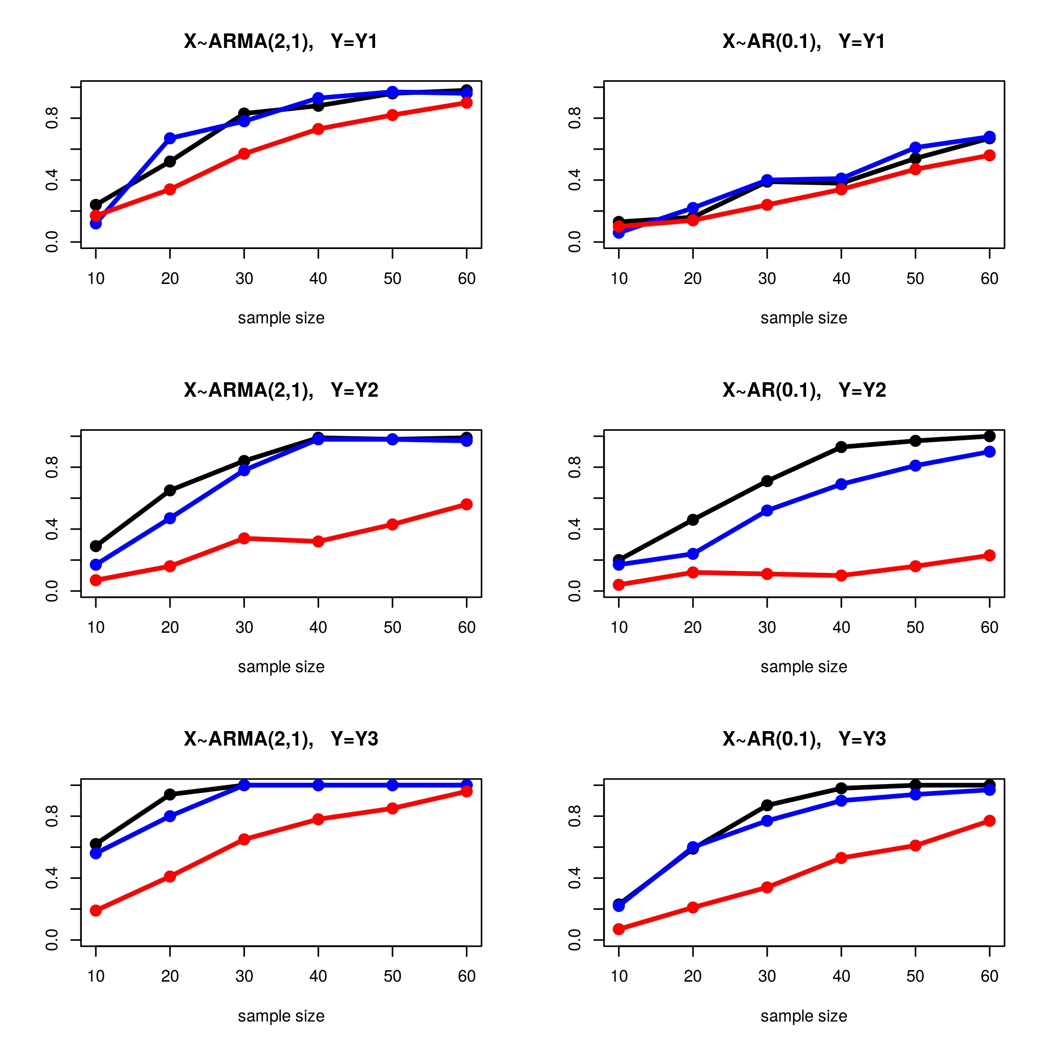
We analyse two scenarios for $X$: one of them is when $X$ is AR$(1)$ where $\phi=0.1$, which we call simply AR$(0.1)$ and the second case, is when $X$ is ARMA$(2,1)$ with parameters $\phi=(0.2,0.5)$ and $\theta=0.2$. In both cases we consider three possible $Y$: $Y_{1}=X^{2}+3\varepsilon$, $Y_{2}=\sqrt{|X|}+\sigma\varepsilon$ where $\sigma^{2}$ means the variance of $\sqrt{|X|}$ and $Y_{3}=\varepsilon X$. In all cases, $\varepsilon$ is a standard Gaussian white noise $(N(0,1))$ independent of $X$. In Table 1 and Table 2 we show the power for $n=30$ and $n=50$, respectively, in the case in which $X$ is an AR$(0.1)$ process for the 9 tests considered. Similarly Table 3 and Table 4 show the power for the case in which $X$ is an ARMA$(2,1)$ process. Tables 1–4 do not show important differences between using $T_{n}^{(2)}$, $T_{n}^{(1)}$ or $T_{n}^{(\infty)}$. In Figure 1 we show the power as a function of sample size, where the statistic considered is $T_{n}^{(2)}$, that is $T_{n}^{(2,1)}$, $T_{n}^{(2,2)}$ and $T_{n}^{(2,\infty)}$. The behaviour of $T_{n}^{(1)}$ and $T_{n}^{(2)}$ is similar. Figure 1 suggest that the power increases as the distance function considered goes from $d_{\infty}$ ($l^{\infty}$ distance) to $d_{1}$ ($l^{1}$ distance). Also for the alternative $Y=Y_{2}$, the statistic based on the $l^{\infty}$ distance has difficulties in detecting the dependence between $X$ and $Y$ (which grows very slowly as $n$ increases), while for $n=60$ the power of the test based on $l^{1}$ or $l^{2}$ distances is near unity.

Table 1: Comparison of powers, at the $5\%$ level, for the different tests, where $X$ is AR$(0.1)$ and $Y_{1}=X^{2}+3\varepsilon$, $Y_{2}=\sqrt{|X|}+\sigma\varepsilon$, $Y_{3}=\varepsilon X$ for sample size of $n=30$.
$n=30$ $T_{n}^{(1,1)}$ $T_{n}^{(1,2)}$ $T_{n}^{(1,\infty)}$ $T_{n}^{(2,1)}$ $T_{n}^{(2,2)}$ $T_{n}^{(2,\infty)}$ $T_{n}^{(\infty,1)}$ $T_{n}^{(\infty,2)}$ $T_{n}^{(\infty,\infty)}$
$Y=Y_{1}$ 0.39 0.40 0.29 0.39 0.40 0.24 0.32 0.28 0.16
$Y=Y_{2}$ 0.45 0.22 0.10 0.71 0.52 0.11 0.69 0.19 0.05
$Y=Y_{3}$ 0.91 0.79 0.28 0.87 0.77 0.34 0.92 0.77 0.27
Table 2: Comparison of powers, at the $5\%$ level, for the different tests, where $X$ is AR$(0.1)$ and $Y_{1}=X^{2}+3\varepsilon$, $Y_{2}=\sqrt{|X|}+\sigma\varepsilon$, $Y_{3}=\varepsilon X$ for sample size of $n=50$.
$n=50$ $T_{n}^{(1,1)}$ $T_{n}^{(1,2)}$ $T_{n}^{(1,\infty)}$ $T_{n}^{(2,1)}$ $T_{n}^{(2,2)}$ $T_{n}^{(2,\infty)}$ $T_{n}^{(\infty,1)}$ $T_{n}^{(\infty,2)}$ $T_{n}^{(\infty,\infty)}$
$Y=Y_{1}$ 0.90 0.92 0.74 0.54 0.59 0.47 0.49 0.57 0.34
$Y=Y_{2}$ 0.34 0.50 0.38 0.97 0.81 0.16 0.92 0.89 0.79
$Y=Y_{3}$ 1.00 0.94 0.64 1.00 0.94 0.61 0.99 0.92 0.57
Table 3: Comparison of powers, at the $5\%$ level, for the different tests, where $X$ is ARMA$(2,1)$ and $Y_{1}=X^{2}+3\varepsilon$, $Y_{2}=\sqrt{|X|}+\sigma\varepsilon$, $Y_{3}=\varepsilon X$ for sample size of $n=30$.
$n=30$ $T_{n}^{(1,1)}$ $T_{n}^{(1,2)}$ $T_{n}^{(1,\infty)}$ $T_{n}^{(2,1)}$ $T_{n}^{(2,2)}$ $T_{n}^{(2,\infty)}$ $T_{n}^{(\infty,1)}$ $T_{n}^{(\infty,2)}$ $T_{n}^{(\infty,\infty)}$
$Y=Y_{1}$ 0.85 0.82 0.53 0.83 0.78 0.57 0.77 0.85 0.47
$Y=Y_{2}$ 0.56 0.27 0.08 0.84 0.78 0.34 0.49 0.34 0.08
$Y=Y_{3}$ 1.00 1.00 0.93 0.99 0.93 0.50 0.96 0.88 0.23
Table 4: Comparison of powers, at the $5\%$ level, for the different tests, where $X$ is ARMA$(2,1)$ and $Y_{1}=X^{2}+3\varepsilon$, $Y_{2}=\sqrt{|X|}+\sigma\varepsilon$, $Y_{3}=\varepsilon X$ for sample size of $n=50$.
$n=50$ $T_{n}^{(1,1)}$ $T_{n}^{(1,2)}$ $T_{n}^{(1,\infty)}$ $T_{n}^{(2,1)}$ $T_{n}^{(2,2)}$ $T_{n}^{(2,\infty)}$ $T_{n}^{(\infty,1)}$ $T_{n}^{(\infty,2)}$ $T_{n}^{(\infty,\infty)}$
$Y=Y_{1}$ 0.98 0.98 0.82 0.96 0.97 0.82 0.96 0.96 0.82
$Y=Y_{2}$ 0.76 0.48 0.04 0.98 0.98 0.43 0.65 0.43 0.03
$Y=Y_{3}$ 1.00 1.00 0.74 1.00 1.00 0.77 1.00 1.00 0.75
Refer to caption
Figure 1: Power at $5\%$ level under several alternatives for the statistic $T_{n}^{(2)}$ using Manhattan distance ($T_{n}^{(2,1)}$ in black), Euclidean distance ($T_{n}^{(2,2)}$ in blue) and maximum distance ($T_{n}^{(2,\infty)}$ in red). $Y_{1}$, $Y_{2}$ and $Y_{3}$ are defined in Tables 1–4.

4.2 The continuous case

In this subsection, we will take X𝑋X to be a fractional Brownian motion with σ=1𝜎1\sigma=1 observed in [0,1]01[0,1] (at times 0,1/100,2/100,,99/100011002100991000,1/100,2/100,...,99/100) for H=0.5𝐻0.5H=0.5 (standard Brownian motion) and H=0.7𝐻0.7H=0.7. We consider 777 dependence cases between X𝑋X and Y𝑌Y. The first three are for the case in which X𝑋X is a standard Brownian motion (Bm𝐵𝑚Bm) and the dependence is defined by Y1=X2+3εsubscript𝑌1superscript𝑋23𝜀Y_{1}=X^{2}+3\varepsilon, Y2=|X|+εsubscript𝑌2𝑋𝜀Y_{2}=\sqrt{|X|}+\varepsilon, Y3=εX+3εsubscript𝑌3𝜀𝑋3superscript𝜀Y_{3}=\varepsilon X+3\varepsilon^{\prime} where ε𝜀\varepsilon and εsuperscript𝜀\varepsilon^{\prime} are Gaussian white noises with σ=1𝜎1\sigma=1 such that X,ε𝑋𝜀X,\varepsilon and εsuperscript𝜀\varepsilon^{\prime} are independent. In the last 444 alternatives, we explore the power when Y𝑌Y is a linear functional of X𝑋X. More explicitly, we will consider the case in which Y𝑌Y is a fractional Ornstein–Uhlenbeck process driven by a Brownian motion (X𝑋X) for H=0.5𝐻0.5H=0.5 (Bm𝐵𝑚Bm) and fractional Brownian motion for H=0.7𝐻0.7H=0.7 (fBm𝑓𝐵𝑚fBm), which we call the OU𝑂𝑈OU and FOU𝐹𝑂𝑈FOU processes, respectively. A particular, a linear combination of FOU𝐹𝑂𝑈FOU, which we call FOU(2)𝐹𝑂𝑈2FOU(2), and whose definition, theoretical development and simulations are found in [13] and [12], is a particular case of the models proposed in [1]. More explicitly, the FOU𝐹𝑂𝑈FOU process is defined by Yt=σteλ(ts)𝑑Xssubscript𝑌𝑡𝜎superscriptsubscript𝑡superscript𝑒𝜆𝑡𝑠differential-dsubscript𝑋𝑠Y_{t}=\sigma\int_{-\infty}^{t}e^{-\lambda(t-s)}dX_{s} (where X={Xt}𝑋subscript𝑋𝑡X=\{X_{t}\} is an fBm𝑓𝐵𝑚fBm), and the FOU(2)𝐹𝑂𝑈2FOU(2) process is defined by Yt=λ1λ1λ2σteλ1(ts)𝑑Xs+λ2λ2λ1σteλ2(ts)𝑑Xssubscript𝑌𝑡subscript𝜆1subscript𝜆1subscript𝜆2𝜎superscriptsubscript𝑡superscript𝑒subscript𝜆1𝑡𝑠differential-dsubscript𝑋𝑠subscript𝜆2subscript𝜆2subscript𝜆1𝜎superscriptsubscript𝑡superscript𝑒subscript𝜆2𝑡𝑠differential-dsubscript𝑋𝑠Y_{t}=\dfrac{\lambda_{1}}{\lambda_{1}-\lambda_{2}}\sigma\int_{-\infty}^{t}e^{-\lambda_{1}(t-s)}dX_{s}+\dfrac{\lambda_{2}}{\lambda_{2}-\lambda_{1}}\sigma\int_{-\infty}^{t}e^{-\lambda_{2}(t-s)}dX_{s} (where X={Xt}𝑋subscript𝑋𝑡X=\{X_{t}\} is an fBm𝑓𝐵𝑚fBm). When H=0.5𝐻0.5H=0.5, we will call them simply the OU𝑂𝑈OU and OU(2)𝑂𝑈2OU(2) processes, as defined in [1]. Tables 5 and 6 gives us the power for n=30𝑛30n=30 and n=50𝑛50n=50, respectively, for the 777 alternatives. In these tables, Y4subscript𝑌4Y_{4} means an OU𝑂𝑈OU process driven by X𝑋X with parameters σ=1,λ=0.3formulae-sequence𝜎1𝜆0.3\sigma=1,\lambda=0.3. Similarly Y5subscript𝑌5Y_{5} is an FOU𝐹𝑂𝑈FOU process with parameters σ=1,H=0.7,λ=0.3formulae-sequence𝜎1formulae-sequence𝐻0.7𝜆0.3\sigma=1,H=0.7,\lambda=0.3, Y6OU(2)similar-tosubscript𝑌6𝑂𝑈2Y_{6}\sim OU(2) with parameters σ=1,λ1=0.3,λ2=0.8formulae-sequence𝜎1formulae-sequencesubscript𝜆10.3subscript𝜆20.8\sigma=1,\lambda_{1}=0.3,\lambda_{2}=0.8 and Y7FOU(2)similar-tosubscript𝑌7𝐹𝑂𝑈2Y_{7}\sim FOU(2) with parameters σ=1,H=0.7,λ1=0.3,λ2=0.8formulae-sequence𝜎1formulae-sequence𝐻0.7formulae-sequencesubscript𝜆10.3subscript𝜆20.8\sigma=1,H=0.7,\lambda_{1}=0.3,\lambda_{2}=0.8. In this paper we do not present the performance of the test for other choices of the parameters, because the behaviour is similar. As expected, for values of σ𝜎\sigma larger than 111, the dependence between X𝑋X and Y𝑌Y is more difficult to detect, and we need to increase the sample size. The same occurs if we take λ1subscript𝜆1\lambda_{1} near to λ2subscript𝜆2\lambda_{2} in OU(2)𝑂𝑈2OU(2) and FOU(2)𝐹𝑂𝑈2FOU(2). Tables 5 and 6 show, as in the discrete case, no substantial differences between the performance of the three statistics (Tn(1),Tn(2)superscriptsubscript𝑇𝑛1superscriptsubscript𝑇𝑛2T_{n}^{(1)},T_{n}^{(2)} or Tn()superscriptsubscript𝑇𝑛T_{n}^{(\infty)}). With respect to which distance between elements of X𝑋X and Y𝑌Y is more appropriate, Table 5 and Table 6 show that the Lsuperscript𝐿L^{\infty} distance performs poorly under the alternatives Y1,Y2subscript𝑌1subscript𝑌2Y_{1},Y_{2} and Y3subscript𝑌3Y_{3}, but better under alternatives Y4,Y5,Y6subscript𝑌4subscript𝑌5subscript𝑌6Y_{4},Y_{5},Y_{6} and Y7subscript𝑌7Y_{7}. The performance of the L1superscript𝐿1L^{1} and L2superscript𝐿2L^{2} distances is similar throughout the 777 
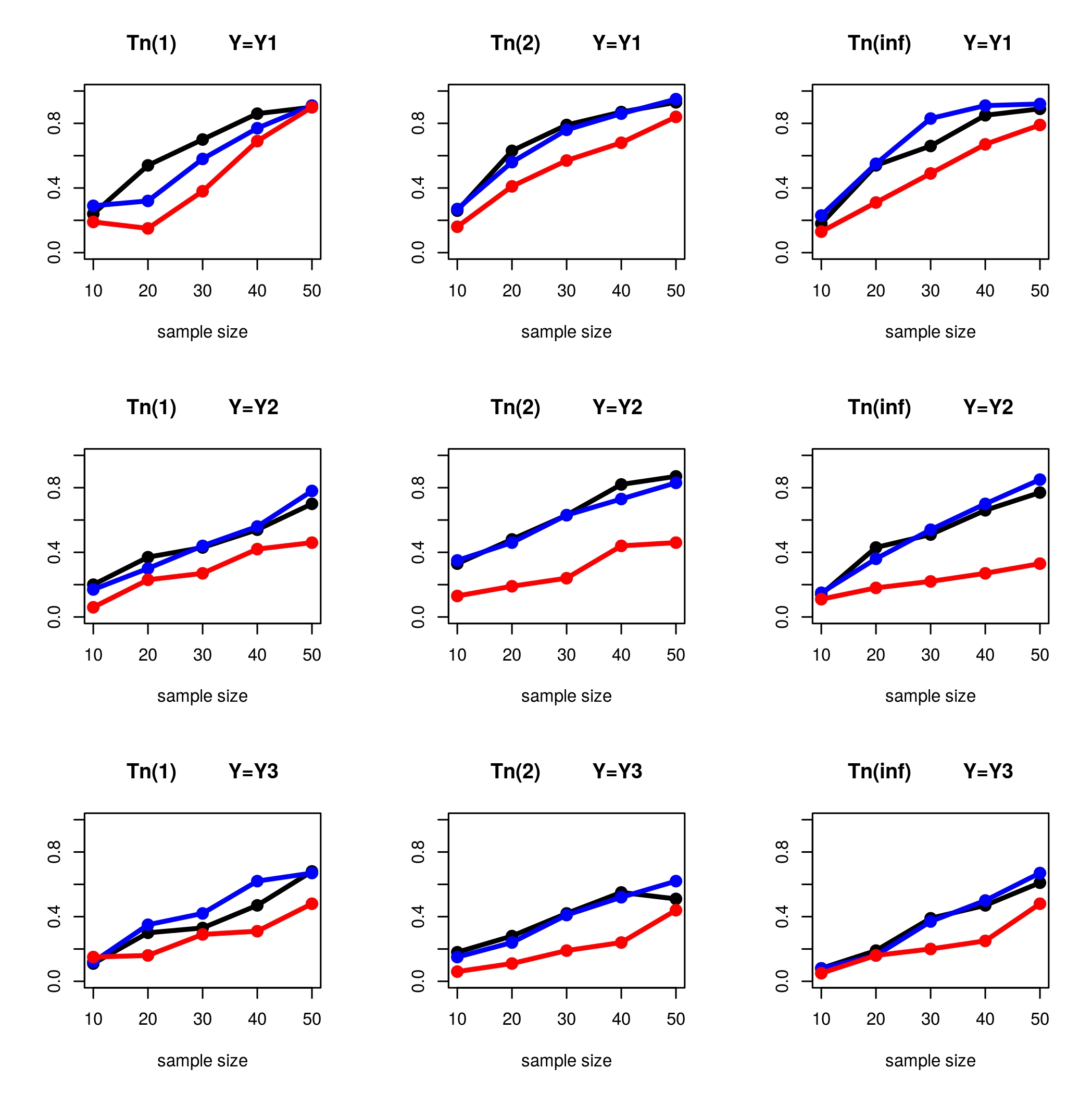
alternatives. Figure 2 expands the information given in Table 5 and Table 6 for the cases Y1,Y2subscript𝑌1subscript𝑌2Y_{1},Y_{2} and Y3subscript𝑌3Y_{3} because it shows us the power for the statistics Tn(i,j)superscriptsubscript𝑇𝑛𝑖𝑗T_{n}^{(i,j)} for i,j=1,2,formulae-sequence𝑖𝑗12i,j=1,2,\infty for sample sizes of n=10𝑛10n=10 to n=50𝑛50n=50. Figure 2 show clearly that the Lsuperscript𝐿L^{\infty} distance has a poorer performance than the L1superscript𝐿1L^{1} and L2superscript𝐿2L^{2} distances. 
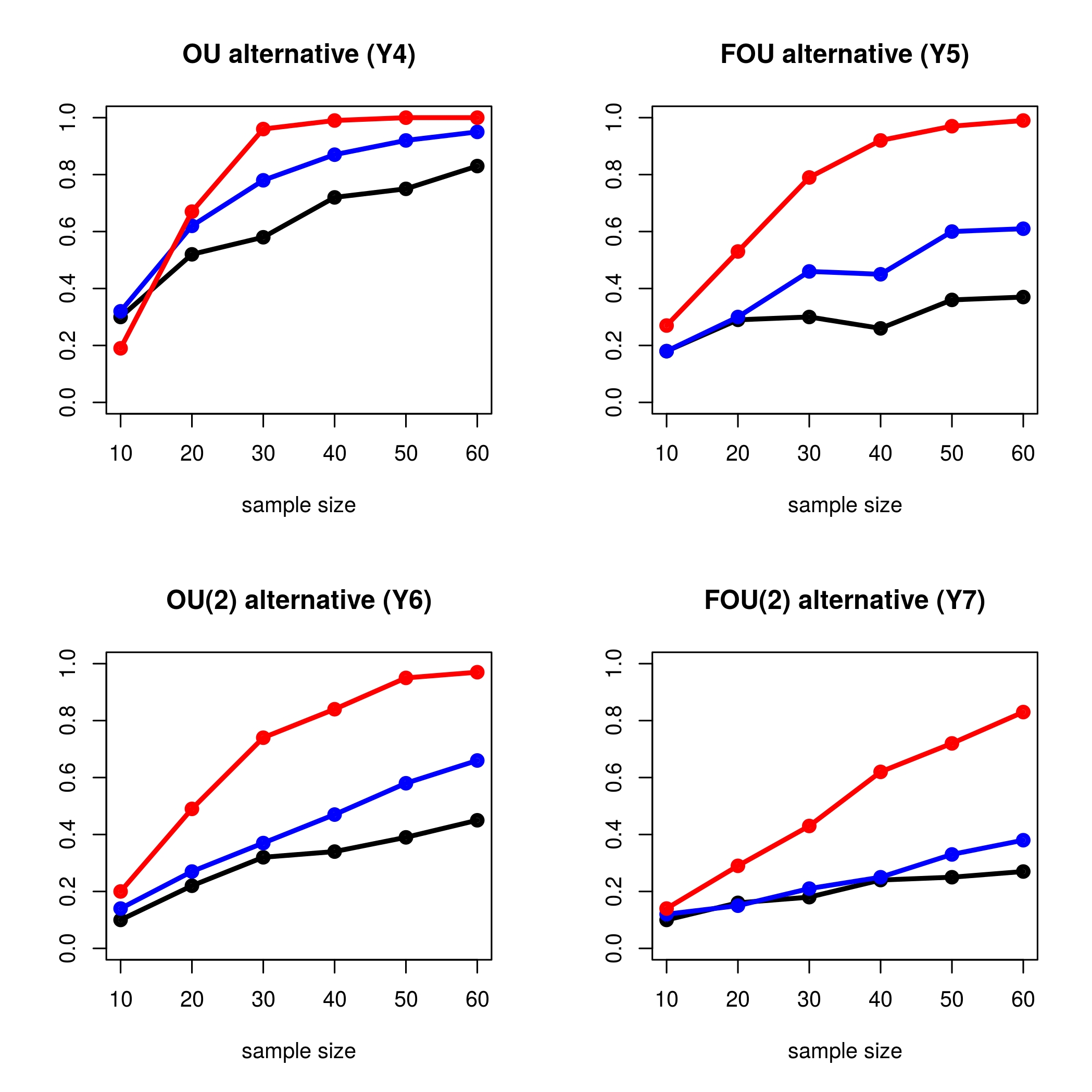
Figure 3 shows the power as a function of sample size for the statistic Tn(2)superscriptsubscript𝑇𝑛2T_{n}^{(2)} in the cases Y4,Y5,Y6subscript𝑌4subscript𝑌5subscript𝑌6Y_{4},Y_{5},Y_{6} and Y7subscript𝑌7Y_{7}. The behaviour of the statistics Tn(1)superscriptsubscript𝑇𝑛1T_{n}^{(1)} and Tn(2)superscriptsubscript𝑇𝑛2T_{n}^{(2)} is similar. Contrary to what happened in the cases Y1,Y2subscript𝑌1subscript𝑌2Y_{1},Y_{2} and Y3subscript𝑌3Y_{3}, the Lsuperscript𝐿L^{\infty} distance performs clearly better than the L1superscript𝐿1L^{1} and L2superscript𝐿2L^{2} distances. Also, Figure 3 show that the performance of the Tn(2)superscriptsubscript𝑇𝑛2T_{n}^{(2)} statistic increases as we move from the use of the L1superscript𝐿1L^{1} distance to the use of the Lsuperscript𝐿L^{\infty} distance. On the other hand, Figure 3 shows that the power in the case of the OU𝑂𝑈OU alternative is higher than for the OU(2)𝑂𝑈2OU(2) alternative (and the same for FOU𝐹𝑂𝑈FOU versus FOU(2)𝐹𝑂𝑈2FOU(2)), which is reasonable, because the dependence between X𝑋X and Y𝑌Y is simpler in the OU𝑂𝑈OU (FOU𝐹𝑂𝑈FOU) case than in the OU(2)𝑂𝑈2OU(2) (FOU(2)𝐹𝑂𝑈2FOU(2)) case. Also, the power in the OU𝑂𝑈OU (OU(2)𝑂𝑈2OU(2)) case is higher than in the FOU𝐹𝑂𝑈FOU (FOU(2)𝐹𝑂𝑈2FOU(2)) case, which is to be expected because when H=0.7𝐻0.7H=0.7, the fractional Brownian motion has a long range dependence, therefore it is reasonable that the dependence between X𝑋X and Y𝑌Y is more difficult to detect.
To conclude this section, observe that the test of independence based on recurrence rates has a power that grows as $n$ grows for the $9$ statistics considered, $T_{n}^{(i,j)}$ for $i,j=1,2,\infty$ (as expected according to the theory developed in [14]) in all the alternatives considered for both the discrete and the continuous cases. In most of the cases, the test has a power near to unity for moderately small sample sizes. Taking into account what was observed in this section, it can be said that there is no preference to use the test based on $T_{n}^{(1)},T_{n}^{(2)}$ or $T_{n}^{(\infty)}$, but in the three cases, in general the performance is better as the function distance goes from the $L^{1}$ ($l^{1}$) distance to the $L^{\infty}$ ($l^{\infty}$) distance in some cases, and in the opposite direction for other cases. Therefore, it can be suggested that one use the test statistic using the $L^{1}$ ($l^{1}$) or $L^{2}$ ($l^{2}$) distance and the $L^{\infty}$ ($l^{\infty}$) distance to cover both possibilities.

Table 5: Comparison of powers, at the $5\%$ level, of the different tests, where $X\sim Bm$ in alternatives $Y_{1},Y_{2},Y_{3},Y_{4},Y_{6}$ and $X\sim fBm$ with $H=0.7$ in alternatives $Y_{5},Y_{7}$ where $Y_{1}=X^{2}+3\varepsilon$, $Y_{2}=\sqrt{|X|}+\varepsilon$, $Y_{3}=\varepsilon X+3\varepsilon^{\prime}$, $Y_{4}=OU,Y_{5}=FOU,Y_{6}=OU(2),$ and $Y_{7}=FOU(2)$ for sample size of $n=30$.
$n=30$ $T_{n}^{(1,1)}$ $T_{n}^{(1,2)}$ $T_{n}^{(1,\infty)}$ $T_{n}^{(2,1)}$ $T_{n}^{(2,2)}$ $T_{n}^{(2,\infty)}$ $T_{n}^{(\infty,1)}$ $T_{n}^{(\infty,2)}$ $T_{n}^{(\infty,\infty)}$
$Y=Y_{1}$ 0.70 0.58 0.38 0.79 0.76 0.57 0.66 0.83 0.47
$Y=Y_{2}$ 0.44 0.43 0.27 0.51 0.52 0.22 0.51 0.54 0.22
$Y=Y_{3}$ 0.33 0.42 0.29 0.42 0.41 0.19 0.39 0.37 0.20
$Y=Y_{4}$ 0.69 0.79 0.92 0.58 0.67 0.96 0.43 0.56 0.54
$Y=Y_{5}$ 0.30 0.37 0.53 0.30 0.46 0.81 0.54 0.56 0.25
$Y=Y_{6}$ 0.16 0.21 0.15 0.31 0.38 0.74 0.17 0.16 0.18
$Y=Y_{7}$ 0.07 0.15 0.95 0.18 0.21 0.43 0.07 0.11 0.02
Table 6: Comparison of powers, at the $5\%$ level, of the different tests, where $X\sim Bm$ in alternatives $Y_{1},Y_{2},Y_{3},Y_{4},Y_{6}$ and $X\sim fBm$ with $H=0.7$ in alternatives $Y_{5},Y_{7}$ where $Y_{1}=X^{2}+3\varepsilon$, $Y_{2}=\sqrt{|X|}+\varepsilon$, $Y_{3}=\varepsilon X+3\varepsilon^{\prime}$, $Y_{4}=OU,Y_{5}=FOU,Y_{6}=OU(2),$ and $Y_{7}=FOU(2)$ for sample size of $n=50$.
$n=50$ $T_{n}^{(1,1)}$ $T_{n}^{(1,2)}$ $T_{n}^{(1,\infty)}$ $T_{n}^{(2,1)}$ $T_{n}^{(2,2)}$ $T_{n}^{(2,\infty)}$ $T_{n}^{(\infty,1)}$ $T_{n}^{(\infty,2)}$ $T_{n}^{(\infty,\infty)}$
$Y=Y_{1}$ 0.90 0.91 0.90 0.93 0.95 0.84 0.89 0.92 0.79
$Y=Y_{2}$ 0.70 0.78 0.46 0.82 0.80 0.44 0.63 0.85 0.33
$Y=Y_{3}$ 0.68 0.67 0.41 0.51 0.62 0.44 0.61 0.67 0.38
$Y=Y_{4}$ 1.00 0.86 1.00 0.75 0.92 0.99 0.74 0.70 0.31
$Y=Y_{5}$ 0.33 0.46 0.97 0.36 0.58 0.98 0.70 0.64 0.29
$Y=Y_{6}$ 0.40 0.48 0.46 0.39 0.58 0.95 0.46 0.55 0.78
$Y=Y_{7}$ 0.06 0.30 1.00 0.22 0.33 0.72 0.17 0.21 0.32
Refer to caption
Figure 2: Comparison of powers, at the $5\%$ level, where $X$ is a standard Brownian motion, under several alternatives for the statistics $T_{n}^{(1)},T_{n}^{(2)}$ and $T_{n}^{(\infty)}$ using the Manhattan distance ($T_{n}^{(i,1)}$ in black), Euclidean distance ($T_{n}^{(i,2)}$ in blue) and maximum ($T_{n}^{(i,\infty)}$ in red) for $i=1,2,\infty$. $Y_{1},Y_{2}$ and $Y_{3}$ are defined as in Tables 5 and 6.
Refer to caption
Figure 3: Power at the $5\%$ level, under several alternatives for the statistic $T_{n}^{(2)}$ using the Manhattan distance ($T_{n}^{(2,1)}$ in black), Euclidean distance ($T_{n}^{(2,2)}$ in blue) and maximum ($T_{n}^{(2,\infty)}$ in red).

5 Comparison with Other Tests in High Dimension

In [14] the very good performance of the recurrence rates test for random variables and random vectors was shown. In this section, we will compare our test when $X$ and $Y$ lie in high dimensional spaces. According to what was shown in the previous section, we have considered the test using the $T_{n}^{(2,2)}$ and $T_{n}^{(2,\infty)}$ statistics. We will consider three competitors: the well known distance covariance test proposed in [24] and adapted to perform better in high dimensions in [23], the Hilbert–Schmidt Information Criterion proposed in [9], and that proposed more recently in [6] based on random projections. Basically, this test is based on the idea of choosing $K$ pairs of random directions, and observing that if $X$ and $Y$ are independent, then the projections of $X$ and $Y$ in each one of $K$ pairs of directions are independent. This test is universally consistent. To perform this test, it is necessary to previously choose the number of pairs of projections ($K$), and then $K$ independence hypothesis tests are performed. If at least one of these tests rejects the hypotheses of independence, then $H_{0}$ is rejected. To work at the $5\%$level, in [6] it is proposed to use a Bonferroni correction, that is, to compute the proportion of $p$-values smaller than $0.05/K$ to perform each one of the $K$ uni-dimensional tests. We will call the RPK test. In Table 7 we present a power comparison at the $5\%$ level, when $X$ is a realization of a discrete time series of length $100$ in three possible scenarios, where there are three alternatives for $Y$ in each scenario. The performance of RPK is very bad in these cases, and the power using the Bonferroni correction is 00. For this reason we present in Table 7 the power of the RPK test using $0.05/4$ instead of $0.05/K$ for $K=100$ random projections. Table 7 shows that our test based on $T_{n}^{(2,2)}$ outperforms the other tests in the $9$ cases considered. Table 8 shows a comparison at the $5\%$ level, of the powers in $12$ scenarios in which $X$ and $Y$ are realizations of a continuous time series viewed at $100$ equispaced points in $[0,1].$ In this table, we have considered the RPK test for $K=5$ random projections and we have used the Bonferroni correction. We chose $K=5$ projections because this is the value of $K$ for which the power of the RPK test reaches its maximum. Table 8 shows that our test based on $T_{n}^{(2,2)}$ or $T_{n}^{(2,\infty)}$ outperforms the other competitors in $6$ scenarios, and the HSIC, DCOV and RPK tests have the best performance in two cases each.

Table 7: Comparison at the $5\%$ level of the powers of the $4$ independence tests considered in the case of discrete time series and different sample sizes. The parameters in the case ARMA$(2,1)$ are $\phi=(0.2,0.5)$ and $\theta=0.2$. The parameter $\sigma$ in $Y=\sqrt{|X|}+\sigma\varepsilon$ denotes the standard deviation of $\sqrt{|X|}$. $\varepsilon$ denotes a white noise with $\sigma=1$, independent of $X$.
$X\sim$ ARMA(2,1) $n$ RPK HSIC DCOV $T_{n}^{(2,2)}$ $T_{n}^{(2,\infty)}$
$Y=X^{2}+3\varepsilon$ $30$ 0.533 0.324 0.282 0.785 0.566
$50$ 0.570 0.381 0.313 0.975 0.825
$100$ 0.660 0.537 0.377 1.000 0.994
$Y=\sqrt{|X|}+\sigma\varepsilon$ $30$ 0.549 0.294 0.240 0.779 0.341
$50$ 0.592 0.364 0.270 0.976 0.427
$100$ 0.702 0.572 0.373 0.921 0.860
$Y=\varepsilon X$ $30$ 0.466 0.501 0.467 0.925 0.498
$50$ 0.468 0.583 0.535 0.996 0.778
$100$ 0.473 0.674 0.567 1.000 0.984
$X\sim$ AR(0.1) $n$ RPK HSIC DCOV $T_{n}^{(2,2)}$ $T_{n}^{(2,\infty)}$
$Y=X^{2}+3\varepsilon$ $30$ 0.484 0.134 0.114 0.398 0.236
$50$ 0.487 0.132 0.134 0.592 0.465
$100$ 0.950 0.162 0.131 0.999 0.834
$Y=\sqrt{|X|}+\sigma\varepsilon$ $30$ 0.518 0.207 0.182 0.523 0.114
$50$ 0.508 0.222 0.184 0.810 0.157
$100$ 0.509 0.273 0.217 0.698 0.504
$Y=\varepsilon X$ $30$ 0.474 0.349 0.331 0.772 0.345
$50$ 0.486 0.380 0.354 0.945 0.613
$100$ 0.507 0.404 0.372 1.000 0.938
$X\sim$ AR(0.9) $n$ RPK HSIC DCOV $T_{n}^{(2,2)}$ $T_{n}^{(2,\infty)}$
$Y=X^{2}+3\varepsilon$ $30$ 0.886 0.997 0.949 1.000 0.992
$50$ 0.978 1.000 0.993 1.000 1.000
$100$ 1.000 1.000 1.000 1.000 1.000
$Y=\sqrt{|X|}+\sigma\varepsilon$ $30$ 0.785 0.887 0.649 0.903 0.778
$50$ 0.924 0.992 0.838 0.998 0.978
$100$ 1.000 1.000 0.993 1.000 1.000
$Y=\varepsilon X$ $30$ 0.560 0.933 0.870 1.000 0.948
$50$ 0.562 0.983 0.945 1.000 1.000
$100$ 0.570 1.000 0.985 1.000 1.000
Table 8: Comparison at the $5\%$ level of the powers of the $4$ independence tests considered in the case of continuous time series and different sample sizes. Bm and fBm denote a Brownian motion and fractional Brownian motion with $H=0.7$. $\varepsilon$ and $\varepsilon^{\prime}$ are independent white noises with $\sigma=1$ (and independent of $X$).
$X\sim$ Bm $n$ RPK HSIC DCOV $T_{n}^{(2,2)}$ $T_{n}^{(2,\infty)}$
$Y=X^{2}+3\varepsilon$ $30$ 0.767 0.815 0.596 0.757 0.570
$50$ 0.951 0.977 0.829 0.947 0.836
$80$ 0.999 1.000 0.977 0.994 0.968
$Y=\sqrt{|X|}+\varepsilon$ $30$ 0.954 0.906 0.550 0.519 0.224
$50$ 0.998 0.996 0.862 0.802 0.416
$80$ 1.000 1.000 0.992 0.923 0.834
$Y=\varepsilon X+3\varepsilon^{\prime}$ $30$ 0.054 0.099 0.118 0.421 0.185
$50$ 0.050 0.119 0.125 0.619 0.437
$80$ 0.056 0.128 0.126 0.839 0.648
$Y\sim$ OU $30$ 0.765 0.770 0.826 0.651 0.956
$50$ 0.927 0.977 0.988 0.906 1.000
$80$ 0.992 1.000 1.000 0.986 1.000
$Y\sim$ OU(2) $30$ 0.574 0.965 0.961 0.374 0.744
$50$ 0.790 1.000 1.000 0.584 0.947
$80$ 0.938 1.000 1.000 0.880 0.998
$X\sim$ fBm $n$ RPK HSIC DCOV $T_{n}^{(2,2)}$ $T_{n}^{(2,\infty)}$
$Y=X^{2}+3\varepsilon$ $30$ 0.742 0.728 0.544 0.732 0.546
$50$ 0.962 0.946 0.814 0.883 0.758
$80$ 0.997 0.998 0.970 0.987 0.922
$Y=\sqrt{|X|}+\varepsilon$ $30$ 0.962 0.925 0.579 0.580 0.266
$50$ 1.000 0.999 0.902 0.830 0.440
$80$ 1.000 1.000 1.000 0.930 0.680
$Y=\varepsilon X+3\varepsilon^{\prime}$ $30$ 0.054 0.109 0.125 0.366 0.246
$50$ 0.053 0.098 0.131 0.586 0.404
$80$ 0.062 0.119 0.132 0.804 0.634
$Y\sim$ FOU $30$ 0.585 0.394 0.509 0.460 0.806
$50$ 0.760 0.705 0.801 0.581 0.978
$80$ 0.913 0.956 0.984 0.707 1.000
$Y\sim$ FOU(2) $30$ 0.443 0.847 0.909 0.206 0.426
$50$ 0.665 0.987 0.996 0.326 0.722
$80$ 0.820 1.000 1.000 0.542 0.928
$X\sim$ OU($\lambda_{1}$) $30$ 0.509 0.445 0.462 0.304 0.672
$Y\sim$ OU($\lambda_{2}$) $50$ 0.717 0.777 0.769 0.448 0.888
$80$ 0.889 0.978 0.965 0.582 0.980
$X\sim$ FOU($\lambda_{1}$) $30$ 0.305 0.180 0.175 0.106 0.332
$Y\sim$ FOU($\lambda_{2}$) $50$ 0.475 0.299 0.313 0.204 0.524
$80$ 0.644 0.596 0.574 0.210 0.738
Table 9: $p$-values for the test between couples of the $Z$’s.
$Z_{2}$ $Z_{3}$ $Z_{4}$ $Z_{5}$
$Z_{1}$ 0.000 0.000 0.109 0.000
$Z_{2}$ 0.000 0.394 0.000
$Z_{3}$ 0.373 0.000
$Z_{4}$ 0.403

6 Applications to Real Data

In this section we will see a couple of applications to meteorological data. Two applications to economic data can be found in [15].

6.1 Temperature, humidity, wind and evaporation

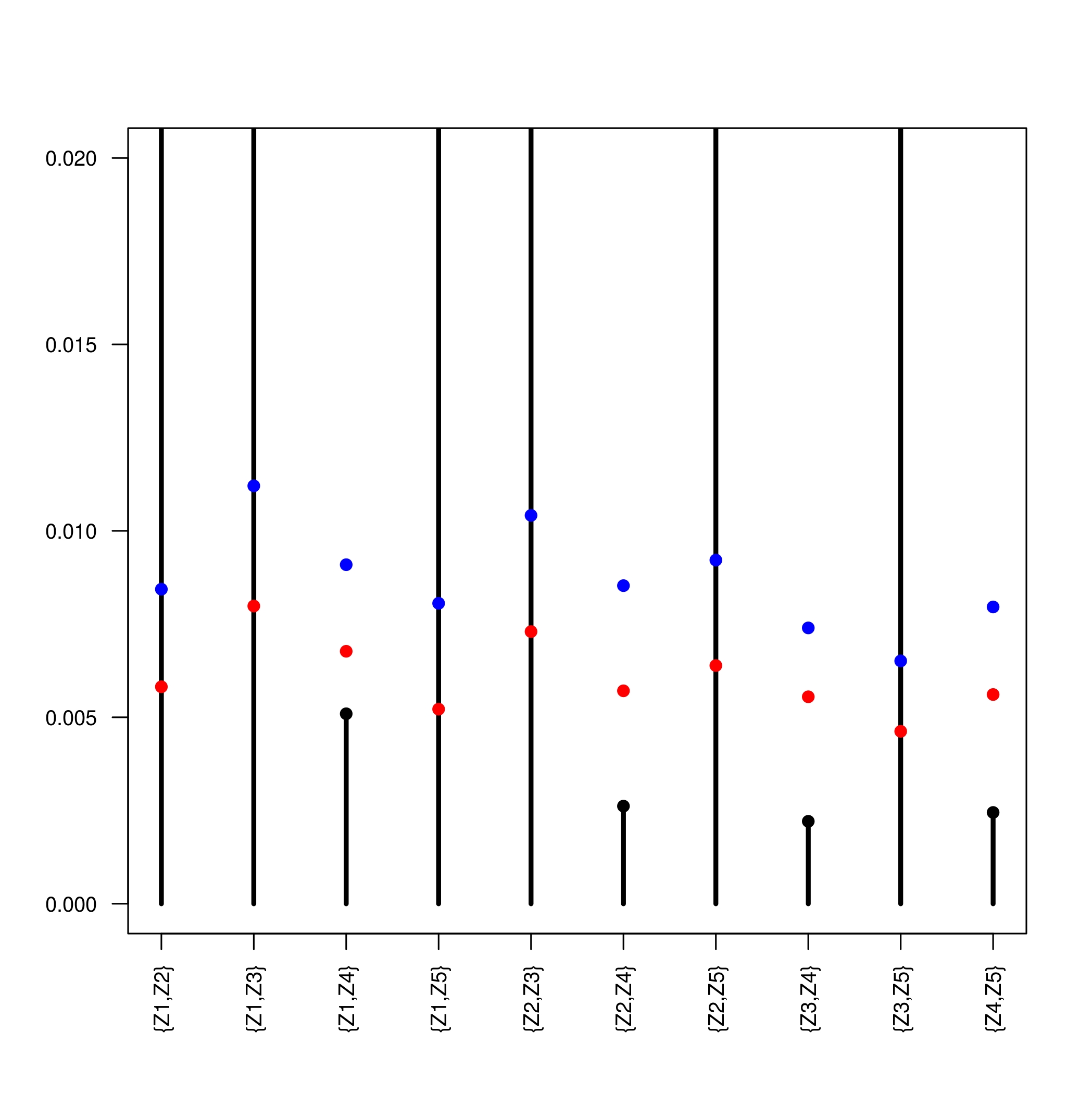
In this subsection we consider the meteorological data given in Table 7.2 of [20]. The data are $46$ observations grouped into $11$ variables defined as follows: $Y_{1}=$“maximum daily air temperature”, $Y_{2}=$“minimum daily air temperature”, $Y_{3}=$“integrated area under daily air temperature curve”, $Y_{4}=$“maximum daily soil temperature”, $Y_{5}=$“minimum daily soil temperature”, $Y_{6}=$“integrated area under daily soil temperature curve”, $Y_{7}=$“maximum daily relative humidity”, $Y_{8}=$“minimum daily relative humidity”, $Y_{9}=$“integrated area under daily humidity curve”, $Y_{10}=$“total wind (in miles per day)” and $Y_{11}=$“evaporation”. We consider the vectors $Z_{1}=(Y_{1},Y_{2},Y_{3})$, $Z_{2}=(Y_{4},Y_{5},Y_{6})$, $Z_{3}=(Y_{7},Y_{8},Y_{9})$ and the variables $Z_{4}=Y_{10}$ and $Z_{5}=Y_{11}$. Taking into account what was seen in the previous section, that there are no important differences between the use of $T_{n}^{(1)}$, $T_{n}^{(2)}$ or $T_{n}^{(\infty)}$ as a test statistic, we apply our independence test between couples of $Z$’s using $T_{n}^{(2,2)}$ as the test statistic. In Table 9 we show the $p$-values of our test in each case. In Figure 4 we show the dependogram of order $2$ of the mutual independence test of the $Z$’s, that is, the critical values at $5\%$ and $10\%$ and the value of our statistic. The approximate $p$-values and critical values were calculated under $m=1000$ replications by a permutation method as has been suggested in [14]. The test concludes that $Z_{1},Z_{2},Z_{3}$ and $Z_{5}$ are pairwise independent, but the wind ($Z_{4}$) does not exhibit any dependence with any of the other variables. On the one hand, these conclusions are equivalent to those obtained in [3]. On the other hand, we observe that in the cases in which the test does not reject $H_{0}$, the difference between the observed and the critical values is very large. The largest observed value, is $0.2887$, reached in the case $Z_{1},Z_{2}$.

Refer to caption
Figure 4: Critical values at $5\%$ (blue), $10\%$ (red) and observed values (black) for the pairwise independence test between the $Z^{\prime}s$ variables.

6.2 Temperature, westbound wind, eastbound wind

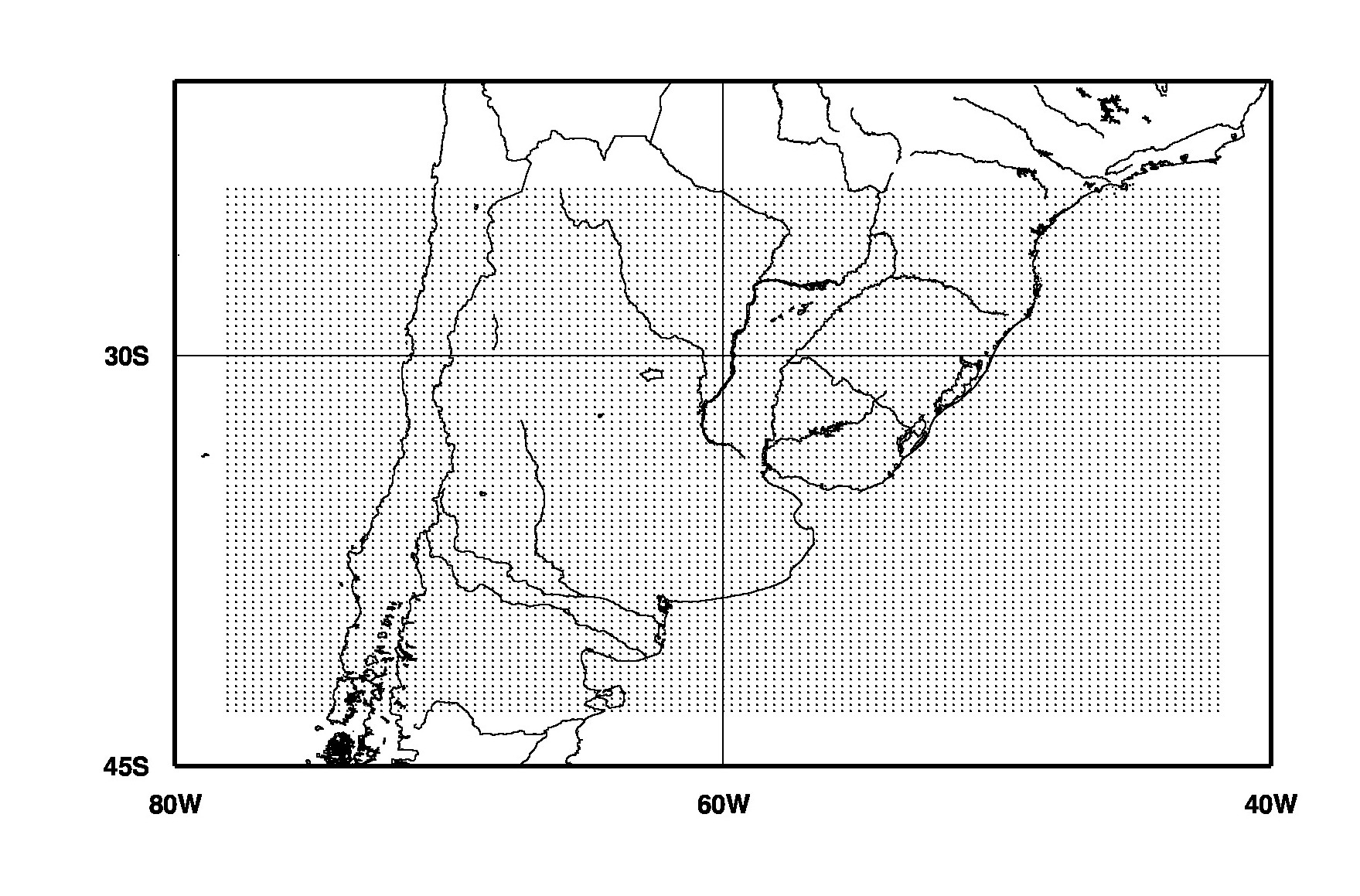
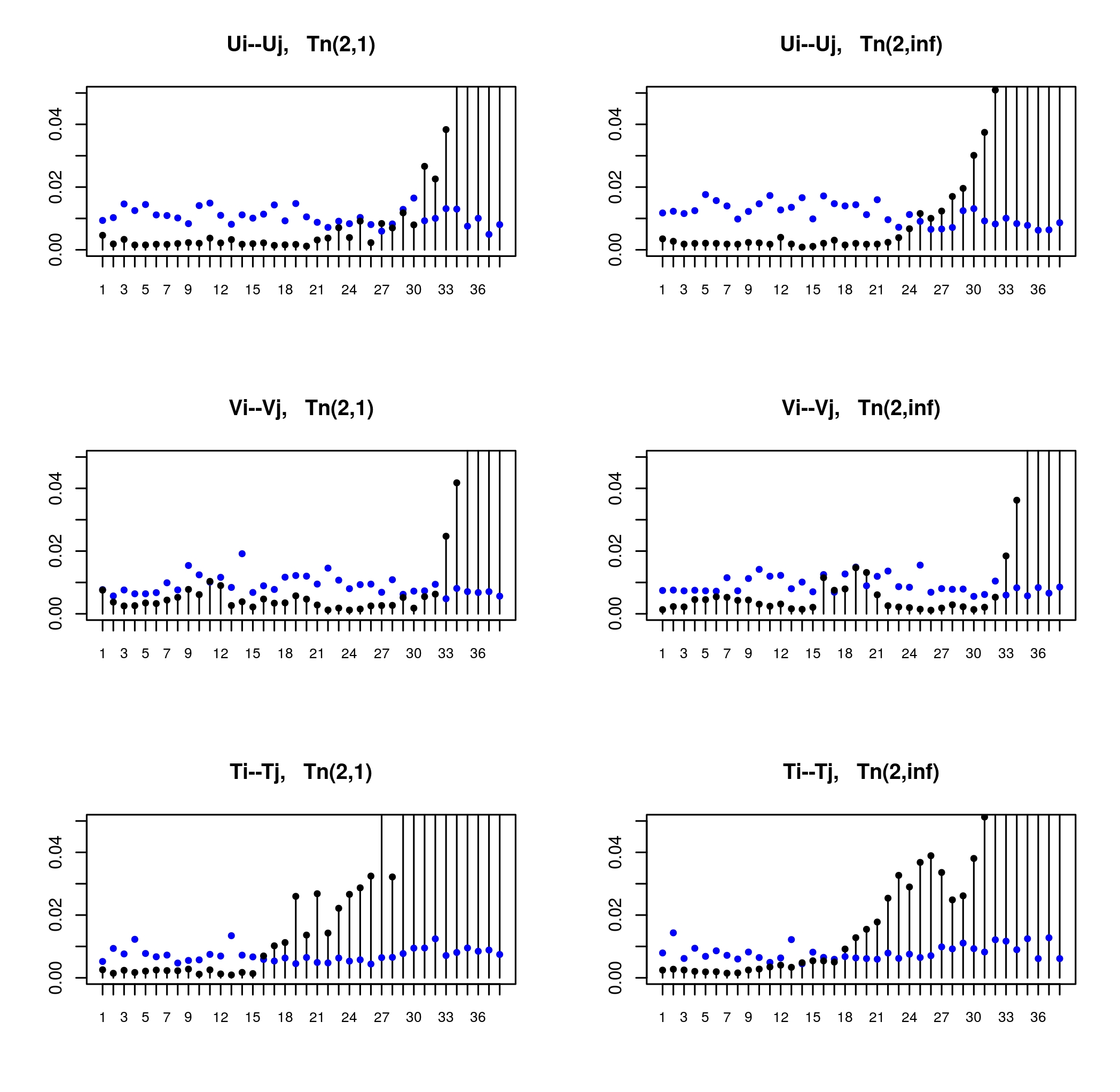
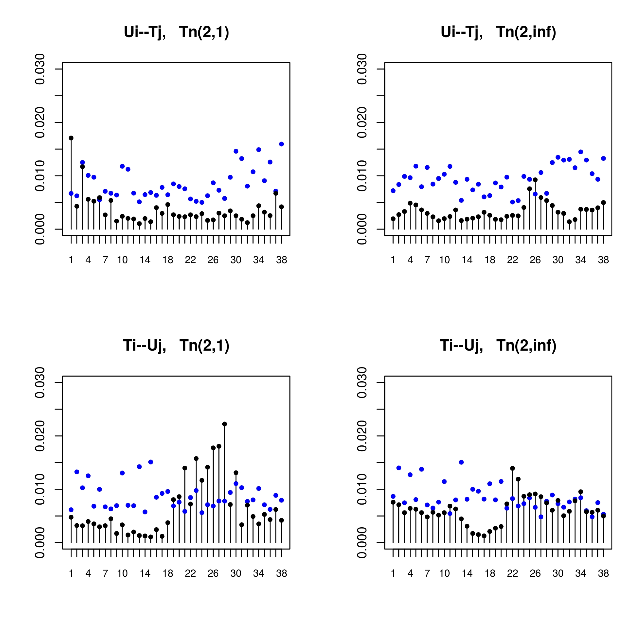
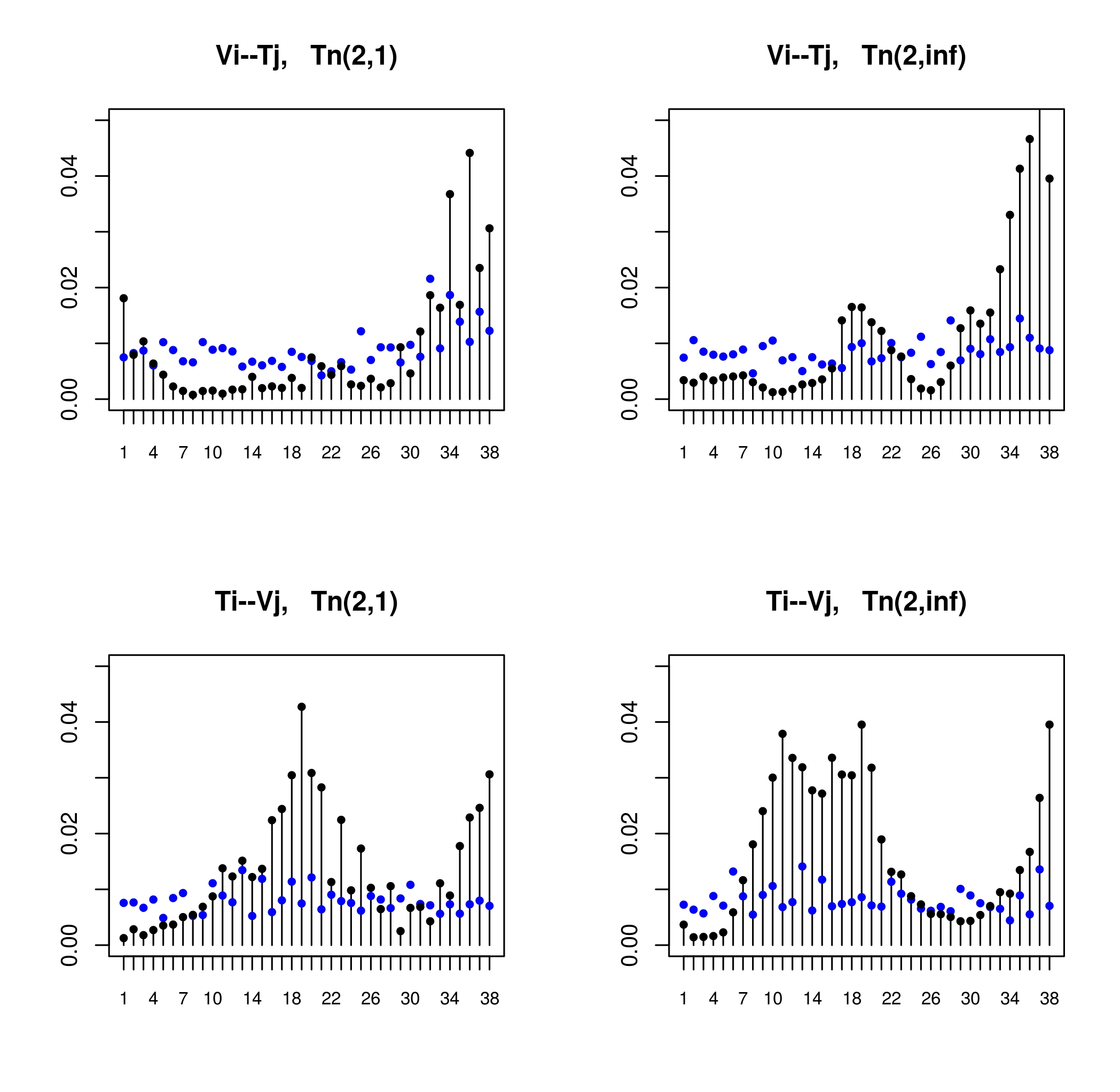
In this subsection we will consider the data set formed by the forecast temperature $(T)$, westbound wind $(U)$ and eastbound wind $(V)$ at $850$ hPa (around $1200$m above sea level) from each day from January 2012 to December 2012. There are a total of $341$ forecasts due to the fact that $25$ data points are missing. The numerical domain is shown in Figure 5 and consists of a total of $117\times 75=8775$ geographical points. The time horizon of the forecasts is $24$ hours, and they are for 0:00 GMT hour of each day. The numerical simulations were obtained using the WRF regional model [21], and the initial and lateral boundary conditions were obtained from the NCEP Global Forecast System, as in [5]. If we consider $(U_{1},V_{1},T_{1}),(U_{2},V_{2},T_{2}),...,(U_{341},V_{341},T_{341})$ where $U_{i},V_{i},T_{i}\in\mathbb{R}^{8775}$ for all $i=1,2,3,...,341$, the $p$-values for the independence test between $U$ and $V$ is equal to zero, and so on for the test between $U$ and $T$, and $V$ and $T$. This is expected because for each geographical point $i$, the variables $U_{i},V_{i}$ and $T_{i}$ are pairwise dependent. Now we consider (for each day) every vector $U\in\mathbb{R}^{8775}$ to be decomposed as $U=(U_{1},U_{2},...,U_{75})$ where $U_{i}\in\mathbb{R}^{117}$. In this form, each $U_{i}$ represents the forecast of the $117$ geographical points at latitude $i$ and can be seen as a discretization of a curve at latitude $i$, ($U(i)$). Here, $i=1$ indicates the southeastern most latitude given in Figure 5 and $i=117$ the northeastern most latitude. We consider the first $30$ forecasts, corresponding to January 2012. In this way, we get a sample of $30$ curves for each latitude $i$, and we will test the mutual independence between $U_{i}$ and $U_{j}$ for $i=1,2,3,...,38$ and $j=76-i$. We decompose $T$ and $V$ analogously. It is to be expected that, at least for small values of $i$, the variables $U_{i}$ and $U_{j}$ would be independent, due to the geographical distance, and the same for the variables $V$ and $T$. In Figures 6, 7, 8 and 9 we show the dependograms for the independence test, using $T_{n}^{(2,1)}$ and $T_{n}^{(2,\infty)}$ statistics, between $U_{i}$ and $U_{76-i}$ for each $i=1,2,...,38$ and the same for the variables $V$, $T$ and the other combinations between $U,V$ and $T$. In Figure 6, similar results between $T_{n}^{(2,1)}$ and $T_{n}^{(2,\infty)}$ are shown. However, in the case of $U_{i}$ and $U_{j}$, $T_{n}^{(2,\infty)}$ detects the dependence in more cases than $T_{n}^{(2,1)}$. Both tests show that when $i$ and $j=76-i$ are close, then the variables $U_{i}$ and $U_{j}$ are dependent. The same occurs with $V_{i}$, $V_{j}$ and $T_{i}$, $T_{j}$. Also the geographical region in which the vectors are dependent is longer for $T$ than for $U$ and $V$. Figure 7 shows that $T_{n}^{(2,1)}$ performs better than $T_{n}^{(2,\infty)}$ because for $i\geq 32$ the test based on $T_{n}^{(2,1)}$ detects a dependence for both cases: $U_{i},V_{j}$ and $V_{i},U_{j}$. Figures 8 and 9 show that the tests based on $T_{n}^{(2,1)}$ and $T_{n}^{(2,\infty)}$ perform similarly. Also, still being geographically close, the vectors $U_{i}$ and $T_{j}$ are independent. However both tests detect a dependence between $T:i$ and $U_{j}$ for $i=21$ to $i=27$ (Figure 8). Figure 9 shows that in most cases, $T_{i}$ and $V_{j}$ are dependent, while for $V_{i}$ and $T_{j}$ the test does not detect a dependence except for the cases in which $i$ and $j$ are close.

Refer to caption
Figure 5: $117\times 75=8775$ geographical points where the daily forecasts are made.
Refer to caption
Figure 6: Comparison between dependograms for $T_{n}^{(2,1)}$ and $T_{n}^{(2,\infty)}$ intra $U,V$ and $T$.
Refer to caption
Figure 7: Comparison between dependograms for $T_{n}^{(2,1)}$ and $T_{n}^{(2,\infty)}$ between $U$ and $V$.
Refer to caption
Figure 8: Comparison between dependograms for $T_{n}^{(2,1)}$ and $T_{n}^{(2,\infty)}$ between $U$ and $T$.
Refer to caption
Figure 9: Comparison between dependograms for $T_{n}^{(2,1)}$ and $T_{n}^{(2,\infty)}$ between $V$ and $T$.

7 Conclusions

In this paper we have proposed several variants to perform the independence test based on recurrence rates. We have shown how to calculate the test statistic in each one of these cases. When $X$ and $Y$ lie in high dimensional spaces, we have shown that the test performs better as the distance function considered goes from the $L^{1}(l^{1})$ distance to the $L^{\infty}(l^{\infty})$ distance in some cases and in the opposite direction in other cases. Therefore, the test statistic using the $L^{1}(l^{1})$ distance and the $L^{\infty}(l^{\infty})$ distances to cover both possibilities can be suggested. From simulations we obtain that in high dimension, our test clearly outperforms the competitors and widely used tests in almost all the alternatives considered. The test was performed on two data sets including small and large sample sizes and we have shown that in both cases the application of the test allows us to obtain interesting conclusions. Taking this together with the simulations presented in [14], we can conclude that the independence test based on recurrence rates has very good performance for random variables, random vectors, and also for random elements lying in high dimensional spaces.

8 Proofs

Proof of Proposition 1.

The proof of this proposition is found in [14]. ∎

Proof of Proposition 2.

We re-order $d\left(X_{i},X_{j}\right)$ with $\left(i,j\right)\in I_{2}^{n}$ in the form $Z_{1},Z_{2},...,Z_{n}.$ Assume that $Z_{1}<Z_{2}<...<Z_{N},$ and we will use $T_{1},T_{2},...,T_{N}$ to denote the values of $d\left(Y_{i},Y_{j}\right)$ using the same indexing. We also write $T_{1}^{\ast},T_{2}^{\ast},...,T_{N}^{\ast}$ for the order statistics of $T^{\prime}s.$

$$\int_{0}^{+\infty}\int_{0}^{+\infty}\left|RR_{n}^{X,Y}\left(r,s\right)-RR_{n}^{X}\left(r\right)RR_{n}^{Y}\left(s\right)\right|g_{1}\left(r\right)g_{2}\left(s\right)drds=$$
$$\frac{1}{N}\int_{0}^{+\infty}g_{2}(s)ds\times$$
$$\int_{0}^{+\infty}\left|\sum_{i\neq j}\mathbf{1}_{\left\{d\left(X_{i},X_{j}\right)<r,\text{ }d\left(Y_{i},Y_{j}\right)<s\right\}}-\frac{1}{N}\sum_{i\neq j}\mathbf{1}_{\left\{d\left(X_{i},X_{j}\right)<r,\right\}}\sum_{h\neq k}\mathbf{1}_{\left\{d\left(Y_{h},Y_{k}\right)<s\right\}}\right|g_{1}\left(r\right)dr=$$
$$\frac{1}{N}\int_{0}^{+\infty}g_{2}(s)ds\int_{0}^{+\infty}\left|\sum_{i=1}^{N}\mathbf{1}_{\left\{Z_{i}<r,\text{ }T_{i}<s\right\}}-\frac{1}{N}\sum_{i=1}^{N}\mathbf{1}_{\left\{Z_{i}<r\right\}}\sum_{j=1}^{N}\mathbf{1}_{\left\{T_{j}<s\right\}}\right|g_{1}\left(r\right)dr.$$ (4)

Observe that

$$\int_{0}^{+\infty}\left|\sum_{i=1}^{N}\mathbf{1}_{\left\{Z_{i}<r,\text{ }T_{i}<s\right\}}-\frac{1}{N}\sum_{i=1}^{N}\mathbf{1}_{\left\{Z_{i}<r\right\}}\sum_{j=1}^{N}\mathbf{1}_{\left\{T_{j}<s\right\}}\right|g_{1}\left(r\right)dr=$$
$$\sum_{h=1}^{N-1}\int_{Z_{h}}^{Z_{h+1}}\left|\sum_{i=1}^{h}\mathbf{1}_{\left\{T_{i}<s\right\}}-\frac{h}{N}\sum_{j=1}^{N}\mathbf{1}_{\left\{T_{j}<s\right\}}\right|g_{1}\left(r\right)dr=$$
$$\sum_{h=1}^{N-1}\left|\sum_{i=1}^{h}\mathbf{1}_{\left\{T_{i}<s\right\}}-\frac{h}{N}\sum_{j=1}^{N}\mathbf{1}_{\left\{T_{j}<s\right\}}\right|\left(G_{1}\left(Z_{h+1}\right)-G_{1}\left(Z_{h}\right)\right).$$

Then, (4) is equal to

$$\frac{1}{N}\sum_{h=1}^{N-1}\left(G_{1}\left(Z_{h+1}\right)-G_{1}\left(Z_{h}\right)\right)\int_{0}^{+\infty}\left|\sum_{i=1}^{h}\mathbf{1}_{\left\{T_{i}<s\right\}}-\frac{h}{N}\sum_{j=1}^{N}\mathbf{1}_{\left\{T_{j}<s\right\}}\right|g_{2}(s)ds=$$
$$\frac{1}{N}\sum_{h=1}^{N-1}\left(G_{1}\left(Z_{h+1}\right)-G_{1}\left(Z_{h}\right)\right)\sum_{j=1}^{N-1}\int_{T_{j}^{\ast}}^{T_{j+1}^{\ast}}\left|\sum_{i=1}^{h}\mathbf{1}_{\left\{T_{i}<s\right\}}-\frac{h}{N}\sum_{j=1}^{N}\mathbf{1}_{\left\{T_{j}<s\right\}}\right|g_{2}(s)ds=$$
$$\frac{1}{N}\sum_{h=1}^{N-1}\left(G_{1}\left(Z_{h+1}\right)-G_{1}\left(Z_{h}\right)\right)\sum_{j=1}^{N-1}\int_{T_{j}^{\ast}}^{T_{j+1}^{\ast}}\left|c(h,j)-\frac{jh}{N}\right|g_{2}(s)ds=$$
$$\frac{1}{N}\sum_{h,j=1}^{N-1}\left(G_{1}\left(Z_{h+1}\right)-G_{1}\left(Z_{h}\right)\right)\left(G_{2}\left(T_{j+1}^{\ast}\right)-G_{2}\left(T_{j}^{\ast}\right)\right)\left|c(h,j)-\frac{jh}{N}\right|,$$

where $c(h,j)=\sum_{i=1}^{h}\mathbf{1}_{\left\{T_{i}<T_{j+1}^{\ast}\right\}}$ is the number of elements of the vector $\left(T_{1},T_{2},...,T_{h}\right)$ that are less than $T_{j+1}^{\ast}$ for $h,j=1,2,3,...,N-1.$ Thus,

$$T_{n}^{\left(1\right)}=\frac{\sqrt{n}}{N}\sum_{h,j=1}^{N-1}\left(G_{1}\left(Z_{h+1}\right)-G_{1}\left(Z_{h}\right)\right)\left(G_{2}\left(T_{j+1}^{\ast}\right)-G_{2}\left(T_{j}^{\ast}\right)\right)\left|c(h,j)-\frac{jh}{N}\right|.$$

Proof of Proposition 3.

In accordance with Steps 1 and 2, we put $N=n(n-1)$ and re-order $\left\{d\left(X_{i},X_{j}\right)\right\}_{i\neq j}$ as $Z_{1},Z_{2},...,Z_{N}$ such that $Z_{1}<Z_{2}<...<Z_{N}$ and $\left\{d\left(Y_{i},Y_{j}\right)\right\}_{i\neq j}$ as $T_{1},T_{2},...,T_{N}$ maintaining the same indexing as $Z^{\prime}s$ (that is, if $d\left(X_{i},X_{j}\right)=Z_{h}$, then $d\left(Y_{i},Y_{j}\right)=T_{h}$). Observe that, to compute $T_{n}^{(\infty)}(r,s)$ for all $r,s>0$ it is enough to compute $T_{n}^{(\infty)}(Z_{i},T_{j}^{*})$ for every $i,j=1,2,...,N.$ Then, the result follows immediately from Steps 4 and 5.

Acknowledgements We would like to express our gratitude to Leonardo Moreno for his explanations about the independence test based on random projections and for giving us the R code to use it, and to Gabriel Cazes for giving us the data sets and the map of Figure 5.

References

  • [1] Arratia, A., Cabaña, A. & Cabaña, E., (2016). A construction of Continuous time ARMA models by iterations of Ornstein-Uhlenbeck process, SORT Vol 40 (2) 267-302.
  • [2] R. Beran, M. Bilodeau, P. Lafaye de Micheaux, Nonparametric tests of independence between random vectors, Journal of Multivariate Analysis, 98 (9) (2007)1805–1824.
  • [3] Bilodeau, M. & Getsop, A., (2017). Test of Mutual or Serial Independence of Random Vectors with Applications, Journal of Machine Learning Vol 18, 1-40.
  • [4] N. Blomqvist, On a measure of dependence between two random variables, The Annals of Mathematical Statistics, (1950) 593-600.
  • [5] Cazes Boezio G., Ortelli, S., (2018). Minimum-cost numerical prediction system for wind power in Uruguay, with an assessment of the diurnal and seasonal cycles of its quality. Ciencia e Natura, Vol 40, 206 - 210.
  • [6] Fraiman, R., Moreno, L. & Vallejo, S. (2017) Some hypothesis tests based on random projection. Computational Statistics. 32: 1165-1189.
  • [7] F. Galton, Co-relations and their measurement, chiefly from anthropometric data, Proceedings of the Royal Society of London, 45 (273-279) (1888) 135–145.
  • [8] G. Genest, B. Rémillard, Test of independence and randomness based on the empirical copula process. Test, 13 (2) (2004) 335-369.
  • [9] Gretton, A., K. Fukumizu, C. H. Teo, L. Song, B. Schölkopf & A. J. Smola (2007). A kernel statistical test of independence. In Advances in Neural Information Processing Systems. 585-592.
  • [10] A. Gretton, O. Bousquet, A. Smola, B. Schölkopf, Measuring statistical dependence with Hilbert-Schmidts norms, International Conference on algorithmic learning theory, (2005) 63-77.
  • [11] W. Hoeffding, The strong law of large numbers for $U$-statistics. Available at:
    http://www.lib.ncsu.edu/resolver/1840.4/2128 (1961).
  • [12] J. Kalemkerian, Parameter Estimation for Discretely Observed Fractional Iterated Ornstein–Uhlenbeck Processes. (2020). arXiv:2004.10369
  • [13] J. Kalemkerian, J. R. León, Fractional iterated Ornstein-Uhlenbeck Processes, ALEA A Lat. Am. J. Probab. Math. Stat. (2019) 16 1105–1128.
  • [14] Kalemkerian, J. & Fernández, D. (2020). An independence test based on recurrence rates. Journal of Multivariate Analysis. https://doi.org/10.1016/j.jmva.2020.104624
  • [15] Kalemkerian, J. & Fernández, D. (2019). Implementación del test de independencia basado en porcentaje de recurrencias para series de tiempo. https://www.bcu.gub.uy/Comunicaciones/Jornadas%20de%20Economa/FE
    RNANDEZ_DIEGO_2019_2.pdf
  • [16] M. G. Kendall, A new measure of rank correlation, Biometrika, 30(1/2) (1938) 81–93.
  • [17] I. Kojadinovic, M. Holmes, Tests of independence among continuous random vectors based on cramér-von mises functional of the empirical copula process, Journal of Multivariate Analysis, 100 (6) (2009) 1137-1154.
  • [18] N. Marwan, A Historical Review of Recurrence Plots, European Physical Journal Special Topics, 164 (2008) 3-12.
  • [19] K. Pearson, Mathematical contributions to the theory of evolution on a form of spurious correlation which may arise when indices are used in the measurement of organs, Proceedings of the Royal Society of London. 60 (359-367) (1898) 489–498.
  • [20] Rencher, A. C. (1995). Methods of Multivariate Analysis. Wiley Series in Probability and Mathematical Statistics. John Wiley & Sons, New York, 1995.
  • [21] Skamarock, W.C. and list of coauthors. A description of the Advanced Research WRF version 3. NCAR Tech Note NCAR/TN-475+STR, 113 pp. www.mmm.ucar.edu/wrf/users/docs/arw_v3.pdf.
  • [22] C. Spearman, The proof and measurement of association between two things, The American journal of psychology, 15 (1) (1904) 72–101.
  • [23] Székely G.J & Rizzo M.L. (2013) The distance correlation t-test of independence in high dimension. Journal of Multivariate Analysis 117:193–213.
  • [24] G. J. Székely, M.L. Rizzo, N.K. Bakirov, Measuring and testing dependence by correlation of distances, The Annals of Statistics. 35 (6) (2007) 2769– 2794.
  • [25] G.J. Székely, M.L Rizzo, Brownian distance covariance, The annals of applied statistics, 3(4) (2009) 1236–1265.
  • [26] S. Wilks, On the independence of $k$ sets of normality distributed statistical variables, Econometrica, Journal of the Econometric Society, (1935) 309-326.