A note on optimal designs for estimating the slope of a polynomial regression

Abstract

In this note we consider the optimal design problem for estimating the slope of a polynomial regression with no intercept at a given point, say $z$. In contrast to previous work, which considers symmetric design spaces we investigate the model on the interval $[0,a]$ and characterize those values of $z$, where an explicit solution of the optimal design is possible.

AMS subject classification: 62K05

Keywords and phrases: polynomial regression, slope estimation, $c$-optimal designs

1 Introduction

Consider the common polynomial regression model of degree $n$ with no intercept

$$Y_{i}=f^{\top}(x_{i})\theta+\varepsilon_{i}=(x_{i},x_{i}^{2},\dots,x_{i}^{n})^{\top}\theta+\varepsilon_{i},\qquad i=1,\ldots,N,$$ (1.1)

where $\varepsilon_{1},\dots,\varepsilon_{N}$ denote independent random variables with $\mathbb{E}[\varepsilon_{i}]=0;$ ${\rm Var}(\varepsilon_{i})=\sigma^{2}>0$, $\theta=(\theta_{1},\ldots,\theta_{n})^{\top}\in\mathbb{R}^{n}$ is a vector of unknown parameters and the explanatory variables $x_{1},\ldots,x_{N}$ vary in the interval $[0,a]$ for some $a>0$. An approximate optimal design [in the sense of Kiefer, (1974)] minimizes an appropriate function of the (asymptotic) covariance matrix of the statistic $\sqrt{N}\hat{\theta}$, where the $\hat{\theta}$ denotes the least squares estimate of the parameter $\theta$ in the regression model (1.1) [see Silvey, (1980) or Pukelsheim, (2006)].

In a recent paper Dette et al., (2020) considered model (1.1) on the symmetric interval $[-1,1]$ and determined explicitly the approximate optimal design for estimating the derivative of the regression function

$${d\over dx}f^{\top}(x)\theta\Big{|}_{x=z}=\sum_{j=1}^{n}j\theta_{j}z^{j-1}$$

at the point $z$, which minimizes the variance of the best linear unbiased estimate of $\sum_{j=1}^{n}j\theta_{j}z^{j-1}$. The corresponding optimality criterion is a special case of the well known $c$-optimality criterion [see, for example, Elfving, (1952); Studden, (1968) or Pukelsheim, (2006), Chapter 2].

In practice, however, polynomial regression models with no intercept are usually used on a positive interval, where $x$ corresponds, for example, to speed, concentration or time, and the response at the initial point $x=0$ is [see, for example, Huang et al., (1995); Li et al., (2005)]. Therefore the goal of this note is to provide some optimal designs for estimating the slope of polynomial regression model with no intercept in the case where the design space is given by the interval $[0,a]$. In Section 2 we introduce the basic optimal design problem and review a geometric characterization of $c$-optimal designs. The main result can be found in Section 3 where the optimal designs for estimating the slope at the point in a polynomial regression model with no intercept are determined explicitly and the theory is illustrated by several examples.

2 $c$-optimal designs

Consider the regression model (1.1) on the interval $[0,a]$. Following Kiefer, (1974) we call a discrete probability measure

$$\xi=\begin{pmatrix}x_{1}&\cdots&x_{m}\\ \omega_{1}&\cdots&\omega_{m}\end{pmatrix}$$

with support points $x_{1},\ldots,x_{m}\in[0,a]$ and weights $\omega_{1},\ldots,\omega_{m}$ an approximate design (on the interval $[0,a]$). If $N$ observations can be taken this means that the quantities $N\omega_{i}$ are rounded to integers, say $n_{i}$, with $\sum_{i=1}^{m}n_{i}=N$ and $n_{i}$ observations are taken at each experimental condition ${x_{i}}$ ($i=1,\ldots,m$). For an approximate design $\xi$ we denote by

$$M(\xi)=\int_{[0,a]}f(x)f^{\top}(x)\xi(dx)$$

its information matrix in the model (1.1), where $f(x)=(x,\ldots,x^{n})^{\top}$ is the vector regression functions. The covariance matrix of the least squares estimate for the parameter $\theta$, say $\hat{\theta}$, can be approximated (if $N\to\infty$, $n_{i}/N\to\omega_{i}$) by $\sigma^{2}/NM^{-1}(\xi)$ and an optimal design minimizes an appropriate real valued function of the matrix $M^{-1}(\xi)$. In this paper we are interested in designs minimizimng the asymptotic variance of the best linear unbiased estimate $c^{\top}\hat{\theta}$ of the linear combination $c^{\top}\theta$ for a given vector $c\in\mathbb{R}^{n}$. To be precise, we call a design $\xi$ $c$-optimal in the regression model (1.1), if it minimizes the function

$$\Phi(\xi)=\begin{cases}c^{\top}M^{-}(\xi)c,\text{ if there exists a vector}v\in\mathbb{R}^{d}\text{ such that }c=M(\xi)v;\\ \infty,\text{ otherwise, }\end{cases}$$

where $M^{-}(\xi)$ is a generalized inverse for the matrix $M(\xi)$. In the first case the design $\xi$ is called admissible for estimating the linear combination $c^{\top}\theta$ in the regression model (1.1) and the value of the quadratic form does not depend on the choice of the generalized inverse [see Pukelsheim, (2006)]. The choice $c=f^{\prime}(z)=(1,2z,\ldots,nz^{n-1})^{\top}$ for some $z$ corresponds to the minimization of the variance of the best unbiased prediction of the derivative of the regression function $\theta^{\top}f(x)$ at the point $z$. The optimal design is called optimal design for estimating derivative at the point $z$ in this case.

A useful tool for the determination of $c$-optimal designs is a geometric characterization of the $c$-optimal design and which is called Elfving’s theorem in the literature [see Elfving, (1952)]. We formulate it here in a slightly different form, which can be directly used to check optimality of a given design [see Dette et al., (2004) for details].

Theorem 2.1

An admissible design $\xi^{*}$ for estimating the linear combination $c^{\top}\theta$ with support points $x_{1},x_{2},\ldots,x_{m}\in{\cal X}=[0,a]$ and weights $\omega_{1},\omega_{2},\ldots,\omega_{m}$ is $c$-optimal if and only if there exists a vector $p\in\mathbb{R}^{n}$ and a constant $h$ such that the following conditions are satisfied:

• $|p^{\top}f(x)|\leq 1$ for all $x\in\mathcal{X}$;

• $|p^{\top}f(x_{i})|=1$ for all $i=1,2,\ldots,m$ ;

• $c=h\sum_{i=1}^{m}f(x_{i})\omega_{i}p^{\top}f(x_{i})$.

Moreover, in this case we have $c^{\top}M^{-}(\xi^{*})c=h^{2}$ and the function $p^{\top}f(x)$ is called extremal polynomial.

3 Optimal designs for estimating the slope

For the linear model through the origin (that is $n=1$) it is easy to see using Elfving’s theorem that the optimal design for estimating the slope is unique and puts all mass at the point $a$ (independently of the point $z$). However, in the case $n>1$ the situation is more complicated. By Theorem 2.1 it follows that the support points of the optimal design are extremal points of a polynomial of the form $p^{\top}f(x)=\sum_{i=1}^{n}p_{i}x^{i}$. In fact it is possible to identify a candidate for this optimal polynomial explicitly. For this purpose let

$$T_{n}(x)=\cos(n\arccos(x))$$

denote the $n$th Chebyshev polynomial of the first kind [see Szegö, (1975)] and consider the polynomial

$$S_{n}(x)=T_{n}\Bigl{(}\frac{x}{a}(1+\cos\frac{\pi}{2n})-\cos\frac{\pi}{2n}\Bigr{)}.$$ (2.1)

It is easy to see that $S_{n}(x)$ has exactly $n$ extremal points $s_{1}<s_{2}<\cdots<s_{n}$ on the interval $[0,a]$, which are given by

$$s_{i}=a\cdot\frac{\cos\frac{(i-1)\pi}{n}+\cos\frac{\pi}{2n}}{1+\cos\frac{\pi}{2n}},~{}~{}i=1,2,\dots,n.$$ (2.2)

For the statement of our main result we define $\bar{L}_{1},\ldots,\bar{L}_{n}$ as the Lagrange basis interpolation polynomials without intercept corresponding to the nodes $s_{1},\ldots,s_{n}$, that is

$$\bar{L}_{i}(z)=\dfrac{z\prod_{j\neq i}(z-s_{j})}{s_{i}\prod_{j\neq i}(s_{i}-s_{j})},$$ (2.3)

and denote by $\bar{L}_{i}^{\prime}$ the derivative of $\bar{L}_{i}$ ($i=1,\ldots,n$).

Theorem 3.1

Consider the polynomial regression model of degree $n>1$ with no intercept on the interval $[0,a]$. The optimal design $\xi^{*}(z)$ for estimating the slope of this model at the point $z$ is supported at the points $s_{1},\ldots,s_{n}$ defined in (2.2) if and only if

$$z\in\bigcup_{i=1}^{n}(\omega_{1,i-1},\omega_{n,i}),$$

where $-\omega_{1,0}=\omega_{n,n}=\infty$ and $\omega_{i,k}$ is $k$-th root of the function

$$\omega_{i}(z)=\dfrac{|\bar{L}^{\prime}_{i}(z)|}{\sum_{j=1}^{n}|\bar{L}^{\prime}_{j}(z)|}~{},~{}i=1,\ldots,n,$$ (2.4)

$k=1,\ldots,n-1,j=1,\ldots,n.$ Moreover, in this case the weight of the design $\xi^{*}(z)$ at $s_{i}$ is given by $\omega_{i}(z)$ ($i=1\ldots,n$).

To prove this Theorem we use the following Lemma. The proof can be found in Sahm, (1998) or in Dette et al., (2020).

Lemma 3.2

Let $P_{1}(x)$ and $P_{2}(x)$ be polynomials of degree $n$ with $n$ distinct roots $t_{(1,1)}<t_{(1,2)}<\ldots<t_{(1,n)}$ and $t_{(2,1)}<t_{(2,2)}<\ldots<t_{(2,n)}$, respectively. Assume that the roots are interlacing in the following sense:

$$t_{(1,1)}\leq t_{(2,1)}<t_{(1,2)}\leq t_{(2,2)}<\ldots<t_{{(1,n)}}\leq t_{{(2,n)}}~{},$$

where at least one of the inequalities $t_{{(\ell,1)}}\leq t_{{(\ell,2)}}$ ($\ell=1,\ldots n$) is strict. Then the roots $v_{(1,1)}\leq v_{(1,2)}\leq\ldots\leq v_{(1,n-1)}$ and $v_{(2,1)}\leq v_{(2,2)}\leq\ldots\leq v_{(2,n-1)}$ of the derivatives $P_{1}^{\prime}(x)$ and $P_{2}^{\prime}(x)$ are strictly interlacing, that is

$$v_{(1,1)}<v_{(2,1)}<\ldots<v_{(1,n-1)}<v_{(2,n-1)}.$$

Proof of Theorem 3.1.

We will check the optimality of the design $\xi^{*}(z)$ by an application of Theorem 2.1. Note, that the polynomial $S_{n}(z)$ defined in (2.1) obviously satisfies to conditions (1) and (2) of this theorem.

It now remains to characterize those values of $z$ such that the system of equations defined by condition (3) in Theorem 2.1 admits a solution with nonnegative weights $\omega_{i}$ satisfying $\sum_{i=1}^{m}\omega_{i}=1$. Note that condition (3) in Theorem 2.1 can be rewritten in the form

$$c=f^{\prime}(z)=(1,z,\ldots,nz^{n-1})^{\top}=hF\beta,$$ (2.5)

where

$$F=((s_{j})^{i})_{i,j=1}^{n}=(f(s_{1}),\ldots,f(s_{n}))\in\mathbb{R}^{n\times n}\ \hbox{and}\ \ \beta_{i}=\omega_{i}(p^{\top}f(s_{i}))$$

In order to investigate the system of equations defined by (2.5) note that the identity $F^{-1}F=I_{n}$ (here $I_{n}$ is the identity matrix) implies

$$e_{i}^{\top}F^{-1}f(s_{j})=\delta_{ij}~{}~{}~{}(i,j=1,\ldots,n),$$

where $\delta_{ij}$ is the Kroneker symbol and $e_{i}=(0,\ldots,0,1,0,\ldots,0)^{\top}\in\mathbb{R}^{n}$ the $i$th unit vector. As these equations characterize the $i$th Lagrange basis interpolation polynomial $\bar{L}_{i}(z)=a_{i}^{T}f(z)$ with nodes $s_{1},\ldots,s_{n}$ we have

$$e_{i}^{\top}F^{-1}f(z)=\bar{L}_{i}(z),\;i=1,\ldots,n.$$

Differentiating both sides of the equation with respect to $z$ yields

$$e_{i}^{\top}F^{-1}f^{\prime}(z)=\bar{L}^{\prime}_{i}(z),\;i=1,\ldots,n,$$

or equivalently

$$F^{-1}f^{\prime}(z)=(\bar{L}^{\prime}_{1}(z),\ldots,\bar{L}^{\prime}_{n}(z))^{\top}.$$

Therefore we obtain for the solution of (2.5)

$$h\beta=(\bar{L}^{\prime}_{1}(z),\ldots,\bar{L}^{\prime}_{n}(z))^{\top}$$

or equivalently (since ${\beta}_{i}=\omega_{i}(p^{\top}f(s_{i}))$)

$$h\beta_{i}=h\omega_{i}(-1)^{n-i}=\bar{L}^{\prime}_{i}(z)~{},~{}~{}i=1,\ldots,n.$$ (2.6)

Consequently applying Lemma 3.2 to the pairs of polynomials $\bar{L}_{i}(z),\bar{L}_{i+1}(z)$ from (2.3) $i=1,\dots,n-1$ we obtain that the roots of functions $\bar{L}^{\prime}_{i}(z)$ are strictly interlacing, that is

$$\omega_{(n,1)}<\ldots<\omega_{(1,1)}<\omega_{(n,2)}<\ldots<\omega_{(1,2)}<\ldots<\omega_{(1,n-2)}<\omega_{(n,n-1)}<\ldots<\omega_{(1,n-1)}.$$

This immediately implies that each of the functions $\bar{L}^{\prime}_{i}(z)$ has only one root in the intervals $[\omega_{(n,i)},\omega_{(1,i)}]$ and has no roots in the intervals $A_{1},\ldots,A_{n}$, where the set $A_{i}$ is defined by $A_{i}=(\omega_{1,i-1},\omega_{n,i})$, $i=1,\dots,n$. Moreover, for $z\in A_{n}$ we have

$$\mbox{sign}((-1)^{n-i}\bar{L}^{\prime}_{i}(z))=1~{},~{}~{}i=1,\ldots,n$$

(since $\mbox{sign}(\bar{L}^{\prime}_{i}(z))=(-1)^{n-i}$), and for $z\in A_{j}$

$$\mbox{sign}((-1)^{n-i}\bar{L}^{\prime}_{i}(z))=(-1)^{n+j}~{},~{}~{}i,j=1,\ldots,n.$$

This implies that

$$|\bar{L}^{\prime}_{i}(z)|=(-1)^{n+j}(-1)^{n-i}\bar{L}^{\prime}_{i}(z)~{}~{}(i,j=1,\ldots,n)$$

for $z\in A_{j}$.

The proof is now completed observing (2.6), which implies that for $z\in A_{j},$ the weights are given by

$$\omega_{i}(z)={(-1)^{n-i}\bar{L}^{\prime}_{i}(z)\over h}={(-1)^{n+j}|\bar{L}^{\prime}_{i}(z)|\over h}~{}~{}(i=1,\ldots,n)$$

with $h=(-1)^{n+j}\sum_{i=1}^{n}|\bar{L}^{\prime}_{i}(z)|$. $\Box$

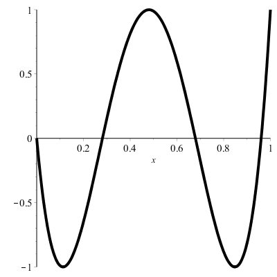
Figure 1: The extremal polynomial $S_{4}(x)$ on the interval $[0,1]$ ($a=1$).

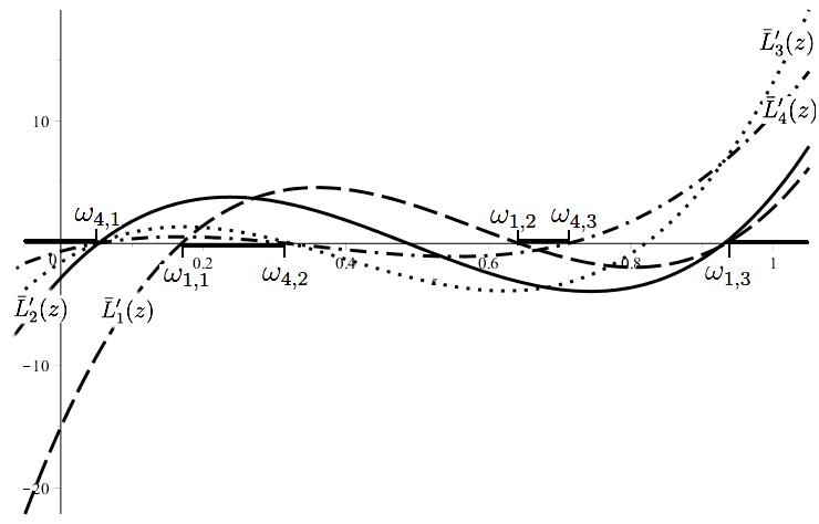
Figure 2: The functions $\bar{L}_{i}^{\prime}(z),$ $z\in\mathbb{R}$ for $i=1,2,3,4$ ($n=4,\ a=1$).

Example 3.3

In this example we illustrate potential applications of Theorem 3.1 determining optimal designs for estimating the slope of a polynomial regression with no intercept on the interval $[0,1]$.

We start with the case of a quadratic regression model, that is $n=2$. Here the extremal points in (2.2) are given by $s_{1}=\sqrt{2}-1,s_{2}=1$ and the derivatives of the polynomials in (2.3) are calculated as

$$\bar{L}_{1}^{\prime}(z) =-\frac{4+3\sqrt{2}}{2}(2z-1)~{},~{}\bar{L}_{2}^{\prime}(z)=-\frac{2+\sqrt{2}}{2}(-2z+\sqrt{2}-1).$$

The corresponding roots of the functions (2.4) are obtained as

$$\omega_{1,1}=\frac{1}{2}~{},~{}\omega_{2,1}=\frac{1}{2}(1-\sqrt{2})$$

and the optimal design for estimating the slope of the polynomial regression without intercept is supported at points $\sqrt{2}-1,1$ if and only if

$$z\in\Big{(}-\infty,\frac{1}{2}(1-\sqrt{2})\Big{)}\cup\Big{(}\frac{1}{2},\infty\Big{)}$$

As a second example we consider the cubic regression model with no intercept, that is $n=3$. In this case the extremal points of the polynomial $S_{3}(x)$ are $s_{1}=3\sqrt{3}-5,$ $s_{2}=\sqrt{3}-1$, $s_{3}=1$ and the derivatives of the Lagrange interpolation polynomials in (2.3) are given by

$$\bar{L}_{1}^{\prime}(z) =35.490z^{2}-40.981z+8.6607~{},~{}\bar{L}_{2}^{\prime}(z)=-28.548z^{2}+22.767z-1.8680$$

$$\bar{L}_{3}^{\prime}(z) =13.933z^{2}-8.6240z+.66745,$$

The roots of the roots of the functions (2.4) are obtained as

$$\omega_{1,1}=0.2785~{},~{}\omega_{2,1}=0.0935~{},~{}\omega_{3,1}=0.090~{},~{}\omega_{1,2}=0.8758~{},~{}\omega_{2,2}=0.7045~{},~{}\omega_{3,2}=0.528$$

By Theorem 3.1 the optimal design for estimating the slope of the polynomial regression without intercept at the point $z$ is supported at the points $\{3\sqrt{3}-5,\sqrt{3}-1,1\}$ if and only if

$$z\in(-\infty,0.090)\cup(0.2785,0.528)\cup(0.8758,\infty)$$

Finally we consider model (1.1) with $n=4$, where the extremal polynomial $S_{4}(x)$ is displayed in Figure 1. The corresponding extremal points are given by $s_{1}=0.1127$, $s_{2}=0.4802,$, $s_{3}=0.8477$ and $s_{1}=1$. The derivatives of the polynomials in (2.3) are calculated as

$$\bar{L}_{1}^{\prime}(z) =-148.08z^{3}+258.55z^{2}-128.47z+15.072,$$

$$\bar{L}_{2}^{\prime}(z) =118.63z^{3}-174.42z^{2}+62.631z-2.8327$$

$$\bar{L}_{3}^{\prime}(z) =-114.72z^{3}+137.04z^{2}-37.110z+1.5517,$$

$$\bar{L}_{4}^{\prime}(z) =56.968z^{3}-61.552z^{2}+15.858z-0.65327$$

and displayed in Figure 2. The roots of the functions (2.4) are given by

$$\omega_{1,1}=0.1696~{},~{}\omega_{2,1}=0.05268~{},~{}\omega_{3,1}=0.05102~{},~{}\omega_{4,1}=0.05071,$$

$$\omega_{1,2}=0.6432~{},~{}\omega_{2,2}=0.4872~{},~{}\omega_{3,2}=0.3232~{},~{}\omega_{4,2}=0.3175,$$

$$\omega_{1,3}=0.9332~{},~{}\omega_{2,3}=0.9305~{},~{}\omega_{3,3}=0.8205~{},~{}\omega_{4,3}=0.7123.$$

Therefore, by Theorem 3.1 the optimal design for estimating the slope of the polynomial regression without intercept at the point $z$ is supported at the points $0.1127,0.4802,0.8477,1$ if and only if

$$z\in(-\infty,0.05071)\cup(0.1696,0.3175)\cup(0.6432,0.7123)\cup(0.9332,\infty)$$

Acknowledgements

The work of H. Dette has been supported in part by the German Research Foundation, DFG (SFB 823, Teilprojekt C2, Germany’s Excellence Strategy - EXC 2092 CASA - 390781972). The work of Viatcheslav Melas and Petr Shpilev was partly supported by Russian Foundation for Basic Research (project no. 20-01-00096).

References

- Dette et al., (2020) Dette, H., Melas, V. B., and Shpilev, P. (2020). Some explicit solutions of c-optimal design problems for polynomial regression with no intercept. Accepted for publication by Annals of the Institute of Statistical Mathematics. https://doi.org/10.1007/s10463-019-00736-0.
- Dette et al., (2004) Dette, H., Melas, V. B., and Pepelyshev, A. (2004). Optimal designs for estimating individual coefficients in polynomial regression - a functional approach. Journal of Statistical Planning and Inference, 118(1):201 – 219.
- Elfving, (1952) Elfving, G. (1952). Optimal allocation in linear regression theory. The Annals of Mathematical Statistics, 23:255–262.
- Huang et al., (1995) Huang, M.-N. L., Chang, F.-C., and K., W. W. (1995). -optimal designs for polynomial regression without an intercept. Statistica Sinica, 5(2):441–458.
- Kiefer, (1974) Kiefer, J. (1974). General Equivalence Theory for Optimum Designs (Approximate Theory). The Annals of Statistics, 2(5):849–879.
- Li et al., (2005) Li, K.-H., Lau, T.-S., and Zhang, C. (2005). A note on -optimal designs for models with and without an intercept. Statistical Papers., 46(3):451–458.
- Pukelsheim, (2006) Pukelsheim, F. (2006). Optimal Design of Experiments. SIAM, Philadelphia.
- Sahm, (1998) Sahm, M. (1998). Optimal designs for estimating individual coefficients in polynomial regression. PhD thesis, Fakultät für Mathematik, Ruhr-Universität Bochum, Germany.
- Silvey, (1980) Silvey, S.(1980). Optimal Design. Chapman and Hall, London.
- Studden, (1968) Studden, W. J. (1968). Optimal designs on Tchebycheff points. Annals of Mathematical Statistics, 39(5):1435–1447.
- Szegö, (1975) Szegö, G.(1975). Orthogonal Polynomials. American Mathematical Society, Providence, R.I.