Compact Learning for Multi-Label Classification

Abstract

Multi-label classification (MLC) studies the problem where each instance is associated with multiple relevant labels, which leads to the exponential growth of output space. MLC encourages a popular framework named label compression (LC) for capturing label dependency with dimension reduction. Nevertheless, most existing LC methods failed to consider the influence of the feature space or misguided by original problematic features, so that may result in performance degeneration. In this paper, we present a compact learning (CL) framework to embed the features and labels simultaneously and with mutual guidance. The proposal is a versatile concept, hence the embedding way is arbitrary and independent of the subsequent learning process. Following its spirit, a simple yet effective implementation called compact multi-label learning (CMLL) is proposed to learn a compact low-dimensional representation for both spaces. CMLL maximizes the dependence between the embedded spaces of the labels and features, and minimizes the loss of label space recovery concurrently. Theoretically, we provide a general analysis for different embedding methods. Practically, we conduct extensive experiments to validate the effectiveness of the proposed method.

1 Introduction

Multi-label classification (MLC) [1] is one of the mostly-studied machine learning paradigms, owing its popularity to its capability to fit the pervasive real-world tasks. It allows each instance to be equipped with multiple relevant labels for explicitly expressing the rich semantic meanings simultaneously. Nowadays MLC has been the prime focus due to its vast potential applications such as image annotation [2, 3], face recognition [4, 5], text categorization [6, 7], etc.

Formally speaking, let $\mathcal{X}\subseteq\mathbb{R}^{D}$ be the instance space and $\mathcal{Y}=[M]$ be the label space, where $D$ is the feature space dimension, $[M]:=\{1,2,\ldots,M\}$ and $M>2$ is the number of classes. The multi-label training set is represented as $\mathcal{D}=\{(\bm{x}_{i},Y_{i})\in\mathcal{X}\times\mathcal{Y}\}_{i=1}^{N}$ consisting of a $D$-dimensional instance $\bm{x}_{i}\in\mathcal{X}$ and the associated label set $Y_{i}\subseteq\mathcal{Y}$. MLC aims to induce a multi-label classifier $g:\mathcal{X}\rightarrow\mathcal{Y}$ to assign a set of relevant labels for the unseen instance.

It is evident that MLC can be regarded as a generalization of traditional single-label learning. However, the generality inevitably leads to the output space grows exponentially as the number of classes increases. Inevitably, the curse of dimensionality in the label spaces becomes one of the major concerns in MLC, which results in many algorithms in low-dimensional space being ineffectiveness. A prominent phenomenon is the sparsity of the label space, including label-set sparsity and hypercube sparsity [8]. The former means that the instances are usually associated with very few relevant labels compared to the label dimensionality, while the latter means that compared to all possible label combinations (i.e., the power sets of the label space), only a few are covered by the limited training data. For example, suppose an image annotation task with $50$ candidate labels, an image could often be related to no more than ten objects (i.e., label-set sparsity) and the collected training examples is far less than $2^{50}$ possible label combinations (i.e., hypercube sparsity). When the label space is considerably large, most of the conventional MLC algorithms become computationally inefficient, let alone tends to be corrupted by noisy labeling [9]. Therefore, exponentialsized output space is still one of the major challenges for MLC methods.

There are many attempts to address the challenge, where label compression (LC) [10, 11, 12, 13] is the dominant strategy. LC embeds the original high-dimensional label space into a low-dimensional subspace so as to gain a tighter label representation, followed by the association between the feature space and embedded label space for the learning purpose. By compression, problems such as redundancy and sparsity existing in the original label space can be alleviated to some extent, and also reduce the computational and space complexities.

While almost all LC methods only concentrate on the embedding of labels while keeping the features unchanged. Most of them [10, 8, 14, 15] totally ignored the influence of the features, which causes the loss of discriminant information and hurts the specific classification purposes. There are only few initial efforts in jointly utilizing the feature space for LC [16, 17]. However, how to learn the representative and discriminative features is still challenging, therefore problems such as noise and redundancy may also exist in the original features and mislead the label embedding. Correspondingly, some supervised feature embedding (FE) methods [18, 19] have been proposed to focus on embedding the features into a new space. It is acknowledged that the importance of the same feature in different learning tasks may be inconsistent, thus the FE process should also be guided by the label space. The separate embedding of a single space driven by another problematic space provokes the propagation and accumulation of errors.

In light of the above observation, in this paper, we focus on studying a general framework that co-embeds the two spaces in the MLC case. First we argue that:

• The embedding process of the label space and the feature space should be linked to each other and performed simultaneously;

• The embedding process of one space should be guided by another well-disposed space rather than the original problematic space.

Such a framework is named Compact Learning (CL) in the sense that the learning is based on the two compact spaces. Then, to this end, we propose a simple yet effective algorithm called Compact Multi-Label Learning (CMLL). CMLL aims to learn a more compact representation for both labels and features by maximizing the dependence between the embedded spaces of the labels and features, and simultaneously minimizing the recovery loss from the embedded labels to the original ones. In this way, the embedding processes of the two spaces are seamless and mutually guided, regardless of what methods are used in the learning process. We conduct comprehensive experiments over twelve benchmark datasets to validate the effectiveness of CMLL in improving the classification performance.

The rest of the paper is organized as follows. Section 2 briefly discusses the related work. Section 3 presents the technical details of the proposed CMLL approach. Then, Section 4 conducts some theoretical analyses on LC and CL framework. Section 5 reports the experimental results. At last, Section 6 concludes this paper.

2 Related Work

In this section, we mainly introduce the LC framework and review the important works in the field of LC. LC is a popular strategy for MLC where the target is to embed the original labels into a low-dimensional latent space. Generally speaking, LC consists of the following three processes:

1. Encoding/embedding process: It embeds the original label vectors into a compressed space through a specific transformation $e:\mathcal{Y}\to\mathcal{V}$, where $\mathcal{V}=[m](m\ll M)$ is the embedded $m$-dimensional label space.

2. Learning process. It induces a multi-label classifier from the feature space to the embedded space $g^{\prime}:\mathcal{X}\to\mathcal{V}$.

3. Decoding/recovery process: It recovers the original labels from the embedded label space via a decoder $d:\mathcal{V}\to\mathcal{Y}$.

For a new instance $\bm{x}$, the predicted labels $\widehat{Y}$ is: $\widehat{Y}=d(g^{\prime}(\bm{x}))$.

Most LC methods learned the embedding labels with the feature unchanged. [10] took one of the initial attempts to conduct LC via compressive sensing, which is time-consuming in the decoding process since it needs to solve an optimization problem for each new instance. Unlike compressive sensing, [8] proposed a principle label space transformation (PLST) method, which is essentially a principal components analysis in the label space. Then, based on canonical correlation analysis [20], Conditional PLST (CPLST) [16] and CCA-OC [21] improved PLST from the point of feature information. [22] put forward a method to maximize the dependence between features and embedding labels. Some LC methods also apply the randomized techniques to speed up the computing [23, 24].

Instead of adopting the linear mapping, another kind of LC methods reduced the label-space dimensionality via a nonlinear mapping. [15] applied the kernel trick to the label space. [25] added a trace norm regularization to identify the low-dimensional representation of the original space. To address the unsatisfactory accuracy caused by the violation of low rank assumption, [26] learned a small ensemble of local distance preserving embeddings which non-linearly captured label correlations. [11] presented a scalable Bayesian framework via a non-linear mapping. [27] decomposed the original label space to a low-dimensional space to reduce the noisy information in the label space. [28] proposed a model that compresses the labels by autoencoders and then used the same structure to decompress the labels, which is able to capture non-linear label dependencies.

Previous researches on embedding mostly require an explicit encoding function for mapping the original labels to the embedding labels. However, since the optimal mapping can be complicated and even indescribable, assuming an explicit encoding function may not model it well. Unlike most previous works, some methods make no assumptions about the encoding process but directly learn a code matrix. [14] proposed a method to perform LC via boolean matrix decomposition and [17] proposed a feature-aware implicit label space encoding method.

Quite different from the approach of existing LC methods, we propose CMLL following the spirit of CL. There are several quite related works have been proposed. From now on, we discuss the main differences between our proposal with them, and later in Section 5, we experimentally validate our superiority. One is canonical correlated autoencoder (C2AE) proposed in [12], which performed joint feature and label embedding by deriving a deep latent space. The learned latent embedding space is shared by feature and label, thus C2AE restricted the embedded features and labels to have the same dimension. And the tasks of label embedding and multi-label prediction are integrated into the same framework. Another related work is co-hashing (CoH) proposed in [29], which also learned a common latent hamming space to align the input and output for applying $k$-nearest neighbor ($k$NN) for predicting. Both of these two methods can be categorized as CL, but they are coupled with some specifical learning algorithms. While in our work, CMLL learns two respective subspaces for the features and the label. The classifier learned in the learning process is independent of the encoder and the decoder, so that any parametric or non-parametric learning model is compatible. In addition, the compression ratio of the two space in C2AE and CoH are mutual influenced and restricted. Different from them, CMLL produces respective compressed representations, which is more flexible on the compression ratio of each space.

3 Proposed Algorithm

The procedures of CMLL are quite similar to that of LC, bur CMLL needs to simultaneously learn another mapping for features, i.e., $e^{\prime}:\mathcal{X}\to\mathcal{U}$, where $\mathcal{U}=\mathbb{R}^{d}$ is the embedded $d$-dimensional feature space ($d\leq D$). For an unseen instance $\bm{x}_{u}$, the corresponding recovered relavant labels $\widehat{Y}_{u}$ outputed by CMLL are: $\widehat{Y}_{u}=d(g(e^{\prime}(\bm{x}_{u})))$, where $g:\mathcal{U}\to\mathcal{V}$ is a multi-label classifier.

In most cases, the classifier learned by a MLC system is a real-valued function [1] $f:\mathcal{X}\to\mathbb{R}^{c}_{+}$, where $f(\bm{x})$ can be regarded as the confidences of the labels being the relevant labels of $\bm{x}$. Specifically, given a multi-label example $(\bm{x},Y)$, if $i\in Y,j\notin Y$, the $i$-element in $f(\bm{x})$ should be larger than the $j$-element in $f(\bm{x})$. Note that the multi-label classifier $g(\cdot)$ can be derived from the real-valued function $f(\cdot)$ via: $g(\bm{x})=\mathbb{I}(f(\bm{x}),\delta)=\{i|f(\bm{x})_{i}>\delta\}$, where $\delta\in(0,1)$ is a threshold and $f(\bm{x})_{i}$ is the $i$-element of $f(\bm{x})$.

3.1 The Objective of CMLL

As mentioned above, for boosting the performance, we should make the instances more predictable in the learning process and the embedded label vectors more recoverable in the decoding process. In this section, we propose a simple yet effective instantiation CMLL of CL framework.

It has been widely acknowledged that strong correlation usually leads to better predictability, hence CMLL maximizes the dependence between the embedded label space $\mathcal{V}$ and the embedded feature space $\mathcal{U}$. At the same time, CMLL minimizes the recovery loss from $\mathcal{Y}$ to $\mathcal{V}$. Let $\bm{X}\in\mathbb{R}^{N\times D}$ be the feature matrix and $\bm{Y}\in\{0,1\}^{N\times M}$ be the corresponding label matrix. Given the training dataset $S=\{\bm{X},\bm{Y}\}$, we denote $\Omega(\bm{V},\bm{Y})$ as the recovery loss and $\Theta(\bm{V},\bm{U})$ as the measure of dependence, where $\bm{V}^{N\times m}$ is the embedded label matrix and $\bm{U}^{N\times d}$ is the the embedded feature matrix. Then, the objective can be formulized as follows.

$$\max\limits_{\bm{U},\bm{V}}~{}\alpha\Theta(\bm{V},\bm{U})-\Omega(\bm{V},\bm{Y}),$$ (1)

where $\alpha$ is a hyper-parameter that balances the importance of the dependence and the recovery loss. Next we discuss these two terms in Eq. 1 respectively with the concrete form.

CMLL utilizes Hilbert-Schmidt Independence Criterion (HSIC) [30, 19] as its dependence measurement due to its simple form and theoretical properties such as exponential convergence. HSIC calculates the squared norm of the cross-covariance operator over the domain $\mathcal{X}\times\mathcal{Y}$ in reproducing kernel Hilbert spaces. An empirical estimate of HSIC can be described as:

$$HSIC(\mathcal{X},\mathcal{Y})=(N-1)^{-2}~{}tr[\bm{HKHL}],$$ (2)

where $tr[\cdot]$ denotes the trace of a matrix, $\bm{H}=\bm{I}-\frac{1}{N}\bm{ee}^{T}$, $~{}\bm{e}^{N\times 1}$ is an all-one vector, and $\bm{I}^{N\times N}$ is the unit matrix. $\bm{K}_{ij}=k(\bm{x}_{i},\bm{x}_{j})=\langle\phi(\bm{x}_{i}),\phi(\bm{x}_{j})\rangle$ and $\bm{L}_{ij}=l(\bm{y}_{i},\bm{y}_{j})=\langle\varphi(\bm{y}_{i}),\varphi(\bm{y}_{j})\rangle$, where $\langle\cdot\rangle$ represents the inner product operation, $k(\cdot)$ and $l(\cdot)$ are the kernel functions, and $\phi(\cdot)$ and $\varphi(\cdot)$ are the corresponding mapping functions. Dropping the normalization term of HSIC and applying it to CMLL, the measure of dependence can be represented as:

$$\Theta(\bm{V},\bm{U})=tr[\bm{HKHL}],$$ (3)

where $\bm{K}=\bm{U}\bm{U}^{t}$ and $\bm{L}=\bm{V}\bm{V}^{t}$. Here we first consider the linear embedding of features in CMLL, i.e. let $\bm{U}=\bm{XP}$, where $\bm{P}^{D\times d}$ is the learnt projection matrix. The kernel version of CMLL with non-linear feature embedding will also be derived later. Constraining the basis of the projection matrix to be orthonormal, we derive:

$$\Theta(\bm{V},\bm{U}) =tr[\bm{HXP}\bm{P}^{t}\bm{X}^{t}\bm{H}\bm{V}\bm{V}^{t}]$$ (4)

$$s.t.~{}~{}\bm{P}^{t}\bm{P}=\bm{I}.$$

As to the second term of Eq. (1), in order to minimize the loss of recovery, CMLL searches a decoding matrix $\bm{W}^{m\times M}$ through the ridge regression [31] to conduct a linear decoding. That is,

$$\Omega(\bm{V},\bm{Y},\bm{W})=\parallel\bm{Y}-\bm{\bm{V}W}\parallel^{2}_{F}+\lambda\parallel\bm{W}\parallel^{2}_{F},$$ (5)

where $\parallel\cdot\parallel_{F}$ means the Frobenious norm and $\lambda$ is the coefficient of the regularization term that avoids overfitting. Given the specific $\bm{V}$ and $\bm{Y}$, the goal is to find the $\bm{W}$ to minimize $\Omega(\bm{V},\bm{Y},\bm{W})$. To avoid redundancy in the embedded label space, we assume that the components of the embedded space are orthonormal and uncorrelated, i.e., $\bm{V}^{t}\bm{V}=\bm{I}$. Then, let the partial derivative of $\Omega(\bm{V},\bm{Y},\bm{W})$ with respect to $\bm{W}$ be zero:

$$\frac{\partial\Omega}{\partial\bm{W}} =\frac{tr[\bm{YY}^{t}+\bm{WW}^{t}\bm{V}^{t}\bm{V}-2\bm{W}^{t}\bm{V}^{t}\bm{Y}+\lambda\bm{W}^{t}\bm{W}]}{\partial\bm{W}}$$ (6)

$$=2\bm{V}^{t}\bm{V}\bm{W}-2\bm{V}^{t}\bm{Y}+2\lambda\bm{W}=0.$$

We can obtain:

$$\bm{W}=(\bm{V}^{t}\bm{V}+\lambda\bm{I})^{-1}\bm{V}^{t}\bm{Y}=\frac{1}{1+\lambda}\bm{V}^{t}\bm{Y}.$$ (7)

Substituting Eq. (7) into Eq. (5) and dropping unrelated items, we yield:

$$\Omega(\bm{V},\bm{Y}) =-\frac{1}{1+\lambda}tr[\bm{Y}^{t}\bm{V}\bm{V}^{t}\bm{Y}]$$ (8)

$$s.t.~{}~{}\bm{V}^{t}\bm{V}=\bm{I}.$$

Then substituting Eq. (8) and Eq. (4) into Eq. (1), the terms in the objective can be derived as follows.

$$\alpha~{}tr[\bm{H}\bm{U}\bm{U}^{t}\bm{H}\bm{V}\bm{V}^{t}]+\frac{1}{1+\lambda}tr[\bm{Y}^{t}\bm{V}\bm{V}^{t}\bm{Y}]$$ (9)

$$\Leftrightarrow \alpha(1+\lambda)~{}tr[\bm{V}^{t}\bm{H}\bm{U}\bm{U}^{t}\bm{H}\bm{V}]+tr[\bm{V}^{t}\bm{YY}^{t}\bm{V}]$$

$$\Leftrightarrow ~{}tr[\bm{V}^{t}(\beta\bm{H}\bm{U}\bm{U}^{t}\bm{H}+\bm{YY}^{t})\bm{V}],$$

where $\beta={\alpha(1+\lambda)}$ is the normalized balance parameter. Adding the corresponding constraints, the learning objective becomes:

$$\max\limits_{\bm{V},\bm{P}}~{}tr[\bm{V}^{t}(\beta\bm{HXPP^{t}X^{t}H}+\bm{YY}^{t})\bm{V}]$$ (10)

$$s.t.~{}~{}~{}\bm{V}^{t}\bm{V}=\bm{I},~{}\bm{P}^{t}\bm{P}=\bm{I}.$$

3.2 Solution for CMLL

We solve Eq. (LABEL:eq:dual) by alternating minimization. In each iteration, fixing one of $\{\bm{P},\bm{V}\}$ and updating the other with coordinate ascent [31], in which way a close-form solution can be obtained during each iteration.

To be specific, when $\bm{P}$ is fixed, the problem can be converted into an eigen-decomposition problem after applying the Lagrangian method. Let $\bm{A}=(\beta\bm{H}\bm{U}\bm{U}^{t}\bm{H}+\bm{YY}^{t})$, the eigen-decomposition problem can be specified as:

$$\max\limits_{\bm{V}}~{}\sum_{j=1}^{m}\gamma_{j}$$ (11)

$$s.t.~{}~{}~{}\bm{A}\bm{V}_{.j}=\gamma_{j}\bm{V}_{.j},~{}\bm{V}_{.i}^{t}\bm{V}_{.j}=\mathbb{I}(i=j),$$

where $\bm{V}_{.j}$ is the $j$-th column of $\bm{V}$, and $\gamma_{j}$ means the eigenvalue. The optimal $\bm{V}$ consists of $m$ normalized eigenvectors corresponding to the top $m$ largest eigenvalues of $\bm{A}$. Notice that $m$ is usually much smaller than $M$, so we can utilize some iterative approaches such as Arnoldi iteration [32] to speed computation, which can reach a minimal computational complexity of $\mathcal{O}(Nm^{2})$. When $\bm{V}$ is fixed, the optimal $\bm{P}$ consists of $d$ normalized eigenvectors corresponding to the top $d$ largest eigenvalues of $\bm{B}=\bm{X}^{t}\bm{H}\bm{V}\bm{V}^{t}\bm{HX}$.

The procedures of CMLL are summarized in Algorithm 1. It is interesting to note that if we replace $\bm{V}$ with $\bm{Y}$ in $\bm{B}$, regardless of the embedding for the labels, the solution for $\bm{P}$ is actually the same as MDDM [19], a typical FE method for MLC. And if we replace $\bm{U}$ with $\bm{X}$ in $\bm{A}$, a standard LC algorithm regardless of the embedding for the features can be derived, which we named as CMLL_y. Both MDDM and CMLL_y can be viewed as the special case of CMLL.

Algorithm 1 CMLL

0:  Training dataset $S=\{\bm{X},\bm{Y}\}$, testing feature matrix $\bm{X}_{test}$, parameter $\beta,\lambda$, dimensionality of the embedded label space $m$ and feature space $d$, maximal iteration count $maxc$, toleration $tol$.

0:  Predicted label matrix $\widehat{\bm{Y}}_{pre}$.

1:  Initialize $j=0,\bm{V}^{0}_{N*m}$, $\bm{P}^{0}_{D*d}$ with a random matrix.

2:  Get $\Gamma^{0}=tr[\bm{V}^{0}(\beta\bm{HXP}^{0}(\bm{P}^{0})^{t}\bm{X}^{t}\bm{H}+\bm{YY}^{t})\bm{V}^{0}]$.

3:  repeat

4:     Get $\bm{A}^{j+1}=\beta\bm{HXP}^{j+1}(\bm{P}^{j+1})^{t}\bm{X}^{t}\bm{H}+\bm{YY}^{t}$, then obtain $\bm{V}^{j+1}$ via eigen-decomposition.

5:     Get $\bm{B}^{j+1}=\bm{X}^{t}\bm{H}\bm{V}^{j+1}(\bm{V}^{j+1})^{t}\bm{HX}$, then obtain $\bm{P}^{j+1}$ via eigen-decomposition.

6:     Get $\Gamma^{j+1}$ using $\bm{P}^{j+1}$ and $\bm{V}^{j+1}$

7:     Compute $\Delta=|\Gamma^{j+1}-\Gamma^{j}|~{}/~{}(\Gamma^{j})$.

8:     Let $j=j+1$, $\bm{P}=\bm{P}^{j},\bm{V}=\bm{V}^{j}$.

9:  until ($j>maxc$)  or  ($\Delta<tol$)

10:  Compute $\bm{W}=\frac{1}{1+\lambda}\bm{V}^{t}\bm{Y}$.

11:  Learn the classifier: $g:\bm{XP}\to\bm{V}$.

12:  Conduct prediction: $\bm{V}_{pre}=g(\bm{X}_{test}\bm{P})$.

13:  Perform decoding: $\widehat{\bm{Y}}_{pre}=\mathbb{I}(\bm{V}_{pre}\bm{W},\delta)$.

3.3 Kernelization for CMLL

We can utilize kernel tricks to extend CMLL to the non-linear case, denoted by k-CMLL. Assume the projection matrix $\bm{P}$ can be spanned by kernel feature vectors, i.e. $\bm{P}=\Phi(\bm{X})\bm{R}^{N\times d}$, where $\Phi(\bm{X})=[\phi(\bm{x}_{1}),\phi(\bm{x}_{2}),...,\phi(\bm{x}_{N})]$, and $\phi(.)$ is the projection function corresponding to the kernel and $\bm{R}$ is the matrix of the corresponding linear combination coefficients.

Let $q(\bm{x}_{i},\bm{x}_{j})=\langle\phi(\bm{x}_{i}),\phi(\bm{x}_{j})\rangle$ be the chosen kernel function and $\bm{Q}=\Phi(\bm{X})^{t}\Phi(\bm{X})$ be the kernel matrix. Then, $\bm{U}=\Phi(\bm{X})^{t}\bm{P}=\bm{Q}\bm{R},~{}\bm{K}=\bm{U}\bm{U}^{t}=\bm{QRR}^{t}\bm{Q}$, and the constraint $\bm{P}^{t}\bm{P}=\bm{R}^{t}\bm{Q}\bm{R}=\bm{I}$. So the objective of the kernel CMLL becomes:

$$\max\limits_{\bm{O,R}}~{}tr[\bm{V}^{t}(\beta\bm{H}\bm{QRR}^{t}\bm{Q}\bm{H}+\bm{YY}^{t})\bm{V}],$$ (12)

$$s.t.~{}~{}~{}\bm{V}^{t}\bm{V}=\bm{I},~{}\bm{R}^{t}\bm{Q}\bm{R}=\bm{I}.$$

The solution for k-CMLL is similar to that of the linear case. When $\bm{R}$ is fixed, the optimal $\bm{V}$ consists of the top $m$ eigenvectors of $\bm{A^{\prime}}=\beta\bm{H}\bm{QRR}^{t}\bm{Q}\bm{H}+\bm{YY}^{t}$. And when $\bm{V}$ is fixed, the optimal $\bm{R}$ consists of the top $d$ generalized eigenvectors of $\bm{B^{\prime}}=\bm{QH}\bm{V}\bm{V}^{t}\bm{HQ}$ and $\bm{Q}$. Given an unseen instance $\bm{x}$, the projection is $\bm{z}=\bm{P}^{t}\phi(\bm{x})=\bm{R}^{t}q(\bm{X},\bm{x})$, where $q(\bm{X},\bm{x})=[q(\bm{x}{1},\bm{x}),q(\bm{x}_{2},\bm{x}),\cdots,q(\bm{x}_{N},\bm{x})]^{t}$.

4 Theoretical Analysis

This section will conduct a general theoretical analysis for different embedding strategies and compare them basing on the proposed Theorem 1.

Theorem 1.

Given an instance $\bm{x}$ in a multi-label dataset $S$, denote $\bm{y}$ as its true label vector, and $\bm{\widehat{y}}$ as its predicted real-valued label vector obtained via a specific embedding framework. Assume a fixed threshold $\delta\in(0,1)$ is used in the final step to binarize $\bm{\widehat{y}}$. Denote $n_{mis}$ as the number of misclassified labels, then $n_{mis}$ is upper-bounded by:

$$n_{mis}\leq~{}\tau{\parallel\widehat{\bm{y}}-\bm{y}\parallel}^{2},~{}~{}~{}~{}\tau=~{}max~{}\{\frac{1}{\delta^{2}},\frac{1}{(1-\delta)^{2}}\}.$$

Proof.

Denote $\widehat{\bm{y}}^{i}$ as the $i$-th dimension of $\widehat{\bm{y}}$, and $\bm{y}^{i}$ as the $i$-th dimension of $\bm{y}$, then

$$n_{mis}=\sum_{i=1}^{M}\mathbb{I}(\widehat{\bm{y}}^{i}\geq\delta)\mathbb{I}(\bm{y}^{i}=0)+\mathbb{I}(\widehat{\bm{y}}^{i}<\delta)\mathbb{I}(\bm{y}^{i}=1)$$ (13)

$$\leq\sum_{i=1}^{M}\frac{{(\widehat{\bm{y}}^{i}-\bm{y}^{i})}^{2}\mathbb{I}(\bm{y}^{i}=0)}{\delta^{2}}+\frac{{(\widehat{\bm{y}}^{i}-\bm{y}^{i})}^{2}\mathbb{I}(\bm{y}^{i}=1)}{(1-\delta)^{2}}$$

$$\leq\sum_{i=1}^{M}max\{\frac{1}{\delta^{2}},\frac{1}{(1-\delta)^{2}}\}~{}~{}{(\widehat{\bm{y}}^{i}-\bm{y}^{i})}^{2}$$

$$=\tau{\parallel\widehat{\bm{y}}-\bm{y}\parallel}^{2}.$$

∎

Notice that when $\delta=0.5$, the condition of Eq. (13) inequality taking mark of equality is satisfied so that $\tau$ reaches the minimum value $4$. For MLC problem, it is a common practice that FE, LC and CL all binarize the real-valued output by $\mathbb{I}(\cdot,\delta)$. From now on, we can make an preliminary analysis on the error upper bounds of these different embedding frameworks based on Theorem 1. Assume that $h:\mathcal{U}\to\mathcal{Y}$, a natural result inferred directly from the Theorem 1 is that:

$$Z_{FE}=~{}\tau~{}{\parallel h(e^{\prime}(\bm{x}))-\bm{y}\parallel}^{2},$$

$$Z_{LC}=~{}\tau~{}{\parallel d(g^{\prime}(\bm{x}))-\bm{y}\parallel}^{2},$$

$$Z_{CL}=~{}\tau~{}{\parallel d(g(e^{\prime}({\bm{x}})))-\bm{y}]\parallel}^{2},$$

where $Z_{FE},Z_{LC},Z_{CL}$ are the error upper bound, i.e., the number of misclassified labels for the instance $\bm{x}$ by FE, LC, CL, respectively. The common purpose is to minimize the error bound by a embedding framework.

While in practical implementation, LC usually formalizes $Z_{LC}$ as an equivalent form:

$$Z_{LC}^{\prime}=\tau{\parallel[d(g^{\prime}(\bm{x}))-d(e(\bm{y}))]+[d(e(\bm{y}))-\bm{y}]\parallel}^{2},$$ (14)

because directly minimizing the original $Z_{LC}$ is not intuitional and feasible when designing a concrete algorithm [8, 16, 22, 17, 15]. That is, LC tries to make the encoded labels $e(\bm{y})$ more predictable for $\bm{x}$ and more recoverable to $\bm{y}$. We can specify this general error bound for a specific method. For example, substituting the concrete form of PLST to Eq. (14) yields:

$$Z_{PLST}={4\parallel[g^{\prime}(\bm{x})-\bm{yO}]\bm{O}^{t}+[\bm{yOO}^{t}-\bm{y}]\parallel}^{2},$$ (15)

where $\bm{O}^{M\times m}$ is the orthonormal projection matrix learnt by PLST. Note that $Z_{PLST}$ derived above can be transformed into the form derived in [8] through some equivalent conversion.

Similarly, $Z_{CL}$ can be formalized as follows:

$$Z^{\prime}_{CL}=\tau{\parallel[d(g(e^{\prime}({\bm{x}})))-d(e(\bm{y}))]+[d(e(\bm{y}))-\bm{y}]\parallel}^{2}.$$ (16)

Compared to FE and LC, CL considers the transformation for both label and feature space simultaneously, and thus provides a greater possibility as well as a more flexible and superior way to make upper bound tighter. Think of a specific example CMLL, the error bound can be expressed as:

$${4\parallel[g(\bm{u})-\bm{v}^{t}W]+[\bm{v}^{t}W-\bm{y}]\parallel}^{2}.$$ (17)

The derivation process of CMLL shows that CMLL indeed takes both terms into account, i.e., minimizes the first term by maximizing the dependence between the two embedded spaces, and at the same time minimizes the recovery loss that measures how well $\bm{v}^{t}W$ approximates $\bm{y}$. Besides, CL can also degenerate to FE or LC when necessary, as the example of special cases of CMLL (i.e. MDDM and CMLL_y) indicates.

The upper bound derived here seems loose because it aims at embedding strategies rather than any concrete algorithm. There are few research on the analysis of the framework of embedding yet, although many related methods have been proposed. This section makes an initial attempt to analyze the reasonability of CL as well as LC and FE, on which existing LC methods can be explained/derived based. It provides guidance on the aspects that should be considered when designing a new CL or LC algorithm.

5 Experiments

5.1 Datasets

Aiming to validate the effectiveness of CMLL, we conduct experiments on a total of twelve public real-world multi-label datasets, which show obvious label sparsity. The dataset of espgame collected here is organized by [17], and other small-scale datasets (the number of examples is less than 5000) can be downloaded from Mulan and Meka . In addition, the extreme multi-label learning [33] which aims to learn relevant labels from an extremely large label set is a possible application domain of LC, thus, we also adopt two extreme classification datasets Mediamill and Delicious . Table 1 summarizes the detailed characteristics of these datasets, which are organized in ascending order of the number of examples. Cardinality means the average number of relevant labels per instance, Density is the ratio of Cardinality to the number of classes, and Distinct is the number of distinct label combinations contained in the dataset. As indicated by quite small values of Density and Distinct compared to all the possible label combinations (i.e. $2^{\#Label}$), all datasets suffer from evident hypercube sparsity or label-set sparsity in the label space.

Table 1: Characteristics of the real-world multi-label datasets.

Datasets	#Label	#Feature	#Example	Feature Type	Cardinality	Density	Distinct	Domain
plant	12	440	978	numeric	1.079	0.090	32	biology
msra	19	898	1,868	numeric	6.315	0.332	947	images
enron	53	1,001	1,702	nominal	3.378	0.064	753	text
llog	74	1,004	1,460	nominal	1.128	0.015	286	text
bibtex	159	1,836	5,000	nominal	2.397	0.015	2,127	text
eurlex-sm	201	5,000	5,000	numeric	2.224	0.011	1,236	text
bookmarks	208	2,150	5,000	nominal	2.016	0.010	1,840	text
corel5k	374	499	5,000	nominal	3.522	0.009	3,175	images
eurlex-dc	412	5,000	5,000	numeric	1.296	0.003	859	text
espgame	1,932	516	5,000	numeric	4.689	0.002	4,734	images
Delicious	983	500	16,105	numeric	19.020	0.002	15,806	text
Mediamill	101	120	43,907	numeric	4.376	0.004	6,555	vedio

5.2 Setups

We compare CMLL with its special cases CMLL_y, one FE algorithm MDDM [19], one state-of-the-art large-scale multi-label learning algorithm POP [33], and five well-established LC algorithms: PLST [8], CPLST [16], FaIE [17], DMLR [22] and C2AE [12].

The hyper-parameters of the baselines were selected according to the suggested parameter settings in original papers. The balance parameter of CMLL, CMLL_y, FaIE, DMLR was selected from $\{10^{-5},10^{-4},...,10^{4},10^{5}\}$. POP used Binary Relevance as the base classifier. The hyper-parameter $\lambda$ of CMLL and CMLL_y was selected from $\{0,10^{-3},10^{-1}\}$, and $tol=10^{-5}$, $maxc=50$. And $\delta=0.5$ in the final step for binarizing the real-valued outputs. Besides, we also compared our kernel versions k-CMLL and k-CMLL_y with the baselines (except PLST and POP that can hardly be extended to the kernel version) and C2AE, which adopted the DNN architectures. And the RBF kernel was applied. Following the previous works [8, 22], we used the ridge regression and the kernel ridge regression to train the learning model for linear case and kernel case, respectively. We denote ORI to represent the classifier learning from the original spaces as the baseline. The regulation parameter of the ridge regression is selected from $\{10^{-5},10^{-4},...,10^{-1}\}$.

Denoting $\mu=\frac{d}{D},\nu=\frac{m}{M}$ the feature and the label compression ratio, all LC methods run with $\mu$ ranging from $10\%$ to $100\%$ with the interval of $10\%$ while MDDM runs with $\nu$ similarly. CMLL and C2AE run with both $\nu$ and $\mu$. That means, CMLL needs to run with 100 ratio pairs ($10\times 10$) in total while C2AE run with 20 ratio pairs ($10+10$). Because C2AE essentially conducts non-linear embedding by utilizing the DNN structure and learns a shared embedded space for both labels and features, while CMLL learns two sub-spaces for labels and features respectively.

To measure the performance, we use seven widely adopted metrics in multi-label classification, including Average Precision, micro-F1, Ranking Loss and One Error. The concrete definition of these metrics can be found in [1]. For Mediamill and Delicious, we supplement two metrics popularly used in extreme multi-label learning: Precision$@3$ and nDCG$@3$.

Table 2: Experimental results of CMLL with baselines.

	Average Precision $\uparrow$
Methods	ORI	PLST	CPLST	DMLR	FaIE	CMLLy	MDDM	POP	CMLL
plant	0.4756$\pm$0.0263$\bullet$	0.4873$\pm$0.0299$\bullet$	0.4848$\pm$0.0274$\bullet$	0.4859$\pm$0.0250$\bullet$	0.4813$\pm$0.0282$\bullet$	0.5399$\pm$0.0311	0.5587$\pm$0.0294	0.5256$\pm$0.0707	0.5733$\pm$0.0252
msra	0.7433$\pm$0.0129$\bullet$	0.7733$\pm$0.0107$\bullet$	0.7689$\pm$0.0117$\bullet$	0.7766$\pm$0.0129$\bullet$	0.7782$\pm$0.0113$\bullet$	0.7820$\pm$0.0112$\bullet$	0.7933$\pm$0.0090	0.7315$\pm$0.0134$\bullet$	0.7997$\pm$0.0100
enron	0.5039$\pm$0.0111$\bullet$	0.5183$\pm$0.0162$\bullet$	0.5170$\pm$0.0160$\bullet$	0.5196$\pm$0.0110$\bullet$	0.5218$\pm$0.0123$\bullet$	0.6228$\pm$0.0119$\bullet$	0.6767$\pm$0.0205	0.6360$\pm$0.0867	0.6965$\pm$0.0153
llog	0.2235$\pm$0.0274$\bullet$	0.2429$\pm$0.0314$\bullet$	0.2412$\pm$0.0320$\bullet$	0.2760$\pm$0.0328$\bullet$	0.2722$\pm$0.0344$\bullet$	0.3413$\pm$0.0378$\bullet$	0.4264$\pm$0.0216	0.1532$\pm$0.0563$\bullet$	0.3717$\pm$0.0283
bibtext	0.5278$\pm$0.0091$\bullet$	0.5258$\pm$0.0077$\bullet$	0.5280$\pm$0.0079$\bullet$	0.5281$\pm$0.0086$\bullet$	0.5259$\pm$0.0078$\bullet$	0.5241$\pm$0.0039$\bullet$	0.5287$\pm$0.0091$\bullet$	0.5676$\pm$0.0069	0.5828$\pm$0.0050
eurlex-sm	0.3972$\pm$0.0208$\bullet$	0.3998$\pm$0.0209$\bullet$	0.3998$\pm$0.0209$\bullet$	0.3979$\pm$0.0208$\bullet$	0.4289$\pm$0.0219$\bullet$	0.5706$\pm$0.0119$\bullet$	0.7299$\pm$0.0198$\bullet$	0.3419$\pm$0.0058$\bullet$	0.7565$\pm$0.0084
bookmark	0.3086$\pm$0.0059$\bullet$	0.3043$\pm$0.0065$\bullet$	0.3030$\pm$0.0059$\bullet$	0.3054$\pm$0.0064$\bullet$	0.3051$\pm$0.0061$\bullet$	0.3161$\pm$0.0064$\bullet$	0.3804$\pm$0.0060$\bullet$	0.4024$\pm$0.0088	0.4080$\pm$0.0078
corel5k	0.2892$\pm$0.0029$\bullet$	0.2900$\pm$0.0035$\bullet$	0.2908$\pm$0.0039$\bullet$	0.2932$\pm$0.0030$\bullet$	0.2916$\pm$0.0035$\bullet$	0.2925$\pm$0.0035$\bullet$	0.2995$\pm$0.0057	0.0900$\pm$0.0076$\bullet$	0.3028$\pm$0.0070
eurlex-dc	0.3982$\pm$0.0315$\bullet$	0.4031$\pm$0.0304$\bullet$	0.4031$\pm$0.0304$\bullet$	0.4511$\pm$0.0240$\bullet$	0.5031$\pm$0.0305$\bullet$	0.6118$\pm$0.0254$\bullet$	0.6911$\pm$0.0215$\bullet$	0.4616$\pm$0.0089$\bullet$	0.7588$\pm$0.0144
espgame	0.2171$\pm$0.0081	0.2171$\pm$0.0081	0.2173$\pm$0.0081	0.2175$\pm$0.0082	0.2169$\pm$0.0081	0.2169$\pm$0.0081	0.2175$\pm$0.0083	0.0141$\pm$0.0006$\bullet$	0.2177$\pm$0.0080
Delicious	0.3338$\pm$0.0029$\bullet$	0.3443$\pm$0.0024$\bullet$	0.3450$\pm$0.0025$\bullet$	0.3337$\pm$0.0030$\bullet$	0.3337$\pm$0.0029$\bullet$	0.3485$\pm$0.0028$\bullet$	0.3514$\pm$0.0025	0.2101$\pm$0.0039$\bullet$	0.3543$\pm$0.0030
Mediamill	0.7193$\pm$0.0031$\bullet$	0.7217$\pm$0.0033$\bullet$	0.7200$\pm$0.0031$\bullet$	0.7218$\pm$0.0035$\bullet$	0.7195$\pm$0.0034$\bullet$	0.7171$\pm$0.0035$\bullet$	0.7193$\pm$0.0031$\bullet$	0.5389$\pm$0.0096$\bullet$	0.7302$\pm$0.0031
	micro-F1 $\uparrow$
Methods	ORI	PLST	CPLST	DMLR	FaIE	CMLLy	MDDM	POP	CMLL
plant	0.2644$\pm$0.0312	0.2644$\pm$0.0312	0.2646$\pm$0.0288	0.2460$\pm$0.0256$\bullet$	0.2663$\pm$0.0319	0.2991$\pm$0.0458	0.2652$\pm$0.0322	0.2222$\pm$0.0247$\bullet$	0.2993$\pm$0.0190
msra	0.6471$\pm$0.0134$\bullet$	0.6644$\pm$0.0076$\bullet$	0.6606$\pm$0.0126$\bullet$	0.6605$\pm$0.0125$\bullet$	0.6641$\pm$0.0118$\bullet$	0.6677$\pm$0.0118	0.6757$\pm$0.0081	0.5942$\pm$0.0135$\bullet$	0.6817$\pm$0.0096
enron	0.4045$\pm$0.0057$\bullet$	0.4480$\pm$0.0105$\bullet$	0.4473$\pm$0.0138$\bullet$	0.4437$\pm$0.0121$\bullet$	0.4579$\pm$0.0109$\bullet$	0.4995$\pm$0.0119$\bullet$	0.5278$\pm$0.0057	0.4913$\pm$0.0410	0.5335$\pm$0.0147
llog	0.1390$\pm$0.0094$\bullet$	0.1710$\pm$0.0177$\bullet$	0.1726$\pm$0.0178$\bullet$	0.1754$\pm$0.0180$\bullet$	0.1724$\pm$0.0196$\bullet$	0.1926$\pm$0.0223$\bullet$	0.2289$\pm$0.0114	0.0942$\pm$0.0292$\bullet$	0.2483$\pm$0.0175
bibtext	0.3942$\pm$0.0107$\circ$	0.3910$\pm$0.0101$\circ$	0.3939$\pm$0.0117$\circ$	0.3921$\pm$0.0106$\circ$	0.3914$\pm$0.0099$\circ$	0.3764$\pm$0.0072$\bullet$	0.3940$\pm$0.0102$\circ$	0.3566$\pm$0.0039$\bullet$	0.3683$\pm$0.0104
eurlex-sm	0.1181$\pm$0.0073$\bullet$	0.1225$\pm$0.0078$\bullet$	0.1225$\pm$0.0078$\bullet$	0.1204$\pm$0.0072$\bullet$	0.2220$\pm$0.0080$\bullet$	0.2327$\pm$0.0094$\bullet$	0.3235$\pm$0.0079	0.3393$\pm$0.0152	0.3350$\pm$0.0125
bookmark	0.1616$\pm$0.0094$\bullet$	0.1879$\pm$0.0080$\bullet$	0.1882$\pm$0.0073$\bullet$	0.1927$\pm$0.0091$\bullet$	0.1879$\pm$0.0081$\bullet$	0.2218$\pm$0.0100$\bullet$	0.2163$\pm$0.0085$\bullet$	0.2176$\pm$0.0060$\bullet$	0.2386$\pm$0.0092
corel5k	0.1032$\pm$0.0050$\bullet$	0.1002$\pm$0.0064$\bullet$	0.0998$\pm$0.0070$\bullet$	0.1017$\pm$0.0047$\bullet$	0.1523$\pm$0.0051$\circ$	0.1258$\pm$0.0044	0.1201$\pm$0.0046	0.1456$\pm$0.0084$\circ$	0.1266$\pm$0.0048
eurlex-dc	0.0527$\pm$0.0035$\bullet$	0.0545$\pm$0.0035$\bullet$	0.0545$\pm$0.0035$\bullet$	0.0889$\pm$0.0057$\bullet$	0.1745$\pm$0.0039$\bullet$	0.2486$\pm$0.0107$\bullet$	0.2588$\pm$0.0034$\bullet$	0.2251$\pm$0.0015$\bullet$	0.3735$\pm$0.0183
espgame	0.0863$\pm$0.0054	0.0863$\pm$0.0055	0.0858$\pm$0.0048	0.0859$\pm$0.0050	0.0861$\pm$0.0052	0.0863$\pm$0.0051	0.0833$\pm$0.0036	0.0098$\pm$0.0003$\bullet$	0.0860$\pm$0.0055
Delicious	0.1614$\pm$0.0033$\bullet$	0.1639$\pm$0.0041$\bullet$	0.1620$\pm$0.0041$\bullet$	0.1615$\pm$0.0033$\bullet$	0.1608$\pm$0.0032$\bullet$	0.1635$\pm$0.0033$\bullet$	0.1607$\pm$0.0030$\bullet$	0.2120$\pm$0.0031$\circ$	0.2002$\pm$0.0032
Mediamill	0.5315$\pm$0.0021$\bullet$	0.5351$\pm$0.0022$\bullet$	0.5353$\pm$0.0021$\bullet$	0.5354$\pm$0.0022$\bullet$	0.5356$\pm$0.0022$\bullet$	0.5367$\pm$0.0023$\bullet$	0.5315$\pm$0.0020$\bullet$	0.4682$\pm$0.0043$\bullet$	0.5427$\pm$0.0019
	Ranking Loss $\downarrow$
Methods	ORI	PLST	CPLST	DMLR	FaIE	CMLLy	MDDM	POP	CMLL
plant	0.3292$\pm$0.0166$\bullet$	0.3109$\pm$0.0193$\bullet$	0.3261$\pm$0.0174$\bullet$	0.3276$\pm$0.0239$\bullet$	0.3250$\pm$0.0189$\bullet$	0.2594$\pm$0.0221$\bullet$	0.2123$\pm$0.0240	0.2441$\pm$0.0567	0.2099$\pm$0.0156
msra	0.1938$\pm$0.0103$\bullet$	0.1677$\pm$0.0105$\bullet$	0.1742$\pm$0.0118$\bullet$	0.1663$\pm$0.0116$\bullet$	0.1642$\pm$0.0109$\bullet$	0.1611$\pm$0.0105$\bullet$	0.1531$\pm$0.0061	0.2208$\pm$0.0117$\bullet$	0.1463$\pm$0.0081
enron	0.2672$\pm$0.0108$\bullet$	0.2596$\pm$0.0102$\bullet$	0.2592$\pm$0.0110$\bullet$	0.2615$\pm$0.0119$\bullet$	0.2642$\pm$0.0071$\bullet$	0.1475$\pm$0.0104$\bullet$	0.1382$\pm$0.0064$\bullet$	0.1255$\pm$0.0145	0.1209$\pm$0.0093
llog	0.2567$\pm$0.0306$\bullet$	0.2610$\pm$0.0276$\bullet$	0.2637$\pm$0.0306$\bullet$	0.2585$\pm$0.0271$\bullet$	0.2625$\pm$0.0295$\bullet$	0.1538$\pm$0.0283$\bullet$	0.1661$\pm$0.0151$\bullet$	0.1345$\pm$0.0385	0.1163$\pm$0.0158
bibtext	0.1325$\pm$0.0082$\bullet$	0.1319$\pm$0.0080$\bullet$	0.1319$\pm$0.0073$\bullet$	0.1318$\pm$0.0079$\bullet$	0.1319$\pm$0.0080$\bullet$	0.0873$\pm$0.0069	0.1020$\pm$0.0081$\bullet$	0.0421$\pm$0.0071$\circ$	0.0834$\pm$0.0062
eurlex-sm	0.2396$\pm$0.0107$\bullet$	0.2386$\pm$0.0088$\bullet$	0.2386$\pm$0.0087$\bullet$	0.2397$\pm$0.0103$\bullet$	0.1504$\pm$0.0102$\bullet$	0.0887$\pm$0.0083$\bullet$	0.0524$\pm$0.0119	0.0979$\pm$0.0125$\bullet$	0.0481$\pm$0.0022
bookmark	0.2563$\pm$0.0072$\bullet$	0.2577$\pm$0.0066$\bullet$	0.2581$\pm$0.0060$\bullet$	0.2571$\pm$0.0057$\bullet$	0.2602$\pm$0.0071$\bullet$	0.1710$\pm$0.0068	0.2044$\pm$0.0071$\bullet$	0.1493$\pm$0.0042	0.1642$\pm$0.0032
corel5k	0.2096$\pm$0.0044$\bullet$	0.1937$\pm$0.0047	0.1957$\pm$0.0053	0.1943$\pm$0.0040	0.1988$\pm$0.0035$\bullet$	0.1944$\pm$0.0045	0.1964$\pm$0.0070	0.4630$\pm$0.0079$\bullet$	0.1880$\pm$0.0059
eurlex-dc	0.1841$\pm$0.0110$\bullet$	0.1838$\pm$0.0095$\bullet$	0.1839$\pm$0.0096$\bullet$	0.1943$\pm$0.0126$\bullet$	0.0941$\pm$0.0111$\bullet$	0.0442$\pm$0.0112	0.0477$\pm$0.0089	0.1486$\pm$0.0053$\bullet$	0.0390$\pm$0.0026
espgame	0.2439$\pm$0.0024$\bullet$	0.2436$\pm$0.0026$\bullet$	0.2386$\pm$0.0035$\bullet$	0.2422$\pm$0.0025$\bullet$	0.2450$\pm$0.0030$\bullet$	0.2445$\pm$0.0027$\bullet$	0.1926$\pm$0.0032	0.2858$\pm$0.0035$\bullet$	0.1932$\pm$0.0025
Delicious	0.1755$\pm$0.0026	0.1710$\pm$0.0010$\bullet$	0.1654$\pm$0.0008	0.1656$\pm$0.0026	0.1634$\pm$0.0024	0.1681$\pm$0.0023	0.1652$\pm$0.0025	0.3608$\pm$0.0043$\bullet$	0.1651$\pm$0.0024
Mediamill	0.0587$\pm$0.0008	0.0589$\pm$0.0007$\bullet$	0.0599$\pm$0.0006$\bullet$	0.0590$\pm$0.0008$\bullet$	0.0598$\pm$0.0010$\bullet$	0.0585$\pm$0.0009	0.0587$\pm$0.0008	0.2272$\pm$0.0120$\bullet$	0.0576$\pm$0.0009
	One Error $\downarrow$
Methods	ORI	PLST	CPLST	DMLR	FaIE	CMLLy	MDDM	POP	CMLL
plant	0.7099$\pm$0.0337$\bullet$	0.7089$\pm$0.0350$\bullet$	0.7058$\pm$0.0374$\bullet$	0.6986$\pm$0.0335$\bullet$	0.7058$\pm$0.0365$\bullet$	0.6547$\pm$0.0393	0.6362$\pm$0.0389	0.6649$\pm$0.0820	0.6270$\pm$0.0252
msra	0.1304$\pm$0.0166$\bullet$	0.1015$\pm$0.0205$\bullet$	0.0972$\pm$0.0097$\bullet$	0.0791$\pm$0.0166$\bullet$	0.0844$\pm$0.0167$\bullet$	0.0796$\pm$0.0174	0.0646$\pm$0.0160	0.0507$\pm$0.0129	0.0576$\pm$0.0142
enron	0.4454$\pm$0.0234$\bullet$	0.4471$\pm$0.0209$\bullet$	0.4483$\pm$0.0223$\bullet$	0.4318$\pm$0.0187$\bullet$	0.4295$\pm$0.0221$\bullet$	0.2930$\pm$0.0236$\bullet$	0.2524$\pm$0.0308	0.3535$\pm$0.2583	0.2462$\pm$0.0215
llog	0.8526$\pm$0.0302$\bullet$	0.8451$\pm$0.0334$\bullet$	0.8476$\pm$0.0353$\bullet$	0.8418$\pm$0.0428$\bullet$	0.8460$\pm$0.0388$\bullet$	0.7371$\pm$0.0423	0.7294$\pm$0.0282	0.9900$\pm$0.0096$\bullet$	0.6898$\pm$0.0352
bibtext	0.3950$\pm$0.0134$\bullet$	0.3996$\pm$0.0088$\bullet$	0.3952$\pm$0.0087$\bullet$	0.3978$\pm$0.0102$\bullet$	0.3998$\pm$0.0084$\bullet$	0.3728$\pm$0.0082	0.3542$\pm$0.0128	0.3522$\pm$0.0094	0.3656$\pm$0.0085
eurlex-sm	0.6600$\pm$0.0253$\bullet$	0.6576$\pm$0.0239$\bullet$	0.6576$\pm$0.0239$\bullet$	0.6592$\pm$0.0253$\bullet$	0.6586$\pm$0.0259$\bullet$	0.4059$\pm$0.0267$\bullet$	0.2626$\pm$0.0234$\bullet$	0.6326$\pm$0.0186$\bullet$	0.2306$\pm$0.0105
bookmark	0.7156$\pm$0.0051$\bullet$	0.7188$\pm$0.0098$\bullet$	0.7234$\pm$0.0062$\bullet$	0.7200$\pm$0.0072$\bullet$	0.7186$\pm$0.0061$\bullet$	0.6650$\pm$0.0095$\bullet$	0.6642$\pm$0.0066$\bullet$	0.5800$\pm$0.0142	0.6198$\pm$0.0151
corel5k	0.6464$\pm$0.0084	0.6532$\pm$0.0093	0.6534$\pm$0.0086	0.6448$\pm$0.0100	0.6468$\pm$0.0107	0.6454$\pm$0.0098	0.6442$\pm$0.0114	0.8620$\pm$0.0110$\bullet$	0.6370$\pm$0.0158
eurlex-dc	0.6944$\pm$0.0329$\bullet$	0.6914$\pm$0.0339$\bullet$	0.6914$\pm$0.0339$\bullet$	0.6140$\pm$0.0266$\bullet$	0.5916$\pm$0.0332$\bullet$	0.4458$\pm$0.0131$\bullet$	0.3450$\pm$0.0246$\bullet$	0.7312$\pm$0.0062$\bullet$	0.3028$\pm$0.0189
espgame	0.5622$\pm$0.0166	0.5622$\pm$0.0166	0.5624$\pm$0.0173	0.5618$\pm$0.0168	0.5622$\pm$0.0166	0.5626$\pm$0.0162	0.5624$\pm$0.0161	0.9911$\pm$0.0031$\bullet$	0.5604$\pm$0.0152
Delicious	0.3687$\pm$0.0127$\bullet$	0.3691$\pm$0.0093$\bullet$	0.3688$\pm$0.0086$\bullet$	0.3692$\pm$0.0125$\bullet$	0.3510$\pm$0.0123	0.3542$\pm$0.0122	0.3583$\pm$0.0131	0.4069$\pm$0.0162$\bullet$	0.3386$\pm$0.0135
Mediamill	0.1337$\pm$0.0032	0.1322$\pm$0.0040	0.1320$\pm$0.0036	0.1317$\pm$0.0045	0.1319$\pm$0.0044	0.1315$\pm$0.0037	0.1337$\pm$0.0032	0.1374$\pm$0.0035$\bullet$	0.1307$\pm$0.0035
	Precision$@3$ $\uparrow$
Methods	ORI	PLST	CPLST	DMLR	FaIE	CMLLy	MDDM	POP	CMLL
Delicious	0.5676$\pm$0.0055$\bullet$	0.5613$\pm$0.0042$\bullet$	0.5617$\pm$0.0046$\bullet$	0.5672$\pm$0.0052$\bullet$	0.5666$\pm$0.0050$\bullet$	0.5737$\pm$0.0051	0.5774$\pm$0.0051	0.4350$\pm$0.0100$\bullet$	0.5873$\pm$0.0053
Mediamill	0.6682$\pm$0.0036	0.6700$\pm$0.0033	0.6697$\pm$0.0031	0.6699$\pm$0.0033	0.6697$\pm$0.0034	0.6692$\pm$0.0039	0.6682$\pm$0.0035	0.7633$\pm$0.0053$\circ$	0.6722$\pm$0.0032
	nDCG$@3$ $\uparrow$
Methods	ORI	PLST	CPLST	DMLR	FaIE	CMLLy	MDDM	POP	CMLL
Delicious	0.5805$\pm$0.0069$\bullet$	0.5833$\pm$0.0047	0.5836$\pm$0.0050	0.5801$\pm$0.0066$\bullet$	0.5791$\pm$0.0063$\bullet$	0.5764$\pm$0.0065$\bullet$	0.5805$\pm$0.0067$\bullet$	0.4471$\pm$0.0113$\bullet$	0.5904$\pm$0.0067
Mediamill	0.7508$\pm$0.0036	0.7527$\pm$0.0037	0.7525$\pm$0.0034	0.7527$\pm$0.0038	0.7525$\pm$0.0039	0.7521$\pm$0.0041	0.7508$\pm$0.0036	0.8234$\pm$0.0051$\circ$	0.7536$\pm$0.0034

Table 3: Experimental results of k-CMLL with baselines.

	Average Precision $\uparrow$
Methods	k-ORI	k-CPLST	k-DMLR	k-FaIE	k-CMLLy	k-MDDM	C2AE	k-CMLL
plant	0.5894$\pm$0.0385	0.5907$\pm$0.0375	0.5985$\pm$0.0383	0.5917$\pm$0.0388	0.5928$\pm$0.0387	0.6185$\pm$0.0250	0.6277$\pm$0.0280	0.6460$\pm$0.0396
msra	0.8087$\pm$0.0107	0.8090$\pm$0.0105	0.8282$\pm$0.0073	0.8231$\pm$0.0090	0.8174$\pm$0.0068	0.8197$\pm$0.0111	0.8135$\pm$0.0100	0.8209$\pm$0.0103
enron	0.7001$\pm$0.0180	0.7005$\pm$0.0177	0.7001$\pm$0.0180	0.6722$\pm$0.0166	0.6930$\pm$0.0155	0.7091$\pm$0.0151	0.6856$\pm$0.0535	0.7125$\pm$0.0116
llog	0.4269$\pm$0.0253$\bullet$	0.4269$\pm$0.0253$\bullet$	0.4269$\pm$0.0273$\bullet$	0.4276$\pm$0.0251$\bullet$	0.4290$\pm$0.0254$\bullet$	0.4675$\pm$0.0280	0.3770$\pm$0.0130$\bullet$	0.4755$\pm$0.0207
bibtext	0.5957$\pm$0.0051$\bullet$	0.6220$\pm$0.0069$\circ$	0.5948$\pm$0.0064$\bullet$	0.5969$\pm$0.0058$\bullet$	0.5970$\pm$0.0059$\bullet$	0.6030$\pm$0.0060	0.6204$\pm$0.0072$\circ$	0.6060$\pm$0.0042
eurlex-sm	0.8011$\pm$0.0157$\bullet$	0.8006$\pm$0.0170$\bullet$	0.8011$\pm$0.0157$\bullet$	0.8112$\pm$0.0158$\bullet$	0.8010$\pm$0.0157$\bullet$	0.8060$\pm$0.0161	0.7773$\pm$0.0359$\bullet$	0.8265$\pm$0.0150
bookmark	0.4067$\pm$0.0088$\bullet$	0.4067$\pm$0.0088$\bullet$	0.4129$\pm$0.0105$\bullet$	0.4070$\pm$0.0089$\bullet$	0.4072$\pm$0.0088$\bullet$	0.4288$\pm$0.0052$\bullet$	0.3999$\pm$0.0106$\bullet$	0.4582$\pm$0.0074
corel5k	0.3035$\pm$0.0050$\bullet$	0.3036$\pm$0.0050$\bullet$	0.3083$\pm$0.0055$\bullet$	0.3038$\pm$0.0046$\bullet$	0.3034$\pm$0.0049$\bullet$	0.3307$\pm$0.0060	0.3169$\pm$0.0019$\bullet$	0.3321$\pm$0.0084
eurlex-dc	0.7578$\pm$0.0079$\bullet$	0.7547$\pm$0.0076$\bullet$	0.7576$\pm$0.0079$\bullet$	0.7585$\pm$0.0077$\bullet$	0.7580$\pm$0.0077$\bullet$	0.7521$\pm$0.0102$\bullet$	0.7411$\pm$0.0180$\bullet$	0.7799$\pm$0.0130
espgame	0.2298$\pm$0.0065	0.2298$\pm$0.0064	0.2298$\pm$0.0065	0.2293$\pm$0.0065	0.2293$\pm$0.0063	0.2336$\pm$0.0069	0.2286$\pm$0.0022	0.2346$\pm$0.0072
Delicious	0.3576$\pm$0.0198$\bullet$	0.3567$\pm$0.0099$\bullet$	0.3702$\pm$0.0174$\bullet$	0.3527$\pm$0.0202$\bullet$	0.3587$\pm$0.0184$\bullet$	0.3742$\pm$0.0236	0.3596$\pm$0.0025$\bullet$	0.3863$\pm$0.0041
Mediamill	0.7226$\pm$0.1789	0.7213$\pm$0.0282$\bullet$	0.7696$\pm$0.1142	0.7063$\pm$0.0399$\bullet$	0.7811$\pm$0.1248	0.7857$\pm$0.0864	0.6861$\pm$0.0073$\bullet$	0.7802$\pm$0.0711
	micro-F1 $\uparrow$
Methods	k-ORI	k-CPLST	k-DMLR	k-FaIE	k-CMLLy	k-MDDM	C2AE	k-CMLL
plant	0.3237$\pm$0.0447	0.3268$\pm$0.0432	0.3284$\pm$0.0479	0.3261$\pm$0.0468	0.3280$\pm$0.0432	0.3430$\pm$0.0454	0.3680$\pm$0.034	0.3526$\pm$0.0294
msra	0.6711$\pm$0.0083$\bullet$	0.6712$\pm$0.0084$\bullet$	0.6837$\pm$0.0081$\bullet$	0.6840$\pm$0.0088$\bullet$	0.6831$\pm$0.0074$\bullet$	0.6889$\pm$0.0114	0.6708$\pm$0.0084$\bullet$	0.7004$\pm$0.0114
enron	0.5849$\pm$0.0062$\bullet$	0.5852$\pm$0.0064$\bullet$	0.5849$\pm$0.0062$\bullet$	0.5857$\pm$0.0060$\bullet$	0.5851$\pm$0.0060$\bullet$	0.6037$\pm$0.0119$\bullet$	0.6512$\pm$0.0310	0.6582$\pm$0.0115
llog	0.1512$\pm$0.0183	0.1512$\pm$0.0183	0.1512$\pm$0.0182	0.1513$\pm$0.0185	0.1612$\pm$0.0184	0.1566$\pm$0.0247	0.2829$\pm$0.0199$\circ$	0.1733$\pm$0.0150
bibtext	0.3512$\pm$0.0075$\bullet$	0.3680$\pm$0.0104$\bullet$	0.3489$\pm$0.0064$\bullet$	0.3520$\pm$0.0055$\bullet$	0.3521$\pm$0.0055$\bullet$	0.3985$\pm$0.0069	0.3996$\pm$0.0081	0.4069$\pm$0.0075
eurlex-sm	0.5580$\pm$0.0205$\bullet$	0.5578$\pm$0.0205$\bullet$	0.5580$\pm$0.0205$\bullet$	0.5586$\pm$0.0204$\bullet$	0.5581$\pm$0.0205$\bullet$	0.6564$\pm$0.0159	0.6061$\pm$0.0106$\bullet$	0.6555$\pm$0.0164
bookmark	0.2019$\pm$0.0057$\bullet$	0.2019$\pm$0.0057$\bullet$	0.2268$\pm$0.0075$\bullet$	0.2020$\pm$0.0056$\bullet$	0.2027$\pm$0.0057$\bullet$	0.2106$\pm$0.0063$\bullet$	0.2657$\pm$0.0103	0.2378$\pm$0.0053
corel5k	0.1146$\pm$0.0056$\bullet$	0.1146$\pm$0.0056$\bullet$	0.1166$\pm$0.0050$\bullet$	0.1149$\pm$0.0054$\bullet$	0.1147$\pm$0.0057$\bullet$	0.1431$\pm$0.0012$\bullet$	0.1685$\pm$0.0057	0.1702$\pm$0.0064
eurlex-dc	0.4648$\pm$0.0160$\bullet$	0.4647$\pm$0.0160$\bullet$	0.4663$\pm$0.0161$\bullet$	0.4659$\pm$0.0161$\bullet$	0.4651$\pm$0.0161$\bullet$	0.5489$\pm$0.0199	0.4847$\pm$0.0015$\bullet$	0.5554$\pm$0.0181
espgame	0.1039$\pm$0.0049	0.1040$\pm$0.0047	0.1039$\pm$0.0049	0.1040$\pm$0.0048	0.1039$\pm$0.0049	0.1062$\pm$0.0064	0.1178$\pm$0.0131$\circ$	0.1063$\pm$0.0078
Delicious	0.1795$\pm$0.0133$\bullet$	0.1780$\pm$0.0073$\bullet$	0.1876$\pm$0.0162$\bullet$	0.1851$\pm$0.0199$\bullet$	0.2050$\pm$0.0220$\bullet$	0.1900$\pm$0.0034$\bullet$	0.3416$\pm$0.0019$\circ$	0.2361$\pm$0.0029$\bullet$
Mediamill	0.5405$\pm$0.0983$\bullet$	0.5415$\pm$0.0382$\bullet$	0.5611$\pm$0.0675	0.5331$\pm$0.0263$\bullet$	0.5429$\pm$0.1306	0.5913$\pm$0.0247	0.5556$\pm$0.0049$\bullet$	0.5927$\pm$0.0199
	Ranking Loss $\downarrow$
Methods	k-ORI	k-CPLST	k-DMLR	k-FaIE	k-CMLLy	k-MDDM	C2AE	k-CMLL
plant	0.1771$\pm$0.0312	0.1756$\pm$0.0300	0.1701$\pm$0.0257	0.1761$\pm$0.0314	0.1756$\pm$0.0312	0.1666$\pm$0.0232	0.1578$\pm$0.0194	0.1495$\pm$0.0294
msra	0.1435$\pm$0.0075$\bullet$	0.1433$\pm$0.0073$\bullet$	0.1176$\pm$0.0058$\circ$	0.1234$\pm$0.0066	0.1182$\pm$0.0058	0.1275$\pm$0.0087	0.1113$\pm$0.0073$\circ$	0.1289$\pm$0.0088
enron	0.0973$\pm$0.0138$\bullet$	0.0969$\pm$0.0138$\bullet$	0.0973$\pm$0.0138$\bullet$	0.1012$\pm$0.0129$\bullet$	0.1000$\pm$0.0128$\bullet$	0.1011$\pm$0.0120$\bullet$	0.0833$\pm$0.0139	0.0816$\pm$0.0037
llog	0.1758$\pm$0.0293$\bullet$	0.1757$\pm$0.0292$\bullet$	0.1787$\pm$0.0301$\bullet$	0.1764$\pm$0.0297$\bullet$	0.1762$\pm$0.0279$\bullet$	0.1467$\pm$0.0170	0.1249$\pm$0.0141	0.1362$\pm$0.0149
bibtext	0.0939$\pm$0.0109	0.0980$\pm$0.0090$\bullet$	0.0933$\pm$0.0105	0.0936$\pm$0.0108	0.0934$\pm$0.0107	0.0819$\pm$0.0083	0.0565$\pm$0.0721$\circ$	0.0798$\pm$0.0091
eurlex-sm	0.0221$\pm$0.0084	0.0266$\pm$0.0078	0.0219$\pm$0.0085	0.0219$\pm$0.0084	0.0221$\pm$0.0086	0.0210$\pm$0.0049	0.0240$\pm$0.1171	0.0202$\pm$0.0061
bookmark	0.1604$\pm$0.0071$\bullet$	0.1604$\pm$0.0071$\bullet$	0.1662$\pm$0.0088$\bullet$	0.1603$\pm$0.0072$\bullet$	0.1509$\pm$0.0075	0.1584$\pm$0.0060$\bullet$	0.1527$\pm$0.0279	0.1447$\pm$0.0050
corel5k	0.1941$\pm$0.0068$\bullet$	0.1440$\pm$0.0068	0.1566$\pm$0.0078	0.1741$\pm$0.0070$\bullet$	0.1640$\pm$0.0068	0.1937$\pm$0.0052$\bullet$	0.1321$\pm$0.0240	0.1523$\pm$0.0119
eurlex-dc	0.0416$\pm$0.0042	0.0374$\pm$0.0053	0.0409$\pm$0.0041	0.0417$\pm$0.0039	0.0417$\pm$0.0042	0.0361$\pm$0.0084	0.0451$\pm$0.0418	0.0357$\pm$0.0046
espgame	0.0253$\pm$0.0065	0.0251$\pm$0.0065	0.0256$\pm$0.0067	0.0255$\pm$0.0065	0.0256$\pm$0.0066	0.0249$\pm$0.0070	0.0206$\pm$0.0123	0.0232$\pm$0.0071
Delicious	0.1746$\pm$0.0468	0.1630$\pm$0.0135	0.1701$\pm$0.0371	0.2053$\pm$0.0531	0.1684$\pm$0.0560	0.1689$\pm$0.0373	0.1232$\pm$0.0012	0.1599$\pm$0.0318
Mediamill	0.0671$\pm$0.0027$\bullet$	0.0644$\pm$0.0051	0.0634$\pm$0.0014$\bullet$	0.0663$\pm$0.0054	0.0624$\pm$0.0056	0.0666$\pm$0.0024$\bullet$	0.0659$\pm$0.0034$\bullet$	0.0599$\pm$0.0021
	One Error $\downarrow$
Methods	k-ORI	k-CPLST	k-DMLR	k-FaIE	k-CMLLy	k-MDDM	C2AE	k-CMLL
plant	0.5857$\pm$0.0457	0.5836$\pm$0.0435	0.5826$\pm$0.0518	0.5867$\pm$0.0463	0.5847$\pm$0.0457	0.5458$\pm$0.0290	0.5581$\pm$0.0473	0.5407$\pm$0.0510
msra	0.0653$\pm$0.0198	0.0642$\pm$0.0180	0.0525$\pm$0.0136	0.0553$\pm$0.0057	0.0583$\pm$0.0130	0.0637$\pm$0.0166	0.0617$\pm$0.0267	0.0507$\pm$0.0099
enron	0.2290$\pm$0.0165	0.2278$\pm$0.0140	0.2290$\pm$0.0165	0.2454$\pm$0.0205$\bullet$	0.2331$\pm$0.0187	0.2213$\pm$0.0196	0.2562$\pm$0.0571	0.2091$\pm$0.0169
llog	0.7145$\pm$0.0272$\bullet$	0.7145$\pm$0.0272$\bullet$	0.7153$\pm$0.0310$\bullet$	0.7145$\pm$0.0272$\bullet$	0.7154$\pm$0.0316$\bullet$	0.6756$\pm$0.0328	0.7642$\pm$0.0149$\bullet$	0.6625$\pm$0.0374
bibtext	0.3506$\pm$0.0043$\bullet$	0.3496$\pm$0.0166	0.3442$\pm$0.0064	0.3492$\pm$0.0044$\bullet$	0.3392$\pm$0.0044	0.3416$\pm$0.0050	0.3164$\pm$0.0092	0.3368$\pm$0.0090
eurlex-sm	0.1754$\pm$0.0198$\bullet$	0.1788$\pm$0.0204$\bullet$	0.1754$\pm$0.0198$\bullet$	0.1756$\pm$0.0200$\bullet$	0.1756$\pm$0.0200$\bullet$	0.1514$\pm$0.0282	0.1293$\pm$0.0116	0.1261$\pm$0.0192
bookmark	0.6008$\pm$0.0077$\bullet$	0.6008$\pm$0.0077$\bullet$	0.5928$\pm$0.0141$\bullet$	0.6006$\pm$0.0078$\bullet$	0.6000$\pm$0.0080$\bullet$	0.5724$\pm$0.0084	0.5430$\pm$0.0097	0.5616$\pm$0.0090
corel5k	0.6274$\pm$0.0111$\bullet$	0.6268$\pm$0.0112$\bullet$	0.6286$\pm$0.0087$\bullet$	0.6282$\pm$0.0110$\bullet$	0.6278$\pm$0.0112$\bullet$	0.6138$\pm$0.0138$\bullet$	0.5876$\pm$0.0142	0.5880$\pm$0.0169
eurlex-dc	0.3098$\pm$0.0112$\bullet$	0.3140$\pm$0.0095$\bullet$	0.3096$\pm$0.0115$\bullet$	0.3088$\pm$0.0110$\bullet$	0.3096$\pm$0.0113$\bullet$	0.2838$\pm$0.0137	0.3012$\pm$0.0208$\bullet$	0.2800$\pm$0.0163
espgame	0.5458$\pm$0.0153	0.5462$\pm$0.0157	0.5460$\pm$0.0134	0.5464$\pm$0.0140	0.5456$\pm$0.0148	0.5363$\pm$0.0123	0.5325$\pm$0.0425	0.5306$\pm$0.0091
Delicious	0.3446$\pm$0.0640	0.3320$\pm$0.0321	0.3236$\pm$0.0515	0.3257$\pm$0.0464	0.3336$\pm$0.0258	0.3345$\pm$0.1174	0.3497$\pm$0.0058	0.3260$\pm$0.0617
Mediamill	0.1567$\pm$0.0045$\bullet$	0.1386$\pm$0.0029	0.1439$\pm$0.0099$\bullet$	0.1510$\pm$0.0039$\bullet$	0.1457$\pm$0.0020$\bullet$	0.1412$\pm$0.0072	0.1507$\pm$0.0131	0.1384$\pm$0.0040
	Precision$@3$ $\uparrow$
Methods	k-ORI	k-CPLST	k-DMLR	k-FaIE	k-CMLLy	k-MDDM	C2AE	k-CMLL
Delicious	0.5739$\pm$0.0045$\bullet$	0.5814$\pm$0.0029$\bullet$	0.5882$\pm$0.0049$\bullet$	0.5859$\pm$0.0081$\bullet$	0.5887$\pm$0.0026$\bullet$	0.5800$\pm$0.0033$\bullet$	0.5935$\pm$0.0059$\bullet$	0.6090$\pm$0.0022
Mediamill	0.6480$\pm$0.0062$\bullet$	0.6576$\pm$0.0080	0.6599$\pm$0.0092	0.6400$\pm$0.0032$\bullet$	0.6582$\pm$0.0080	0.6605$\pm$0.0095	0.6492$\pm$0.0038$\bullet$	0.6622$\pm$0.0072
	nDCG$@3$ $\uparrow$
	k-ORI	k-CPLST	k-DMLR	k-FaIE	k-CMLLy	k-MDDM	C2AE	k-CMLL
Delicious	0.5911$\pm$0.0087	0.5901$\pm$0.0034$\bullet$	0.5970$\pm$0.0042	0.5944$\pm$0.0097	0.5950$\pm$0.0022$\bullet$	0.5952$\pm$0.0058	0.6073$\pm$0.0060	0.6098$\pm$0.0075
Mediamill	0.7360$\pm$0.0098	0.7361$\pm$0.0039	0.7349$\pm$0.0066	0.7342$\pm$0.0043$\bullet$	0.7489$\pm$0.0021	0.7479$\pm$0.0077	0.7285$\pm$0.0034$\bullet$	0.7496$\pm$0.0034

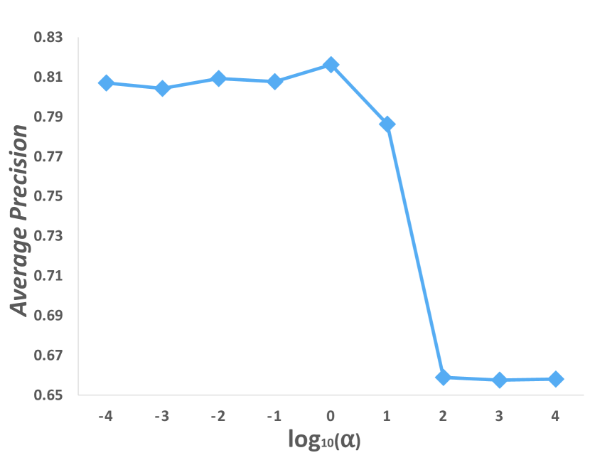
(a)  Average Precision

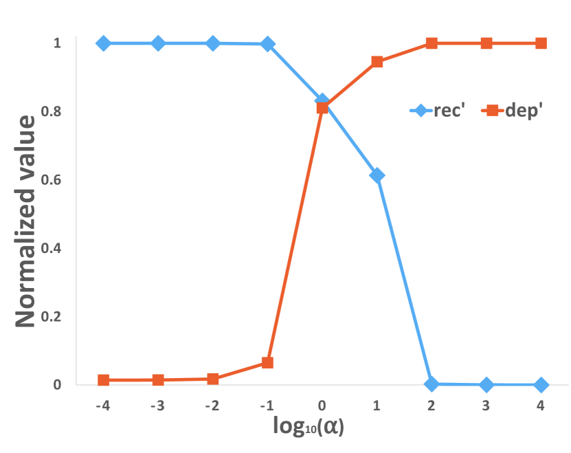
(b)  $dep^{\prime}$ and $rec^{\prime}$

Figure 1: Average precision changes as parameter $\alpha$ varies on msra.

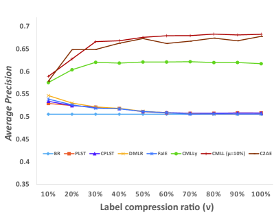
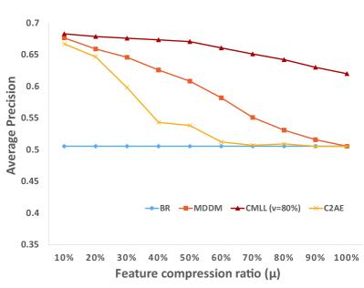
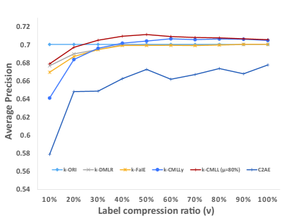
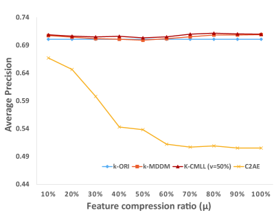
Figure 2: The average precision curve of moving the compression ratio on enron.

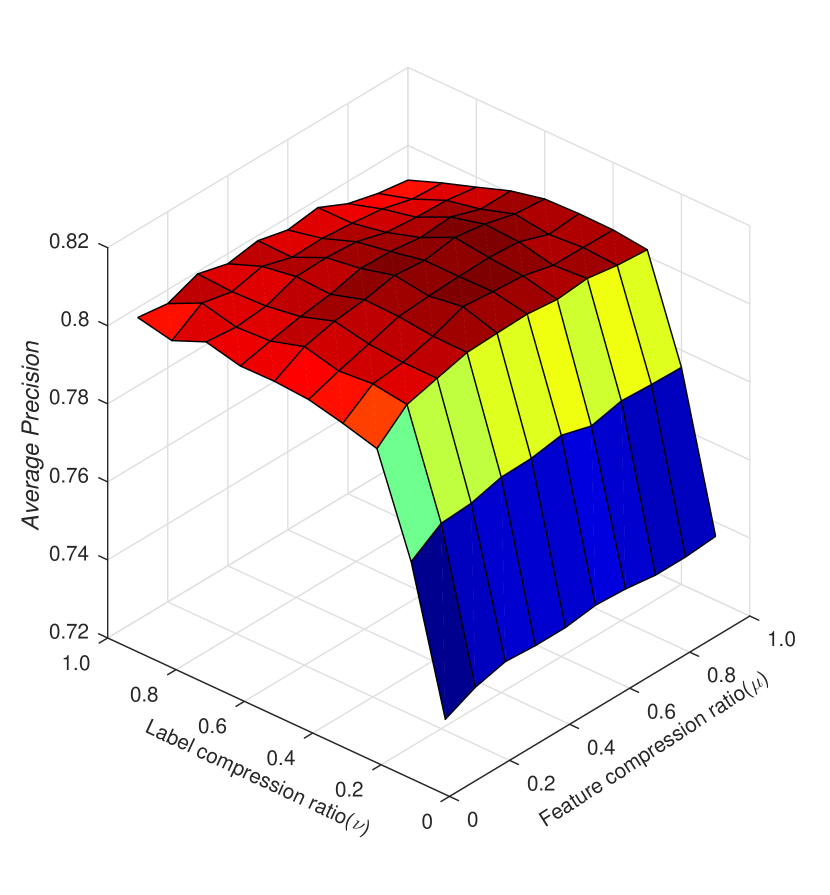
(a) msra

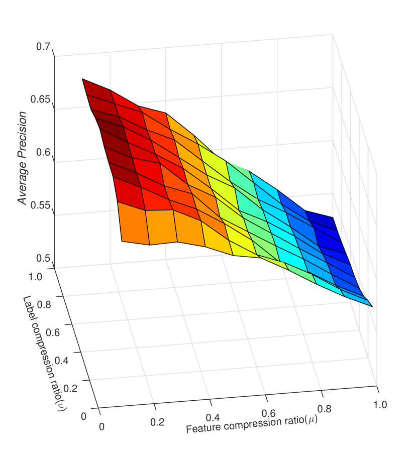
(b) enron

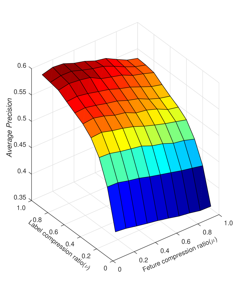
(c) bibtex

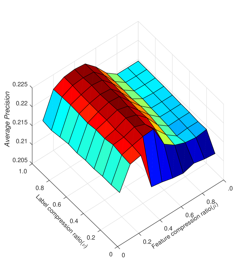
(d) esmpgame

Figure 3: The spatial graphs of CMLL over various $\mu$ and $\nu$.

5.3 Results

The experimental results of CMLL and k-CMLL compared with the comparing methods are shown in Table 2 and Table 3 respectively. For each metric, “$\downarrow$” indicates the smaller the better while “$\uparrow$” indicates the larger the better. We perform five-fold cross-validation on each dataset, and use paired $t$-test at 10% significance level. The mean results with standard deviation are reported and the best performance is highlighted in boldface. $\bullet/\circ$ represents whether CMLL or k-CMLL is significantly better/worse than the comparing methods. We can observe that across all metrics, CMLL ranks 1st in the most cases in both linear and non-linear cases.

As Table 2 and Table 3 show, with a suitable compression ratio, most embedding methods can achieve better performance than the baseline ORI. This indicates that there are indeed some problems such as sparsity and noise existing in both the original spaces, which leads to performance decline if not tackled properly. With a more compact representation for labels ($\nu\leq 100\%$) and features ($\mu\leq 100\%$), CMLL performs better than all compared LC methods ($\mu=100\%$) and FE method ($\nu=100\%$) in most cases. By applying the kernel trick to extend methods to their corresponding non-linear version, each LC method actually guides the embedding process of labels with the well transformed rather than the original features implicitly, where k-CMLL still outperforms other methods on the whole.

5.4 Parameter Sensitivity Analysis

To explore the influence of balance parameter $\alpha$ in CMLL, we fix $\mu=\nu=50\%$, $\lambda=0$ and run CMLL with $\alpha$ ranging in $\{10^{-4},10^{-3},...,10^{3},10^{4}\}$. To be convenient, we denote $dep=tr[\bm{V}^{t}\bm{HXP{P}^{t}{X}^{t}H}\bm{H}\bm{V}]$ and $rec=tr[\bm{V}^{t}\bm{YY}^{t}\bm{V}]$ as the dependence term and recovery term in objective (LABEL:eq:dual). Dropping the recovery term in (LABEL:eq:dual), we can find the solutions of $\bm{V}$ and $\bm{P}$, and then compute corresponding values of dependence term $dep_{max}$ and recovery term $rec_{min}$. Similarly, by only considering recover term in (LABEL:eq:dual), we can find the solution of $\bm{V}$ and calculate corresponding $dep_{min}$ and $rec_{max}$. To obtain a comprehensive understanding, we normalize the value of two terms by:

$$rec^{\prime}=\frac{rec-rec_{min}}{rec_{max}-rec_{min}},~{}~{}dep^{\prime}=\frac{dep-dep_{min}}{dep_{max}-dep_{min}}.$$

The experimental results on msra with average precision are showed in Fig. 1 as an example. The curve in Fig. 1 (a) indicates that setting $\alpha$ too big or too small will both result in bad performance. And it seems that an unreasonable big $\alpha$ suffers more, which indicates that an encoder with good recovery ability is very important for CMLL. Fig. 1 (b) provides the explanation for the curve trend in Fig. 1 (a). For example, the curve of average precision drops sharply when $log_{10}(\alpha)$ changes from 1 to 2. And the reason is that $dep^{\prime}$ is already very close to the upper bound when $\alpha=10$. As $\alpha$ further rises to $100$, the increment of $dep^{\prime}$ is very limited while $rec^{\prime}$ decreases obviously. This suggests that $\alpha$ do not need to be increased when $dep^{\prime}$ is close to its maximization, otherwise the decrement of $rec^{\prime}$ will result in a decline of the performance. Thus we can utilize such plot to guide the tuning process of $\alpha$. To sum up, aiming to get better performance, we should consider an appropriate trade-off between dependence term and recovery term.

5.5 Analysis on the Compression Ratio

We investigate how the compression ratio influence the performance, we fix one space changeless and gradually move the compression ration of the other space from 100% to 10%, and due to page limitation, we only display the curve of average precision on enron in Fig. 2. It can be seen that CMLL usually achieves a better or comparable performance, and other curves show similar results. The performance curves of metrics also reveal the effectiveness of the proposed method.

The reason for the superiority of CMLL is that it follows the spirit of CL. CMLL links the embedding process of the label space and the feature space to each other and guides each process by another well-disposed space. Instead, most other embedding methods either focus on the embedding of just one space, or guides the embedding process by original problematic space. Therefore, CMLL performs well especially in noisy, redundant and sparse datasets. However, the embedding may bring the loss of information when we compress the dense or non-redundant datasets into a very low dimension.

In reality, traversing every possible pair $(\mu,\nu)$ to lock the best one is unaffordable. Here we give an empirical method for that. We draw the spatial graphs of CMLL for collected datasets over various $\mu$ and $\nu$. And the spatial graphs of some datasets on average precision are displayed in Fig. 3 as examples.

It can be seen that, for different $\nu$ on each dataset, the general trends of CMLL over various $\mu$ are almost the same. Knowing this, we can first conduct CMLL with a fixed $\nu$ over various $\mu$, and lock the best $\mu^{*}$ in such situation. Then we can run CMLL with $\mu^{*}$ over various $\nu$ to find the best $\nu^{*}$. Finally near best ratio pair is given as $(\mu^{*},\nu^{*})$. One can also try some different starting $\nu$ to make the searching process more precise. In practice, we find that the ratio pair searched by this empirical method can achieve comparable performance to the real best one in most cases. Especially, we find that $\mu$ may have little influence on the performance in some datasets. In other words, a very small compression ratio can perform as well as other ratios in CMLL, which proves the existence of redundancy and shows the superiority of CMLL to reduce the computational and space complexities.

6 Conclusion

In this paper, we provided a different insight into the MLC for fully capturing the high-order correlation between features and labels, named compact learning. We analyzed its rationality and necessity in the situation, where the feature space suffers from redundancy or noise, and meanwhile, the label space is deteriorated by noise or sparsity - frequent occurrences in MLC. Following the spirit of compact learning, a simple yet effective method termed CMLL that is compatible with flexible multi-label classifiers was proposed. By conducting the embedding process of the features and the labels seamlessly, CMLL achieved a more compact representation for both the spaces. We demonstrated through experiments that CMLL can result in significant improvements for the multi-label classification.

As an initial effort towards compact learning, there are several potential ways that the current CMLL can be further improved: (a) Except the linear embedding or its kernel version, other encoding and decoding strategies, such as autoencoders and its extension, are worthwhile to be investigated; (b) Inspired by the manifold learning that the local topological structure can be shared between the feature manifold and the label manifold [34], the structure information could be utilized for CMLL; (c) CMLL provides another possible solution to some weakly supervised learning problem, e.g., the missing label [35] or noisy label [36].

References

- [1] M. Zhang, Z. Zhou, A review on multi-label learning algorithms, IEEE Transactions on Knowledge & Data Engineering 26 (8) (2014) 1819–1837.
- [2] F. Liu, T. Xiang, T. M. Hospedales, W. Yang, C. Sun, Semantic regularisation for recurrent image annotation, in: Proceedings of the 30th IEEE Conference on Computer Vision and Pattern Recognition, Honolulu, Hi, 2017, pp. 2872–2880.
- [3] Y. Liu, K. Wen, Q. Gao, X. Gao, F. Nie, Svm based multi-label learning with missing labels for image annotation, Pattern Recognition 78 (2018) 307–317.
- [4] K. Zhao, W. Chu, F. D. la Torre, J. F. Cohn, H. Zhang, Joint patch and multi-label learning for facial action unit and holistic expression recognition, IEEE Transactions on Image Processing 25 (8) (2016) 3931–3946.
- [5] N. Zhuang, Y. Yan, S. Chen, H. Wang, C. Shen, Multi-label learning based deep transfer neural network for facial attribute classification, Pattern Recognition 80 (2018) 225–240.
- [6] J. Liu, W. Chang, Y. Wu, Y. Yang, Deep learning for extreme multi-label text classification, in: Proceedings of the 40th International ACM SIGIR Conference on Research and Development in Information Retrieval, 2017, pp. 115–124.
- [7] X. Zhang, R. Henao, Z. Gan, Y. Li, L. Carin, Multi-label learning from medical plain text with convolutional residual models, arXiv preprint arXiv:1801.05062.
- [8] F. Tai, H. Lin, Multi-label classification with principal label space transformation, Neurocomputing 24 (9) (2012) 2508–2542.
- [9] B. Wang, L. Chen, W. Sun, K. Qin, K. Li, H. Zhou, Ranking-based autoencoder for extreme multi-label classification, arXiv preprint arXiv:1904.05937.
- [10] D. Hsu, S. Kakade, J. Langford, T. Zhang, Multi-label prediction via compressed sensing, in: Advances in Neural Information Processing Systems 22, Vancouver, Canada, 2009, pp. 772–780.
- [11] P. Rai, C. Hu, R. Henao, L. Carin, Large-scale bayesian multi-label learning via topic-based label embeddings, in: Advances in Neural Information Processing Systems 28, Montreal, Canada, 2015, pp. 3222–3230.
- [12] C. Yeh, W. Wu, W. Ko, Y. F. Wang, Learning deep latent space for multi-label classification, in: Proceedings of the 31st AAAI Conference on Artificial Intelligence, San Francisco, CA, 2017, pp. 2838–2844.
- [13] V. Kumar, A. K. Pujari, V. Padmanabhan, V. R. Kagita, Group preserving label embedding for multi-label classification, Pattern Recognition 90 (2019) 23–34.
- [14] J. Wicker, B. Pfahringer, S. Kramer, Multi-label classification using boolean matrix decomposition, in: ACM Symposium on Applied Computing, Trento, Italy, 2012, pp. 179–186.
- [15] X. Li, Y. Guo, Multi-label classification with feature-aware non-linear label space transformation, in: Proceedings of the 24th International Joint Conference on Artificial Intelligence, Buenos Aires, Argentina, 2015, pp. 3635–3642.
- [16] Y. Chen, H. Lin, Feature-aware label space dimension reduction for multi-label classification, in: Advances in Neural Information Processing Systems 25, Lake Tahoe, NV, 2012, pp. 1529–1537.
- [17] Z. Lin, G. Ding, M. Hu, J. Wang, Multi-label classification via feature-aware implicit label space encoding, in: Proceedings of the 31th International Conference on Machine Learning, Beijing, China, 2014, pp. 325–333.
- [18] D. R. Hardoon, S. Szedmak, J. Shawe-Taylor, Canonical correlation analysis: an overview with application to learning methods, Neurocomputing 16 (12) (2003) 2639–2664.
- [19] Y. Zhang, Z. Zhou, Multi-label dimensionality reduction via dependence maximization, ACM Transactions on Knowledge Discovery from Data 4 (3) (2010) 14.
- [20] L. Sun, S. Ji, J. Ye, Canonical correlation analysis for multilabel classification: A least-squares formulation, extensions, and analysis, IEEE Transactions on Pattern Analysis and Machine Intelligence 33 (1) (2010) 194–200.
- [21] Y. Zhang, J. Schneider, Multi-label output codes using canonical correlation analysis, in: Proceedings of the 14th International Conference on Artificial Intelligence and Statistics, Fort Lauderdale, FL, 2011, pp. 873–882.
- [22] J. Zhang, M. Fang, H. Wang, X. Li, Dependence maximization based label space dimension reduction for multi-label classification, Engineering Applications of Artificial Intelligence 45 (2015) 453–463.
- [23] A. Joly, P. Geurts, L. Wehenkel, Random forests with random projections of the output space for high dimensional multi-label classification, in: European Conference on Machine Learning and Principles and Practice of Knowledge Discovery in Databases, Nancy, France, 2014, pp. 607–622.
- [24] P. Mineiro, N. Karampatziakis, Fast label embeddings via randomized linear algebra, in: European Conference on Machine Learning and Principles and Practice of Knowledge Discovery in Databases, Porto, Portugal, 2015, pp. 37–51.
- [25] L. Jing, L. Yang, J. Yu, M. K. Ng, Semi-supervised low-rank mapping learning for multi-label classification, in: Proceedings of the 28th IEEE Conference on Computer Vision and Pattern Recognition, Boston, MA, 2015, pp. 1483–1491.
- [26] K. Bhatia, H. Jain, P. Kar, M. Varma, P. Jain, Sparse local embeddings for extreme multi-label classification, in: Advances in neural information processing systems 28, Montreal, Canada, 2015, pp. 730–738.
- [27] L. Jian, J. Li, K. Shu, H. Liu, Multi-label informed feature selection, in: Proceedings of the 25th International Joint Conference on Artificial Intelligence, New York, NY, 2016, pp. 1627–1633.
- [28] J. Wicker, A. Tyukin, S. Kramer, A nonlinear label compression and transformation method for multi-label classification using autoencoders, in: Pacific-Asia Conference on Knowledge Discovery and Data Mining, Auckland, New Zealand, 2016, pp. 328–340.
- [29] X. Shen, W. Liu, I. W. Tsang, Q. Sun, Y. Ong, Compact multi-label learning, in: Proceedings of 32nd AAAI Conference on Artificial Intelligence, New Orleans, LA, 2018, pp. 4066–4073.
- [30] A. Gretton, O. Bousquet, A. Smola, B. Schölkopf, Measuring statistical dependence with hilbert-schmidt norms, in: Proceedings of the 16th International Conference on Algorithmic Learning Theory, Singapore, 2005, pp. 63–77.
- [31] T. Hastie, R. Tibshirani, J. Friedman, The Elements of statistical learning: data mining, inference, and prediction, 2nd edition, Springer, 2004.
- [32] R. B. Lehoucq, D. C. Sorensen, Deflation techniques for an implicitly restarted arnoldi iteration, SIAM Journal on Matrix Analysis and Applications 17 (4) (1996) 789–821. doi:10.1137/S0895479895281484.
- [33] T. Wei, Y. Li, Learning compact model for large-scale multi-label data, in: Proceedings of the 33rd AAAI Conference on Artificial Intelligence, Vol. 33, Honolulu, HI, 2019, pp. 5385–5392.
- [34] P. Hou, X. Geng, M. Zhang, Multi-label manifold learning, in: Proceedings of the 30th AAAI Conference on Artificial Intelligence, Phoenix, Arizona, 2016, pp. 1680–1686.
- [35] J. Lv, N. Xu, R. Zheng, X. Geng, Weakly supervised multi-label learning via label enhancement., in: Proceedings of the 28th International Joint Conference on Artificial Intelligence, Macao, China, 2019, pp. 3101–3107.
- [36] G. Patrini, A. Rozza, A. K. Menon, R. Nock, L. Qu, Making deep neural networks robust to label noise: A loss correction approach, in: Proceedings of the 30th IEEE Conference on Computer Vision and Pattern Recognition, Honolulu, HI, 2017, pp. 1944–1952.