Multi-orbital-phase and multi-band characterization of exoplanetary atmospheres with reflected light spectra

Abstract

Direct imaging of widely separated exoplanets from space will obtain their reflected light spectra and measure atmospheric properties. Previous calculations have shown that a change in the orbital phase would cause a spectral signal, but whether this signal may be used to characterize the atmosphere has not been shown. We simulate starshade-enabled observations of the planet 47 UMa b, using the to-date most realistic simulator SISTER to estimate the uncertainties due to residual starlight, solar glint, and exozodiacal light. We then use the Bayesian retrieval algorithm ExoReL^ℜ to determine the constraints on the atmospheric properties from observations using a - or HabEx-like telescope, comparing the strategies to observe at multiple orbital phases or in multiple wavelength bands. With a $\sim 20\%$ bandwidth in 600 – 800 nm on a -like telescope, the retrieval finds a degenerate scenario with a lower gas abundance and a deeper or absent cloud than the truth. Repeating the observation at a different orbital phase or at a second 20% wavelength band in 800 – 1000 nm, with the same integration time and thus degraded S/N, would effectively eliminate this degenerate solution. Single observation with a HabEx-like telescope would yield high-precision constraints on the gas abundances and cloud properties, without the degenerate scenario. These results are also generally applicable to high-contrast spectroscopy with a coronagraph with a similar wavelength coverage and S/N, and can help design the wavelength bandwidth and the observation plan of exoplanet direct imaging experiments in the future.

1 Introduction

Direct imaging of exoplanets has begun to pick up momentum as a way to characterize exoplanetary atmospheres. High-contrast observations from the ground have measured thermal emission spectra of several exoplanets (Janson et al., 2010; Konopacky et al., 2013; Macintosh et al., 2015; Wagner et al., 2016; Rajan et al., 2017; Samland et al., 2017), and the spectra have shown the presence of carbon monoxide and water in their atmospheres. These planets are young giant planets so that they emit detectable thermal emission despite being well separated from their host stars.

Spaceborne direct-imaging capabilities in the future will enable atmospheric characterization in the reflected light. The , Spergel et al. (2015); Akeson et al. (2019)) will be capable of collecting starlight reflected by giant exoplanets through high-contrast imaging. The Starshade Rendezvous with (Seager et al., 2019), an advanced mission concept, would further enable to reach a planet-star contrast ratio as low as $\sim$10^-10. The (HabEx, Gaudi et al. (2020)), a concept of a 4-m space telescope with a starshade, has the main objective to image and study their atmospheres. Starshade Rendezvous and HabEx, both with a starshade, would allow studying giant exoplanets orbiting their host stars at about 1 – 10 AU with reflected light spectroscopy.

Reflected light spectra from these cold gaseous planets contain rich information on the chemical composition and cloud formation in their atmospheres (e.g., Sudarsky et al., 2000, 2003; Burrows et al., 2004; Cahoy et al., 2010; Lupu et al., 2016; MacDonald et al., 2018; Hu, 2019; Damiano & Hu, 2020; Carrión-González et al., 2020). When the wavelength coverage is limited and with moderate wavelength resolution and signal-to-noise ratio (S/N), there can be substantial degeneracy between the atmospheric abundance and the cloud pressure (e.g., Lupu et al., 2016; Nayak et al., 2017; Hu, 2019; Carrión-González et al., 2020). In short, a deep cloud and a small abundance of an absorber (e.g., CH₄) may result in a similar spectrum as a shallower cloud and a higher abundance of absorber, leading to the degeneracy.

A potential strategy to break the degeneracy is to observe the planets at multiple orbital phase angles. This is because viewing the same atmosphere at different phase angles would produce a wavelength-dependent difference in the spectra as the illumination and emerging angles have chromatic effects in atmospheric absorption and cloud reflection (Cahoy et al., 2010; Madhusudhan & Burrows, 2012; Nayak et al., 2017).

The reflected light spectra of Jupiter measured by telescopes from the center of the planet to the limb has led to constraints of the position and the vertical extent of the planet’s upper cloud layer (e.g., Sato & Hansen, 1979). Whether a similar measurement is as informative for exoplanets – disk integrated but viewed at different phase angles – is not well understood.

Here, we evaluate the multi-orbital-phase observations as a strategy to refine the constraints on the atmospheric properties from reflected light spectroscopy, and compare it to multi-wavelength-band observations Recognizing realistic operational overheads (e.g., the starshade would need to re-position itself precisely between the telescope and the star and this maneuver costs fuel), we specifically determine which of the following would produce the optimal science return when repeated observations are possible for an object of interest: We use the Starshade Imaging Simulation Toolkit for Exoplanet Reconnaissance (SISTER) to simulate data and uncertainties obtained in starshade-enabled spectroscopic observations. We then use a robust Bayesian inverse retrieval method (ExoReL^ℜ, Damiano & Hu, 2020) to determine and compare the information rendered by the three strategies.

The paper is organized as follows: Sec. 2 describes the simulation of the observed spectra and the multi-phase spectral retrieval method, Sec. 3 shows the results and compares the posterior constraints among the observation scenarios, and Sec. 4 discusses the observational strategy and summarizes the key findings of this study.

2 Methods

2.1 Simulated Planet Spectra

We use 47 UMa b, a giant planet orbiting a G0V star at 2.1 AU, as the representative planet in this study. 47 UMa b is in the design reference mission of both Starshade Rendezvous (Seager et al., 2019) and HabEx (Gaudi et al., 2020). Compared to Jupiter, 47 UMa b orbits closer to its host star and has a higher equilibrium temperature. In terms of cloud structure, this means that the upper atmosphere of the planet is expected to contain water clouds, as opposed to the ammonia clouds typical of Jupiter (Sudarsky et al., 2000). We simulated the atmospheric abundance and cloud structure of this exoplanet in our previous work (Damiano & Hu, 2020). Here we use ExoReL (Hu, 2019; Damiano & Hu, 2020) to synthesize the reflected light spectra at the orbital phases of $\pi/3$ and $\pi/2$. These phases are picked because the phase of $\pi/3$ is a good compromise between the angular separation between the planet and the star and the brightness in the reflected light (and thus the go-to phase of a single observation). The phase of $\pi/2$ is when the angular separation between the star and the planet is maximized. Should the planet be a Lambertian sphere, the brightness at $\pi/2$ is $\sim$50% of that at $\pi/3$; but our model calculates the wavelength-dependent phase function produced by clouds and gases in the atmosphere.

2.2 Simulated Uncertainties

A novel aspect of this study is the inclusion of realistic uncertainties expected from observations using a starshade. We use SISTER (Hildebrandt et al., in prep) to simulate the photons’ trajectory in the starshade-telescope system as well as detector effects in the telescope. Exposure time calculators (e.g., Robinson et al., 2016) have been developed to estimate the uncertainties of a starshade or coronagraph observation. However, they did not take into account the full 2-dimensional nature of the astrophysical scene nor the spatial variation of the Point Spread Function (PSF) due to the optical diffraction from the starshade. SISTER contemplates these aspects. Most details of SISTER can be found in its handbook. Our simulated astrophysical scene includes 47 UMa b, residual starlight, exozodiacal light (five times dustier than the Solar System, Ertel et al. (2020)), solar glint (i.e., scattered and reflected light from the Sun by the starshade, Hilgemann et al. (2019)), and local zodiacal light. Specifically, we consider petals of the starshade to have imperfection compatible with current lab work, which results in a greater residual starlight than an ideal starshade. We then place the planet as close as possible to the maximum intensity of the solar glint compatible with its orbital parameters. As such, we generate a scenario that serves as an upper limit for the integration time compared to other more favorable scenarios of the same system. Figure 1 shows the (noiseless) contribution of each component arriving at the detector.

On the telescope side, the optical throughput and the quantum efficiency (QE) of the detector follow the expected performance of and HabEx, respectively. The detector models an Electron Multiplying Charge Couple Device (EMCCD). The EMCCD gain factor is set to 1,000, making the read out noise effectively zero. We choose noise parameters corresponding to those adopted by and HabEx, respectively, including clock induced charge and dark current (Nemati et al., 2017).

When computing the uncertainties in the planetary counts, we assume that residual starlight, solar glint, exozodiacal light, and local zodiacal light can be subtracted out with some post-processing technique to the shot-noise limit, i.e., leaving no systematic bias in the measurements. This assumption increases the shot noise of these components by $\sim\sqrt{2}$ as a consequence of subtracting a noisy template from noisy data. The final error bars for each spectral bin are then derived from 1,000 independent SISTER simulations and used to generate independent Gaussian noise realizations, which are finally added to the input spectral data points.

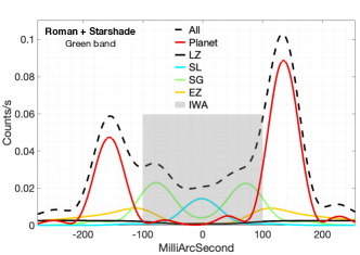
Figure 1: Contribution of each astrophysical and background component to the Starshade Rendezvous simulation performed by SISTER. The unit on the vertical axis is the rate of photons arriving at the instrument’s detector taking into account all the optical and instrumental effects, except noise, and has been integrated over the bandwidth. All is the sum of all individual contributions. Planet refers to the rate coming from the planet only. We plot on the left-hand side the planet when its orbital phase is $\pi/2$, and on the right-hand side when it is $\pi/3$. LZ refers to the contribution from the local zodiacal light at 22.5 V-mag/arcsec². SL is the contribution of the residual starlight from starshade imperfections. SG refers to the contribution from the solar glint for a representative angle of the Sun with respect to the target star. EZ is the contribution from the exozodiacal emission, which was chosen to be 5 times the of the Solar System. Finally, IWA refers to the geometric Inner Working Angle and is the apparent size of the starshade as seen by the telescope. Diffraction effects are relevant close and inside the IWA. Top: 0.61–0.75 $\mu$m. The planet-star flux ratio averaged over the bandwidth is 1.9$\times 10^{-8}$ when the orbital phase is $\pi/3$ and 1.0$\times 10^{-8}$ when it is $\pi/2$. The IWA is 100.2 mas. Bottom: 0.82–1.0 $\mu$m. The average planet-star flux ratio is 7.6$\times 10^{-9}$ when the orbital phase is $\pi/3$ and 4.2$\times 10^{-9}$ when it is $\pi/2$. The IWA is 130.4 mas. Notice that the photon rate is lower than in the 0.61–0.75 $\mu$m band.

We now turn to the specific scenarios that correspond to and HabEx.

2.2.1 Starshade Rendezvous with Roman

We consider a -like telescope with an Integral Field Spectrograph (IFS) that operates in 3 separate wavelength bands in 0.4 – 1.0 $\mu$m with a 20% bandwidth. We specifically assume “blue” (0.45–0.55 $\mu$m), “green” (0.61–0.75 $\mu$m), and “red” (0.82–1.0 $\mu$m) bands, all with resolving power $R=50$. These bands do not match exactly with the Coronagraph’s baseline design (V. Bailey, private comm.) or the design reference mission of the Starshade Rendezvous concept (Seager et al., 2019), as these designs have been evolving. In general, however, the blue band would cover the expected brightest section of the albedo spectrum and so is the best for planet detection, the green band would cover a strong absorption band of CH₄ and so is the primary band for atmospheric characterization, and the red band would provide additional information on CH₄ and cover an absorption band of H₂O (e.g., Lupu et al., 2016; MacDonald et al., 2018). With a 20% bandwidth, multiple observations would be necessary to obtain a spectrum that spans more than one band.

We determine the integration time by requiring an average S/N of 20 per spectral bin of the blue band when the orbital phase is $\pi/3$. The integration time is $\sim 3.5$ hours. We use this integration time in the other two bands, and in the observations with an orbital phase of $\pi/2$. We obtain an average S/N of 18.0 per spectral bin in the green band and 2.3 in the red band when the orbital phase is $\pi/3$. The S/N decreases to 11.5 and 1.5 when the orbital phase is $\pi/2$ (see Figure 3). The ratio of S/N between the 60-degree observation and the 90-degree observation is $\sim 1.55$ while the ratio of planetary flux is $\sim 2$. This is because the planetary flux contributes substantially to the shot noise in these observations, and the background fluxes from solar glint and exozodiacal dust decrease for wider angular separations from $\pi/3$ to $\pi/2$ (Figure 1).

2.2.2 HabEx

The HabEx concept (Gaudi et al., 2020) entails a larger telescope than that would be able to obtain spectra in a broad wavelength range between $0.45-1.0$ $\mu$m with a resolving power of $R=140$ with a single observation. The broader bandwidth and higher spectral resolution may provide improved constraints on atmospheric properties. The HabEx concept also entails a larger starshade than Rendezvous, and it would be placed further away from the telescope. This results in a decrease of the solar glint background, and this effect is included in SISTER. Here we evaluate whether multi-phase observations would further improve the constraints from single observation. The HabEx design includes an additional wavelength band at $1.0-1.8$ $\mu$m; we do not include this band in the analysis because it is primarily for characterizing small planets (Gaudi et al., 2020).

We simulate the uncertainties in HabEx simulations in a similar way as with . To compare the two cases, we adjust the integration time to obtain an average S/N of 20 per spectral bin in the 0.45–0.55 $\mu$m interval when the orbital phase is $\pi/3$. The integration time is $\sim 1.8$ hours. As in the case of , we use this integration time when the orbital phase is $\pi/2$. The average S/N per spectral bin in the 0.45–0.55 $\mu$m interval is 15.0 when the orbital phase is $\pi/2$ (see Figure 4).

2.3 Multi-Phase and Multi-Band Retrieval

We augment the ExoReL^ℜ retrieval framework (Damiano & Hu, 2020) with the ability to retrieve multiple spectra taken at different phase angles or in different wavelength bands. To simultaneously fit the spectra within the same Bayesian instance, we calculate the likelihood of each set of data and take the product. Specifically, when a set of free parameters is chosen to be evaluated, we calculate the spectrum for the first phase angle and we compare the model with the data to obtain the likelihood $\mathcal{L}_{1}$. With the same set of parameters we calculate the model referred to the second phase angle and we compare it to the data to calculate the likelihood $\mathcal{L}_{2}$. The product, $\mathcal{L}_{1}\times\mathcal{L}_{2}$ will give the total likelihood of the free parameters set, as

$$log(\mathcal{L})=log(\mathcal{L}_{1}\times\mathcal{L}_{2})=log(\mathcal{L}_{1})+log(\mathcal{L}_{2}).$$ (1)

Another update is that we now retrieve from the planet-star contrast ratio, rather than the albedo in Damiano & Hu (2020), because the uncertainties simulated are expressed in the planet-star contrast ratio. This brings in the planetary radius as a major factor. We now include the surface gravity as an additional free parameter in the retrieval, and the planetary radius is derived from the planetary mass and the retrieved surface gravity.

3 Results

Table 1: Results of the retrievals for each of the observational scenarios of Starshade Rendezvous with Roman considered for 47 UMa b. $\alpha$ is the phase angle. The reported errorbars are relative to the 95% confidence interval.

Parameters	Truths	Starshade Rendezvous with Roman
		Green band	Green band	Green & red bands	Green band
		$\alpha=\pi/3$ only	$\alpha=\pi/3$ & $\pi/2$	$\alpha=\pi/3$	$\alpha=\pi/3$ twice
$Log(H_{2}O)$	$-1.50$	$-1.18^{+1.07}_{-10.20}$	$-0.90^{+0.79}_{-1.60}$	$-0.98^{+0.84}_{-1.36}$	$-0.98^{+0.87}_{-1.21}$
$Log(NH_{3})$	$-2.36$	$-7.46^{+6.18}_{-4.16}$	$-6.29^{+5.65}_{-5.15}$	$-4.50^{+3.55}_{-6.64}$	$-6.90^{+5.49}_{-4.72}$
$Log(CH_{4})$	$-1.80$	$-1.45^{+1.13}_{-2.61}$	$-1.36^{+0.93}_{-1.61}$	$-1.43^{+1.02}_{-1.67}$	$-1.52^{+1.17}_{-1.12}$
$Log(P_{H_{2}O}[{\rm Pa}])$	$3.84$	$2.70^{+4.62}_{-2.43}$	$3.05^{+1.78}_{-2.13}$	$3.29^{+1.93}_{-2.15}$	$3.53^{+1.42}_{-2.85}$
$Log(D_{H_{2}O}[{\rm Pa}])$	$4.97$	$4.58^{+3.31}_{-3.66}$	$4.73^{+0.96}_{-0.49}$	$4.72^{+1.04}_{-0.49}$	$4.80^{+0.76}_{-0.64}$
$Log(CR_{H_{2}O})$	$-5.04$	$-7.93^{+6.59}_{-3.70}$	$-7.04^{+4.64}_{-4.33}$	$-7.36^{+4.98}_{-4.35}$	$-8.80^{+5.98}_{-2.96}$
$Log(g[{\rm cm/s^{2}}])$	$3.65$	$3.66^{+0.05}_{-0.04}$	$3.68^{+0.03}_{-0.03}$	$3.68^{+0.03}_{-0.04}$	$3.66^{+0.03}_{-0.06}$

Table 2: Results of the retrievals for each of the observational scenarios of HabEx considered for 47 UMa b. $\alpha$ is the phase angle. The reported errorbars are relative to the 95% confidence interval.

Parameters	Truths	HabEx
		$\alpha=\pi/3$	$\alpha=\pi/3$ &	$\alpha=\pi/3$
		only	$\alpha=\pi/2$	twice
$Log(H_{2}O)$	$-1.50$	$-1.60^{+0.58}_{-0.31}$	$-1.32^{+0.78}_{-0.40}$	$-1.30^{+0.71}_{-0.37}$
$Log(NH_{3})$	$-2.36$	$-2.78^{+0.98}_{-8.51}$	$-2.11^{+0.91}_{-6.43}$	$-2.51^{+0.82}_{-8.36}$
$Log(CH_{4})$	$-1.80$	$-1.76^{+0.36}_{-0.36}$	$-1.59^{+0.61}_{-0.33}$	$-1.62^{+0.51}_{-0.19}$
$Log(P_{H_{2}O}[{\rm Pa}])$	$3.84$	$2.52^{+1.50}_{-1.95}$	$2.22^{+1.48}_{-1.95}$	$2.44^{+1.34}_{-1.74}$
$Log(D_{H_{2}O}[{\rm Pa}])$	$4.97$	$5.00^{+0.24}_{-0.16}$	$4.96^{+0.16}_{-0.24}$	$4.96^{+0.07}_{-0.16}$
$Log(CR_{H_{2}O})$	$-5.04$	$-8.75^{+4.94}_{-3.04}$	$-9.21^{+4.77}_{-2.65}$	$-9.18^{+4.88}_{-2.69}$
$Log(g[{\rm cm/s^{2}}])$	$3.65$	$3.65^{+0.02}_{-0.01}$	$3.66^{+0.02}_{-0.01}$	$3.66^{+0.02}_{-0.01}$

The constraints on the atmospheric properties retrieved from the simulated observations with Starshade Rendezvous with and HabEx are summarized in Tables 1 and 2 and shown in Figures 3 and 4. Definitions of these parameters and their impact on the albedo spectrum are described in detail in Damiano & Hu (2020). Briefly, $Log(H_{2}O)$, $Log(NH_{3})$, and $Log(CH_{4})$ are the mixing ratios of the trace gases; since we include condensation of H₂O, the mixing ratio of H₂O is the mixing ratio below the cloud. $Log(P_{H_{2}O})$ and $Log(D_{H_{2}O})$ are the top pressure and depth of the H₂O cloud. The cloud depth is the difference in pressure between the bottom and the top of the cloud. $Log(CR_{H_{2}O})$ is the ratio between the mixing ratio of H₂O above the cloud and that below the cloud – the difference is condensed out to form the cloud.

. The most plausible starting point to characterize the atmosphere of 47 UMa b in reflected light is a single observation in the green band. Our retrieval analysis in this scenario finds a solution close to the truth, as well as a degenerate solution (dashed blue lines in Figure 2 and 3). While the truth has a mixing ratio of CH₄ of $\sim 10^{-2}$ and a H₂O cloud at $0.1\sim 1$ bar, the degenerate solution has a mixing ratio of CH₄ of $\sim 10^{-4}$ and corresponding mixing ratio of H₂O $<10^{-6}$ (Figure 3). With such a low abundance of water, there is not enough mass to form a reflective cloud, and so the degenerate solution is insensitive to the cloud description parameters ($Log(P_{H_{2}O})$, $Log(D_{H_{2}O})$, and $Log(CR_{H_{2}O})$). The degenerate solution is essentially a cloud-free atmosphere with the mixing ratio of CH₄ two-order-of-magnitude lower than the truth.

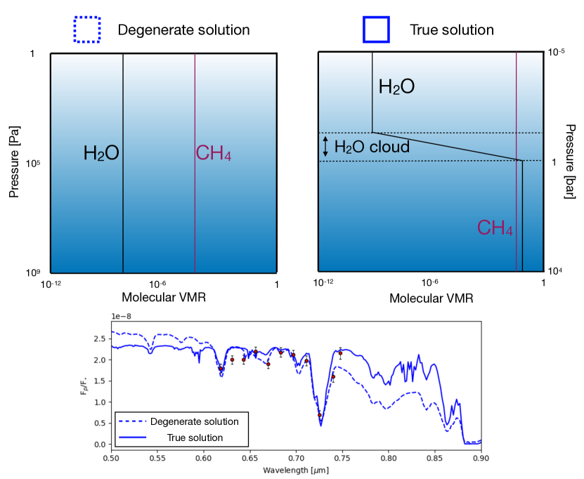
Figure 2:

Adding a second observation at a different orbital phase ($\alpha=\pi/2$ in this study) with the same integration time would drastically reduce the likelihood of the degenerate solution. The S/N of the second observation is poorer, because the baseline of the spectrum is lower at the phase of $\alpha=\pi/2$ than at the phase of $\alpha=\pi/3$. The simultaneous retrieval of the observations at both phases would find the true result (see the orange model and distributions shown in Figure 3). The improvement in the constraints comes from two factors. First, adding a second observation inevitably increase the S/N of the overall observation, which helps eliminate the degenerate solution. Second, the true and the degenerate scenarios have different achromatic phase functions, and the biggest difference occurs at the main absorption bands (Figure 3). The difference is on the order of 5%, so that the S/N of 11.5 per spectral bin from the assumed observational scenario could partly leverage this diagnostic power.

Moreover, adding an observation in the red band with the same integration time would also drastically reduce the significance of the degenerate solution almost to zero. Here we assume that the second observation takes place immediately after the first one, and they essentially correspond to the same orbital phase. The red-band observation has an average S/N of only $\sim 2$, due to decreasing starlight intensity, lower planetary albedo, stronger solar glint, and degrading detector quantum efficiency from the green band to the red band. Despite the poor S/N of the red-band spectrum, we find it highly informative when combined with the green-band spectrum. The retrieval of the observations at both bands does not show a degenerate solution (see the green model and distributions shown in Figure 3). This is because the degenerate scenario has a much lower albedo than the truth in the red band, and the difference is well on the order of 30% in 0.75 – 0.85 $\mu$m.

The last scenario considered is to repeat the first observation at the same wavelength band and at the same orbital phase, i.e., a second realization. The combined S/N is $\sim 25$ per spectral bin, and to our surprise, this strategy would also eliminate the degenerate solution. Most of the diagnosing power comes from the datum at 0.75 $\mu$m, where the truth and the degenerate scenario differ the most.

As long as the degenerate solution is eliminated, the reflected light spectral retrieval can constrain not only the mixing ratio of CH₄ in the atmosphere, but also the mixing ratio of H₂O below the cloud (as it is the feedstock for cloud), and the pressure level of the cloud. There is a moderate correlation between the mixing ratio of CH₄ and the pressure level of the cloud (Figure 3). Inferring the mixing ratio of H₂O below the cloud is possible because our retrieval method preserves the causal relationship between the condensation of water vapor and the formation of a water cloud (Damiano & Hu, 2020). The surface gravity, and thus the radius of the planet is constrained in all scenarios.

HabEx. A single observation of HabEx with a S/N of $\sim 20$ would pinpoint the atmospheric properties (see the blue model and distributions shown in Figure 4). Specifically, the mixing ratios of CH₄ and H₂O would be well constrained to the precision of $\sim 1/3$ dec, and that of the cloud pressure would be better constrained than $\sim 1/5$ dec. There is no correlation between the mixing ratio of CH₄ and the cloud pressure in this case. Notably, the spectrum yields meaningful constraints on the mixing ratio of NH₃, mostly from the small absorption feature at $\sim 0.63$ $\mu$m. These improvements come from not only the broader wavelength coverage and the higher spectral resolution than , but also the larger and further starshade (for lower solar glint) and the larger telescope aperture (for lower exozodiacal light). Adding another observation with at the same or a different orbital phase would slightly reduce uncertainty in the retrieved mixing ratios of CH₄, while the overall gain in the constraints of the parameters is minimal.

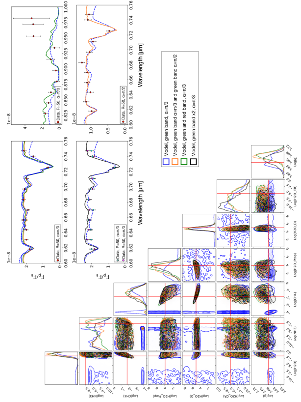
Figure 3: Retrieval analysis of the four observational scenarios of Starshade Rendezvous with . The four panels on the top show the best-fit models and the simulated data. The dashed blue line in the first panel shows the degenerate solution obtained with a single observation in the green band and at the orbital phase of $\pi/3$; the other three panels show how this solution may be inconsistent with additional observations. The corner plot on the bottom shows the marginalized posterior distribution for each of the parameters, using the same color scheme to denote the four observational scenarios simulated. The degenerate solution is eliminated with a second observation at the same phase, at a wider-separated phase of $\pi/2$, or in the red band.

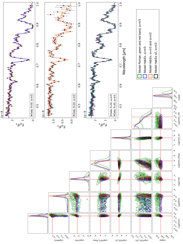
Figure 4: Retrieval analysis of the three observational scenarios of HabEx. The three panels on the top show the best-fit models and the simulated data. The corner plot on the bottom shows the marginalized posterior distribution for each of the parameters, using the same color scheme to denote the three observational scenarios simulated. The green model in the corner plot is the same as the green model in Figure 3, and it is shown for comparison. A single observation with HabEx would be sufficient to constrain the atmospheric properties.

4 Discussion & Conclusion

With the case studies presented in Section 3, we show that with a limited wavelength band like the green band on , a single observation of a planet’s reflected light spectrum at the favorable orbital phase (e.g., $\alpha=\pi/3$) and a high S/N (e.g., $\sim$20) can result in degenerate solutions. The degeneracy is between the atmospheric scenario of a higher cloud and greater mixing ratio of CH₄ versus the scenario of a lower or absent cloud and smaller mixing ratio of CH₄. This type of degeneracy has been discussed in Hu (2014, 2019) and it is shown here with realistic noise estimates and rigorous retrieval.

Expanding the wavelength coverage to longer wavelengths (i.e., the red band), doubling the integration time, or repeating the observation at a different orbital phase with a similar integration time would be able to eliminate this degeneracy. As shown in Section 3, these three strategies result in similar-quality constraints on the atmospheric parameters.

Particularly, the spectra that are degenerate in the green band diverge at longer wavelengths: the low or absent cloud scenario would have a much lower albedo than the high cloud scenario. The divergence is often so significant that even a low S/N observation at the long wavelengths can effectively eliminate the degenerate solution. To date, it is often assumed that the red-band observation with would be severely affected by the degrading quantum efficiency of the detector in this band (e.g., Seager et al., 2019). Here we show that even with the poor quantum efficiency and other complications, a red-band observation with the same integration time as the green band can be highly informative. This finding also implies that the constraints on the atmospheric properties would be drastically improved at no additional integration time, if the wavelength bandwidth could be enlarged to cover both the green band and the red band with a single observation.

If broadening the wavelength coverage is not possible, eliminating the degenerate solution would require an S/N per spectral bin of at least $\sim 25$, which may be achieved by integrating longer in a single observation or revisiting the same planet at a different orbital phase. At an S/N of $\sim 18$ per visit, the difference between revisiting and integrating longer is minimal, and thus integrating longer may be the preferred strategy to avoid re-targeting the starshade. As shown in Fig. 3, there is indeed a difference in the spectral features between the two phases, consistent with Cahoy et al. (2010). To capture this subtle difference, however, will require a high S/N ($>20$) on the observations at both orbital phases and thus a longer integration time for the observation at the less-than-optimal phase. The analysis here highlights that, when only one observation in a limited wavelength bandwidth is expected, it is important to schedule that observation at the phase that maximizes the S/N of the spectrum and with sufficient duration.

With a wide wavelength coverage in the visible and near-infrared, a HabEx-like telescope would provide precise constraints on the atmospheric gas abundances and cloud properties in widely separated giant exoplanets with one observation of the reflected light, without the degeneracy between the gas abundance and the cloud pressure as discussed above. Not knowing the planetary radius does not substantially affect this capability. To our knowledge, this is the first time such capability is demonstrated with realistic uncertainty estimates and Bayesian retrievals. Also, as we have shown in Damiano & Hu (2020), the abundance of the cloud-forming gas (e.g., H₂O in 47 UMa b) below the cloud can be constrained from the reflected light spectra.

In conclusion, we present simulations of starshade-enabled reflected light spectroscopy of widely separated giant exoplanets and use Bayesian retrievals to assess strategies to improve the constraints on the atmospheric properties. We show that a degenerate scenario with a lower gas abundance and a deeper or absent cloud than the truth can be retrieved when the observation is limited to a $\sim 20\%$ band in 600 – 800 nm and has an S/N of $\sim 18$. Widening the wavelength coverage to include 800 – 1000 nm is the most effective way to eliminate the degenerate solution. Doubling the integration time or repeating the observation at a different, less-than-optimal orbital phase would also eliminate the degenerate solution. Although these results are based on starshade simulations, they are generally applicable to high-contrast imaging and spectroscopy with a coronagraph with similar wavelength coverage, spectral resolution, and S/N. The work presented here will be important to design and define the wavelength bandwidth and the observation plan of exoplanet direct imaging experiments in the future.

References

- Akeson et al. (2019) Akeson, R., Armus, L., Bachelet, E., et al. 2019, arXiv e-prints, arXiv:1902.05569. https://arxiv.org/abs/1902.05569
- Burrows et al. (2004) Burrows, A., Sudarsky, D., & Hubeny, I. 2004, ApJ, 609, 407, doi: 10.1086/420974
- Cahoy et al. (2010) Cahoy, K. L., Marley, M. S., & Fortney, J. J. 2010, ApJ, 724, 189, doi: 10.1088/0004-637X/724/1/189
- Carrión-González et al. (2020) Carrión-González, Ó., Muñoz, A. G., Cabrera, J., et al. 2020, Astronomy & Astrophysics, 640, A136
- Damiano & Hu (2020) Damiano, M., & Hu, R. 2020, AJ, 159, 175, doi: 10.3847/1538-3881/ab79a5
- Ertel et al. (2020) Ertel, S., Defrère, D., Hinz, P., et al. 2020, AJ, 159, 177, doi: 10.3847/1538-3881/ab7817
- Gaudi et al. (2020) Gaudi, B. S., Seager, S., Mennesson, B., et al. 2020, arXiv e-prints, arXiv:2001.06683. https://arxiv.org/abs/2001.06683
- Hilgemann et al. (2019) Hilgemann, E., Shaklan, S., McKeithen, D., et al. 2019, NASA Starshade Technology Development Activity Milestone Report, 3, https://exoplanets.nasa.gov/internal_resources/1544/
- Hu (2014) Hu, R. 2014, arXiv e-prints, arXiv:1412.7582. https://arxiv.org/abs/1412.7582
- Hu (2019) —. 2019, ApJ, 887, 166, doi: 10.3847/1538-4357/ab58c7
- Janson et al. (2010) Janson, M., Bergfors, C., Goto, M., Brandner, W., & Lafrenière, D. 2010, ApJ, 710, L35, doi: 10.1088/2041-8205/710/1/L35
- Konopacky et al. (2013) Konopacky, Q. M., Barman, T. S., Macintosh, B. A., & Marois, C. 2013, Science, 339, 1398, doi: 10.1126/science.1232003
- Lupu et al. (2016) Lupu, R. E., Marley, M. S., Lewis, N., et al. 2016, AJ, 152, 217, doi: 10.3847/0004-6256/152/6/217
- MacDonald et al. (2018) MacDonald, R. J., Marley, M. S., Fortney, J. J., & Lewis, N. K. 2018, ApJ, 858, 69, doi: 10.3847/1538-4357/aabb05
- Macintosh et al. (2015) Macintosh, B., Graham, J. R., Barman, T., et al. 2015, Science, 350, 64, doi: 10.1126/science.aac5891
- Madhusudhan & Burrows (2012) Madhusudhan, N., & Burrows, A. 2012, ApJ, 747, 25, doi: 10.1088/0004-637X/747/1/25
- Nayak et al. (2017) Nayak, M., Lupu, R., Marley, M. S., et al. 2017, PASP, 129, 034401, doi: 10.1088/1538-3873/129/973/034401
- Nemati et al. (2017) Nemati, B., Krist, J. E., & Mennesson, B. 2017, in Society of Photo-Optical Instrumentation Engineers (SPIE) Conference Series, Vol. 10400, Proc. SPIE, 1040007
- Rajan et al. (2017) Rajan, A., Rameau, J., De Rosa, R. J., et al. 2017, AJ, 154, 10, doi: 10.3847/1538-3881/aa74db
- Robinson et al. (2016) Robinson, T. D., Stapelfeldt, K. R., & Marley, M. S. 2016, PASP, 128, 025003, doi: 10.1088/1538-3873/128/960/025003
- Samland et al. (2017) Samland, M., Mollière, P., Bonnefoy, M., et al. 2017, A&A, 603, A57, doi: 10.1051/0004-6361/201629767
- Sato & Hansen (1979) Sato, M., & Hansen, J. E. 1979, Journal of Atmospheric Sciences, 36, 1133, doi: 10.1175/1520-0469(1979)036<1133:JACACS>2.0.CO;2
- Seager et al. (2019) Seager, S., Kasdin, N. J., Booth, J., et al. 2019, in BAAS, Vol. 51, 106
- Spergel et al. (2015) Spergel, D., Gehrels, N., Baltay, C., et al. 2015, arXiv e-prints, arXiv:1503.03757. https://arxiv.org/abs/1503.03757
- Sudarsky et al. (2003) Sudarsky, D., Burrows, A., & Hubeny, I. 2003, ApJ, 588, 1121, doi: 10.1086/374331
- Sudarsky et al. (2000) Sudarsky, D., Burrows, A., & Pinto, P. 2000, ApJ, 538, 885, doi: 10.1086/309160
- Wagner et al. (2016) Wagner, K., Apai, D., Kasper, M., et al. 2016, Science, 353, 673, doi: 10.1126/science.aaf9671