SISTA: learning optimal transport costs under sparsity constraints

Abstract.

In this paper, we describe a novel iterative procedure called SISTA to learn the underlying cost in optimal transport problems. SISTA is a hybrid between two classical methods, coordinate descent (“S”-inkhorn) and proximal gradient descent (“ISTA”). It alternates between a phase of exact minimization over the transport potentials and a phase of proximal gradient descent over the parameters of the transport cost. We prove that this method converges linearly, and we illustrate on simulated examples that it is significantly faster than both coordinate descent and ISTA. We apply it to estimating a model of migration, which predicts the flow of migrants using country-specific characteristics and pairwise measures of dissimilarity between countries. This application demonstrates the effectiveness of machine learning in quantitative social sciences.

Keywords: inverse optimal transport, coordinate descent, ISTA

1. Introduction

Optimal transport has received a great deal of attention recently, see [22], [23], [21], and [11]. The discrete version of the problem in a nutshell is as follows. Consider a $N\times N$ matrix $c_{ij}$ called a transport cost, which is the cost of pairing $i\in\left\{1,...,N\right\}$ with $j\in\left\{1,...,N\right\}$, and consider two marginal probability distributions $p$ and $q$ with support $\left\{1,...,N\right\}$. The optimal transport problem is the problem of finding the optimal transport plan, the joint probability distribution $\pi_{ij}$ over $\left\{1,...,N\right\}^{2}$ which is optimal in the sense that $\sum_{1\leq i,j\leq N}\pi_{ij}c_{ij}$ is minimal over all the probability $\pi$ with marginal distributions $p$ and $q$. A variant of this problem where one seeks to minimize the cost with a regularizing entropy term, namely $\sum_{1\leq i,j\leq N}\pi_{ij}c_{ij}+T\pi_{ij}\ln\pi_{ij}$, with $T>0$ being a temperature parameter, has been proposed by various authors and has been found to enjoy attractive computational and statistical properties, see e.g. [16] and references therein.

Most of the literature on optimal transport takes the transport cost matrix $c$ as given and seeks to compute the optimal transport plan $\pi$. However, in some situations, one observes $\pi$ and would like to learn the cost $c$. This problem, which belongs to the general class of “inverse problems,” see [15], arises in particular in economics, see [12], where one observes optimally matched agents and one would like to infer why they have chosen to match. The problem of learning the transport cost has received relatively little attention in the machine learning literature. Some exceptions are [8], who use a Difference of Convex (DC) functions approach, [14], who use a strategy based on Neighborhood Components Analysis (NCA), and [10], who compute a rank-regularized moment matching estimator of the ground distance using proximal gradient descent.

In this paper, we assume that the transportation cost $c_{ij}$ takes a parametric form $c_{ij}^{\beta}$, where the parameter vector $\beta$ is assumed to be sparse. We introduce an iterative procedure to estimate $\beta$ by minimizing a convex loss function under an $l_{1}$ penalization based on the dual formulation of the optimal transport problem. Our procedure is a hybrid between coordinate descent and proximal gradient descent: indeed, a phase of exact minimization with respect to the transport potentials alternates with a phase of proximal gradient descent (ISTA, see [1]) with respect to the parameters of the transport cost. This procedure is thus a natural extension of the celebrated Sinkhorn algorithm (see an account in [19] and a historical overview in [16]), a.k.a. the Iterative Proportional Fitting Procedure (IPFP), which is a coordinate descent algorithm with respect to the transport potentials, for a fixed value of the parameter vector. One important advantage of the Sinkhorn algorithm compared with alternative methods is that it is fast, parameteter-free and can be naturally parallelized, as documented for example in [7] and [6].

The remainder of the paper is organized as follows. Section 2 presents the optimal transport problem, recalls duality results, and introduces the inverse problem of learning the parameter vector of the transport cost under an $l_{1}$ penalization. Section 3 describes the SISTA algorithm, states results on its linear convergence, and benchmarks its speed of convergence via numerical experiments. Section 4 applies this procedure to a model of migration based on country-specific characteristics and pairwise measures of dissimilarity between countries. Section 5 concludes the paper.

2. Optimal transport with entropic regularization

2.1. Problem formulation

Consider two discrete probability distributions $p$ and $q$ supported by $N$ points. The optimal transport problem between $p$ and $q$, see [22], is classically defined as

$$\min_{\pi\in\Pi}\sum_{1\leq i,j\leq N}\pi_{ij}c_{ij}$$ (1)

where $c_{ij}$ is the transport cost from $i$ to $j$, and $\Pi$ is the set of probability mass vectors $\pi$ with margins $p$ and $q$, that is

$$\Pi=\left\{\pi_{ij}\geq 0:\sum_{j=1}^{N}\pi_{ij}=p_{i}\text{ and }\sum_{i=1}^{N}\pi_{ij}=q_{j}\right\}.$$ (2)

Recently, the literature (see for instance [12] and [7]) has considered the entropic regularization of (1), that is

$$\min_{\pi\in\Pi}\sum_{1\leq i,j\leq N}\pi_{ij}c_{ij}+T\pi_{ij}\ln\pi_{ij}$$ (3)

where $T>0$ is a temperature parameter, so that $T\rightarrow 0$ recovers the previous object. The dual version of (3) is

$$\max_{u,v}\sum_{i=1}^{N}p_{i}u_{i}+\sum_{j=1}^{N}q_{j}v_{j}-T\sum_{1\leq i,j\leq N}\exp\left(\frac{u_{i}+v_{j}-c_{ij}}{T}\right).$$ (4)

Note that by homogeneity, the solution of problem (3) is left invariant by dividing $c$ and $T$ by the same constant. Taking this constant to be $T$, we can without loss of generality set

$$T=1,$$ (5)

which we will do in the sequel. After taking the negative, we obtain the following dual optimization problem

$$\min_{u,v}\sum_{1\leq i,j\leq N}\exp\left(u_{i}+v_{j}-c_{ij}\right)-\sum_{i=1}^{N}p_{i}u_{i}-\sum_{j=1}^{N}q_{j}v_{j}.$$ (6)

By first order conditions, the optimal $\pi$ in (3) and the optimal $\left(u,v\right)$ in (6) are such that

$$\pi_{ij}=\exp\left(u_{i}+v_{j}-c_{ij}\right),$$ (7)

where $u$ and $v$ are adjusted so that the primal constraints are satisfied, i.e. $\pi\in\Pi$ as in (2).

The dual problem (6) is a convex minimization problem, which can be solved by gradient descent. However, it is well-known that blockwise coordinate descent over $u$ and $v$ iteratively, a procedure called Sinkhorn’s algorithm, see [19] and references therein, is a preferable alternative. Given $\left(u^{t},v^{t}\right)$, the minimization of problem (6) with respect to $u_{i}$ yields, by first order conditions,

$$\exp\left(u_{i}^{t+1}\right)=\frac{p_{i}}{\sum_{j=1}^{N}\exp\left(v_{j}^{t}-c_{ij}\right)},$$ (8)

while the minimization of (6) with respect to $v_{j}$ yields

$$\exp\left(v_{j}^{t+1}\right)=\frac{q_{j}}{\sum_{i=1}^{N}\exp\left(u_{i}^{t+1}-c_{ij}\right)}.$$ (9)

Alternating the minimization steps with respect to $u_{i}$ and $v_{j}$ therefore yields to alternating between the closed-form updating formulas (8) and (9).

2.2. Learning the transport cost

We now turn to the inverse problem of recovering the transport cost $c_{ij}^{\beta}$ based on the observed transport plan $\hat{\pi}\in\Pi$. To achieve this, we assume that the cost function can be represented by a linear combination of basis functions $d^{k}$, $k\in\left\{1,...,K\right\}$ as

$$c_{ij}^{\beta}=\sum_{k=1}^{K}\beta_{k}d_{ij}^{k},$$ (10)

where each $d_{ij}^{k}$ is some measure of dissimilarity between $i$ and $j$, and $\beta=(\beta_{1},\cdots,\beta_{K})^{\top}$ is a parameter vector to be learned.

We present a few choices of dissimilarity measures $d_{ij}^{k}$.

(a). If $x^{i}$ and $y^{j}$ are vectors of characteristics for $i$ and $j$, one may set $d_{ij}^{k}=\left(x^{i}_{k}-y^{j}_{k}\right)^{2}$, where the subscript $k$ denotes the $k$-th component of a vector.

(b). Similarly, if $k=(r,s)$ stands for a pair of indices, one may set $d_{ij}^{rs}=\left(x_{r}^{i}-y_{s}^{j}\right)^{2}$ as is done in [9], in order to capture off-diagonal interactions between characteristics. The matrix parameter $\beta_{rs}$ to be learned measures the interaction between two distinct characteristics.

(c). If, like in our application, $i$ and $j$ are countries, then $d_{ij}^{k}$ may be the share of inhabitants of country $i$ who do not speak the language of country $j$. Note that this measure has no reason to be symmetric since $d_{ij}^{k}\neq d_{ji}^{k}$ in general.

Our learning procedure is based on looking for $\beta$ such that $\pi_{ij}^{\beta}=\exp\left(u_{i}+v_{j}-c_{ij}^{\beta}\right)$ solves the margin constraints $\pi^{\beta}\in\Pi$, and matches the moments of $d^{k}$ for $k=1,...,K$, that is

$$\sum_{i=1}^{N}\pi_{ij}^{\beta}=q_{j},\sum_{j=1}^{N}\pi_{ij}^{\beta}=p_{i},\sum_{1\leq i,j\leq N}\pi_{ij}^{\beta}d_{ij}^{k}=\sum_{1\leq i,j\leq N}\hat{\pi}_{ij}d_{ij}^{k}.$$ (11)

As shown by [12], equations (11) arise as the first order conditions of the following minimization problem

$$\min_{u,v,\beta}F\left(u,v,\beta\right),$$ (12)

where

$$F\left(u,v,\beta\right):=\sum_{1\leq i,j\leq N}\exp\left(u_{i}+v_{j}-c_{ij}^{\beta}\right)+\sum_{1\leq i,j\leq N}\hat{\pi}_{ij}\left(c_{ij}^{\beta}-u_{i}-v_{j}\right)$$ (13)

is a convex function.

Now assuming that $\beta$, the parameter vector, is sparse, one way to handle this problem is to add the $l_{1}$ penalty term in (12), namely considering the following problem:

$$\min_{u,v,\beta}\Phi\left(u,v,\beta\right):=F\left(u,v,\beta\right)+\gamma\left|\beta\right|_{1},$$ (14)

where $\gamma$ is a regularization parameter. This regularization is similar in spirit to [10], who have introduced a rank regularization technique using the nuclear norm in a problem where $\beta$ is a matrix. In the next section, we provide the SISTA algorithm for the computation of (14).

3. SISTA

3.1. Algorithm

The SISTA algorithm consists of the minimization of $\Phi\left(u,v,\beta\right)$ in (14) by iterating three alternating phases:

• an exact minimization of with respect to $u$, holding $\beta$ and $v$ constant;

• an exact minimization of with respect to $v$, holding $\beta$ and $u$ constant;

• a proximal gradient descent step with respect to $\beta$, holding $u$ and $v$ constant.

Each of these three phases is straightforward. The exact minimization with respect to $u$ is done in closed-form by the updating formula (8) and for $v$ done by (9). The proximal gradient descent step with respect to $\beta$ yields

$$\beta^{t+1}=\text{prox}_{\rho\gamma|\cdot|_{1}}\left(\beta^{t}-\rho\nabla_{\beta}F\left(u^{t+1},v^{t+1},\beta^{t}\right)\right),$$

which is explicit and whose components are given by the well-known soft-thresholding formula:

$$\text{prox}_{\rho\gamma|\cdot|}(z)=\begin{cases}z-\rho\gamma&\text{if }z>\rho\gamma\\ 0&\text{if }|z|\leq\rho\gamma\\ z+\rho\gamma&\text{if }z<-\rho\gamma\end{cases}.$$

Combining these three steps yields SISTA, which we describe in algorithm 1.

Algorithm 1 The SISTA algorithm

Initial guess of parameter vector $\beta^{0}$, of potentials $u^{0}$ and $v^{0}$, step size $\rho$, and dissimilarity measures $d_{ij}^{k}$

while not converged do

     (Sinkhorn step). Set $c^{\beta^{t}}_{ij}:=\sum_{k=1}^{K}\beta_{k}^{t}d_{ij}^{k}$ and update:

$$\left\{\begin{array}[]{l}\exp\left(u_{i}^{t+1}\right)=\frac{p_{i}}{\sum_{j=1}^{N}\exp\left(v_{j}^{t}-c_{ij}^{\beta^{t}}\right)}\\ \exp\left(v_{j}^{t+1}\right)=\frac{q_{j}}{\sum_{i=1}^{N}\exp\left(u_{i}^{t+1}-c_{ij}^{\beta^{t}}\right)}\end{array}\right.$$

     (ISTA step). Let $\pi_{ij}^{\beta^{t}}:=\exp\left(u_{i}^{t+1}+v_{j}^{t+1}-c_{ij}^{\beta^{t}}\right)$. For $k=1,\ldots,K,$

     

$$\beta^{t+1}_{k}=\text{prox}_{\rho\gamma|\cdot|}\Big{(}\beta^{t}_{k}-\rho\sum_{1\leq i,j\leq N}\Big{(}\hat{\pi}_{ij}-\pi_{ij}^{\beta^{t}}\Big{)}d_{ij}^{k}\Big{)}.$$

end while

$\beta$

3.2. Convergence

We introduce two assumptions on the dissimilarity measures $d_{ij}^{k}$:

$$\forall k=1,\ldots,K,\;\sum_{i=1}^{N}d_{ij}^{k}=0,\;\forall j,\;\sum_{j=1}^{N}d_{ij}^{k}=0,\forall i,$$ (15)

and

$$\mbox{the matrices }\{d^{1},\ldots,d^{K}\}\mbox{ are linearly independent}.$$ (16)

Note that (15) is without loss of generality, see section 3.3.1. In addition, we assume

$$\hat{\pi}_{ij}>0,\;\forall(i,j)\in\{1,\ldots,N\}^{2}.$$ (17)

We are now ready to state our main theorem of the paper:

Theorem 3.1.

Assume (15)-(16)-(17). The sequence $x^{t}:=(u^{t},v^{t},\beta^{t})$ generated by the SISTA scheme in algorithm 1 converges to the solution $x^{*}=(u^{*},v^{*},\beta^{*})$ of (14) as $t\to+\infty$ provided the step $\rho>0$ is chosen small enough. Moreover, in this case, there exists $\delta>0$ such that

$$\Phi(x^{t})-\Phi(x^{*})\leq\frac{\Phi(x^{0})-\Phi(x^{*})}{(1+\delta)^{t}},\;\forall t\in{\mathbb{N}}.$$ (18)

3.3. Proof of convergence

We present a full proof of Theorem 3.1 in this section.

3.3.1. Preliminaries

Our aim is to solve the convex problem

$$\inf_{(u,v,\beta)\in\mathbb{R}^{N}\times\mathbb{R}^{N}\times\mathbb{R}^{K}}\Phi(u,v,\beta):=G\circ\Lambda(u,v,\beta)+\gamma|\beta|_{1},$$ (19)

where $\Lambda$ is the linear map $\mathbb{R}^{N}\times\mathbb{R}^{N}\times\mathbb{R}^{K}\to\mathcal{M}_{N}$ defined entrywise by

$$(\Lambda(u,v,\beta))_{ij}:=u_{i}+v_{j}-c_{ij}^{\beta},\;\forall(i,j),$$ (20)

and $G$ is the (smooth, strictly convex and separable) function defined by:

$$G(\lambda):=\sum_{1\leq i,j\leq N}(\exp(\lambda_{ij})-\hat{\pi}_{ij}\lambda_{ij}),\;\forall\lambda\in\mathcal{M}_{N}.$$ (21)

Since

$$\nabla G(\lambda)=\exp({\lambda})-\hat{\pi},\;D^{2}G(\lambda)={\mathrm{diag}}(\exp(\lambda))$$ (22)

(where $\exp({\lambda})$ denotes the matrix with entries $\exp(\lambda_{ij})$, and ${\mathrm{diag}}(\exp(\lambda))$ is the $N^{2}\times N^{2}$ diagonal matrix having entries $\exp(\lambda_{ij})$ on its diagonal), we also have (setting $x=(u,v,\beta)$ to shorten notations):

$$\nabla F(x)=\Lambda^{T}(\exp{\Lambda(x)}-\hat{\pi}),\;D^{2}F(x)=\Lambda^{T}{\mathrm{diag}}(\exp(\Lambda(x)))\Lambda.$$ (23)

Properties of $F$ of course strongly rely on properties of $\Lambda$. Recall the two assumptions (15) and (16):

$$\forall k=1,\ldots,K,\;\sum_{i=1}^{N}d_{ij}^{k}=0,\;\forall j,\;\sum_{j=1}^{N}d_{ij}^{k}=0,\forall i,$$

and

$$\mbox{the matrices }\{d^{1},\ldots,d^{K}\}\mbox{ are linearly independent}.$$

Note that (15) is not really a restiction. Indeed, if we introduce the new matrices $\widetilde{d}^{k}$

$$\widetilde{d}_{ij}^{k}:=d_{ij}^{k}-a_{i}^{k}-b_{j}^{k}$$

where

$$a_{i}^{k}:=\frac{1}{N}\sum_{j=1}^{N}d_{ij}^{k},\;b_{j}^{k}:=\frac{1}{N}\sum_{i=1}^{N}d_{ij}^{k}-\frac{1}{N^{2}}\sum_{1\leq p,q\leq N}d_{p,q}^{k}$$

then, obviously $\{\widetilde{d}^{1},\ldots,\widetilde{d}^{K}\}$ satisfies the row and columns zero sum conditions from (15). Defining

$$\widetilde{c}^{\beta}:=\sum_{k=1}^{K}\beta_{k}\widetilde{d}^{k},\;\forall\beta\in\mathbb{R}^{K}$$

as well as the linear map, $\widetilde{\Lambda}$:

$$\widetilde{\Lambda}(\widetilde{u},\widetilde{v},\beta)_{ij}:=\widetilde{u}_{i}+\widetilde{v}_{j}-\widetilde{c}_{ij}^{\beta},$$

we immediately see that $\Lambda(u,v,\beta)=\widetilde{\Lambda}(u-\sum_{k=1}^{K}\beta_{k}a^{k},v-\sum_{k=1}^{K}\beta_{k}b^{k},\beta)$. In other words, there is no loss of generality in replacing the matrices $d^{k}$ by the matrices $\widetilde{d}^{k}$ in our minimization problem. Observing finally that for every constant vector $m$, $\Lambda(u+m,v-m,\beta)=\Lambda(u,v,\beta)$, we can remove this invariance by imposing a normalization conditon on $u$ or $v$, we will impose the simplest one, namely $u_{1}=0$. Let us then set

$$E:=\{(u,v,\beta)\in\mathbb{R}^{N}\times\mathbb{R}^{N}\times\mathbb{R}^{K}\;:\;u_{1}=0\}\simeq\mathbb{R}^{2N-1+K}.$$ (24)

Lemma 3.2.

Assume (15)-(16), then $\Lambda$ is an injective map from $E$ to $\mathcal{M}_{N}$. In particular $\Phi$ is strictly convex on $E$.

Proof.

Let $(u,v,\beta)\in E$ be in the null space of $\Lambda$ i.e.

$$u_{i}+v_{j}=\sum_{k=1}^{K}\beta_{k}d_{ij}^{k},\forall i,j.$$ (25)

Summing over $j$ and using (15) give $Nu_{i}+\sum_{j=1}^{N}v_{j}=0$ and then taking $i=1$ gives $\sum_{j=1}^{N}v_{j}=0$ hence $u=0$ and $v=0$ as well. Therefore (25) becomes $\sum_{k=1}^{K}\beta_{k}d^{k}=0$ so that $\beta=0$ thanks to (16).    

From now on, we will assume that (15)-(16) hold. Then, thanks to Lemma 3.2 and formulas (22)-(23), we see that for every $M>0$ there exist $\nu=\nu(M)>0$ and $\alpha=\alpha(M)$ such that whenever $x:=(u,v,\beta)$ and $y:=(u^{\prime},v^{\prime},\beta^{\prime})$ are in $E$ and $\max(\|\Lambda(u,v,\beta)\|_{\infty},\|\Lambda(u^{\prime},v^{\prime},\beta^{\prime})\|_{\infty})\leq M$, one has the ellipticity condition

$$F(x)\geq F(y)+\nabla F(y)(x-y)+\frac{\nu}{2}\|x-y\|_{2}^{2}$$ (26)

(one can just take $\nu(M):=e^{-M}\sigma_{\min}$ where $\sigma_{\min}>0$ is the smallest eigenvalue of $\Lambda^{T}\Lambda$) as well the Lipschitz estimate

$$\|\nabla F(x)-\nabla F(y)\|_{2}\leq\alpha\|x-y\|_{2},\mbox{ with }\alpha=e^{M}\|\Lambda\|_{2}\|\Lambda^{T}\|_{2},$$ (27)

where $\|A\|_{2}$ denotes the $2$-operator norm of a matrix $A$.

Our last assumption (17) is

$$\hat{\pi}_{ij}>0,\;\forall(i,j)\in\{1,\ldots,N\}^{2}.$$

Rewriting our initial optimization problem with the normalization constraint $u_{1}=0$ as

$$\inf_{(u,v,\beta)\in\mathbb{R}^{2N-1+K}}\Phi(u,v,\beta)=G(\Lambda(u,v,\beta))+\gamma|\beta|_{1}$$ (28)

we then have:

Proposition 3.3.

Under assumptions (15)-(16)-(17), we have:

• $\Phi$ is coercive on $\mathbb{R}^{2N-1+K}$, i.e. its sublevels are bounded,

• problem (28) admits a unique solution $x^{*}:=(u^{*},v^{*},\beta^{*})$

• $x^{*}:=(u^{*},v^{*},\beta^{*})$ is characterized by the optimality conditions

  $$\nabla_{u}F(x^{*})=0,\;\nabla_{v}F(x^{*})=0,\;-\nabla_{\beta}F(x^{*})\in\gamma\partial|.|_{1}(\beta^{*}).$$ (29)

Proof.

Observe that whenever $p>0$ one has $e^{t}-pt\geq p-p\log(p)$ for every $t\in\mathbb{R}$ (Young’s inequality). Obviously, if $\lambda<0$ we have $e^{\lambda}-\hat{\pi}_{ij}\lambda\geq\hat{\pi}_{ij}|\lambda|$. If $\lambda\geq 0$, $e^{\lambda}-\hat{\pi}_{ij}\lambda=\hat{\pi}_{ij}|\lambda|+e^{\lambda}-2\hat{\pi}_{ij}\lambda$, using Young’s inequality and the fact that $\hat{\pi}_{ij}\in[0,1]$, we get

$$e^{\lambda}-\hat{\pi}_{ij}\lambda\geq\hat{\pi}_{ij}|\lambda|-2\log(2).$$

Hence

$$\Phi(u,v,\beta)\geq\sum_{1\leq i,j\leq N}\hat{\pi}_{ij}|\Lambda(u,v,\beta)_{ij}|-2N^{2}\log(2)+\gamma|\beta|_{1}.$$ (30)

Thanks to (17) and the injectivity of $\Lambda$, the coercivity of $\Phi$ follows. Since $\Phi$ is continuous, there therefore exists a solution for (28) which is unique by strict convexity. Since $\Phi$ is the sum of the smooth term $F$ and the $l_{1}$ norm of the last component, it is easy to see that the optimality condition $0\in\partial\Phi(u^{*},v^{*},\beta^{*})$ is exactly the system (29).    

3.3.2. Proof of convergence

Starting from $(u^{0},v^{0},\beta^{0})\in\mathbb{R}^{2N-1+K}$, inductively define the sequence $(u^{t},v^{t},\beta^{t})$ via:

$$u^{t+1}=\operatorname{argmin}F(.,v^{t},\beta^{t}),\;v^{t+1}=\operatorname{argmin}F(u^{t+1},.,\beta^{t}).$$ (31)

Note that these coordinate descent updates are explicit:

$$\exp(u_{i}^{t+1})=\frac{p_{i}}{\sum_{j=1}^{N}\exp(v_{j}^{t}-c_{ij}^{\beta^{t}})},\exp(v_{j}^{t+1})=\frac{q_{j}}{\sum_{i=1}^{N}\exp(u_{i}^{t+1}-c_{ij}^{\beta^{t}})}.$$

We now consider the SISTA hybrid method where the updates for $\beta$ are given by the ISTA algorithm (see [1]) with a constant step $\rho>0$:

$$\beta^{t+1}=\mathop{\mathrm{prox}}\nolimits_{\rho\gamma|.|_{1}}\Big{(}\beta^{t}-\rho\nabla_{\beta}F(u^{t+1},v^{t+1},\beta^{t})\Big{)}$$ (32)

i.e. $\beta^{t+1}$ is obtained by minimizing with respect to $\beta\in\mathbb{R}^{K}$

$$\beta\mapsto\rho\gamma|\beta|_{1}+\frac{1}{2}\|\beta-(\beta^{t}-\rho\nabla_{\beta}F(u^{t+1},v^{t+1},\beta^{t}))\|_{2}^{2}.$$ (33)

Note that the solution of (33) is explicit and given by a well-known thresholding formula. So all the steps for algorithm (31)-(32) are totally explicit. The step size $\rho$ has to be chosen in an appropriate way to ensure convergence. Setting $C=\Phi(u^{0},v^{0},\beta^{0})$, thanks to (30) we have

$$\Phi(u,v,\beta)\leq C\Rightarrow|\beta|_{1}\leq R:=\frac{C+2N^{2}\log(2)}{\gamma}.$$

Defining $A:=C+2N^{2}\log(2)+1$ we thus have

$$A>\gamma R,\mbox{ and $F\leq A$ whenever $\Phi\leq C$}.$$ (34)

Now let $\theta\in C^{\infty}(\mathbb{R},\mathbb{R})$ be a nondecreasing function such that

$$\theta(t)=t\mbox{ when $t\leq A$},\;\theta(t)\geq t\mbox{ when $t\in[A,2A]$}\mbox{ and }\theta(t)=2A\mbox{ when $t\geq 2A$}.$$ (35)

The function $\widetilde{F}:=\theta\circ F$ is nonconvex but its gradient is globally Lipschitz. Let $\alpha>0$ be a Lipschitz constant of $\nabla\widetilde{F}$ (and of $\nabla F$ on $F\leq A$), and now take our step $\rho$ so as to satisfy

$$0<\rho\leq\frac{1}{\alpha}.$$ (36)

Note that since $\nabla\widetilde{F}$ is $\alpha$-Lipschitz, we have

$$\widetilde{F}(x)\leq\widetilde{F}(y)+\nabla\widetilde{F}(y)\cdot(x-y)+\frac{\alpha}{2}\|x-y\|^{2}_{2},\;\forall(x,y)\in E^{2}.$$ (37)

Let us now show inductively that for $\rho$ satisfying (36), the iterates (31)-(32) remain in the sublevel set $\Phi\leq C$. Of course, if $\Phi(u^{t},v^{t},\beta^{t})\leq C$ then by (31), $C\geq\Phi(u^{t+1},v^{t},\beta^{t})\geq\Phi(u^{t+1},v^{t+1},\beta^{t})$. Proving that $\Phi(u^{t+1},v^{t+1},\beta^{t+1})\leq C$ requires a little more work. First note that

$$F(u^{t+1},v^{t+1},\beta^{t})=\widetilde{F}(u^{t+1},v^{t+1},\beta^{t})\mbox{ and }\nabla F(u^{t+1},v^{t+1},\beta^{t})=\nabla\widetilde{F}(u^{t+1},v^{t+1},\beta^{t}).$$

Now, it follows from (32) that $\beta^{t}-\beta^{t+1}-\rho\nabla_{\beta}F(u^{t+1},v^{t+1},\beta^{t})\in\rho\gamma\partial(|.|_{1})(\beta^{t+1})$, hence

$$\gamma|\beta^{t}|_{1}\geq\gamma|\beta^{t+1}|_{1}+\frac{1}{\rho}\|\beta^{t+1}-\beta^{t}\|^{2}_{2}-\nabla_{\beta}F(u^{t+1},v^{t+1},\beta^{t})\cdot(\beta^{t}-\beta^{t+1})$$ (38)

but thanks to (37) we also have

$$\begin{split}F(u^{t+1},v^{t+1},\beta^{t})&\geq\widetilde{F}(u^{t+1},v^{t+1},\beta^{t+1})\\ &+\nabla_{\beta}F(u^{t+1},v^{t+1},\beta^{t})\cdot(\beta^{t}-\beta^{t+1})-\frac{\alpha}{2}\|\beta^{t+1}-\beta^{t}\|^{2}_{2}.\end{split}$$

Summing this inequality with (38) and using (36), we thus get

$$\Phi(u^{t+1},v^{t+1},\beta^{t})\geq\widetilde{F}(u^{t+1},v^{t+1},\beta^{t+1})+\gamma|\beta^{t+1}|_{1}+\frac{\alpha}{2}\|\beta^{t+1}-\beta^{t}\|^{2}_{2}.$$ (39)

If $F(u^{t+1},v^{t+1},\beta^{t+1})\leq 2A$ then by (35) we have $\widetilde{F}(u^{t+1},v^{t+1},\beta^{t+1})\geq F(u^{t+1},v^{t+1},\beta^{t+1})$ and therefore $\Phi(u^{t+1},v^{t+1},\beta^{t+1})\leq C$. If, on the contrary, $F(u^{t+1},v^{t+1},\beta^{t+1})>2A$ then (39) would imply that $2A\leq F(u^{t+1},v^{t+1},\beta^{t})+\gamma|\beta^{t}|_{1}\leq A+\gamma R$ which contradicts our choice of $A$ in (34). This shows that

$$\Phi(u^{t+1},v^{t+1},\beta^{t})\geq\Phi(u^{t+1},v^{t+1},\beta^{t+1})+\frac{\alpha}{2}\|\beta^{t+1}-\beta^{t}\|^{2}_{2}$$ (40)

and in particular this proves the desired conclusion that $\Phi(u^{t+1},v^{t+1},\beta^{t+1})\leq C$. The iterates of SISTA therefore remain bounded and the value of $\Phi$ along these iterates converges monotonically. In particular, these iterates remain in a ball where both the uniform ellipticity condition (26) and the Lipschitz estimate (27) on $\nabla F$ are satisfied. Using (26) together with $\nabla_{u}F(u^{t+1},v^{t},\beta^{t})=0$ , $\nabla_{v}F(u^{t+1},v^{t+1},\beta^{t})=0$, we get

$$F(u^{t},v^{t},\beta^{t})-F(u^{t+1},v^{t},\beta^{t}) \geq \frac{\nu}{2}\|u^{t+1}-u^{t}\|_{2}^{2}$$

$$F(u^{t+1},v^{t},\beta^{t})-F(u^{t+1},v^{t+1},\beta^{t}) \geq \frac{\nu}{2}\|v^{t+1}-v^{t}\|_{2}^{2}.$$

Summing and using $F(u^{t},v^{t},\beta^{t})-F(u^{t+1},v^{t+1},\beta^{t})=\Phi(u^{t},v^{t},\beta^{t})-\Phi(u^{t+1},v^{t+1},\beta^{t})$, we deduce

$$\Phi(u^{t},v^{t},\beta^{t})-\Phi(u^{t+1},v^{t+1},\beta^{t})\geq\frac{\nu}{2}(\|u^{t+1}-u^{t}\|_{2}^{2}+\|v^{t+1}-v^{t}\|_{2}^{2}).$$ (41)

Together with (40), this gives

$$\Phi(u^{t},v^{t},\beta^{t})-\Phi(u^{t+1},v^{t+1},\beta^{t+1})\geq\frac{\nu}{2}(\|u^{t+1}-u^{t}\|_{2}^{2}+\|v^{t+1}-v^{t}\|_{2}^{2})+\frac{\alpha}{2}\|\beta^{t+1}-\beta^{t}\|_{2}^{2}.$$

Setting $A_{t}:=\Phi(x^{t})-\Phi(x^{*})$, using that $\alpha\geq\nu$, we thus have:

$$A_{t-1}-A_{t}\geq\frac{\nu}{2}\|x^{t}-x^{t-1}\|_{2}^{2},\;\forall t\geq 1.$$ (42)

Let us now bound $A_{t}$ from above. By construction of $\beta^{t}$ by proximal gradient descent, we have

$$q_{t}:=\frac{\beta^{t-1}-\beta^{t}}{\rho}-\nabla_{\beta}F(u^{t},v^{t},\beta^{t-1})\in\gamma\partial(|.|_{1})(\beta^{t}).$$

Using (26) and the fact that $q_{t}\in\gamma\partial(|.|_{1})(\beta^{t})$, we thus obtain

$$\begin{split}\Phi(x^{*})&\geq\Phi(x^{t})+\nabla_{u}F(x^{t})\cdot(u^{*}-u^{t})+\frac{\nu}{2}\|u^{t}-u^{*}\|_{2}^{2}\\ &+\nabla_{v}F(x^{t})\cdot(v^{*}-v^{t})+\frac{\nu}{2}\|v^{t}-v^{*}\|_{2}^{2}\\ &+(\nabla_{\beta}F(x^{t})+q_{t})\cdot(\beta^{*}-\beta^{t})+\frac{\nu}{2}\|\beta^{t}-\beta^{*}\|_{2}^{2}.\end{split}$$

Using Young’s inequality: $q\cdot z+\frac{\nu}{2}\|z\|_{2}^{2}\geq-\frac{1}{2\nu}\|q\|_{2}^{2}$, this yields

$$A_{t}\leq\frac{1}{2\nu}\Big{(}\|\nabla_{u}F(x^{t})\|_{2}^{2}+\|\nabla_{v}F(x^{t})\|_{2}^{2}+\|\nabla_{\beta}F(x^{t})+q_{t}\|_{2}^{2}\Big{)}.$$ (43)

Now since $\nabla_{u}F(u^{t},v^{t-1},\beta^{t-1})=0$ and $\nabla_{v}F(u^{t},v^{t},\beta^{t-1})=0$, thanks to (27), we have

$$\|\nabla_{u}F(x^{t})\|_{2}^{2}+\|\nabla_{v}F(x^{t})\|_{2}^{2}\leq 2\alpha^{2}\|x^{t}-x^{t-1}\|^{2}_{2}.$$

Thanks to (27), the monotonicity of $\nabla_{\beta}F(u^{t},v^{t},.)$ and the definition of $q_{t}$, we have

$$\begin{split}\|\nabla_{\beta}F(x^{t})+q_{t}\|_{2}^{2}&=\bigg{\|}\frac{\beta^{t-1}-\beta^{t}}{\rho}+\nabla_{\beta}F(x^{t})-\nabla_{\beta}F(u^{t},v^{t},\beta^{t-1})\bigg{\|}^{2}_{2}\\ &\leq(\rho^{-2}+\alpha^{2})\|\beta^{t-1}-\beta^{t}\|_{2}^{2}\\ &+\frac{2}{\rho}(\beta^{t-1}-\beta^{t})\cdot(\nabla_{\beta}F(x^{t})-\nabla_{\beta}F(u^{t},v^{t},\beta^{t-1}))\\ &\leq(\rho^{-2}+\alpha^{2})\|\beta^{t-1}-\beta^{t}\|_{2}^{2}.\end{split}$$

Using these inequalities in (43), we deduce that

$$A_{t}\leq\frac{3\alpha^{2}+\rho^{-2}}{2\nu}\|x^{t}-x^{t-1}\|^{2}_{2},$$ (44)

which, combined with (42), gives the desired linear convergence rate:

$$A_{t}\leq\frac{A_{t-1}}{1+\delta}\mbox{ with }\delta=\frac{\nu^{2}\rho^{2}}{3\alpha^{2}\rho^{2}+1}.$$

Remark 3.4.

Since $\|x^{t}-x^{t+1}\|_{2}\leq\sqrt{\frac{{2(\Phi(x^{t})-\Phi(x^{*}))}}{\nu}}$, linear convergence of $\Phi(x^{t})-\Phi(x^{*})$ together with the triangle inequality straightforwardly gives $\|x^{t}-x^{*}\|_{2}=O((1+\delta)^{-\frac{t}{2}})$.

3.3.3. Discussion

We point out a few remarks that are useful in applying SISTA in practice.

• It is clear from the proof above that using varying steps $\rho_{t}$ that are bounded away from 0 and satisfy (36) leads to the same convergence results, which also allows in practice to use line search methods.

• Assumption (17) may look restrictive in some applications. However, all of our analysis can be generalized to cases where some of the $\hat{\pi}_{ij}$ are zero. In those cases, setting $I^{+}:=\{(i,j):\hat{\pi}_{ij}>0\}$, $F$ should just be replaced by the corresponding sum over $I^{+}$. In the context of migration we study in our application, for example, the number of migrants from country $i$ to country $j$ is only defined if $i\neq j$.

• Our method also applies to the case where one imposes sign constraints on some of the $\beta_{k}$’s. Indeed, the corresponding proximal operator is explicit as well. More generally, SISTA can be used for any simple (i.e. having a closed-form prox) penalization, for instance, the group lasso.

3.4. Numerical simulations

We demonstrate the fast convergence of SISTA in practice on simulated examples varying $K$ and $N$, the dimensionality of $\beta$ and size of the margins of $\pi$, respectively. We compare against two other algorithms: ISTA and coordinate descent. In ISTA, we perform gradient descent on $u$, $v$ (as the objective function is smooth for these parameters), and ISTA on $\beta$, which is the only part of the variables subject to a nonsmooth penalization. For coordinate descent, we apply Sinkhorn minimization to $u$, $v$ and univariate coordinate descent (using the bisection method) to each component of $\beta$.

We generate each $d_{ij}^{k}$ from an i.i.d. standard normal distribution. We additionally draw each $\hat{\pi}_{ij}$ from an i.i.d. standard log normal distribution. For each problem size, we choose $\gamma$ such that the sparsity level, defined as the number of non-zero $\beta$ components divided by $K$, is at 0.05 or 0.1. We run SISTA on the simulated data with high precision to obtain $\left(u^{\ast},v^{\ast},\beta^{\ast}\right)$ and then plot $\left|\Phi\left(u^{t},v^{t},\beta^{t}\right)-\Phi\left(u^{\ast},v^{\ast},\beta^{\ast}\right)\right|$ against $T\left(t\right)$, the computation time at iteration $t$ in seconds, in a log-log plot, as illustrated in figure 1.

(a) $K=100,N=100$

(b) $K=100,N=200$

(c) $K=500,N=100$

(d) $K=500,N=200$

Figure 1. Comparison of SISTA, coordinate descent, and ISTA for the specified problem sizes. The top row has sparsity level $=0.05$ and the bottom row has sparsity level $=0.1$.

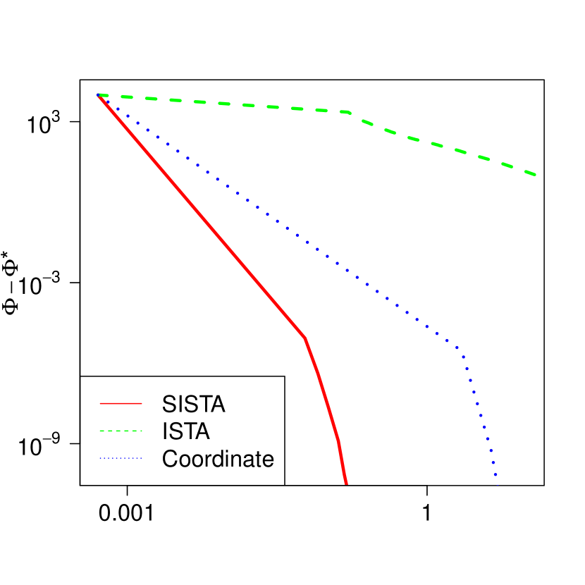
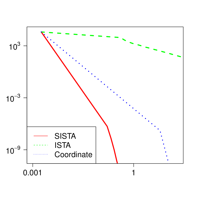
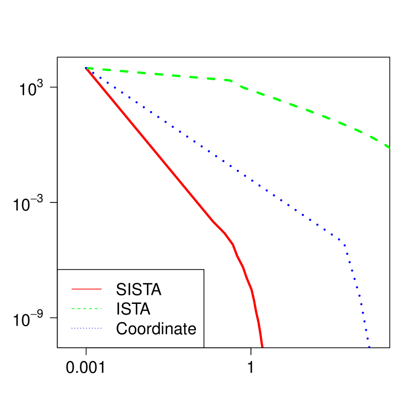
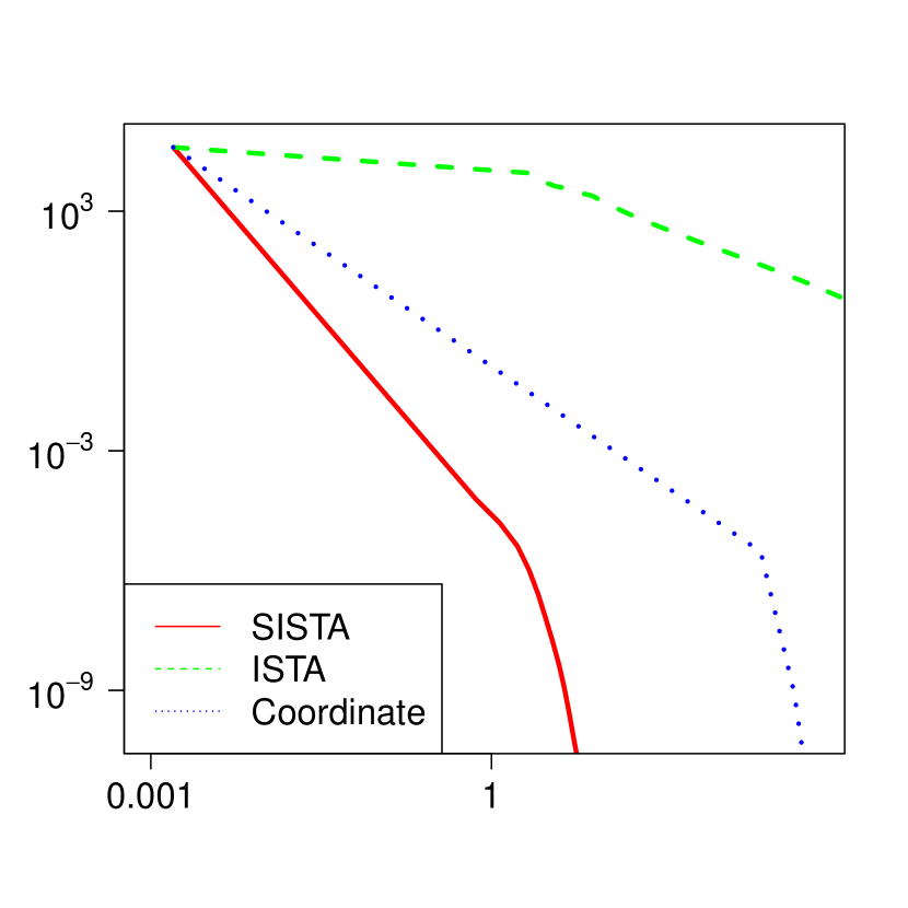
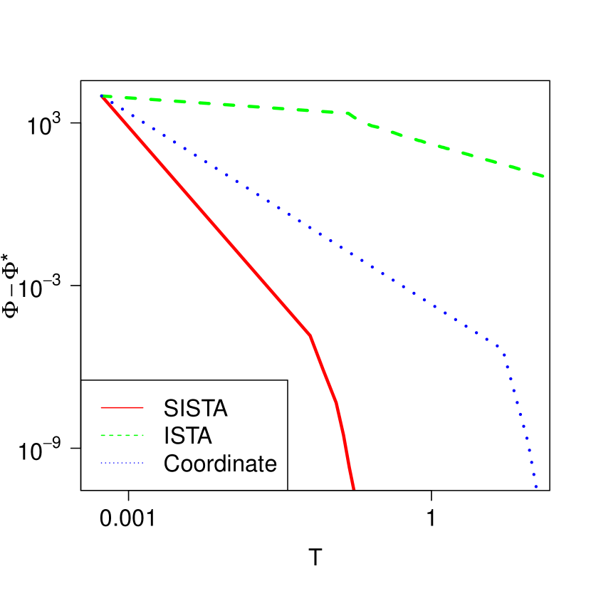
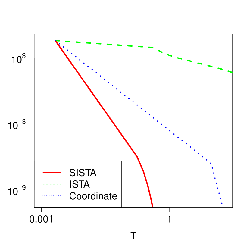
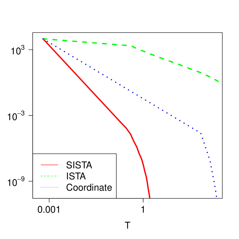
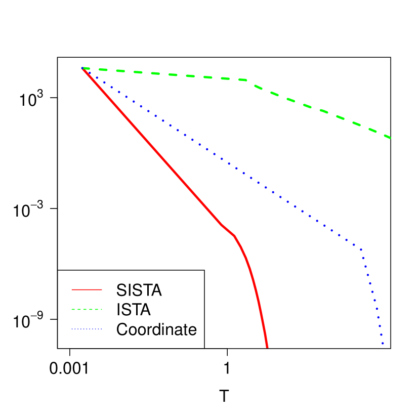
For comparability, the three methods are run using the same initial estimate of the variables, in practice by setting them all to be zero. We can see from figure 1 that SISTA runs an order of magnitude faster than the two pure methods it is a hybrid of. The ISTA method has two major drawbacks compared to the other two. First, a proper initialization of $u,v$ is crucial to ensure a quick convergence of gradient based approaches. Second, a step size has to be set for $u,v$ in addition to $\beta$, which adds extra complexities to the algorithm as they do not necessarily have the same scale as $\beta$. The limitations of coordinate descent are also straightforward to see. As the dimensionality of $\beta$ increases, which is common in practical applications, the cost of coordinate descent increases dramatically, since the algorithm needs to evaluate the gradient after each component’s update, which is time-intensive.

4. Application to migration flows

4.1. Literature

Our goal in this section is to predict migration flows between countries. In this application, $\hat{\pi}_{ij}$ is the probability that a migrant drawn from the overall population of migrants has origin country $i$ and destination country $j$.

The recent compilation of country-to-country migration data (see [18] for instance) has initiated a fast growing literature in economics whose aim is to predict bilateral migration flows using measures of dissimilarity between an origin and a destination country (see [3] for a recent critical review). The dissimilarity measures are built to capture various dimensions of attractiveness of a destination country for migrants from a given origin country, which can be classified into two broad classes: those that are constructed using country-specific characteristics such as Examples (a) and (b) in section 2.2 and pairwise measures such as Example (c).

The current literature has only considered a limited number of dissimilarity measures so far – a minimum of five in [2] and up to a maximum of eight in [20]. The considered ones generally include geographic distances, economic gaps, differences in immigration policy, and cultural differences (see [2, 4, 5, 13, 20]). The parameters are estimated using classical non-linear panel data techniques, where the dependent variable is the logarithm of the bilateral migration flow, and the dissimilarity measures act as independent variables. Countries of origin and destination fixed-effects are usually included in the regression to account for the potential bias due to the fact that the attractiveness of a destination country is relative to that of alternative destination countries, the so-called “multilateral resistance.”

However, the relatively small number of dissimilarity measures studied in this literature is in sharp contrast with the fact that countries differ along many dimensions. A recent effort from various organizations including the World Bank Group, the Centre d’Études Prospectives et d’Informations Internationales (CEPII), Freedom House, has greatly increased the range of measures available for countries. Combining these various sources of data enables one to distinguish more than $200$ countries along over $100$ dimensions, significantly augmenting the size of dissimilarity measures from five or eight.

While this offers scope for improvement in the prediction of bilateral migration flows, it also raises the questions of how to select the most relevant measures of dissimilarity and how to estimate their corresponding parameters. The methodology outlined in the previous section contributes to this literature by providing a solution to them.

4.2. Data

Our application requires access to a working dataset containing information about bilateral migration flows. Each unit in our dataset is an origin-destination country pair. We compile the dataset using five different sources, which gives us over 40,000 observations of bilateral migration flows and more than 100 measures of dissimilarity, including nine pairwise measures.

We use data about bilateral migration flows between 1990 and 2000. These data are obtained in two steps. First, we obtain data about migration stocks in 1990 and 2000 from the dataset compiled by [18], which were collected using census records from 226 countries of origin and destination. Second, we follow the literature (e.g. [4]) and calculate bilateral migration flows between 1990 and 2000 as the change in bilateral stocks of migrants between the two decades.

[4] argues that the existence of a social network at destination, defined as the stock of migrants from the same origin, explains the size and the patterns of international migration flows. We follow [4] and use the stock of migrants from origin country $i$ in destination country $j$ in 1990 as a proxy measure of the network of migrants from $i$ in $j$ in 2000.

We obtain the second set of dissimilarity measures using the data compiled by CEPII and documented in [17]. These data cover 223 countries and contain eight pairwise measures of dissimilarity, including the geographic distance between two countries, whether they are contiguous, and whether they have had a colonial link after 1945.

We incorporate three additional sources to append information about country-specific characteristics covering a vast range of topics.

From the World Development Indicators (WDI), compiled by the World Bank, we obtain 73 variables containing information about economic development (GDP, income, unemployment, inflation, human capital), demography, health (life expectancy, access to improved sanitation facilities), and environment (climate, pollution) for 217 countries.

From the Worldwide Governance Indicators (WGI), also compiled by the World Bank, we obtain six variables about the quality of governance: voice and accountability, political stability and absence of violence, government effectiveness, regulatory quality, rule of law, and control of corruption for 213 countries.

Finally, from Freedom in the World Indicators, compiled by the Freedom House organization, we obtain another 15 variables providing information about political rights and civil liberties for 210 countries.

Combining all these variables, we end up with a vector of 94 characteristics for each country. We then construct 94 measures of dissimilarity as in Example (a) in section 2.2.

4.3. Results

We apply SISTA to our working dataset complied in the previous section. Since the current literature uses between five and eight dissimilarity measures, we perform two sets of experiments, where we conduct a grid search of $\gamma$ so that five and eight components are non-zero in the learned $\beta$.

Table 1. Learned $\beta$ with (top) five (bottom) eight non-zero components.

Contiguity Common language Colonial link after WWII (log) Geo. distance Network Improved sanitation facilities, urban Ori.*Dest. Area Ori.*Dest. Life expect. female Ori.*Dest. 1.797 (0.057) 0 1.224 (0.194) -1.540 (0.020) 1.309 (0.178) 0 -0.630 (0.043) 0 2.438 (0.058) 4.412 (0.108) 2.118 (0.431) -1.992 (0.048) 1.633 (0.211) 2.801 (0.318) -0.927 (0.062) 4.202 (0.535)

Note: Standard errors, calculated using 1,000 bootstrapped samples, are in parentheses.

Table 1 shows the learned $\beta$ from the two experiments. The top row indicates that if only five measures of dissimilarity are allowed in the prediction of migration flows, three of the selected ones are used in most papers in this literature: whether two countries are contiguous, logarithm of geographic distance between them, and whether they have had a colonial link after World War II. The fourth one is the network measure introduced in [2]. Moreover, the signs of $\beta_{k}$’s corresponding to these four measures match precisely with previous results. Interestingly, the fifth selected one has never been used. It corresponds to the interaction between the areas of the origin and destination countries. The negative sign of the parameter indicates that migration flows are larger between small (vast) origin countries and vast (resp. small) destination countries compared to origin-destination countries with similar areas.

The second row indicates that if only eight measures of dissimilarity are to be selected, besides the five mentioned above, the three additional ones are: whether two countries share a language spoken by at least nine percent of their respective population, the interaction between the share of urban population that has access to improved sanitation facilities, and the interaction between the female life expectancy at birth in the origin and destination countries. While the first measure has already been used in [20], with its parameter having the same sign as ours, the other two have not appeared in the literature. The parameters for these new measures are positive, indicating that migration flows tend to be larger between countries with similar urban access to improved sanitation facilities and female life expectancy at birth.

5. Conclusion

This paper introduces a new algorithm, which we called SISTA, to learn the transport cost in optimal transport problems. In this type of problems, one needs to optimize simultaneously over the potentials and over the parameters of the cost. As the parameter vector is sparse, we add an $l_{1}$ penalization over the parameters. SISTA alternates between a phase of exact minimization over the transport potentials and a phase of proximal gradient descent over the parameters of the transport cost. We prove its linear convergence and illustrate through numerical experiments its rapid convergence compared to coordinate descent and ISTA. In our application of predicting bilateral migration flows, SISTA allows us to learn which measures of dissimilarity between an origin and a destination country are the most important ones. Our approach reveals that dissimilarities between origin and destination countries in terms of area, female life expectancy, and urban access to improved sanitation facilities, are critical predictors of bilateral migrations flows that have been absent from this literature.

Our method applies to a broad range of problems in quantitative social sciences. We present an application to the prediction of bilateral migration flows using country-specific characteristics and pairwise measures of dissimilarity between countries. The same technique could be applied to predicting bilateral trade flows, the matching of workers to jobs, men to women, children to schools, etc. In all these applications, there exists a long list of attributes/characteristics upon which measures of dissimilarity between countries of origin and countries of destination, men and women, workers and jobs can be constructed and could explain flows or matches. Our approach allows one to select those that matter the most.

More generally, the idea underlying the SISTA algorithm is broadly applicable. In many other optimization problems, it may be worthwile using hybrid methods combining the strengths of several existing descent methods. As exemplified by SISTA, the hybrid version can be much more efficient than the methods it combines.

References

- [1] Beck, A., & Teboulle, M. (2009). A fast iterative shrinkage-thresholding algorithm for linear inverse problems. SIAM Journal on Imaging Sciences, 2(1), 183–202.
- [2] Beine, M., & Parsons, C. (2015). Climatic factors as determinants of international migration. The Scandinavian Journal of Economics, 117(2), 723–767.
- [3] Beine, M., Bertoli, S., & Fernández-Huertas Moraga, J. (2016). A practitioners’ guide to gravity models of international migration. The World Economy, 39(4), 496–512.
- [4] Beine, M. (2016). The role of networks for migration flows: an update. International Journal of manpower.
- [5] Belot, M., & Ederveen, S. (2012). Cultural barriers in migration between OECD countries. Journal of Population Economics, 25(3), 1077–1105.
- [6] Benamou, J. D., Carlier, G., Cuturi, M., Nenna, L., & Peyré, G. (2015). Iterative Bregman projections for regularized transportation problems. SIAM Journal on Scientific Computing, 37(2), A1111–A1138.
- [7] Cuturi, M. (2013). Sinkhorn distances: Lightspeed computation of optimal transport. In Advances in Neural Information Processing Systems (pp. 2292–2300).
- [8] Cuturi, M., & Avis, D. (2014). Ground metric learning. The Journal of Machine Learning Research, 15(1), 533–564.
- [9] Dupuy, A., & Galichon, A. (2014). Personality traits and the marriage market. Journal of Political Economy, 122(6), 1271–1319.
- [10] Dupuy, A., Galichon, A., & Sun, Y. (2019). Estimating matching affinity matrices under low-rank constraints. Information and Inference: A Journal of the IMA, 8(4), 677–689.
- [11] Galichon, A. (2016). Optimal Transport Methods in Economics. Princeton University Press.
- [12] Galichon, A., & Salanié, B. (2015). Cupid invisible hand: Social surplus and identification in matching models. Available at SSRN 1804623.
- [13] Grogger, J., & Hanson, G. H. (2011). Income maximization and the selection and sorting of international migrants. Journal of Development Economics, 95(1), 42–57.
- [14] Huang, G., Guo, C., Kusner, M. J., Sun, Y., Sha, F., & Weinberger, K. Q. (2016). Supervised word mover’s distance. In Advances in Neural Information Processing Systems (pp. 4862–4870).
- [15] Kulis, B. (2013). Metric learning: A survey. Foundations and Trends in Machine Learning, 5(4), 287–364.
- [16] Idel, M. (2016). A review of matrix scaling and Sinkhorn’s normal form for matrices and positive maps. arXiv preprint arXiv:1609.06349.
- [17] Mayer, T., & Zignago, S. (2011). Notes on CEPII distances measures: The GeoDist database.
- [18] Özden, Ç., Parsons, C. R., Schiff, M., & Walmsley, T. L. (2011). Where on earth is everybody? The evolution of global bilateral migration 1960-2000. The World Bank Economic Review, 25(1), 12–56.
- [19] Peyré, G., & Cuturi, M. (2019). Computational optimal transport. Foundations and Trends in Machine Learning, 11(5–6), 355–607.
- [20] Ramos, R., & Suriñach, J. (2017). A gravity model of migration between the ENC and the EU. Journal of Economic and Social Geography, 108(1), 21–35.
- [21] Santambrogio, F. (2015). Optimal Transport for Applied Mathematicians. Birkhäuser.
- [22] Villani, C. (2003). Topics in Optimal Transportation (No. 58). American Mathematical Society.
- [23] Villani, C. (2008). Optimal Transport: Old and New (Vol. 338). Springer Science & Business Media.