Multivariate binary probability distribution in the Grassmann formalism

Abstract

We propose a probability distribution for multivariate binary random variables. For this purpose, we use the Grassmann number, an anti-commuting number. In our model, the partition function, the central moment, and the marginal and conditional distributions are expressed analytically by the matrix of the parameters analogous to the covariance matrix in the multivariate Gaussian distribution. That is, summation over all possible states is not necessary for obtaining the partition function and various expected values, which is a problem with the conventional multivariate Bernoulli distribution. The proposed model has many similarities to the multivariate Gaussian distribution. For example, the marginal and conditional distributions are expressed by the parameter matrix and its inverse matrix, respectively. That is, the inverse matrix expresses a sort of partial correlation. Analytical expressions for the marginal and conditional distributions are also useful in generating random numbers for multivariate binary variables. Hence, we validated the proposed method using synthetic datasets. We observed that the sampling distributions of various statistics are consistent with the theoretical predictions and estimates are consistent and asymptotically normal.

I Introduction

The multivariate binary probability distribution is a model for multivariate binary random variables. This model is used in many applications such as modeling the behavior of magnets in statistical physics Ising (1925), building statistical models in computer vision Geman and Geman (1984) and social network analysis. In the terminology of the graphical model, the multivariate binary probability distribution is a kind of Markov random fields. This model is essentially the same as the Ising model in statistical physics, and which is also called the Boltzmann machine in the field of machine learning research Ackley et al. (1985). Recent applications of this model include the study in detecting statistical dependence in the voting pattern from senate voting records data Banerjee et al. (2008) and the study of cooperative mutations in the Human Immunodeficiency Virus (HIV) Xue et al. (2012).

Existing methods of multivariate binary probability distribution encode a binary variable as a dummy variable that takes discrete values in $\{0,1\}$ or $\{-1,1\}$, which is called the multivariate Bernoulli distribution or the Ising model. However, such discrete coding prevents us from analytical calculations. For example, the marginal and conditional distributions are no longer in the same form as the original joint distribution. Furthermore, a problem also arises from the viewpoint of computational complexity. In the existing method of the multivariate binary probability distribution, we have to sum over all possible states to calculate the partition function and various expected values, however, in a binary system, the number of possible states exponentially increases as the number of variables increases. In other words, the computation of the partition function and expected values is $\mathrm{NP}$-hard, which causes difficulties with parameter estimation. In fact, the maximum likelihood estimation of model parameters by using a gradient-based method requires the calculation of various expected values, then, the application of such a usual estimation procedure becomes difficult when the number of variables is large. One way of dealing with parameter estimation is to approximate the expected values by Gibbs sampling, a Markov chain Monte Carlo simulation, but this method is computationally demanding and time-consuming. Another way is to approximate the likelihood function to a more tractable functional form. That is the variational inference Wainwright and Jordan (2008), the pseudo-likelihood and the composition likelihood methods Höfling and Tibshirani (2009); Ravikumar et al. (2010); Xue et al. (2012), where methods for estimating the sparse structure of a graph are proposed through the use of $L_{1}$ and non-concave regularizations. However, the multivariate Bernoulli distribution has not been widely used in application compared to the multivariate Gaussian distribution, whose partition function can be analytically computed and is widely used in various fields such as natural language processinig Manning and Schütze (1999), image analysis Woods (1978); Hassner and Sklansky (1980); Geman and Geman (1984) and spatial statistics RIPLEY (1981).

In this paper, we propose a probability distribution that models multivariate binary variables. The difficulty with the existing method of the multivariate binary probability distribution stems from the fact that binary variables are represented by discrete dummy variables, which complicates analytical calculations due to summation over states. Using the Grassmann variable, an anti-commuting number, we rewrite the summation over all possible states by integral of the Grassmann variable. The resulting model resolves the problem in the conventional multivariate Bernoulli distribution that summation over states can not be calculated analytically.

This paper is organized as follows. In Sec. II, we propose a method for the multivariate binary probability distribution using the Grassmann variables. Various properties of our distribution, such as the marginal and conditional distributions and correlatedness and statistical independence are investigated. In Sec. III, we validate our method numerically using synthetic datasets of correlated binary variables. The consistency and asymptotic normality of the sampling distribution of various statistics and estimates are investigated. Sec. IV is devoted to conclusions. We use popular notation in matrix theory. For a $p\times p$ matrix $A$, $A[\eta]$ denotes the principal submatrix of $A$ with rows and columns out of a subset $\eta\subseteq\{1,2,...,p\}$.

II Proposed method

The multivariate Bernoulli distribution is a probability distribution for binary random variables, where the $p$-dimensional binary variables are encoded by the dummy variables taking $x_{i}\in\{0,1\},\;\;i\in P\equiv\{1,2,\dots,p\}$. Usually, the joint distribution of the multivariate Bernoulli distribution is expressed as the exponential function of the quadratic form in the dummy variables Wainwright and Jordan (2008); Dai et al. (2013),

$$p(x_{P})=\frac{1}{Z}\exp\biggl{\{}\sum_{i=1}^{P}b_{i}\,x_{i}+\sum_{i,\,j=1}^{P}x_{i}\,w_{ij}\,x_{j}\biggr{\}},$$ (1)

where $b_{i}$ and $w_{ij}$ are called the bias and weight terms, and the exponent is called the energy function. $Z$ is the partition function that ensures that the distribution sums to one. In the conventional multivariate Bernoulli distribution, various quantities such as the partition function and expected values are computed by summation over all possible states. For example, the expected value of the random variable $x_{i}$ is expressed as the following summation,

$$\mathrm{E}[x_{i}]= \sum_{x_{P}\in\{0,1\}^{p}}x_{i}\,p(x_{P}),$$

$$= \biggl{[}\,\sum_{x_{1}\in\{0,1\}}\sum_{x_{2}\in\{0,1\}}\cdots\sum_{x_{p}\in\{0,1\}}\,\biggr{]}x_{i}\,p(x_{1},x_{2},\dots,x_{p}).$$ (2)

However, for the multivariate binary variables, the number of possible states increases exponentially as the dimension of the variable $p$ increases. Then, performing the summation over states in the expected value becomes difficult even numerically. Furthermore, there exists a difficulty with the conventional multivariate Bernoulli distribution that the marginal and conditional distributions do not follow the multivariate Bernoulli distribution. In fact, the marginal distribution $p(x_{R})$ for indices $R=P\setminus M$, in which the variables with the indices $M\subseteq P$ are marginalized out,

$$p(x_{R})=\sum_{x_{M}}p(x_{R},x_{M}),$$ (3)

is no longer in the same form as the original expression of Eq. (1). Then, it is difficult to interpret the model parameters, while in the multivariate Gaussian distribution the covariance matrix and its inverse matrix can be interpreted as indirect and direct correlations. We try to resolve these difficulties by introducing the Grassmann number, an anti-commuting number. We express the system by a pair of Grassmann variables $\theta$, $\bar{\theta}$, instead of the dummy variable $x$. By expressing the summation over states as an integral of the Grassmann variables, we expect that the partition function and various expected values can be expressed analytically.

II.1 Univariate binary probability distribution

First, we explain our idea with the simplest example of the univariate binary probability distribution. In the conventional Bernoulli distribution, the normalization condition of the probability distribution and expected values of the random variable are computed by summation over all possible states of the dummy variable $x\in\{0,1\}$:

$$\sum_{x}p(x)= 1,$$

$$\mathrm{E}[x]= \sum_{x}x\,p(x)=p(x=1).$$ (4)

On the other hand, our formalism introduces a pair of Grassmann variables $\theta$ and $\bar{\theta}$ Peskin and Schroeder (1995), anti-commuting numbers, corresponding to the dummy variable. These variables obey the following anti-commuting relations:

$$\{\theta,\bar{\theta}\}\equiv \;\theta\bar{\theta}+\bar{\theta}\theta=0,$$

$$\theta^{2}= \;\bar{\theta}^{2}=0.$$ (5)

Then, we assume that instead of the summation described above expected values can be obtained by integration of the Grassmann function defined by

$$e^{H(\bar{\theta},\theta)}= \;\exp\Bigl{\{}\bar{\theta}\,\Lambda\,\theta-\log Z(\Lambda)\Bigr{\}},$$

$$= \;\frac{1}{Z(\Lambda)}\;e^{\bar{\theta}\Lambda\theta},$$ (6)

where $\Lambda$ is a parameter of the model, and $Z(\Lambda)$ is the partition function, the normalization constant that ensures that the distribution sums to one. We hereafter refer to the exponent of the Grassmann function as Hamiltonian $H(\bar{\theta},\theta)$. In the above equation, we have adopted the quadratic form in the Grassmann variables as a Hamiltonian. The partition function is calculated by integration of the Grassmann variables as follows:

$$Z(\Lambda)= \int d\theta d\bar{\theta}\,e^{\bar{\theta}\Lambda\theta},$$

$$= \Lambda\equiv\frac{1}{\Sigma},$$ (7)

where we have adopted the following sign convention of the Grassmann integral:

$$\int d\theta d\bar{\theta}\,\bar{\theta}\theta=1.$$ (8)

Furthermore, we assume that the expected value of the dummy variable $x$, which corresponds to the probability of $p(x=1)$, is calculated by the expected value of the product of the Grassmann variable $(\bar{\theta}\theta)$ as follows:

$$\mathrm{E}[x]=\;p(x=1)= \int d\theta d\bar{\theta}\,(\bar{\theta}\theta)\,e^{H(\bar{\theta},\theta)},$$

$$= \;\frac{1}{\Lambda}\int d\theta d\bar{\theta}\,(\bar{\theta}\theta)\,e^{\bar{\theta}\Lambda\theta},$$

$$= \;\frac{1}{\Lambda}\equiv\Sigma.$$ (9)

Thus, we see that the parameter $\Sigma$ can be interpreted as the mean parameter of the probability distribution. In the same way, we assume that in our formalism the probability $p(x=0)$ is calculated by the expected value of the Grassmann variable $(1-\bar{\theta}\theta)$,

$$p(x=0)= \int d\theta d\bar{\theta}\,(1-\bar{\theta}\theta)\,e^{H(\bar{\theta},\theta)},$$

$$= 1-\Sigma,$$ (10)

which is an analogy from the summation $p(x=0)=\sum_{x}(1-x)\,p(x)$. The central moment of higher order can be derived consistently by the following prescription. Since the Grassmann variable with higher order becomes zero, we first summarize the polynomials for the dummy variable using the identity, $x^{k}=x,\;k\in\{1,2,\dots\}$:

$$\mathrm{E}\bigl{[}(x-\mu)^{k}\bigr{]}=\,\mathrm{E}[x]\,\sum_{l=0}^{k-1}\binom{k}{l}\,(-\mu)^{l}+(-\mu)^{k}.$$ (11)

Then, the Grassmann integral for the above expression gives consistent results. Therefore, our formalism successfully reproduces the univariate Bernoulli distribution.

II.2 Bivariate binary probability distribution

The same idea as the previous subsection is applicable to the bivariate binary probability distribution. We introduce a pair of Grassmann vectors $\theta=(\theta_{1},\theta_{2})^{T}$, $\bar{\theta}=(\bar{\theta}_{1},\bar{\theta}_{2})^{T}$ corresponding to the dummy variables $x_{1}$, $x_{2}$. Again, we assume that the expected value by summation over states can be calculated by integration of the following exponential function of the Grassmann variables,

$$e^{H(\bar{\theta},\theta)}=\frac{1}{Z(\Lambda)}\,e^{\theta^{\dagger}\Lambda\theta},$$ (12)

where $\theta^{\dagger}$ denotes the transpose of the Grassmann vector $\bar{\theta}$, $\theta^{\dagger}\equiv\bar{\theta}^{T}$, and $\Lambda=\Sigma^{-1}$ is a matrix of model parameters analogous to the precision and covariance matrices in the bivariate Gaussian distribution,

$$\Lambda=\begin{bmatrix}\Lambda_{11}&\Lambda_{12}\\ \Lambda_{21}&\Lambda_{22}\end{bmatrix}=\Sigma^{-1}=\begin{bmatrix}\Sigma_{11}&\Sigma_{12}\\ \Sigma_{21}&\Sigma_{22}\end{bmatrix}^{-1}.$$ (13)

We adopt the following sign convention of the Grassmann integral:

$$\int d\theta_{1}d\bar{\theta}_{1}\,d\theta_{2}d\bar{\theta}_{2}\,\theta_{1}\bar{\theta}_{1}\,\theta_{2}\bar{\theta}_{2}=1.$$ (14)

By performing the Grassmann integral, the partition function is expressed by the determinant of the matrix $\Lambda$,

$$Z(\Lambda)= \int d\theta_{1}d\bar{\theta}_{1}d\theta_{2}d\bar{\theta}_{2}\,e^{\theta^{\dagger}\Lambda\theta},$$

$$= \det\Lambda.$$ (15)

We first discuss the joint distribution. In the conventional bivariate Bernoulli distribution, the co-occurrence probability can be rewritten as an expected value of the dummy variables,

$$p(x_{1}=1,x_{2}=1)= \sum_{x_{1},x_{2}}x_{1}x_{2}\,p(x_{1},x_{2}),$$

$$= \;\mathrm{E}[x_{1}\,x_{2}].$$ (16)

In our formalism, we assume that the above summation over states is expressed by the Grassmann integral. In fact, the co-occurrence probability $p(x_{1}=1,x_{2}=1)$ is calculated as

$$p(x_{1}=1,x_{2}=1)= \frac{1}{\det\Lambda}\int d\theta_{1}d\bar{\theta}_{1}d\theta_{2}d\bar{\theta}_{2}\,(\bar{\theta}_{1}\theta_{1})(\bar{\theta}_{2}\theta_{2})\,e^{\theta^{\dagger}\Lambda\theta},$$

$$= \frac{1}{\det\Lambda}.$$ (17)

In the same way, the joint probabilities of the remaining states are calculated as

$$p(x_{1}=1,x_{2}=0)= \;\frac{\Lambda_{22}-1}{\det\Lambda},$$ (18)

$$p(x_{1}=0,x_{2}=1)= \;\frac{\Lambda_{11}-1}{\det\Lambda},$$ (19)

$$p(x_{1}=0,x_{2}=0)= \;\frac{\det(\Lambda-I)}{\det\Lambda},$$ (20)

where $I$ is the identity matrix. The above expressions for the joint distribution can also be interpreted as all of the principal minors of the matrix $\Lambda-I$ divided by $\det\Lambda$. In terms of $\Sigma$, the joint probabilities are summarized as

$$p(x_{1},x_{2})=\det\begin{bmatrix}\Sigma_{11}^{x_{1}}(1-\Sigma_{11})^{1-x_{1}}&(-1)^{1-x_{2}}\Sigma_{12}\\ (-1)^{1-x_{1}}\Sigma_{21}&\Sigma_{22}^{x_{2}}(1-\Sigma_{22})^{1-x_{2}}\end{bmatrix}.$$ (21)

Next, we turn to the marginal distribution. In the conventional bivariate Bernoulli distribution, marginalization of the variable $x_{2}$ is taken by the summation of the dummy variable:

$$p(x_{1})=\sum_{x_{2}}p(x_{1},x_{2}).$$ (22)

Again, we assume that the above marginalization can be performed by the integration of the Grassmann variables $\theta_{2}$ and $\bar{\theta_{2}}$, which is calculated by completing the square and the shift of the integral variables as

$$\int d\theta_{2}d\bar{\theta}_{2}\,e^{H(\bar{\theta},\theta)}= \frac{1}{\det\Lambda}\int d\theta_{2}d\bar{\theta}_{2}\exp\Bigl{\{}\theta^{\dagger}\Lambda\theta\Bigr{\}},$$

$$= \frac{1}{\det\Lambda}\int d\theta_{2}d\bar{\theta}_{2}\exp\Bigl{\{}\bar{\theta}_{1}(\Lambda_{11}-\Lambda_{12}\Lambda_{22}^{-1}\Lambda_{21})\theta_{1}$$

$$\hskip 102.43008pt+(\bar{\theta}_{2}+\bar{\theta}_{1}\Lambda_{12}\Lambda_{22}^{-1})\Lambda_{22}(\theta_{2}+\Lambda_{22}^{-1}\Lambda_{21}\theta_{1})\Bigr{\}},$$

$$= \frac{\Lambda_{22}}{\det\Lambda}\exp\Bigl{\{}\bar{\theta}_{1}(\Lambda_{11}-\Lambda_{12}\Lambda_{22}^{-1}\Lambda_{21})\theta_{1}\Bigr{\}},$$

$$\equiv \;e^{H(\bar{\theta}_{1},\theta_{1})}.$$ (23)

Here, we shall call the resulting Hamiltonian $H(\bar{\theta}_{1},\theta_{1})$ the marginal Hamiltonian. From the above expression, we can read that the marginal distribution still follows the same form as the original joint distribution and the parameter of the resulting distribution is the Schur complement of the matrix $\Lambda$. In terms of $\Sigma$, the marginal distribution is simply expressed by a principal submatrix of $\Sigma$,

$$e^{H(\bar{\theta}_{1},\theta_{1})}=\Sigma_{11}\,e^{\bar{\theta}_{1}\Sigma_{11}^{-1}\theta_{1}}.$$ (24)

Therefore, the diagonal elements of the parameter matrix $\Sigma$ can be interpreted as the mean parameters of the marginal distributions.

Here, we discuss the correlation, covariance and statistical independence of the variables. From an analogy to the bivariate Bernoulli distribution, the covariance between $x_{1}$ and $x_{2}$ can be calculated as a moment about the mean as

$$\mathrm{Cov}[x_{1}\,x_{2}]= \;\mathrm{E}[(x_{1}-\mu_{1})(x_{2}-\mu_{2})],$$

$$= \;\frac{1}{\det\Lambda}\int d\theta_{1}d\bar{\theta}_{1}d\theta_{2}d\bar{\theta}_{2}\,(\bar{\theta}_{1}\theta_{1}-\mu_{1})(\bar{\theta}_{2}\theta_{2}-\mu_{2})\,e^{\theta^{\dagger}\Lambda\theta},$$

$$= -\Sigma_{12}\Sigma_{21},$$ (25)

where $\mu_{i}\equiv\mathrm{E}[x_{i}]=\Sigma_{ii}$ is the mean parameter. Therefore, the product of the off-diagonal terms can be interpreted as the covariance of the variables. Here, we notice that the expression for the joint distribution, Eq. (21), can be transformed to

$$p(x_{1},x_{2})= p(x_{1})p(x_{2})-(-1)^{x_{1}+x_{2}}\Sigma_{12}\Sigma_{21}.$$ (26)

When we define correlation of binary variables by the Pearson correlation coefficient expressed as

$$\rho_{12}\equiv \frac{\mathrm{Cov}[x_{1}\,x_{2}]}{\sqrt{\mathrm{Cov}[x_{1}\,x_{1}]\mathrm{Cov}[x_{2}\,x_{2}]}},$$

$$= \frac{-\Sigma_{12}\Sigma_{21}}{\sqrt{\Sigma_{11}(1-\Sigma_{11})\Sigma_{22}(1-\Sigma_{22})}},$$ (27)

the statistical independence between $x_{1}$ and $x_{2}$ is equivalent to $\Sigma_{12}\Sigma_{21}\propto\rho_{12}=0$. Therefore, in our model, the uncorrelatedness between variables is equivalent to statistical independence as in the case of the Gaussian distribution:

$$\rho_{12}=0,\;\;\Leftrightarrow\;\;p(x_{1},x_{2})=p(x_{1})p(x_{2}).$$ (28)

Lastly, we discuss the conditional distribution. In the conventional Bernoulli distribution, the conditioning on the observation $x_{2}=1$ is expressed by the summation over the dummy variable using the Bayes’ theorem:

$$p(x_{1}|x_{2}=1)= \frac{p(x_{1},x_{2}=1)}{p(x_{2}=1)},$$

$$= \frac{\sum_{x_{2}}x_{2}\,p(x_{1},x_{2})}{p(x_{2}=1)}.$$ (29)

Again, we rewrite the above summation by the Grassmann integral. Then, the Hamiltonian corresponding to the conditional distribution, which we call the conditional Hamiltonian $H(\bar{\theta}_{1},\theta_{1}|x_{2}=1)$, is calculated as

$$e^{H(\bar{\theta}_{1},\theta_{1}|x_{2}=1)}\equiv \;\frac{1}{p(x_{2}=1)}\int d\theta_{2}d\bar{\theta}_{2}\,(\bar{\theta}_{2}\theta_{2})\,e^{H(\bar{\theta},\theta)},$$

$$= \;\frac{1}{p(x_{2}=1)}\frac{1}{\det\Lambda}\int d\theta_{2}d\bar{\theta}_{2}\,(\bar{\theta}_{2}\theta_{2})\,e^{\bar{\theta}\Lambda\theta},$$

$$= \;\frac{1}{\Lambda_{11}}\;e^{\bar{\theta}_{1}\Lambda_{11}\theta_{1}}.$$ (30)

Therefore, the conditional distribution given $x_{2}=1$ still follows the same form as the original joint distribution and the model parameter is just a principal submatrix of $\Lambda$. In terms of $\Sigma$, the above conditional distribution is expressed by the Schur complement of $\Sigma$ with respect to $\Sigma_{22}$:

$$e^{H(\bar{\theta}_{1},\theta_{1}|x_{2}=1)}= \,\Sigma_{1|2}\;e^{\bar{\theta}_{1}\Sigma_{1|2}^{-1}\theta_{1}},$$ (31)

$$\Sigma_{1|2}= \,\Sigma_{11}-\Sigma_{12}\Sigma_{22}^{-1}\Sigma_{21}.$$ (32)

In the same way, the conditional Hamiltonian by the observation $x_{2}=0$ is calculated as

$$e^{H(\bar{\theta}_{1},\theta_{1}|x_{2}=0)}\equiv \;\frac{1}{p(x_{2}=0)}\frac{1}{\det\Lambda}\int d\theta_{2}d\bar{\theta}_{2}\,(1-\bar{\theta}_{2}\theta_{2})\,e^{\bar{\theta}\Lambda\theta},$$

$$= \;\frac{\Lambda_{22}-1}{\det\Lambda}\exp\Bigl{\{}\bar{\theta}_{1}\bigl{[}\Lambda_{11}-\Lambda_{12}(\Lambda_{22}-1)^{-1}\Lambda_{21}\bigr{]}\theta_{1}\Bigr{\}}.$$ (33)

Again, the conditional distribution given $x_{2}=0$ still follows the same form as the joint distribution. The meaning of the conditioning is easy to interpret in terms of $\Sigma$. In fact, the mean of the variable $x_{1}$ is shifted by each conditioning as follows:

$$p(x_{1}=1|x_{2}=1)= \;\Sigma_{11}-\Sigma_{12}\Sigma_{22}^{-1}\Sigma_{21},$$ (34)

$$p(x_{1}=1|x_{2}=0)= \;\Sigma_{11}-\Sigma_{12}(\Sigma_{22}-1)^{-1}\Sigma_{21},$$

$$= \;\Sigma_{11}-(-\Sigma_{12})(1-\Sigma_{22})^{-1}\Sigma_{21}.$$ (35)

The conditioning on $x_{2}=1$ is expressed by the partial covariance matrix $\Sigma_{1|2}$ for observing variables with the mean $\Sigma_{22}$ and covariance $-\Sigma_{12}\Sigma_{21}$. On the other hand, the conditioning on $x_{2}=0$ is expressed by the partial covariance matrix for observing variables with the mean and the sign of the correlation are inverted as $1-\Sigma_{22}$ and $-(-\Sigma_{12})\Sigma_{21}$. In other words, the conditional distribution given $x_{2}=0$ is simply expressed by the Schur complement of the following matrix $\tilde{\Sigma}$ with respect to $\tilde{\Sigma}_{22}$,

$$\tilde{\Sigma}\equiv\begin{bmatrix}\Sigma_{11}&-\Sigma_{12}\\ \Sigma_{21}&1-\Sigma_{22}\end{bmatrix}.$$ (36)

II.3 $p$-dimensional binary probability distribution

The procedure in the previous subsections can be extended to $p$-dimensional variables straightforwardly. In this subsection, we just enumerate the results. First, we introduce a pair of $p$-dimensional Grassmann vectors $\theta=(\theta_{1},\theta_{2},\dots,\theta_{p})^{T}$, $\bar{\theta}=(\bar{\theta}_{1},\bar{\theta}_{2},\dots,\bar{\theta}_{p})^{T}$ and the matrix of the parameters with $p\times p$ dimension, $\Lambda=\Sigma^{-1}$. Then, the expected value by summation over states is replaced with the Grassmann integral of the following function,

$$e^{H(\bar{\theta},\theta)}\equiv\frac{1}{\det\Lambda}\,e^{\theta^{\dagger}\Lambda\theta}.$$ (37)

We adopt the following sign convention of the Grassmann integral:

$$\int d\theta_{1}d\bar{\theta}_{1}d\theta_{2}d\bar{\theta}_{2}\cdots d\theta_{p}d\bar{\theta}_{p}\,(\bar{\theta}_{1}\theta_{1})(\bar{\theta}_{2}\theta_{2})\cdots(\bar{\theta}_{p}\theta_{p})=1.$$ (38)

To discuss the joint distribution, we here define index labels for the variables. We write the set of all indices of the $p$-dimensional binary variables as $P\equiv\{1,2,\dots,p\}$. Then, we write the index label for the variables observed as $x_{i}=1$ as $A\subseteq P$, and denote these variables as $x_{A}$. In the same way, we write the index label for the variables observed as $x_{i}=0$ as $B\subseteq P$, and denote these variables as $x_{B}$. Then, without loss of generality, the matrix of the parameters is expressed as a partitioned matrix as follows:

$$\Sigma=\begin{bmatrix}\Sigma_{AA}&\Sigma_{AB}\\ \Sigma_{BA}&\Sigma_{BB}\end{bmatrix}=\Lambda^{-1}=\begin{bmatrix}\Lambda_{AA}&\Lambda_{AB}\\ \Lambda_{BA}&\Lambda_{BB}\end{bmatrix}^{-1}.$$ (39)

Then, the joint distribution is given by

$$p(x_{A}=1,x_{B}=0)= \;\frac{1}{\det\Lambda}\int d\theta_{P}d\bar{\theta}_{P}\,(\bar{\theta}_{A}\theta_{A})(1-\bar{\theta}_{B}\theta_{B})\,e^{\theta^{\dagger}\Lambda\theta},$$

$$\equiv \;\frac{1}{\det\Lambda}\int\biggl{[}\prod_{i=1}^{p}d\theta_{i}d\bar{\theta}_{i}\biggr{]}\biggl{[}\prod_{j\in A}\bar{\theta}_{j}\theta_{j}\biggr{]}\biggl{[}\prod_{k\in B}(1-\bar{\theta}_{k}\theta_{k})\biggr{]}e^{\theta^{\dagger}\Lambda\theta},$$

$$= \;\frac{1}{\det\Lambda}\det(\Lambda_{BB}-I),$$

$$= \;\det\begin{bmatrix}\Sigma_{AA}&-\Sigma_{AB}\\ \Sigma_{BA}&I-\Sigma_{BB}\end{bmatrix},$$ (40)

where $I$ denotes the identity matrix. The above equation indicates that the joint probabilities are expressed by the principal minors of the matrix $\Lambda-I$ divided by $\det\Lambda$.

Next, we turn to the marginal distribution. We write the index labels of the marginalized and the remaining variables as $M$ and $R$. Then, without loss of generality, the model parameters are written by a partitioned matrix as follows:

$$\Sigma=\begin{bmatrix}\Sigma_{RR}&\Sigma_{RM}\\ \Sigma_{MR}&\Sigma_{MM}\end{bmatrix}=\Lambda^{-1}=\begin{bmatrix}\Lambda_{RR}&\Lambda_{RM}\\ \Lambda_{MR}&\Lambda_{MM}\end{bmatrix}^{-1}.$$ (41)

Then, the marginal Hamiltonian $H(\bar{\theta}_{R},\theta_{R})$ is expressed as

$$e^{H(\bar{\theta}_{R},\theta_{R})}\equiv \;\frac{1}{\det\Lambda}\int d\theta_{M}d\bar{\theta}_{M}\,e^{\theta^{\dagger}\Lambda\theta},$$

$$= \;\det\Sigma_{RR}\;e^{\theta_{R}^{\dagger}\Sigma_{RR}^{-1}\theta_{R}},$$ (42)

where

$$\Sigma_{RR}^{-1}= \;\Lambda_{RR}^{(M)},$$

$$\equiv \;\Lambda_{RR}-\Lambda_{RM}\Lambda_{MM}^{-1}\Lambda_{MR}.$$ (43)

The parameter of the marginal Hamiltonian is just a principal submatrix of $\Sigma$ with the same indices of rows and columns. That is, the diagonal and off-diagonal elements of the matrix $\Sigma_{ij}$ denote the mean and the covariance with all the other variables marginalized out. When the product of the off-diagonal elements $-\Sigma_{ij}\Sigma_{ji}$ vanishes the variable $x_{i}$ and $x_{j}$ are unconditionally independent, or marginally independent. The central moment of higher order can also be calculated by the Grassmann integral. For example, the central moment for the variables with the index label $R$ is given by

$$\mu_{R}\equiv \,\mathrm{E}\Bigl{[}(x_{R}-\mu_{R})\Bigr{]},$$

$$= \,\mathrm{E}\biggl{[}\;\prod_{i\in R}(x_{i}-\mu_{i})\biggr{]},$$

$$= \,\frac{1}{\det\Lambda}\int d\theta_{P}d\bar{\theta}_{P}\prod_{i\in R}(\bar{\theta}_{i}\theta_{i}-\mu_{i})\,e^{\theta^{\dagger}\Lambda\theta},$$

$$= \,\det\Bigl{[}\Sigma_{RR}-I_{R}(\mu_{R})\Bigr{]},$$ (44)

where $I_{R}(\mu_{R})$ is a diagonal matrix with the diagonal element given by $\mu_{R}$,

$$I_{R}(\mu_{R})\equiv \;\mathrm{diag}(\mu_{R}),$$

$$= \;\delta_{ij}\,\mu_{i},\hskip 14.22636pt(i,j\in R),$$ (45)

and $\delta_{ij}$ is the Kronecker delta. We write a fourth-order central moment here for future reference:

$$\mu_{iijj}\equiv \,\mathrm{E}\Bigl{[}(x_{i}-\mu_{i})^{2}(x_{j}-\mu_{j})^{2}\Bigr{]},\;\;\;(i\neq j),$$

$$= \,\mathrm{E}\Biggl{[}\Bigl{[}(1-2\mu_{i})x_{i}+\mu_{i}^{2}\Bigr{]}\Bigl{[}(1-2\mu_{j})x_{j}+\mu_{j}^{2}\Bigr{]}\Biggr{]},$$

$$= (1-2\mu_{i})(1-2\mu_{j})(-\Sigma_{ij}\Sigma_{ji})+\mu_{i}(1-\mu_{i})\mu_{j}(1-\mu_{j}).$$ (46)

Then, we discuss the conditional distribution. As in the case of the joint distribution, we write index labels for the variables observed as $x_{i}=1$ and $x_{i}=0$ as $A$ and $B$, and write these variables as $x_{A}$ and $x_{B}$, respectively. We write the union of $A$ and $B$ as $C$, i.e., $x_{C}=(x_{A},x_{B})$. Then, the remaining indices after conditioning are represented by the set difference of these indices $R=P\setminus(A\cup B)\equiv P\setminus C$. Without loss of generality, the matrix of the parameters is expressed as a partitioned matrix as follows:

$$\Sigma= \begin{bmatrix}\Sigma_{RR}&\Sigma_{RC}\\ \Sigma_{CR}&\Sigma_{CC}\end{bmatrix}=\begin{bmatrix}\Sigma_{RR}&\Sigma_{RA}&\Sigma_{RB}\\ \Sigma_{AR}&\Sigma_{AA}&\Sigma_{AB}\\ \Sigma_{BR}&\Sigma_{BA}&\Sigma_{BB}\end{bmatrix},$$ (47)

$$\Lambda= \begin{bmatrix}\Lambda_{RR}&\Lambda_{RC}\\ \Lambda_{CR}&\Lambda_{CC}\end{bmatrix}=\begin{bmatrix}\Lambda_{RR}&\Lambda_{RA}&\Lambda_{RB}\\ \Lambda_{AR}&\Lambda_{AA}&\Lambda_{AB}\\ \Lambda_{BR}&\Lambda_{BA}&\Lambda_{BB}\end{bmatrix}.$$ (48)

The conditional Hamiltonian $H(\bar{\theta}_{R},\theta_{R}|x_{C})$ is given by

$$e^{H(\bar{\theta}_{R},\theta_{R}|x_{C})}= \;\frac{1}{\det\Lambda}\int d\theta_{C}d\bar{\theta}_{C}\,(\bar{\theta}_{A}\theta_{A})(1-\bar{\theta}_{B}\theta_{B})\,e^{\theta^{\dagger}\Lambda\theta},$$

$$= \;\frac{1}{\det\Lambda_{R|C}}\,e^{\theta_{R}^{\dagger}\Lambda_{R|C}\theta_{R}},$$ (49)

where

$$\Lambda_{R|C}= \;\Lambda_{RR}-\Lambda_{RB}\bigl{(}\Lambda_{BB}-I\bigr{)}^{-1}\Lambda_{BR},$$

$$= \Bigl{[}\Sigma_{RR}-\Sigma_{RC}\bigl{[}\Sigma_{CC}-I_{C}(1-x_{C})\bigr{]}^{-1}\Sigma_{CR}\Bigr{]}^{-1},$$ (50)

and $I_{C}(1-x_{C})$ is the diagonal matrix defined by Eq. (45):

$$I_{C}(1-x_{C})\equiv \;\mathrm{diag}(1-x_{C}),$$

$$= \;\delta_{ij}\,(1-x_{i}),\hskip 14.22636pt(i,j\in C),$$ (51)

As in the case of the bivariate variables, we can give an intuitive interpretation of the parameters of the conditional distribution. In fact, the matrix $\Lambda_{R|C}$ can be rewritten by the Schur complement of the following matrix $\tilde{\Sigma}$ with respect to the principal submatrix $\tilde{\Sigma}_{CC}$,

$$\Lambda_{R|C}= \;\tilde{\Sigma}_{R|C}^{-1},$$

$$= \;\bigl{[}\Sigma_{RR}-\tilde{\Sigma}_{RC}\tilde{\Sigma}_{CC}^{-1}\Sigma_{CR}\bigr{]}^{-1},$$

$$= \;\tilde{\Lambda}_{RR},$$ (52)

where

$$\tilde{\Sigma}\equiv \begin{bmatrix}\Sigma_{RR}&\tilde{\Sigma}_{RC}\\ \Sigma_{CR}&\tilde{\Sigma}_{CC}\end{bmatrix}\equiv\begin{bmatrix}\Sigma_{RR}&\Sigma_{RA}&-\Sigma_{RB}\\ \Sigma_{AR}&\Sigma_{AA}&-\Sigma_{AB}\\ \Sigma_{BR}&\Sigma_{BA}&I-\Sigma_{BB}\end{bmatrix}\equiv\tilde{\Lambda}^{-1},$$

$$= \begin{bmatrix}\Lambda_{RR}-\Lambda_{RB}(\Lambda_{BB}-I)^{-1}\Lambda_{BR}&\Lambda_{RA}-\Lambda_{RB}(\Lambda_{BB}-I)^{-1}\Lambda_{BA}&-\Lambda_{RB}(\Lambda_{BB}-I)^{-1}\\ \Lambda_{AR}-\Lambda_{AB}(\Lambda_{BB}-I)^{-1}\Lambda_{BR}&\Lambda_{AA}-\Lambda_{AB}(\Lambda_{BB}-I)^{-1}\Lambda_{BA}&-\Lambda_{AB}(\Lambda_{BB}-I)^{-1}\\ (\Lambda_{BB}-I)^{-1}\Lambda_{BR}&(\Lambda_{BB}-I)^{-1}\Lambda_{BA}&\Lambda_{BB}(\Lambda_{BB}-I)^{-1}\end{bmatrix}^{-1}.$$ (53)

The matrix $\tilde{\Sigma}$ corresponds to the original matrix $\Sigma$ with the mean and sign of the covariance parameters for the variables $x_{B}$ inverted as $I-\Sigma_{BB}$ and $(-\Sigma_{RB},-\Sigma_{AB})$, respectively. In other words, observing the dummy variable $x_{i}$ as $x_{i}=0$ is equivalent to observing the dummy variable $\tilde{x}_{i}$ with the dummy coding inverted as $\tilde{x}_{i}=1$. Therefore, our formalism is a symmetric formalism that does not depend on how to encode binary variables.

The matrix $\Lambda$ can also be interpreted intuitively. From Eq. (50), we see that the diagonal element of $\Lambda$ expresses the inverse of the mean conditioned on all the other variables observed as $x_{A}=1$. Furthermore, the off-diagonal elements can be interpreted as the partial correlation, similar to the multivariate Gaussian distribution. Here, we consider the conditional distribution of $x_{R}=(x_{1},x_{2})$ given $x_{A}=1,\;A=P\setminus\{1,2\}$. The corresponding conditional Hamiltonian is given by

$$e^{H(\bar{\theta}_{R},\theta_{R}|x_{A})}= \;\frac{1}{\det\Lambda_{RR}}\,e^{\theta_{R}^{\dagger}\Lambda_{RR}\theta_{R}},$$

$$= \;\det\Sigma_{R|A}\;e^{\theta_{R}^{\dagger}\Sigma_{R|A}^{-1}\theta_{R}},$$ (54)

where

$$\Sigma_{R|A}= \begin{bmatrix}\Sigma_{11|A}&\Sigma_{12|A}\\ \Sigma_{21|A}&\Sigma_{22|A}\end{bmatrix}=\Lambda_{RR}^{-1}=\frac{1}{\det\Lambda_{RR}}\begin{bmatrix}\Lambda_{22}&-\Lambda_{12}\\ -\Lambda_{21}&\Lambda_{11}\end{bmatrix}.$$ (55)

Then, the correlation between $x_{1}$ and $x_{2}$ for the conditional distribution, i.e., the partial correlation $\rho_{12|A}$, is expressed by the product of the off-diagonal elements of $\Lambda_{RR}$:

$$\rho_{12|A}= \;\frac{-\Sigma_{12|A}\Sigma_{21|A}}{\sqrt{\Sigma_{11|A}(1-\Sigma_{11|A})\Sigma_{22|A}(1-\Sigma_{22|A})}},$$

$$= \;\frac{-\Lambda_{12}\Lambda_{21}}{\sqrt{\Lambda_{22}(\det\Lambda_{RR}-\Lambda_{22})\Lambda_{11}(\det\Lambda_{RR}-\Lambda_{11})}}.$$ (56)

Therefore, $\Lambda$ can be interpreted as the partial correlation with all the other variables observed as $x_{A}=1$. When the partial correlation conditioned on $x_{A}=1$ vanishes the variables $x_{1}$ and $x_{2}$ are conditionally independent:

$$\rho_{ij|A}=0,\;\;\Leftrightarrow\;\;p(x_{i},x_{j}|x_{A}=1)=p(x_{i}|x_{A}=1)\,p(x_{j}|x_{A}=1).$$ (57)

The partial correlation for the general conditioning $x_{C}=(x_{A}=1,x_{B}=0)$ other than $x_{A}=1$ can also be interpreted in the same way. In this case, we first define the matrix $\tilde{\Sigma}$ in which the dummy coding of the variables observed as $x_{B}=0$ is inverted to $\tilde{x}_{B}=1$ as in Eq. (53). Then the product of the off-diagonal elements of the inverse matrix $\tilde{\Lambda}=\tilde{\Sigma}^{-1}$ expresses the magnitude of the partial correlation under that conditioning. The partial correlation for the general conditioning is given by the same expression, Eq. (56), except that $\Lambda$ is replaced by $\tilde{\Lambda}$.

Lastly, we should mention the normalization and positivity of our probability distribution. Since the analytical expression for the partition function is obtained, the normalization of the joint distribution should be satisfied. This can be confirmed from the identity of the principal minors. In fact, the joint probabilities of the $p$-dimensional binary variables are expressed by the principal minors of the matrix $\Lambda-I$ divided by $\det\Lambda$ as shown in Eq. (40). When we notice the identity regarding the summation over all principal minors,

$$\sum_{B\subseteq P}\det(\Lambda_{BB}-I)=\det\Lambda,$$ (58)

we see that the normalization of the joint distribution is satisfied by definition. On the other hand, the positivity that all probabilities of the joint distribution are greater than or equal to zero does not necessarily true in general. Expressed in the terminology of linear algebra, the positivity that all joint probabilities must be positive is equivalent to that the matrix $\Lambda-I$ must be a $P_{0}$-matrix, which is an important property in various applications Berman and Plemmons (1994). When the matrix $\Lambda-I$ is a $P$-matrix, the positivity of the marginal and conditional distributions can also be confirmed. The marginal distribution is expressed as the Schur complement of $\Lambda$ as in Eq. (43). In other words, the positivity of the marginal probabilities is expressed as the positivity of the determinants of the Schur complements of each principal submatrix of the following matrix, $(\Lambda-I+I_{P}(\delta_{PM}))[R^{\prime}\cup M]\;\;(R^{\prime}\subseteq R)$, with respect to $\Lambda_{MM}$:

$$\Lambda-I+I_{P}(\delta_{PM})\equiv\begin{bmatrix}\Lambda_{RR}-I&\Lambda_{RM}\\ \Lambda_{MR}&\Lambda_{MM}\end{bmatrix}.$$ (59)

The above matrix is the matrix $\Lambda-I$ plus the identity submatrix $I_{P}(\delta_{PM})$. Since adding an identity submatrix amounts to shifting the real part of the eigenvalues by one, the matrix $\Lambda-I+I_{P}(\delta_{PM})$ and its principal submatrices are still $p$-matrices. From the identity of the determinant of the block matrix, the determinant of the Schur complement of a $P$-matrix is positive, therefore, all of the marginal probabilities are positive. For the conditional probabilities, their positivity is rephrased as the positivity of the determinants of the Schur complements of each principal submatrix $(\Lambda-I)[R^{\prime}\cup B]\;\;(R^{\prime}\subseteq R)$ with respect to $\Lambda_{BB}-I$ as can be seen from Eq. (50). Again, since the determinant of the Schur complement of the $P$-matrix $(\Lambda-I)[R^{\prime}\cup B]$ is positive, all of the conditional probabilities are positive. These properties are in contrast to those of the conventional multivariate Bernoulli distribution. In the multivariate Bernoulli distribution, the partition function is not given analytically but has to be summed numerically over all possible states. On the other hand, the property that all joint probabilities are positive is satisfied by definition because probability distributions are given by the exponential function of the polynomial in the dummy variables as shown in Eq. (1).

III Numerical experiments

In this section, we validate our method numerically. Since the analytical expressions for the marginal and conditional distributions are obtained in our formalism, we can easily generate random numbers for correlated binary variables by repeating Bernoulli trials. Hence, we investigate the sampling distributions of various statistics and estimates using synthetic datasets. Below, we define index labels for the variables used in this section. We denote the set of all indices for $p$-dimensional binary variables as $P\equiv\{1,2,\dots,p\}$. Then, we write the index labels for the variables observed as $x_{i}=1$ and $x_{i}=0$ as $A$ and $B$, and write these variables as $x_{A}$ and $x_{B}$, respectively. We denote a specific realization of the dummy vector as $\delta$, for example, $\delta=(1,0,1,1,0)$ for five-dimensional variables. Generated data are represented by $\mathcal{D}=\{x_{1P},x_{2P},\dots,x_{NP}\}$, where $x_{nP},\;n\in\{1,2,\dots,N\}$, is a $p$-dimensional vector of dummy variables

III.1 Sampling distribution of statistics

Since the covariance structure of our model is determined by the product of off-diagonal elements of the matrix, $-\Sigma_{ij}\Sigma_{ji}$, the parameters $\Sigma_{ij}$ themselves are not fixed uniquely even though we set the mean and covariance by hand. Hence, the remaining parameters of the model $\Sigma_{ij}\;(i<j)$ with a given mean and covariance are determined by maximizing the entropy of the joint distribution $\mathbb{H}(p|\Sigma_{ij})$,

$$\mathbb{H}(p|\Sigma_{ij})=-\sum_{\delta}p(x_{P}=\delta|\Sigma_{ij})\log p(x_{P}=\delta|\Sigma_{ij}),$$ (60)

where the summation has been taken over all possible states. Correlated random numbers for multivariate binary variables can be generated by repeating Bernoulli trials using the analytical expressions for the marginal and conditional distributions. In fact, since the joint distribution can be factorized as $p(x_{1},x_{2},\dots,x_{p})=p(x_{1})p(x_{2}|x_{1})\cdots p(x_{p}|x_{1},x_{2},\dots,x_{p-1})$, we can generate a random number by repeating Bernoulli trials $p$ times from $p(x_{1})$ to $p(x_{p}|x_{1},x_{2},\dots,x_{p-1})$ depending on the previous observations. The dimension of the variables used to generate the synthetic datasets is $p=5$, and the mean parameters are $\mu_{1}=0.77$, $\mu_{2}=0.37$, $\mu_{3}=0.67$, $\mu_{4}=0.42$, $\mu_{5}=0.7$. The correlation coefficients of the variables are $\rho_{12}=-0.03$, $\rho_{13}=0.32$, $\rho_{14}=-0.1$, $\rho_{15}=0.04$, $\rho_{23}=0.004$, $\rho_{24}=0.003$, $\rho_{25}=0.06$, $\rho_{34}=-0.03$, $\rho_{35}=0.05$, $\rho_{45}=-0.19$, where we have defined the correlation coefficient for binary variables by the Pearson correlation coefficient.

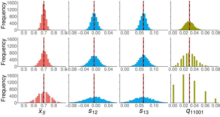
Figure 1: Examples of the sampling distributions of the statistics for the sample mean $\bar{x}_{5}$, unbiased sample covariances $s_{12}$, $s_{13}$, and the empirical joint distribution $q(x_{P}=(1,1,0,0,1))$. The first, second and third rows correspond to the results of the sample sizes $N=500$, $N=200$ and $N=50$, respectively. The trial size, i.e., the number of times the statistics are computed, is $M=5000$. The red solid lines denote the true values and the black dashed lines denote the mean values of the sampling distributions.

Fig. 1 shows the sampling distributions of the statistics for the sample mean and unbiased sample covariance and the empirical joint distribution from the synthetic datasets for different sample sizes $N$. The unbiased sample covariance is defined as

$$s_{ij}\equiv \;\frac{1}{N-1}\sum_{n=1}^{N}(x_{ni}-\bar{x}_{i})(x_{nj}-\bar{x}_{j}),\hskip 14.22636pt(i\neq j),$$ (61)

$$\bar{x}_{i}\equiv \;\frac{1}{N}\sum_{n=1}^{N}x_{ni}.$$ (62)

We observe that the sampling distributions of the statistics are consistent with the following theoretical predictions:

$$\mathrm{E}[\bar{x}_{i}]= \,\mu_{i},$$ (63)

$$\mathrm{Var}[\bar{x}_{i}]= \,\frac{1}{N}\,\mu_{i}\,(1-\mu_{i}),$$ (64)

$$\hskip 99.58464pt\mathrm{E}[s_{ij}]= -\Sigma_{ij}\Sigma_{ji},$$

$$\equiv \;\sigma_{ij},$$ (65)

$$\mathrm{Var}[s_{ij}]= \frac{1}{N}\mu_{iijj}-\frac{(N-2)}{N(N-1)}(\mu_{ij})^{2}+\frac{1}{N(N-1)}\mu_{ii}\,\mu_{jj},$$ (66)

where $\mu_{ii}\equiv\mu_{i}(1-\mu_{i})$ and $\mu_{iijj}$ are the second- and fourth-order central moments,

$$\mathrm{E}[q_{\delta}]= \,\pi_{\delta}(\Sigma),$$ (67)

$$\mathrm{Var}[q_{\delta}]= \,\frac{1}{N}\,\pi_{\delta}(\Sigma)\bigl{[}1-\pi_{\delta}(\Sigma)\bigr{]}.$$ (68)

Although the sampling distribution can be skewed when the sample size is small, it becomes asymptotically normal as the sample size increases, which is consistent with the central limit theorem. These observations, in turn, demonstrate the justification of our method.

III.2 Sampling distribution of estimates

In this subsection, we discuss a method of parameter estimation and the sampling distribution of estimates given observed data. A common method of parameter estimation is the maximum likelihood estimation given observed data $\mathcal{D}$. In our model, the log-likelihood is expressed as

$$l(\Sigma|\mathcal{D})= \sum_{n=1}^{N}\log p(x_{nP}|\Sigma),$$

$$= \,N\sum_{\delta}\frac{n_{\delta}}{N}\log p(x_{P}=\delta|\Sigma),$$

$$\equiv \,N\sum_{\delta}q_{\delta}\log\pi_{\delta}(\Sigma),$$ (69)

where $n_{\delta}$ is the number of times we observed the state as $x_{P}=\delta$, which satisfies $\sum_{\delta}n_{\delta}=N$. In other words, the log-likelihood is expressed as the cross entropy between the empirical joint distribution $q_{\delta}$ and the distribution by the model $\pi_{\delta}(\Sigma)\equiv p(x_{P}=\delta|\Sigma)$.

The maximum likelihood estimation of Eq. (69) by using gradient-based methods is valid when the sample size is large or the number of variable $p$ is small. However, when it is not the case many of the empirical joint probabilities $q_{\delta}$ become zero which causes the difficulty that the corresponding joint distribution by the model $\pi_{\delta}(\Sigma)$ can take a negative value during parameter estimation. Hence, in this paper, we use the maximum a posterior ($\mathrm{MAP}$) estimation instead of the maximum likelihood estimation. We assign the Dirichlet distribution for a prior probability on the joint distribution by the model $\pi_{\delta}(\Sigma)\equiv p(x_{P}=\delta|\Sigma)$ so that the joint probabilities of all states are always positive,

$$p(\Sigma|\mathcal{D})\propto \;p(\mathcal{D}|\Sigma)\,p(\pi(\Sigma)|\alpha),$$

$$= \;\frac{1}{B(\alpha)}\prod_{\delta}p(x_{P}=\delta|\Sigma)^{n_{\delta}}\;\pi_{\delta}(\Sigma)^{\alpha_{\delta}-1},$$

$$\propto \prod_{\delta}p(x_{P}=\delta|\Sigma)^{n_{\delta}+\gamma_{\delta}},$$ (70)

where $B(\alpha)$ is the multivariate Beta distribution and $\alpha_{\delta}=1+\gamma_{\delta}$ is the concentration parameter of the Dirichlet distribution. The use of this prior simply amounts to adding the prior hyper-parameters to the empirical counts, $n_{\delta}\rightarrow n_{\delta}+\gamma_{\delta}$, which is known as pseudo counts. In this paper, we set a small and uniform value on the concentration parameter $\gamma_{\delta}=\gamma=1/100$, that is, we assign a weak and symmetric Dirichlet prior. We use Newton’s method for parameter estimation.

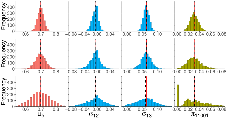
Figure 2: Examples of the sampling distributions of the $\mathrm{MAP}$ estimates for the mean parameter $\mu_{5}$, covariance parameters $\sigma_{12}$, $\sigma_{13}$, and the joint distribution by the estimated model $\pi(x_{P}=(1,1,0,0,1))$. The first, second and third rows correspond to the results of the sample sizes $N=500$, $N=200$ and $N=50$, respectively. The trial size, i.e., the number of times the estimates are computed, is $M=2000$. The red solid lines denote the true values and the black dashed lines denote the mean values of the sampling distributions.

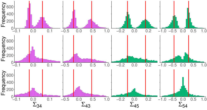
Figure 3: Examples of the sampling distributions of the $\mathrm{MAP}$ estimates for parameters $\Sigma_{ij}$. The first, second and third rows correspond to the results of the sample sizes $N=5000$, $N=500$ and $N=50$, respectively. The trial size is $M=2000$. The red solid lines denote the value of the true parameters. Due to the degrees of freedom of the matrix transposition, there exist two lines corresponding to the true parameters.

Fig. 2 shows the sampling distributions of the $\mathrm{MAP}$ estimates for the mean and covariance parameters and the joint distribution by the estimated model for different sample sizes $N$. The data are generated by the same model as the previous subsection. As in the case of statistics, we observe that each estimate converges to the true values of the parameters asymptotically as the sample size goes to infinity. Although the sampling distribution can be skewed when the sample size is small, it becomes asymptotically normal as the sample size increases. In other words, our $\mathrm{MAP}$ estimator is consistent and asymptotically normal. The standard errors of the sampling distributions decrease as $1/\sqrt{N}$ as the sample size increases. These results suggest that the usual statistical inference on model parameters such as hypothesis testing and confidence interval estimation is available.

Fig. 3 shows the sampling distributions of the $\mathrm{MAP}$ estimates for the parameters $\Sigma_{ij}$ for different sample sizes $N$. Here, we note the degrees of freedom for the model parameters. Since the joint distribution is given by the determinant of the matrix $\Sigma$ as in Eq. (40), the elements of the matrix are not determined uniquely. That is, there exist different parameters that generate the same joint probabilities. In fact, the determinants of the matrix of the form of Eq. (40) are invariant under multiplying an $i$-th row of the matrix $\Sigma$ by a constant $c$ at the same time multiplying the $i$-th column with the same index $i$ by the constant $1/c$. Furthermore, the determinants are invariant under the matrix transposition. These degrees of freedom can also be read from the expression for the Grassmann integral. Hence, without loss of generality, we fix the parameters $\Sigma_{i1}=-1\;\,(i\neq 1)$ using the degrees of freedom for the constant multiplication. That is, the parameters $\Sigma_{1j}\;\,(j\neq 1)$ simply represent the covariances. However, we failed to find a way to fix the degree of freedom for the matrix transposition. Hence, in Fig. 3, we show both of the estimated parameters corresponding to the degrees of freedom for the matrix transposition. Although when the sample size is small the sampling distribution of the estimate $\Sigma_{ij}$ has large dispersion and is unimodal, the estimates converge to one of the true parameters as the sample size goes to infinity.

IV Conclusion

We formulated a probability distribution for multivariate binary variables using the Grassmann number. Performing summation over states by integration of the Grassmann variables, we derived analytical expressions for the partition function, the central moment, and the joint, marginal and conditional distributions. These distributions are expressed by the matrix of the parameters $\Sigma$, which is a matrix analogous to the covariance matrix in the multivariate Gaussian distribution. The proposed method has many similarities to the multivariate Gaussian distribution. For example, a principal submatrix of $\Sigma$ expresses the marginal distribution, the diagonal elements of which express the mean parameters, and the products of the off-diagonal elements express the covariance. The inverse matrix $\Lambda=\Sigma^{-1}$ expresses the conditional distribution; the diagonal element expresses the inverse of the mean and the off-diagonal element can be interpreted as a kind of partial correlation conditioned on all the other variables. The uncorrelatedness of variables for the marginal and conditional distributions is equivalent to unconditional and conditional independence, respectively. Furthermore, the joint probabilities corresponding to all $2^{p}$ possible states for a $p$-dimensional binary variables are expressed as all possible principal minors of the matrix $\Lambda-I$. The property that all joint probabilities must be greater than or equal to zero can be rephrased in the terminology of linear algebra as that the matrix $\Lambda-I$ must be a $P_{0}$-matrix. These properties are in contrast to those of the conventional multivariate Bernoulli distribution, where the joint probabilities of all states are always greater than zero because it is expressed as an exponential function of a polynomial in the dummy variables.

We validated our method numerically. Since we have analytical expressions for the marginal and conditional distributions, we can easily generate random numbers of the correlated binary variables by repeating Bernoulli trials. We investigated the sampling distributions of various statistics and $\mathrm{MAP}$ estimates by using synthetic datasets. We demonstrated that the sampling distributions of various statistics are consistent with the theoretical predictions. We observed that our $\mathrm{MAP}$ estimates are consistent and asymptotically normal.

Since our method has many similarities to the multivariate Gaussian distribution, it has many potential applications, where the covariance structure of random variables is extensively utilized. Examples include the hierarchical and non-hierarchical clustering, such as $k$-means clustering and the mixture distribution model, and anomaly detection like the Hotelling’s $T^{2}$ method. There, a method similar to the multivariate Gaussian distribution will be extended and applied to binary random variables. It is important to demonstrate that the proposed method can describe real data well. Our method in turn will also be useful in studying the behavior of gases or magnets in statistical physics, which have conventionally been analyzed using the Ising model.

Further direction of theoretical research is to develop an estimation procedure for model parameters. In our method, we have to estimate model parameters with which the joint probabilities of all possible states must be positive. The parameter estimation procedure employed in this paper is limited to the case where the number of variables $p$ is small due to computational complexity, since the objective function, i.e., the logarithm of the posterior distribution, has all terms corresponding to the number of all $2^{p}$ possible states. Hence, it is desirable to develop an efficient procedure for parameter estimation that ensures the positivity of all joint probabilities when the number of variables is large, to take advantage of our method that the analytical expressions are given. Another direction is to explore theoretical properties of the sampling distribution of an estimated parameter to make a statistical inference on model parameters such as hypothesis testing and confidence interval estimation. Lastly, we expect our method to be a framework for dealing with qualitative random variables as an alternative to the method of quantification.

References

- Ising (1925) E. Ising, Z. Physik 31, 253–258 (1925).
- Geman and Geman (1984) S. Geman and D. Geman, IEEE Transactions on Pattern Analysis and Machine Intelligence PAMI-6, 721 (1984).
- Ackley et al. (1985) D. H. Ackley, G. E. Hinton, and T. J. Sejnowski, Cognitive Science 9, 147 (1985).
- Banerjee et al. (2008) O. Banerjee, L. El Ghaoui, and A. d’Aspremont, J. Mach. Learn. Res. 9, 485–516 (2008).
- Xue et al. (2012) L. Xue, H. Zou, and T. Cai, Ann. Statist. 40, 1403 (2012).
- Wainwright and Jordan (2008) M. J. Wainwright and M. I. Jordan, Graphical Models, Exponential Families, and Variational Inference (2008).
- Höfling and Tibshirani (2009) H. Höfling and R. Tibshirani, Journal of Machine Learning Research 10, 883 (2009).
- Ravikumar et al. (2010) P. Ravikumar, M. J. Wainwright, and J. D. Lafferty, Ann. Statist. 38, 1287 (2010).
- Manning and Schütze (1999) C. D. Manning and H. Schütze, Foundations of Statistical Natural Language Processing (MIT Press, Cambridge, MA, USA, 1999).
- Woods (1978) J. Woods, IEEE Transactions on Automatic Control 23, 846 (1978).
- Hassner and Sklansky (1980) M. Hassner and J. Sklansky, Computer Graphics and Image Processing 12, 357 (1980).
- RIPLEY (1981) B. D. RIPLEY, Spatial Statistics. (Wiley, New York., 1981).
- Dai et al. (2013) B. Dai, S. Ding, and G. Wahba, Bernoulli 19, 1465 (2013).
- Peskin and Schroeder (1995) M. E. Peskin and D. V. Schroeder, An Introduction to quantum field theory (Addison-Wesley, Reading, USA, 1995).
- Berman and Plemmons (1994) A. Berman and R. J. Plemmons, Nonnegative Matrices in the Mathematical Sciences (Society for Industrial and Applied Mathematics, 1994).