Hall coefficient of semimetals

Abstract

A recently developed formula for the Hall coefficient [A. Auerbach, Phys. Rev. Lett. 121, 66601 (2018)] is applied to nodal line and Weyl semimetals (including graphene), and to spin-orbit split semiconductor bands in two and three dimensions. The calculation reduces to a ratio of two equilibrium susceptibilities, where corrections are negligible at weak disorder. Deviations from Drude’s inverse carrier density are associated with band degeneracies, Fermi surface topology, and interband currents. Experiments which can measure these deviations are proposed.

Semimetals are characterized by proximity of the Fermi energy to band degeneracies. Vigorous research has been recently invested in semimetals on surfaces of topological insulators TI1 ; TI2 , Dirac and Weyl semimetals Weyl1 ; Weyl2 ; Weyl3 ; NodalSM1 ; NodalSM2 ; NodalSM3 , and on semimetal platforms for Majorana states applications Majorana .

This paper focuses on the Hall coefficient of semimetals, which has been traditionally used to measure the charge carrier density $n$ using Drude’s relation $R_{\rm H}\propto n^{-1}$. In semimetals, Drude’s relation may break down due to multiband effects, and Fermi surface topology. For example, corrections to Drude’s relation was found by Liu et al.Culcer for spin-orbit split semiconductor bands. Multiband conductivity calculations involve coupled Boltzmann equations with interband collision integrals which are quite challenging Bulbul ; Assa-Allen .

We can avoid coupled Boltzmann equations by applying the Hall coefficient formula PRL ; EMT to multiband Hamiltonians. The dissipative scattering rates drop out, and $R_{\rm H}$ is primarily determined by the non-dissipative Lorentz force captured by the current-magnetization-current (CMC) susceptibility $\chi^{\vphantom{\dagger}}_{\scriptscriptstyle\textsf{CMC}}$, and the conductivity sum rule (CSR) $\chi^{\vphantom{\dagger}}_{\scriptscriptstyle\textsf{CSR}}$. Both coefficients are non dissipative: the CMC describes the effect of the Lorentz force on the currents, and the CSR governs their reactive response.

Crucial to our approach is the estimation of the formula’s correction term ${\cal R}^{\rm corr}$, which is determined by higher moments of the dynamical conductivity. This paper shows that in the “good quasiparticles” (Boltzmann) regime, ${\cal R}^{\rm corr}$ can be neglected for disorder strength less than the Fermi energy.

Our key results are: (i) For Weyl point semimetals in two and three dimensions, (including graphene) the intraband $R_{\rm H}^{\scriptscriptstyle\textsf{INTRA}}(n)$ exhibits a Drude-like divergence, which is cut off by interband scattering at low densities. (ii) The nodal line semimetal (see Fig. 1) exhibits a constant (rather than diverging) Hall coefficient, with a sign change at the nodal energy. (iii) Previous results Culcer of spin-orbit split bands are extended into the interband transport regime, and to three dimensions. (iv) ${{\cal R}^{\rm corr}}$ is shown to be relatively suppressed by the disorder potential fluctuations divided by the Fermi energy squared. The paper ends with a summary and proposals for experiments.

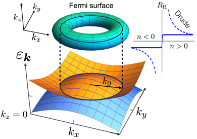
Figure 1: Nodal line semimetal. The nodal line is marked by black circle of radius $k_{0}$. The three dimensional toroidal Fermi surface (top) is depicted. At the upper right corner, the qualitative behavior of the Hall coefficient (solid line) is compared to Drude relation, for density $n$ as measured from the nodal circle filling.

The Hall coefficient formula , as derived directly from the Kubo formulas  PRL ; EMT for any Hamiltonian ${\cal H}$ and spectrum $\{E_{n},|n\rangle\}$,

$$R_{\rm H}\equiv\lim_{B\to 0}\bigg{(}\sigma_{xx}^{-2}\,{\partial\sigma_{xy}\over\partial B}\bigg{)}={\chi^{\vphantom{\dagger}}_{\scriptscriptstyle\textsf{CMC}}\over\chi^{2}_{\scriptscriptstyle\textsf{CSR}}}+{\cal R}^{\rm corr}.$$ (1)

$\sigma_{\alpha\beta}$ is the conductivity tensor (assuming C4 symmetry) and $B$ is the magnetic field in the $z$-direction. $\chi^{\vphantom{\dagger}}_{\scriptscriptstyle\textsf{CMC}}={\rm Im}\big{(}j^{y},[M,j^{x}]\big{)}-{\rm Im}\big{(}j^{x},[M,j^{y}]\big{)}$ and $\chi^{\vphantom{\dagger}}_{\scriptscriptstyle\textsf{CSR}}=\big{(}j^{x},j^{x}\big{)}$, where $j^{\alpha}$ is the uniform current in the $\alpha$ direction, and $M=\partial{\cal H}/\partial B$ is the diamagnetization operator. The inner products are defined by equilibrium susceptibilities, SM ,

$$(j^{\alpha},A)={1\over Z}\sum_{nm}{e^{-\beta E_{n}}-e^{\-\beta E_{m}}\over E_{m}-E_{n}}\langle n|j^{\alpha}|m\rangle\langle m|A|n\rangle\quad,$$ (2)

where $Z={\rm Tr}e^{-\beta{\cal H}}$ and $\beta$ is the inverse temperature.

The correction term ${\cal R}^{\rm corr}$ is given by

$${\cal R}^{\rm corr} ={1\over\chi^{\vphantom{\dagger}}_{\scriptscriptstyle\textsf{CSR}}}\sum_{i,j=0}^{\infty}(1-\delta^{\vphantom{\dagger}}_{i,0}\,\delta^{\vphantom{\dagger}}_{j,0}){\cal M}^{\prime\prime}_{2i,2j}$$ (3)

$$\qquad\times\prod_{i^{\prime}=0}^{i}\left(-{\Delta_{2i^{\prime}-1}\over\Delta_{2i^{\prime}~{}~{}}}\right)\prod_{j^{\prime}=0}^{j}\left(-{\Delta_{2j^{\prime}-1}\over\Delta_{2j^{\prime}~{}~{}}}\right)\quad.$$

${\cal M}^{\prime\prime}_{2i,2j}$ are cross-susceptibilities, defined by the matrix elements of the magnetization commutator $[M,\bullet]$ between two currents’ Krylov bases. The Krylov bases are generated by orthonormalizing the sets of operators $[{\cal H},[\>\cdots,[{\cal H},j^{\alpha}]]]$. $\Delta_{i^{\prime}}$ are the conductivity recurrents LA , which can be obtained from the conductivity moments, defined by $\mu_{2i}=\langle\big{[}j^{x},[{\cal H},[\>\cdots,[{\cal H},j^{x}]]]\big{]}\rangle$, where ${\cal H}$ appears $2i-1$ times. Instructions for calculating ${\cal M}^{\prime\prime}_{2i,2j}$ and $\Delta_{i^{\prime}}$ are reviewed in SM . Physically, ${\cal R}^{\rm corr}$ incorporates the higher order effects of current non-conservation. In several examples, its relative magnitude can be suppressed by using a renormalized Hamiltonian EMT . Later, we estimate ${\cal R}^{\rm corr}$ and show that it can be neglected in regimes of weak disorder which concern this paper.

We consider a general two-band Hamiltonian,

$${\cal H}_{0}\equiv\sum_{\boldsymbol{k}}\sum_{l,l^{\prime}=1}^{2}c^{\dagger}_{l{\boldsymbol{k}}}\,h^{\vphantom{\dagger}}_{ll^{\prime}}({\boldsymbol{k}})\,c^{\vphantom{\dagger}}_{l^{\prime}{\boldsymbol{k}}}\quad.$$ (4)

where $c^{\dagger}_{l{\boldsymbol{k}}}$ creates a Bloch electron on band $l$ and wavevector ${\boldsymbol{k}}$. A random potential with fluctuation $V^{2}_{\rm dis}$ introduces a transport scattering rate $\hbar/\tau_{\rm tr}\sim V_{\rm dis}^{2}/|\varepsilon_{\rm F}|$, where $\varepsilon_{\rm F}$ is the Fermi energy measured from the nearest particle-hole symmetric energy or band extremum.

Within the “good quasiparticles” regime, $\hbar/\tau_{\rm tr}\ll\varepsilon_{\rm F}^{\vphantom{\dagger}}$, the ratio of the disorder strength to interband gap at the Fermi energy $\Delta\varepsilon$, defines two distinct transport regimes. Importantly, for evaluation of Eq. (1), we have the freedom to choose the (renormalized) effective Hamiltonian which best describes the low energy correlations. Our choice determines the values of $\chi^{\vphantom{\dagger}}_{\scriptscriptstyle\textsf{CMC}},\chi^{\vphantom{\dagger}}_{\scriptscriptstyle\textsf{CSR}}$ and ${{\cal R}^{\rm corr}}$. It is the latter we wish to minimize.

(i) Intraband regime applies for $V_{\rm dis}^{2}\ll(\Delta\varepsilon)^{2}$, where interband scattering is suppressed, and transport is dominated by band-diagonal current and magnetization operators:

$${j^{\alpha}_{\scriptscriptstyle\textsf{INTRA}}} = e\sum_{i,{\boldsymbol{k}}}c^{\dagger}_{i{\boldsymbol{k}}}\,v^{\alpha}_{i}({\boldsymbol{k}})\,c^{\vphantom{\dagger}}_{i{\boldsymbol{k}}}~{},~{}\alpha=x,y~{},\quad i=1,2,$$

$${M_{\scriptscriptstyle\textsf{INTRA}}} = {ie\over 2c}\sum_{i,{\boldsymbol{k}}}c^{\dagger}_{i{\boldsymbol{k}}}\,\bigg{(}\!v^{y}_{i}({\boldsymbol{k}}){\partial\over\partial k_{x}}-v^{x}_{i}({\boldsymbol{k}}){\partial\over\partial k_{y}}\bigg{)}\,c^{\vphantom{\dagger}}_{i{\boldsymbol{k}}}$$ (5)

with $v^{\alpha}_{i}({\boldsymbol{k}})=\partial\varepsilon^{\vphantom{\dagger}}_{i}({\boldsymbol{k}})/\partial k_{\alpha}$, where $\varepsilon^{\vphantom{\dagger}}_{i}({\boldsymbol{k}})$ $(i\!=\!1,2)$ are the eigenvalues of $h_{ll^{\prime}}({\boldsymbol{k}})$. The susceptibilities in this regime are SM ,

$$\begin{split}\chi_{\scriptscriptstyle\textsf{CMC}}^{\scriptscriptstyle\textsf{INTRA}}&={e^{3}\over c}\sum_{i=1}^{2}\int\!{d^{d}k\over(2\pi)^{d}}\,F^{\vphantom{\dagger}}_{i}({\boldsymbol{k}})\,\bigg{(}\!\!-{\partial f\over\partial\varepsilon}\bigg{)}^{\vphantom{\dagger}}_{\!\varepsilon=\varepsilon^{\vphantom{\dagger}}_{i}({\boldsymbol{k}})}\\ F^{\vphantom{\dagger}}_{i}({\boldsymbol{k}})&=\big{[}v^{y}_{i}({\boldsymbol{k}})\big{]}^{\!2}\,{\partial v^{x}_{i}({\boldsymbol{k}})\over\partial k_{x}}-v^{x}_{i}({\boldsymbol{k}})\,v^{y}_{i}({\boldsymbol{k}})\,{\partial v^{y}_{i}({\boldsymbol{k}})\over\partial k_{x}}\\ \chi_{\scriptscriptstyle\textsf{CSR}}^{\scriptscriptstyle\textsf{INTRA}}&=e^{2}\sum_{i=1}^{2}\int\!{d^{d}k\over(2\pi)^{d}}\,\big{(}v^{x}_{i}({\boldsymbol{k}})\big{)}^{\!2}\bigg{(}\!\!-{\partial f\over\partial\varepsilon}\bigg{)}^{\vphantom{\dagger}}_{\!\varepsilon=\varepsilon^{\vphantom{\dagger}}_{i}({\boldsymbol{k}})}\quad.\end{split}$$ (6)

$f_{i}$ is the Fermi-Dirac distribution of band $\varepsilon^{\vphantom{\dagger}}_{i}({\boldsymbol{k}})$ at temperature $T$ and chemical potential $\varepsilon_{\rm F}$. For any spherically symmetric band, $\varepsilon({\boldsymbol{k}})=\varepsilon(k)$, Drude’s relation holds, i.e. $R_{\rm H}=\chi^{\vphantom{\dagger}}_{\scriptscriptstyle\textsf{CMC}}/\chi_{\scriptscriptstyle\textsf{CSR}}^{2}=1/(nec)$ Comm-elliptical . For more general band structures, Eqs. (6) recovers the venerable Boltzmann equation result in the “isotropic scattering limit” Ziman ; Comm-ISL .

(ii) Interband regime applies within the range $(\Delta\varepsilon)^{2}\leq V_{\rm dis}^{2}\ll\varepsilon_{\rm F}^{2}$, where disorder is strong enough to mix the two bands (but still weak enough to neglect ${{\cal R}^{\rm corr}}$, see later discussion). Interband currents now contribute to the longitudinal conductivity and to $\chi^{\vphantom{\dagger}}_{\scriptscriptstyle\textsf{CSR}}$ Bulbul ; Mohit . In this regime, the susceptibilities must involve full two-band operators represented by $2\times 2$ matrices,

$$\begin{split}j^{\alpha}_{ll^{\prime}}({\boldsymbol{k}})&\equiv e\,{\partial h^{\vphantom{\dagger}}_{ll^{\prime}}({\boldsymbol{k}})\over\partial k_{\alpha}}\\ M_{ll^{\prime}}({\boldsymbol{k}})&\equiv{ie\over 2c}\bigg{(}j_{ll^{\prime}}^{y}({\boldsymbol{k}})\,{\partial\over\partial k_{x}}-j_{ll^{\prime}}^{x}({\boldsymbol{k}})\,{\partial\over\partial k_{y}}\bigg{)}\quad,\end{split}$$ (7)

which yield the interband susceptibilities which can be conveniently expressed by SM ,

$$\chi_{\scriptscriptstyle\textsf{CMC}}^{\scriptscriptstyle\textsf{INTER}} =\!\int\!{d^{d}k\over(2\pi)^{d}}\sum_{i=1}^{2}f\big{(}\varepsilon^{\vphantom{\dagger}}_{i}({\boldsymbol{k}})\big{)}\,F^{\scriptscriptstyle\textsf{INTER}}_{i}({\boldsymbol{k}})$$

$$F^{\scriptscriptstyle\textsf{INTER}}_{i}({\boldsymbol{k}}) =e\bigg{[}U^{\dagger}_{\boldsymbol{k}}\,\bigg{(}{\partial\over\partial k_{y}}\,\big{[}M,j^{x}\big{]}-{\partial\over\partial k_{x}}\big{[}M,j^{y}\big{]}\bigg{)}U_{\boldsymbol{k}}\bigg{]}^{\vphantom{\dagger}}_{\!ii}$$

$$\chi_{\scriptscriptstyle\textsf{CSR}}^{\scriptscriptstyle\textsf{INTER}} =e\!\int\!{d^{d}k\over(2\pi)^{d}}\!\sum_{i=1}^{2}f\big{(}\varepsilon^{\vphantom{\dagger}}_{i}({\boldsymbol{k}})\big{)}\,\bigg{[}U_{\boldsymbol{k}}^{\dagger}\,{\partial j^{x}({\boldsymbol{k}})\over\partial k_{x}}\,U_{\boldsymbol{k}}\bigg{]}_{\!ii}$$ (8)

The unitary matrix $U_{\boldsymbol{k}}$ diagonalizes $h({\boldsymbol{k}})$. We note that the operator $\partial\big{[}M,j^{\alpha}\big{]}/\partial k^{\beta}$ includes a derivative $\partial/\partial k_{\alpha}$ acting to the right on $U_{\boldsymbol{k}}$. This derivative captures the effect of SU(2) rotation of Bloch states inside the Fermi volume.

We now apply Eqs. (6) and (Hall coefficient of semimetals) to calculate the Hall coefficients of the following models.

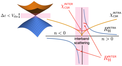
Figure 2: The two dimensional Weyl cone, whose bands are depicted in the upper left. The intraband Hall coefficient (online, blue) and conductivity sum rule (online, orange) are plotted versus the density of carriers $n$ as measured from the nodal filling. Pink (online) regions mark the low density interband dominated transport regime, where the interband gap is lower than the disorder potential $V_{\rm dis}$. In this regime, the conductivity sum rule $\chi^{\scriptscriptstyle\textsf{INTER}}_{\scriptscriptstyle\textsf{CSR}}$ does not vanish at the nodal density, and the Drude-like divergence of the Hall coefficient is cut off (see text).

Weyl semimetals.—When the product of time reversal and inversion is not a symmetry of a system, the band structure may exhibit Weyl points, where two bands intersect at the Fermi level. Expansion of the semimetal band structure near a linear point degeneracy results in the $d$-dimensional 2-band Weyl Hamiltonian Comm-WeylSM

$$H^{\vphantom{\dagger}}_{0}=v^{\vphantom{\dagger}}_{0}\,{\boldsymbol{k}}\cdot{\boldsymbol{\sigma}}$$ (9)

which yields the conical dispersion $\varepsilon^{\vphantom{\dagger}}_{\pm}({\boldsymbol{k}})=\pm v_{0}\,|{\boldsymbol{k}}|$, see Fig. 2. For $d=2$, this could describe surface states of a three dimensional topological insulator TI1 , or a single Dirac cone in graphene Graphene-CN . For $d=3$, this could describe one Weyl cone in a Weyl semimetal.

The density (per cone) is $n=\textsf{sgn}(n)\,k_{\rm F}^{d}/2d\pi^{d-1}$, where $k_{\rm F}$ is the Fermi wavevector. In the intraband transport regime,

$$\begin{split}\chi_{\scriptscriptstyle\textsf{CMC}}^{\scriptscriptstyle\textsf{INTRA}}&={e^{4}v_{0}^{2}\over c}{k_{\rm F}^{d-2}\over 2d\pi^{d-1}}\,\textsf{sgn}(n)\propto\textsf{sgn}(n)\,|n|^{(d-2)/d}\\ \chi_{\scriptscriptstyle\textsf{CSR}}^{\scriptscriptstyle\textsf{INTRA}}&={v_{0}\over 2d\pi^{d-1}}k_{F}^{d-1}\propto|n|^{(d-1)/d}\quad,\end{split}$$ (10)

which recovers the Drude relation $R^{\scriptscriptstyle\textsf{INTRA}}_{H}=1/nec$.

For the interband regime SM we find that,

$$\chi^{\scriptscriptstyle\textsf{INTER}}_{\scriptscriptstyle\textsf{CMC}}(n)=\chi_{\scriptscriptstyle\textsf{CMC}}^{\scriptscriptstyle\textsf{INTRA}}(n)\quad,\quad\chi^{\scriptscriptstyle\textsf{INTER}}_{\rm CSR}(n)\propto n^{0}.$$ (11)

At low densities, the interband regime takes over when $\Delta\varepsilon<V^{\vphantom{\dagger}}_{\rm dis}$, as depicted by pink (online) shaded areas in Fig. 2. Since the sum rule in Eq. (11) does not vanish at the Weyl point the Drude-like divergence of the Hall coefficient is cut off at the Weyl point.

Unfortunately, a quantitative calculation of $R^{\scriptscriptstyle\textsf{INTER}}_{\rm H}$ in this regime is not available, since the Fermi energy is half the interband gap. This violates the “good quasiparticles” condition, and ${{\cal R}^{\rm corr}}$ cannot be neglected (as explained later). Nevertheless, since $\chi^{\scriptscriptstyle\textsf{INTER}}_{\scriptscriptstyle\textsf{CSR}}>0$, the saturation of $R_{\rm H}^{{\scriptscriptstyle\textsf{INTER}}}<\infty$ at the Weyl point still holds.

Nodal-line semimetal.—It is also possible for two bands to touch along a curve, as is the case in a nodal line semimetal NodalSM1 ; NodalSM4 . Such a state of affairs has reportedly been observed in the compound ZrSiSe NLS_basov as well as in optical lattices with ultracold fermions NLS_optical .

We consider a nodal circle of radius $k_{0}$ in the $k_{z}$=0 plane, as depicted in Fig. 1. The dispersions near the nodal line are expanded for low values of $\delta k_{\perp}=\sqrt{k_{x}^{2}+k_{y}^{2}}-k_{0}$ and $k_{z}$,

$$\varepsilon_{{\boldsymbol{k}}\pm}\simeq\pm v_{0}\sqrt{\alpha^{2}\big{(}\delta k^{\vphantom{\dagger}}_{\perp}\big{)}^{\!2}+k_{z}^{2}}$$ (12)

where $\alpha$ is a dimensionless anisotropy parameter. Here we limit the calculation to the intraband regime at zero temperature, where $n={k_{0}\varepsilon_{\rm F}^{2}/4\pi\alpha v_{0}^{2}}$. By Eq. (6), the susceptibilities are

$$\chi_{\scriptscriptstyle\textsf{CMC}}^{\scriptscriptstyle\textsf{INTRA}}={3e^{3}v^{2}_{0}\alpha^{2}n\over 4k_{0}^{2}c}\quad,\quad\chi_{\scriptscriptstyle\textsf{CSR}}^{\scriptscriptstyle\textsf{INTRA}}=e^{2}v_{0}\left({\alpha^{3}k_{0}n\over 16\pi}\right)^{\!\!1/2},$$ (13)

which yields an unusual density dependence of the Hall coefficient,

$$R^{\scriptscriptstyle\textsf{INTRA}}_{\rm H}={12\pi\over\alpha k_{0}^{3}ec}~{}\textsf{sgn}(n)$$ (14)

The nodal line semimetal exhibits a density independent Hall coefficient with an abrupt sign reversal, at zero temperature and disorder. The suppression of $\chi_{\scriptscriptstyle\textsf{CMC}}^{\scriptscriptstyle\textsf{INTRA}}$ at large radii can be intuitively attributed to the near cancellation of the inner (hole-like) and outer (electron-like) sides of the toroidal Fermi surface.

The density dependences of Weyl and nodal line semimetals are summarized in Table 1.

Model	$\chi_{\scriptscriptstyle\textsf{CSR}}^{\scriptscriptstyle\textsf{INTRA}}$	$R_{\rm H}^{\scriptscriptstyle\textsf{INTRA}}$	$\chi_{\scriptscriptstyle\textsf{CSR}}^{\scriptscriptstyle\textsf{INTER}}$	$R_{\rm H}^{\scriptscriptstyle\textsf{INTER}}$
2d Weyl	$|n|^{1/2}$	$1/n$	const	$\leq{\rm const}$
3d Weyl	$|n|^{2/3}$	$1/n$	const	$\leq|n|^{1/3}$
nodal line sm	$|n|^{1/2}$	$\textsf{sgn}(n)$

Table 1: Nodal line semimetal and Weyl semimetals in 2 and 3 dimensions. The density dependence of the conductivity sum rules and Hall coefficients are given for the intraband and interband transport regimes.

Semiconductor bands.—with an inversion-asymmetric zinc blende structure, e.g. GaAs and CdTe, are subjected to spin orbit interactions described by the Kane and Luttinger models KaneModel ; Luttinger ; Winkler . They share with semimetals the small interband gaps near the Fermi energy. We study two models: (i) The (heavy) hole bands in a two dimensional quantum well (2dH) Culcer :

$$h^{\textsf{2dH}}({\boldsymbol{k}})={k^{2}\over 2m}\mathbb{I}\ \pm\ \beta\left[k_{y}(k_{y}^{2}-3k_{x}^{2})\,\sigma^{x}+k_{x}(k_{x}^{2}-3k_{y}^{2})\,\sigma^{y}\right]$$ (15)

where the Rashba parameter $\beta$ depends on the perpendicular electric field Culcer . The bands $\varepsilon^{\textsf{2dH}}_{{\boldsymbol{k}}\pm}={k^{2}/2m}\pm\beta k^{3}$ are rotationally symmetric, and split by $\beta$.

(ii) The conduction band in a cubic crystal, with spin orbit interaction splitting expanded up to third order in $k$ Winkler ,

$$h^{\textsf{3dC}}({\boldsymbol{k}}) ={k^{2}\over 2m}\mathbb{I}\pm\beta\,{\boldsymbol{h}}({\boldsymbol{k}})\cdot{\boldsymbol{\sigma}}$$ (16)

$${\boldsymbol{h}}({\boldsymbol{k}}) =\big{(}k_{y}^{2}-k_{z}^{2}\big{)}k_{x}{\hat{\boldsymbol{x}}}+\big{(}k_{z}^{2}-k_{x}^{2}\big{)}k_{y}{\hat{\boldsymbol{y}}}+\big{(}k_{x}^{2}-k_{y}^{2}\big{)}k_{z}{\hat{\boldsymbol{z}}}$$

the dispersions $\varepsilon^{\textsf{3dC}}_{{\boldsymbol{k}}\pm}={k^{2}/2m}\pm\beta|{\boldsymbol{h}}_{\boldsymbol{k}}|$, have cubic symmetry.

We find that for both models, Eq. (15) and 16), the susceptibilities and Hall coefficients are corrected by terms of order order $\beta^{2}$:

$$\chi_{\scriptscriptstyle\textsf{CSR}}={e^{2}\over m}\left(n+\beta^{2}\Delta\chi_{\scriptscriptstyle\textsf{CSR}}\right),\quad R_{\rm H}={1+\beta^{2}{\cal K}(n)\over nec}\quad,$$ (17)

The results for the corrections of both Eq. (15) and (16) are listed in Table 2. The density dependence and sign of the intraband corrections for the heavy holes model (15) are consistent with Ref.  Culcer . Our new results for the interband regime SM show that while $\chi^{\scriptscriptstyle\textsf{INTER}}_{\scriptscriptstyle\textsf{CMC}}=\chi^{\scriptscriptstyle\textsf{INTRA}}_{\scriptscriptstyle\textsf{CMC}}$, the sum rule is different, since it acquires no order $\beta^{2}$ corrections, i.e. $\chi^{\scriptscriptstyle\textsf{INTER}}_{\scriptscriptstyle\textsf{CSR}}={e^{2}n\over m}$. As a result, we obtain that ${\cal K}^{\scriptscriptstyle\textsf{INTER}}=-{\cal K}^{\scriptscriptstyle\textsf{INTRA}}$, that is to say, the spin-orbit correction to the Drude Hall coefficient reverses sign as disorder increases between the intraband and interband scattering regimes.

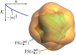
Figure 3: Spin-orbit split Fermi surfaces (FS) of conduction electrons described by the Hamiltonian Eq. (16). Top left: Density dependence of the non-Drude correction ${\cal K}$, Eq. (17).

For $h^{\textsf{3dC}}({\boldsymbol{k}})$, the spin-orbit correction $\Delta\chi^{\textsf{3dC}}_{\scriptscriptstyle\textsf{CSR}}$ is of order $-n^{5/3}$ due to the $k^{3}$ scaling of ${\boldsymbol{h}}({\boldsymbol{k}})$. The interband susceptibility $\chi^{\scriptscriptstyle\textsf{INTER}}_{\scriptscriptstyle\textsf{CMC}}$ is not equal in magnitude to $\chi^{\scriptscriptstyle\textsf{INTRA}}_{\scriptscriptstyle\textsf{CMC}}$, which appears to be due to non-spherical symmetry of the bandstructure, as shown in Fig. 3.

Model	$\Delta\chi_{\scriptscriptstyle\textsf{CSR}}^{\scriptscriptstyle\textsf{INTRA}}/m^{2}$	${\cal K}^{\scriptscriptstyle\textsf{INTRA}}/m^{2}$	${\cal K}^{\scriptscriptstyle\textsf{INTER}}/m^{2}$
2dH	$-18\pi n^{2}$	$18\pi n$	$-18\pi n$
3dC	$-8.0(1)\,n^{5/3}$	$-17.5(1)\,n^{2/3}$	$-23.0(1)\,n^{2/3}$

Table 2: Spin-orbit corrections to the sum rule and Hall coefficient factor for the two dimensional hole bands Eq. (15), and three dimensional conduction bands, Eq. (16). Results for the intraband and interband transport regimes are displayed. The conductivity sum rule receives no order $\beta^{2}$ correction in the interband regime.

Estimation of the correction ${\cal R}^{\rm corr}$.—We now prove that ${\cal R}^{\rm corr}$, of Eq. (3), vanishes as (at least) two powers of the disorder potential over the Fermi energy. Explicit instructions to calculate the moments, recurrents, Krylov bases and magnetization matrix elements EMT are reviewed in SM . Let us first consider the intraband scattering regime where $V_{\rm dis}\ll\Delta\varepsilon\ll\varepsilon_{\rm F}$:

The intraband currents commute with the clean Hamiltonian $[{\cal H}_{0},{j^{\alpha}_{\scriptscriptstyle\textsf{INTRA}}}^{x}]=0$. Hence the high order Krylov operators are produced by commuting the current with at least one power of the disorder potential. The magnetization matrix elements between normalized Krylov bases should therefore scale as,

$$(1-\delta_{i,0}\delta_{j,0})|{\cal M}^{\prime\prime}_{2i,2j}|\propto{\chi^{\vphantom{\dagger}}_{\scriptscriptstyle\textsf{CMC}}\over\chi^{\vphantom{\dagger}}_{\scriptscriptstyle\textsf{CSR}}}\left({V_{\rm dis}\over\varepsilon_{\rm F}}+{\cal O}\left({V_{\rm dis}\over\varepsilon_{\rm F}}\right)^{2}\right)$$ (18)

For similar reasons, the first two conductivity moments scale as,

$$\begin{split}\mu_{2}&\propto\chi^{\vphantom{\dagger}}_{\scriptscriptstyle\textsf{CSR}}\,V^{2}_{\rm dis}\\ \mu_{4}&\propto\chi^{\vphantom{\dagger}}_{\scriptscriptstyle\textsf{CSR}}\,\left(\varepsilon_{\rm F}^{2}V^{2}_{\rm dis}+{\cal O}(V^{4}_{\rm dis})\right),\end{split}$$ (19)

Transforming moments to recurrents (see SM ) yields the ratio,

$${\Delta_{1}\over\Delta_{2}}=\left({\mu^{2}_{2}\over\chi^{\vphantom{\dagger}}_{\scriptscriptstyle\textsf{CSR}}\,\mu^{\vphantom{\dagger}}_{4}-\mu^{2}_{2}}\right)^{1\over 2}\propto{V_{\rm dis}\over\varepsilon_{\rm F}}.$$ (20)

Combining (18) and (20) in (3), we obtain an overall multiplicative factor,

$$|{\cal R}^{\rm corr}|\propto{|\chi^{\vphantom{\dagger}}_{\scriptscriptstyle\textsf{CMC}}|\over\chi^{2}_{\scriptscriptstyle\textsf{CSR}}}\left({V_{\rm dis}^{2}\over\varepsilon_{\rm F}^{2}}\right).$$ (21)

In the metallic phase, $R_{\rm H},\chi^{\vphantom{\dagger}}_{\scriptscriptstyle\textsf{CMC}}/(\chi^{\vphantom{\dagger}}_{\scriptscriptstyle\textsf{CSR}})^{2}<\infty$, and hence the infinite sum in ${\cal R}^{\rm corr}$ must converge. Therefore the coefficient of proportionality in (21) must be finite.

For the interband regime, we use Eqs. (4,7)) to obtain $\mu_{2}=||~{}[{\cal H},j^{x}]~{}||^{2}\propto\big{(}V^{2}_{\rm dis}+(\Delta\varepsilon)^{2}\big{)}\chi^{\vphantom{\dagger}}_{\scriptscriptstyle\textsf{CSR}}$. We also assume $(\Delta\varepsilon)^{2}\leq V^{2}_{\rm dis}$. Thus, we can appeal again to Eqs. (18,20) by simply replacing $V^{2}_{\rm dis}\to V^{2}_{\rm dis}+(\Delta\varepsilon)^{2}\leq 2V^{2}_{\rm dis}$. This recovers the same proportionality if Eq. (21) as applicable also to the interband regime, where we use $\chi_{\scriptscriptstyle\textsf{CMC}}^{\scriptscriptstyle\textsf{INTER}}/(\chi_{\scriptscriptstyle\textsf{CSR}}^{\scriptscriptstyle\textsf{INTER}})^{2}$ to compute the Hall coefficient Comm-inter-intra . Thus ${\cal R}^{\rm corr}$ can be neglected relative to ratio of corresponding susceptibilities as long as ${V_{\rm dis}^{2}\ll\varepsilon_{\rm F}^{2}}$ in both intraband and interband regimes.

Summary.—Eq. (1) provides insight into deviations from Drude’s relation in semimetals. Our calculations demonstrate the effects of non-spherical and multiple Fermi surfaces, and interband scattering. These effects should be considered when comparing the “Hall number” ($R_{\rm H}^{-1}$) to the Fermi volume, as determined by e.g. angular resolved photoemmision TI2 , and magneto-transport oscillations SdH ; FS-MacKenzie . For time reversal invariant Weyl semimetals, topologically protected surface states have been shown Piet to contribute substantially to the longitudinal conductivity in small samples. Future investigations of the finite size corrections to the Hall coefficient due to surface Fermi arcs states would be interesting. For graphene, we propose to split the Dirac cones by an in plane magnetic field. The Hall coefficient should vanish between gate voltages $V_{\rm gate}=\pm g\mu_{B}B/e$, which may enable measurements of the compressibility at low densities.

Acknowledgement – We acknowledge support from the US-Israel Binational Science Foundation Grant No. 2016168 and the Israel Science Foundation Grant No. 2021367. This research was also supported in part by the ICTS/topmatter2019/12 Program and the program at KITP Santa Barbara, funded by the National Science Foundation under Grant No. NSF PHY-1748958.

I Current cross susceptibilities

Here we derive the expressions leading to Eqs. (6) and (8) in the main text. The general expression of susceptibility between two second quantized operators ${\hat{j}}^{\alpha}$ and ${\hat{A}}$ is [14],

$$({\hat{j}}^{\alpha},{\hat{A}})={1\over Z}\sum_{nm}{e^{-\beta E_{n}}-e^{\-\beta E_{m}}\over E_{m}-E_{n}}\langle n|{\hat{j}}^{\alpha}|m\rangle\langle m|{\hat{A}}|n\rangle,$$ (22)

where $Z={\rm Tr}e^{-\beta{\cal H}}$, $\beta$ is the inverse temperature, and ${\cal H}$ is the full Hamiltonian with spectrum $\{E_{n},|n\rangle\}$. This current susceptibility can be written as an expectation value using the polarization operator

$$({\hat{j}}^{\alpha},{\hat{A}})={1\over Z}\sum_{n}e^{-\beta E_{n}}{\rm Im}\langle n|\left[{\hat{P}}^{\alpha},{\hat{A}}\right]|n\rangle\equiv{\rm Im}\langle\left[{\hat{P}}^{\alpha},{\hat{A}}\right]\rangle,$$ (23)

where ${\hat{P}}^{\alpha}$ is defined by Ehrenfest relation,

$$\left[{\cal H},{\hat{P}}^{\alpha}\right]=i{\hat{j}}^{\alpha}$$ (24)

For band electrons, translationally invariant single particle operators are represented by the bilinear forms,

$${\hat{A}}=\sum_{{\boldsymbol{k}},ll^{\prime}}c^{\dagger}_{{\boldsymbol{k}},l}A_{{\boldsymbol{k}}ll^{\prime}}c_{{\boldsymbol{k}},l^{\prime}},\quad{\hat{j}}=\sum_{{\boldsymbol{k}},ll^{\prime}}c^{\dagger}_{{\boldsymbol{k}},l}j^{\alpha}_{{\boldsymbol{k}},ll^{\prime}}c_{{\boldsymbol{k}},l^{\prime}},$$

$${\cal H}_{0}=\sum_{{\boldsymbol{k}},ll^{\prime}}c^{\dagger}_{{\boldsymbol{k}},l}h_{{\boldsymbol{k}},ll^{\prime}}c_{{\boldsymbol{k}},l^{\prime}},\quad{\hat{P}}^{\alpha}=i\sum_{{\boldsymbol{k}},l}c^{\dagger}_{{\boldsymbol{k}},l}\partial_{k_{\alpha}}c_{{\boldsymbol{k}},l},$$ (25)

where $l,l^{\prime}$ are band indices. The susceptibilities are given by the integrals,

$$({\hat{j}}^{\alpha},{\hat{A}})=\lim_{{\bf q}\to 0}\sum_{ij}{f(\varepsilon_{{\boldsymbol{k}}i})-f(\varepsilon_{{\boldsymbol{k}}+{\bf q}j})\over\varepsilon_{{\boldsymbol{k}}+{\bf q}j}-\varepsilon_{{\boldsymbol{k}}i}}~{}j_{{\boldsymbol{k}}i,{\boldsymbol{k}}+{\bf q}j}^{\alpha}~{}A_{{\boldsymbol{k}}+{\bf q}j,{\boldsymbol{k}}i}~{}.$$ (26)

The intraband currents are diagonal in the eigenstates with dispersion $\varepsilon^{\vphantom{\dagger}}_{i}({\boldsymbol{k}})=(U^{\dagger}_{\boldsymbol{k}}h_{\boldsymbol{k}}U_{\boldsymbol{k}})_{ii}$. Thus, in Eq. (26) only terms with $i=j$ survive, and ${f(\varepsilon_{{\boldsymbol{k}}+{\bf q}i})-f(\varepsilon_{{\boldsymbol{k}}i})\over\varepsilon_{{\boldsymbol{k}}+{\bf q}i}-\varepsilon_{{\boldsymbol{k}}i}}\to\partial_{\varepsilon}f(\varepsilon^{\vphantom{\dagger}}_{i}({\boldsymbol{k}}))$ leading to Eqs. (6) in the main text. For the full interband currents, the susceptibilities are more conveniently expressed using Eq. (23):

$$({\hat{j}}^{\alpha},{\hat{A}})=\sum_{{\boldsymbol{k}},i}f(\varepsilon^{\vphantom{\dagger}}_{i}({\boldsymbol{k}}))\left(U_{\boldsymbol{k}}^{\dagger}\left(\partial_{k_{\alpha}}A_{{\boldsymbol{k}}}\right)U_{{\boldsymbol{k}}}\right)_{ii},$$ (27)

which yield Eqs. (8) in the main text.

II Weyl semimetals

A general Weyl Hamiltonian is

$${\cal H}=v_{0}\left(\sum_{i=1}^{d}a_{i}k_{i}\sigma^{i}+uk_{z}\mathbb{I}\right)$$ (28)

where $u\neq 0$ describes a tilted Weyl Hamiltonian. For $u=0$, it is possible to substitute $k_{i}^{\prime}=a_{i}k_{i}$ and map the Brillouin zone integrals to those of a spherical band. This for $u=0$ we restrict ourselves to $a_{i}=1$.

II.1 Intraband regime, $u=0$

Near the Weyl point, the dispersion is spherically symmetric

$$\varepsilon({\boldsymbol{k}})=\pm v_{0}|{\boldsymbol{k}}|$$ (29)

Using Eq. (2) (main text) noting that $\varepsilon^{\prime}(k_{F})=v_{0}$, we obtain the intraband susceptibilities in two dimensions as

$$n={k_{F}^{2}\over 4\pi},\quad\chi_{\scriptscriptstyle\textsf{CMC}}^{\scriptscriptstyle\textsf{INTRA}}={e^{3}v_{0}^{2}\over 4\pi c}~{}\textsf{sgn}(\epsilon_{F}),\quad\chi_{\scriptscriptstyle\textsf{CSR}}^{\scriptscriptstyle\textsf{INTRA}}={e^{2}v_{0}\over 4\pi}~{}k_{F}$$ (30)

and in three dimensions

$$n={k_{F}^{3}\over 6\pi^{2}},\quad\chi_{\scriptscriptstyle\textsf{CMC}}^{\scriptscriptstyle\textsf{INTRA}}={e^{3}v_{0}^{2}k_{F}\over 6\pi^{2}c}~{}\textsf{sgn}(\epsilon_{F}),\quad\chi_{\scriptscriptstyle\textsf{CSR}}^{\scriptscriptstyle\textsf{INTRA}}={e^{2}v_{0}\over 6\pi^{2}}~{}k^{2}_{F}$$ (31)

Both two and three dimensions recover Drude’s relation for $R_{\rm H}$, although they differ in the density dependences of the individual susceptibilities.

II.2 Tilted 3d Weyl cone $0<u<1$

Using polar coordinates ${\boldsymbol{k}}=(k,\theta,\phi)$, the dispersion and radial velocities are

$$\varepsilon({\boldsymbol{k}})=v_{0}k(1+u\cos\theta),$$ (32)

Defining the equator Fermi wavevector by $k_{F}={\varepsilon_{F}\over v_{0}}$, we obtain,

$$\chi_{\scriptscriptstyle\textsf{CMC}}^{\scriptscriptstyle\textsf{INTRA}} = {e^{3}v_{0}^{2}\over 12\pi^{2}c}k_{F}\int_{-1}^{1}d\cos\theta~{}(1+u\cos\theta)\sin^{2}\theta={e^{3}v_{0}^{2}\over 6\pi^{2}c}k_{F}~{}\textsf{sgn}(\epsilon_{F}),\quad$$

$$\chi_{\scriptscriptstyle\textsf{CSR}}^{\scriptscriptstyle\textsf{INTRA}} = {e^{2}v_{0}\over 12\pi^{2}}~{}k^{2}_{F}\int_{-1}^{1}\!d\cos\theta~{}{\sin^{2}\theta\over 1+u\cos\theta}={e^{2}v_{0}\over 6\pi^{2}}~{}k^{2}_{F}\left({u+(u^{2}-1)\mbox{\rm arctanh}(u)\over u^{3}}\right)$$ (33)

which yields a Hall coefficient at small $u$:

$$R^{\scriptscriptstyle\textsf{INTRA}}_{\rm H}\simeq{1\over nec}\left(1-{2\over 5}u^{2}+{\cal O}(u^{4})\right)$$ (34)

II.3 Interband regime, $u=0$

The two band current is wave-vector independent, $j^{\alpha}=ev_{0}\sigma_{\alpha}$ and therefore the integrands in $\chi^{\vphantom{\dagger}}_{\scriptscriptstyle\textsf{CSR}},\chi^{\vphantom{\dagger}}_{\scriptscriptstyle\textsf{CMC}}$ acquire contributions only from the band bottom, while the integrand of $\chi^{\vphantom{\dagger}}_{\scriptscriptstyle\textsf{CMC}}$ also depends on the wavefunction rotation matrix $(\partial_{k_{\alpha}}U_{\boldsymbol{k}})U_{\boldsymbol{k}}^{\dagger}$ around the Weyl singularity:

$$U^{\dagger}_{\boldsymbol{k}}{e\over c}\partial_{\alpha}[M,j^{\beta}]U_{\boldsymbol{k}} = \epsilon_{\alpha\beta}{e^{3}v_{0}^{2}\over 2c}[\sigma_{\alpha},\sigma_{\beta}]\partial_{\beta}(\partial_{\alpha}U_{\boldsymbol{k}})U_{\boldsymbol{k}}^{\dagger}={e^{3}v_{0}^{2}\over c}\pi\delta^{2}({\boldsymbol{k}})$$

$$\chi_{\scriptscriptstyle\textsf{CMC}}^{\scriptscriptstyle\textsf{INTER}} = (\chi^{\vphantom{\dagger}}_{\scriptscriptstyle\textsf{CMC}})_{0}+{e^{3}v_{0}^{2}\over c}\int{d^{d}k\over(2\pi)^{d}}(f(v_{0}k)+f(-v_{0}k))\delta^{2}({\boldsymbol{k}})=\chi_{\scriptscriptstyle\textsf{CMC}}^{\scriptscriptstyle\textsf{INTRA}}$$

$$\chi_{\scriptscriptstyle\textsf{CSR}}^{\scriptscriptstyle\textsf{INTER}} = {\rm const}$$ (35)

III Nodal line semimetal

The dispersions for the nodal-line semimetal in three dimensions are expanded near the nodal line for small values of $\delta k_{\perp}=\sqrt{k_{x}^{2}+k_{y}^{2}}-k_{0}$ and $k_{z}$

$$\varepsilon_{{\boldsymbol{k}}\pm}\simeq\pm v_{0}\sqrt{\alpha^{2}\big{(}\delta k^{\vphantom{\dagger}}_{\perp}\big{)}^{\!2}+k_{z}^{2}}$$ (36)

which corresponds to a nodal circle of radius $k_{0}$ in the $k_{z}=0$ plane. $\alpha$ is a dimensionless anisotropy parameter, given by $\alpha={k_{0}\over\sqrt{m^{2}+k_{0}^{2}}}$.

The density is related to the Fermi energy by

$$n={k_{0}\varepsilon_{\rm F}^{2}\over 4\pi\alpha v_{0}^{2}}.$$ (37)

The intraband velocities and their derivatives are given by

$$v^{x}({\boldsymbol{k}}) = {\partial{\epsilon_{\boldsymbol{k}}}\over\partial k_{x}}={v_{0}^{2}\alpha^{2}\over k_{0}{\epsilon_{\boldsymbol{k}}}}k_{x}\delta k_{\perp},\quad v^{y}({\boldsymbol{k}})={\partial{\epsilon_{\boldsymbol{k}}}\over\partial k_{y}}={v_{0}^{2}\alpha^{2}\over k_{0}{\epsilon_{\boldsymbol{k}}}}k_{y}\delta k_{\perp}$$

$${\partial v^{x}({\boldsymbol{k}})\over\partial k_{x}} \approx {v_{0}^{2}\alpha^{2}\over k_{0}{\epsilon_{\boldsymbol{k}}}}\left(\delta k_{\perp}+{k_{x}^{2}\over k_{0}}\right),\quad{\partial v^{y}({\boldsymbol{k}})\over\partial k_{y}}\approx{v_{0}^{2}\alpha^{2}\over k_{0}{\epsilon_{\boldsymbol{k}}}}\left(\delta k_{\perp}+{k_{y}^{2}\over k_{0}}\right),\quad{\partial v^{x}({\boldsymbol{k}})\over\partial k_{y}}\approx{v_{0}^{2}\alpha^{2}\over k_{0}{\epsilon_{\boldsymbol{k}}}}{k_{x}k_{y}\over k_{0}}.$$ (38)

Now using $k_{x}^{2}+k_{y}^{2}\approx k_{0}^{2}+2k_{0}\delta k_{\perp}$, the conductivity sum rule at zero temperature is calculated to be,

$$\chi_{\scriptscriptstyle\textsf{CSR}}^{\scriptscriptstyle\textsf{INTRA}}={e^{2}\over(2\pi)^{3}}\int dk_{z}\int dk_{\perp}d\theta\ k_{\perp}\ {\alpha^{4}\delta k_{\perp}^{2}\over{\epsilon_{\boldsymbol{k}}}^{2}}\ {1\over 2}\left(1+2{\delta k_{\perp}\over k_{0}}\right)\ \delta({\epsilon_{\boldsymbol{k}}}-\varepsilon_{\rm F})=e^{2}{\alpha k_{0}\varepsilon_{\rm F}\over 8\pi}$$ (39)

The mean Fermi surface curvature is given by,

$$F({\boldsymbol{k}})={1\over 2}\left([v^{x}({\boldsymbol{k}})]^{2}{\partial v^{y}({\boldsymbol{k}})\over\partial k_{y}}+[v^{y}({\boldsymbol{k}})]^{2}{\partial v^{x}({\boldsymbol{k}})\over\partial k_{x}}-2v^{x}({\boldsymbol{k}})v^{y}({\boldsymbol{k}}){\partial v^{x}({\boldsymbol{k}})\over\partial k_{y}}\right)\approx{v_{0}^{6}\alpha^{6}\over 2{\epsilon_{\boldsymbol{k}}}^{3}k_{0}^{3}}\ \delta k_{\perp}^{3}(k_{0}^{2}+2k_{0}\delta k_{\perp})$$ (40)

Using this, the current-magnetization-current susceptibility at zero temperature is given by,

$$\chi_{\scriptscriptstyle\textsf{CMC}}^{\scriptscriptstyle\textsf{INTRA}}={e^{3}\over c}{1\over(2\pi)^{3}}{v_{0}^{6}\alpha^{6}\over k_{0}^{2}}\int dk_{z}\int dk_{\perp}d\theta\ k_{\perp}{\delta k_{\perp}^{4}\over{\epsilon_{\boldsymbol{k}}}^{3}}\ \delta({\epsilon_{\boldsymbol{k}}}-\varepsilon_{\rm F})={3e^{3}\alpha\varepsilon_{\rm F}^{2}\over 16c\pi k_{0}}$$ (41)

Therefore we find,

$$R^{\scriptscriptstyle\textsf{INTRA}}_{\rm H}={\chi_{\scriptscriptstyle\textsf{CMC}}^{\scriptscriptstyle\textsf{INTRA}}\over\left(\chi_{\scriptscriptstyle\textsf{CSR}}^{\scriptscriptstyle\textsf{INTRA}}\right)^{2}}={12\pi\over\alpha k_{0}^{3}ec}~{}\textsf{sgn}(n).$$ (42)

IV Heavy holes model

The full two band model of spin-orbit split heavy holes band [10] bands is

$$H_{{\boldsymbol{k}}}^{\rm 2dH}={k^{2}\over 2m}+h^{x}_{\bf k}\sigma_{x}+h^{y}_{\bf k}\sigma_{y}={k^{2}\over 2m}+\beta k^{3}\hat{\tilde{\mbox{\boldmath{$\phi$}}}}_{\boldsymbol{k}}\cdot{\boldsymbol{\sigma}}$$ (43)

where $\beta$ is the Rashba coefficient, and $\hat{\tilde{\mbox{\boldmath{$\phi$}}}}_{\boldsymbol{k}}$ is a unit vector in the direction $\tilde{\phi}_{\boldsymbol{k}}=3\phi_{\boldsymbol{k}}+{\pi\over 2}$.

The spectrum is,

$${\epsilon_{\boldsymbol{k}}}^{\pm}={k^{2}\over 2m}\pm\beta k^{3}$$ (44)

which yields two Fermi circles with radii difference $k_{F_{+}}-k_{F_{-}}=\Delta k_{F}=-2m\beta k_{F}^{2}$, where $k_{F}=(k_{F}^{+}+k_{F}^{-})/2$. The two radial velocities are

$$\partial_{k}\epsilon_{i}={k\over m}\pm 3\beta k^{2}$$ (45)

IV.1 Intraband regime

For the intraband susceptibilities of two concentric spherical fermi surfaces, we can use the formula $R^{\scriptscriptstyle\textsf{INTRA}}_{\rm H}={\sum_{i}\chi^{\vphantom{\dagger}}_{\scriptscriptstyle\textsf{CMC}}(i)\over(\sum_{i}\chi^{\vphantom{\dagger}}_{\scriptscriptstyle\textsf{CSR}}(i))^{2}}$, where for each band separately $\chi^{\vphantom{\dagger}}_{\scriptscriptstyle\textsf{CMC}}(i),\chi^{\vphantom{\dagger}}_{\scriptscriptstyle\textsf{CSR}}(i)$ are given by Eq. (2) of the main text. An thus, up to order $\beta^{2}$, we obtain the following quantities, for $n={k_{F}^{2}\over 2\pi},$

$$\chi_{\scriptscriptstyle\textsf{CMC}}^{\scriptscriptstyle\textsf{INTRA}}={e^{3}\over m^{2}c}(n-18\pi m^{2}\beta^{2}n^{2}),\quad\chi_{\scriptscriptstyle\textsf{CSR}}^{\scriptscriptstyle\textsf{INTRA}}={e^{2}\over m}(n-18\pi m^{2}\beta^{2}n^{2}),\quad R^{\scriptscriptstyle\textsf{INTRA}}_{\rm H}={1\over nec}\left(1+18\pi m^{2}\beta^{2}n\right)$$ (46)

IV.2 Interband regime

The unitary transformation which diagonalizes the Eq. (43) is

$$U_{\boldsymbol{k}}=e^{-{i\over 2}\tilde{\phi}_{\boldsymbol{k}}\sigma^{z}}e^{-{i\over 4}\pi\sigma^{y}}$$ (47)

The velocity matrices are given by,

$$v^{x}_{\bf k} = \partial_{k_{x}}H_{\boldsymbol{k}}={k_{x}\over m}-6\beta k_{x}k_{y}\sigma^{x}+3\beta(k_{x}^{2}-k_{y}^{2})\sigma^{y},$$

$$v^{y}_{\bf k} = \partial_{k_{y}}H_{\boldsymbol{k}}={k_{y}\over m}+3\beta(k_{y}^{2}-k_{x}^{2})\sigma^{x}-6\beta k_{x}k_{y}\sigma^{y}.$$ (48)

The sum rule is given by rotating the operator ${\partial\over\partial k_{x}}v_{\boldsymbol{k}}^{x}$ onto the $\sigma^{z}$ axis using Eq. (47).

$$\chi_{\scriptscriptstyle\textsf{CSR}}^{\scriptscriptstyle\textsf{INTER}}=e^{2}\sum_{{\boldsymbol{k}},i=\pm}f_{i}\left(U_{\boldsymbol{k}}^{\dagger}\left({\partial\over\partial k_{x}}v_{\boldsymbol{k}}^{x}\right)U_{\boldsymbol{k}}\right)_{ii}={e^{2}\over m}\sum_{{\boldsymbol{k}},i=\pm}f_{i}+6\beta\sum_{{\boldsymbol{k}}}(f_{+}-f_{-})k\cos(2\phi_{\boldsymbol{k}})={ne^{2}\over m}$$ (49)

where the second term vanishes by circular symmetry of the band structure and $\int_{0}^{2\pi}\!d\phi_{\boldsymbol{k}}\cos(2\phi_{\boldsymbol{k}})=0$.

The magnetization matrix operator of Eq. (6) of the main text is,

$$M_{ss^{\prime}}({\boldsymbol{k}})={ie\over 2c}\left(v_{\boldsymbol{k}}^{y}{\partial\over\partial k_{x}}-v_{\boldsymbol{k}}^{x}{\partial\over\partial k_{y}}\right)_{ss^{\prime}}$$ (50)

Commuting $M$ with the velocities yields an anti-hermitian operator

$$\left[M,v_{\boldsymbol{k}}^{y}\right] = {ie\over 4c}\left(v_{\boldsymbol{k}}^{y}\partial_{k_{x}}v_{\boldsymbol{k}}^{y}-v_{\boldsymbol{k}}^{x}\partial_{k_{y}}v_{\boldsymbol{k}}^{y}-\left[v_{\boldsymbol{k}}^{x},v_{\boldsymbol{k}}^{y}\right]\partial_{k_{y}}+{\rm h.c.}\right)$$

$$\left[v^{x}_{\boldsymbol{k}},v^{y}_{\boldsymbol{k}}\right] = i\beta^{2}18\left(4k_{x}^{2}k_{y}^{2}+(k_{x}^{2}-k_{y}^{2})^{2}\right)\sigma^{z}=i\beta^{2}18k^{4}\sigma^{z}.$$ (51)

The operator in $\chi^{\vphantom{\dagger}}_{\scriptscriptstyle\textsf{CMC}}$ is

$${\cal M}_{\boldsymbol{k}} = ie\left(\partial_{k_{x}}(e\left[M,v_{\boldsymbol{k}}^{y}\right])-\partial_{k_{y}}(e\left[M,v_{\boldsymbol{k}}^{x}\right])\right)$$ (52)

$$={e^{3}\over c}\left({1\over m^{2}}-72\beta^{2}k^{2}+\beta^{2}k^{2}i\sigma^{z}\left(36~{}{\boldsymbol{k}}\times\nabla_{\boldsymbol{k}}+9k^{2}\nabla_{\boldsymbol{k}}\times\nabla_{\boldsymbol{k}}\right)\right)$$

The transformation of the last term to the Hamiltonian eigenbasis is given by

$$iU_{\boldsymbol{k}}^{\dagger}\sigma^{z}\left(36~{}{\boldsymbol{k}}\times\nabla_{\boldsymbol{k}}+9k^{2}\nabla_{\boldsymbol{k}}\times\nabla_{\boldsymbol{k}}\right)U_{\boldsymbol{k}}={3\over 2}\left(36~{}{\boldsymbol{k}}\times\nabla_{\boldsymbol{k}}\phi_{\boldsymbol{k}}+18\pi k^{2}\delta^{2}({\boldsymbol{k}})\right)=54\beta^{2}k^{2}$$ (53)

where the $\delta^{2}({\boldsymbol{k}})$ does not contribute because of the prefactor of $k^{4}$. Hence

$$(U_{\boldsymbol{k}}^{\dagger}{\cal M}U_{\boldsymbol{k}})_{ii^{\prime}}={e^{3}\over m^{2}c}\left(1-18\beta^{2}k^{2}\right)\delta_{ii^{\prime}}$$ (54)

Thus we obtain the Hall coefficient to order $\beta^{2}$,

$$R^{\scriptscriptstyle\textsf{INTER}}_{\rm H}={1\over nec}\left(1-18m^{2}\beta^{2}{1\over N}\sum_{{\boldsymbol{k}},i}f({\epsilon_{\boldsymbol{k}}}^{i})k^{2}\right)={1\over nec}\left(1-18\pi m^{2}\beta^{2}n\right)$$ (55)

where we note that the sign of the correction is opposite to that of $R^{\scriptscriptstyle\textsf{INTRA}}_{\rm H}$ in Eq. (46).

V 3D Conduction band

For the conduction band [28] in three dimension, the Hamiltonian is given by,

$$H_{\boldsymbol{k}}^{\rm 3dC}={k^{2}\over 2m}+\beta\left[(k_{y}^{2}-k_{z}^{2})k_{x}\sigma^{x}+(k_{z}^{2}-k_{x}^{2})k_{y}\sigma^{y}+(k_{x}^{2}-k_{y}^{2})k_{z}\sigma^{z}\right]$$ (56)

where the spectrum is ,

$${\epsilon_{\boldsymbol{k}}}_{\pm}={k^{2}\over 2m}\pm\beta\sqrt{(k_{y}^{2}-k_{z}^{2})^{2}k_{x}^{2}+(k_{z}^{2}-k_{x}^{2})^{2}k_{y}^{2}+(k_{x}^{2}-k_{y}^{2})^{2}k_{z}^{2}}$$ (57)

and the unitary matrix which diagonalizes $h^{\rm 3dC}$ is

$$U_{\boldsymbol{k}} = e^{-{i\over 2}\tilde{\phi}_{\boldsymbol{k}}\sigma^{z}}e^{-{i\over 2}\tilde{\theta}_{\boldsymbol{k}}\sigma^{y}}.$$

$$\tan\tilde{\theta}_{\boldsymbol{k}} = {\sqrt{k_{x}^{2}(k_{y}^{2}-k_{z}^{2})^{2}+k_{y}^{2}(k_{z}^{2}-k_{x}^{2})^{2}}\over k_{z}(k_{x}^{2}-k_{y}^{2})},\quad\tan\tilde{\phi}_{\boldsymbol{k}}={k_{y}(k_{z}^{2}-k_{x}^{2})\over k_{x}(k_{y}^{2}-k_{z}^{2})}.$$ (58)

V.1 Intraband regime

We numerically evaluate the sum rule and the numerator of the magnetization, which behave as,

$$\chi_{\scriptscriptstyle\textsf{CSR}}^{\scriptscriptstyle\textsf{INTRA}} = {ne^{2}\over m}\left(1-8.0(1)m^{2}\beta^{2}n^{2/3}\right),\quad\chi_{\scriptscriptstyle\textsf{CMC}}^{\scriptscriptstyle\textsf{INTRA}}={ne^{3}\over m^{2}c}\left(1-33.5(1)m^{2}\beta^{2}n^{2/3}\right).$$ (59)

Therefore, the intraband Hall resistivity is given by,

$$R_{\rm H}^{\scriptscriptstyle\textsf{INTRA}} = {1\over nec}\left(1-17.5(1)m^{2}\beta^{2}n^{2/3}\right).$$ (60)

V.2 Interband regime

The velocities are

$$v^{x}_{\boldsymbol{k}} = {k_{x}\over m}+\beta(k_{y}^{2}-k_{z}^{2})\sigma^{x}-2\beta k_{x}k_{y}\sigma^{y}+2\beta k_{x}k_{z}\sigma^{z}$$

$$v^{y}_{\boldsymbol{k}} = {k_{y}\over m}+2\beta k_{y}k_{x}\sigma^{x}+\beta(k_{z}^{2}-k_{x}^{2})\sigma^{y}-2\beta k_{y}k_{z}\sigma^{z}$$ (61)

The sum rule is

$$\chi_{\scriptscriptstyle\textsf{CSR}}^{\scriptscriptstyle\textsf{INTER}} = e^{2}\sum_{{\boldsymbol{k}},i=\pm}f({\epsilon_{\boldsymbol{k}}}^{i})\left(U_{\boldsymbol{k}}^{\dagger}\left({\partial\over\partial k_{x}}v_{\boldsymbol{k}}^{x}\right)U_{\boldsymbol{k}}\right)_{ii}$$ (62)

$$= {ne^{2}\over m}+2e^{2}\beta\sum_{{\boldsymbol{k}}}\left(f_{+}-f_{-}\right)k\left(\cos\theta_{\boldsymbol{k}}\cos\tilde{\theta}_{\boldsymbol{k}}-\sin\theta_{\boldsymbol{k}}\sin\phi_{\boldsymbol{k}}\sin\tilde{\theta}_{\boldsymbol{k}}\sin\tilde{\phi}_{\boldsymbol{k}}\right)={ne^{2}\over m}$$

The order $\beta$ term vanishes under angular integration by symmetry.

The commutator of the magnetization with the currents is,

$$e\left[M,v_{\boldsymbol{k}}^{y}\right] = {ie^{2}\over 4c}\left(v_{\boldsymbol{k}}^{y}\partial_{k_{x}}v_{\boldsymbol{k}}^{y}-v_{\boldsymbol{k}}^{x}\partial_{k_{y}}v_{\boldsymbol{k}}^{y}-\left[v_{\boldsymbol{k}}^{x},v_{\boldsymbol{k}}^{y}\right]\partial_{k_{y}}+{\rm h.c.}\right),\quad\left[v^{x}_{\boldsymbol{k}},v^{y}_{\boldsymbol{k}}\right]=2i\beta^{2}{\cal C}_{\boldsymbol{k}},$$

$${\cal C}_{\boldsymbol{k}} = k_{x}k_{z}(4k_{y}^{2}+2k_{x}^{2}-2k_{z}^{2})\sigma^{x}+k_{y}k_{z}(4k_{x}^{2}+2k_{y}^{2}-2k_{z}^{2})\sigma^{y}+(3k_{x}^{2}k_{y}^{2}+k_{z}^{2}(k_{x}^{2}+k_{y}^{2}-k_{z}^{2}))\sigma^{z}.$$ (63)

Thus, the operator in $\chi^{\vphantom{\dagger}}_{\scriptscriptstyle\textsf{CMC}}$ is

$$U_{\boldsymbol{k}}^{\dagger}{\cal M}U_{\boldsymbol{k}} = U_{\boldsymbol{k}}^{\dagger}\left\{ie\left[{\partial\over\partial k_{x}},e\left[M,v_{\boldsymbol{k}}^{y}\right]\right]-ie\left[{\partial\over\partial k_{y}},e\left[M,v_{\boldsymbol{k}}^{x}\right]\right]\right\}U_{\boldsymbol{k}}$$

$$= {e^{3}\over c}\left({1\over m^{2}}+{2\beta\over m}U_{\boldsymbol{k}}^{\dagger}(k_{x}\sigma^{x}-k_{y}\sigma^{y})U_{\boldsymbol{k}}-4\beta^{2}k^{2}+\beta^{2}U_{\boldsymbol{k}}^{\dagger}{\cal R}_{\boldsymbol{k}}U_{\boldsymbol{k}}\right),$$

$$U_{\boldsymbol{k}}^{\dagger}{\cal R}_{\boldsymbol{k}}U_{\boldsymbol{k}} = \left({\partial{\cal C}_{\boldsymbol{k}}\over\partial k_{x}}{i\partial U_{\boldsymbol{k}}\over\partial k_{y}}-{\partial{\cal C}_{\boldsymbol{k}}\over\partial k_{y}}{i\partial U_{\boldsymbol{k}}\over\partial k_{x}}+{\cal C}_{\boldsymbol{k}}\left({\partial\over\partial k_{x}}{i\partial U_{\boldsymbol{k}}\over\partial k_{y}}-{\partial\over\partial k_{y}}{i\partial U_{\boldsymbol{k}}\over\partial k_{x}}\right)\right)U_{\boldsymbol{k}}^{\dagger}$$ (64)

The order $\beta$ term in Eq. 64 vanishes upon integration.We define,

$${\partial{\cal C}_{\boldsymbol{k}}\over\partial_{k_{x}}} = k_{z}(4k_{y}^{2}+6k_{x}^{2}-2k_{z}^{2})\sigma^{x}+8k_{x}k_{y}k_{z}\sigma^{y}+k_{x}(6k_{y}^{2}+2k_{z}^{2})\sigma^{z}\equiv\mbox{\boldmath{$A_{x}$}}\cdot{\boldsymbol{\sigma}}$$

$${\partial{\cal C}_{\boldsymbol{k}}\over\partial_{k_{y}}} = 8k_{y}k_{x}k_{z}\sigma^{x}+k_{z}(4k_{x}^{2}+6k_{y}^{2}-2k_{z}^{2})\sigma^{y}+k_{y}(6k_{x}^{2}+2k_{z}^{2})\sigma^{z}\equiv\mbox{\boldmath{$A_{y}$}}\cdot{\boldsymbol{\sigma}}$$ (65)

$$U_{\boldsymbol{k}} = e^{-{i\over 2}\tilde{\phi}_{\boldsymbol{k}}\sigma^{z}}e^{-{i\over 2}\tilde{\theta}_{\boldsymbol{k}}\sigma^{y}}\equiv U_{\tilde{\phi}_{\boldsymbol{k}}}U_{\tilde{\theta}_{\boldsymbol{k}}}$$

$$i{\partial U_{\boldsymbol{k}}\over\partial k_{\alpha}}U_{\boldsymbol{k}}^{\dagger} = {1\over 2}{\partial\tilde{\phi}_{\boldsymbol{k}}\over\partial k_{\alpha}}\sigma^{z}U_{\boldsymbol{k}}+{1\over 2}{\partial\tilde{\theta}_{\boldsymbol{k}}\over\partial k_{\alpha}}\ \left(U_{\tilde{\phi}_{\boldsymbol{k}}}\sigma^{y}U^{\dagger}_{\tilde{\phi}_{\boldsymbol{k}}}\right)$$ (66)

$$= {1\over 2}\left({\partial\tilde{\phi}_{\boldsymbol{k}}\over\partial k_{\alpha}}\sigma^{z}+{\partial\tilde{\theta}_{\boldsymbol{k}}\over\partial k_{\alpha}}(\cos\tilde{\phi}_{\boldsymbol{k}}\sigma^{y}-\sin\tilde{\phi}_{\boldsymbol{k}}\sigma^{x})\right)\equiv\mbox{\boldmath{$B_{\alpha}$}}\cdot{\boldsymbol{\sigma}}$$

where

$$B_{x} = \left\{-{1\over 2}{\partial\tilde{\theta}_{\boldsymbol{k}}\over\partial k_{x}}\sin\tilde{\phi}_{\boldsymbol{k}},\ {1\over 2}{\partial\tilde{\theta}_{\boldsymbol{k}}\over\partial k_{x}}\cos\tilde{\phi}_{\boldsymbol{k}},{1\over 2}{\partial\tilde{\phi}_{\boldsymbol{k}}\over\partial k_{x}}\right\}$$

$$B_{y} = \left\{-{1\over 2}{\partial\tilde{\theta}_{\boldsymbol{k}}\over\partial k_{y}}\sin\tilde{\phi}_{\boldsymbol{k}},\ {1\over 2}{\partial\tilde{\theta}_{\boldsymbol{k}}\over\partial k_{y}}\cos\tilde{\phi}_{\boldsymbol{k}},{1\over 2}{\partial\tilde{\phi}_{\boldsymbol{k}}\over\partial k_{y}}\right\}.$$ (67)

Therefore,

$$U_{\boldsymbol{k}}^{\dagger}{\cal R}_{\boldsymbol{k}}U_{\boldsymbol{k}} = U_{\boldsymbol{k}}^{\dagger}\left({\partial{\cal C}_{\boldsymbol{k}}\over\partial k_{x}}{i\partial U_{\boldsymbol{k}}\over\partial k_{y}}-{\partial{\cal C}_{\boldsymbol{k}}\over\partial k_{y}}{i\partial U_{\boldsymbol{k}}\over\partial k_{x}}\right)U_{\boldsymbol{k}}$$ (68)

$$= U_{\boldsymbol{k}}^{\dagger}\left[(\mbox{\boldmath{$A_{x}$}}\cdot{\boldsymbol{\sigma}})(\mbox{\boldmath{$B_{y}$}}\cdot{\boldsymbol{\sigma}})-(\mbox{\boldmath{$A_{y}$}}\cdot{\boldsymbol{\sigma}})(\mbox{\boldmath{$B_{x}$}}\cdot{\boldsymbol{\sigma}})\right]U_{\boldsymbol{k}}$$

$$= \left(\mbox{\boldmath{$A_{x}$}}\cdot\mbox{\boldmath{$B_{y}$}}-\mbox{\boldmath{$A_{y}$}}\cdot\mbox{\boldmath{$B_{x}$}}\right)+U_{\boldsymbol{k}}^{\dagger}i{\boldsymbol{\sigma}}\cdot\left(\mbox{\boldmath{$A_{x}$}}\times\mbox{\boldmath{$B_{y}$}}-\mbox{\boldmath{$A_{y}$}}\times\mbox{\boldmath{$B_{x}$}}\right)U_{\boldsymbol{k}}$$

The second term is anti-hermitian and should vanish. We have numerically checked that the second term goes to zero for all values of $k$, which yields from Eq. 64,

$$\chi_{\scriptscriptstyle\textsf{CMC}}^{\scriptscriptstyle\textsf{INTER}} = {ne^{3}\over m^{2}c}\left(1-{m^{2}\beta^{2}\over n}\sum_{{\boldsymbol{k}}i}f({\epsilon_{\boldsymbol{k}}}^{i})\left(4k^{2}-(U_{\boldsymbol{k}}^{\dagger}{\cal R}_{\boldsymbol{k}}U_{\boldsymbol{k}})_{ii}\right)\right)$$ (69)

$$= {ne^{3}\over m^{2}c}\left(1-23.0(1)m^{2}\beta^{2}n^{2/3}\right)$$

Therefore, the interband Hall resistivity is given by,

$$R^{\scriptscriptstyle\textsf{INTER}}_{\rm H} \simeq {1\over nec}\left(1-23.0(1)m^{2}\beta^{2}n^{2/3}\right)$$ (70)

References

• [1] Haijun Zhang, Chao-Xing Liu, Xiao-Liang Qi, Xi Dai, Zhong Fang, and Shou-Cheng Zhang. Topological insulators in Bi2Se3, Bi2Te3 and Sb2Te3 with a single Dirac cone on the surface. Nature physics, 5(6):438–442, 2009.
• [2] Yuqi Xia, Dong Qian, David Hsieh, L Wray, Arijeet Pal, Hsin Lin, Arun Bansil, DHYS Grauer, Yew San Hor, Robert Joseph Cava, et al. Observation of a large-gap topological-insulator class with a single Dirac cone on the surface. Nature physics, 5(6):398–402, 2009.
• [3] Yun Wu, Lin-Lin Wang, Eundeok Mun, Duane D Johnson, Daixiang Mou, Lunan Huang, Yongbin Lee, Serguei L Bud’ko, Paul C Canfield, and Adam Kaminski. Dirac node arcs in PtSn4. Nature Physics, 12(7):667–671, 2016.
• [4] Su-Yang Xu, Ilya Belopolski, Nasser Alidoust, Madhab Neupane, Guang Bian, Chenglong Zhang, Raman Sankar, Guoqing Chang, Zhujun Yuan, Chi-Cheng Lee, Shin-Ming Huang, Hao Zheng, Jie Ma, Daniel S. Sanchez, BaoKai Wang, Arun Bansil, Fangcheng Chou, Pavel P. Shibayev, Hsin Lin, Shuang Jia, and M. Zahid Hasan. Discovery of a Weyl fermion semimetal and topological Fermi arcs. Science, 349(6248):613–617, 2015.
• [5] Xiangang Wan, Ari M Turner, Ashvin Vishwanath, and Sergey Y Savrasov. Topological semimetal and Fermi-arc surface states in the electronic structure of pyrochlore iridates. Physical Review B, 83(20):205101, 2011.
• [6] A. A. Burkov, M. D. Hook, and Leon Balents. Topological nodal semimetals. Phys. Rev. B, 84:235126, Dec 2011.
• [7] Tomáš Bzdušek, QuanSheng Wu, Andreas Rüegg, Manfred Sigrist, and Alexey A Soluyanov. Nodal-chain metals. Nature, 538(7623):75–78, 2016.
• [8] Yun Wu, Lin-Lin Wang, Eundeok Mun, Duane D Johnson, Daixiang Mou, Lunan Huang, Yongbin Lee, Serguei L Budako, Paul C Canfield, and Adam Kaminski. Dirac node arcs in PtSn4 . Nature Physics, 12(7):667–671, 2016.
• [9] Xiao-Liang Qi and Shou-Cheng Zhang. Topological insulators and superconductors. Rev. Mod. Phys., 83:1057–1110, Oct 2011.
• [10] Hong Liu, E Marcellina, AR Hamilton, and Dimitrie Culcer. Strong spin-orbit contribution to the Hall coefficient of two-dimensional hole systems. Physical Review Letters, 121(8):087701, 2018.
• [11] PB Allen and B Chakraborty. Infrared and dc conductivity in metals with strong scattering: nonclassical behavior from a generalized Boltzmann equation containing band-mixing effects. Physical Review B, 23(10):4815, 1981.
• [12] Assa Auerbach and Philip B Allen. Universal high-temperature saturation in phonon and electron transport. Physical Review B, 29(6):2884, 1984.
• [13] Assa Auerbach. Hall number of strongly correlated metals. Physical Review Letters, 121(6):066601, 2018.
• [14] Assa Auerbach. Equilibrium formulae for transverse magnetotransport of strongly correlated metals. Physical Review B, 99(11):115115, 2019.
• [15] Supplemental Material reviews the calculation of current cross susceptibilities and conductivity recurrents. It also includes the detailed derivation of current-magnetization-current and conductivity sum rule susceptibilities ($\chi^{\vphantom{\dagger}}_{\scriptscriptstyle\textsf{CMC}}$ and $\chi^{\vphantom{\dagger}}_{\scriptscriptstyle\textsf{CSR}}$) for the models which are studied in the main text.
• [16] Netanel H Lindner and Assa Auerbach. Conductivity of hard core bosons: A paradigm of a bad metal. Physical Review B, 81(5):054512, 2010.
• [17] Drude’s relation $R_{\rm H}=(nec)^{-1}$ also holds for elliptical bands $\varepsilon({\boldsymbol{k}})=\varepsilon(\sqrt{\sum_{i=1}^{d}(a_{\alpha}k_{\alpha})^{2}})$, for any $\{a_{\alpha}\}$ .
• [18] John M Ziman. Electrons and phonons: the theory of transport phenomena in solids. Oxford university press, 2001.
• [19] All perturbations to the band Hamiltonian, including those which give rise to anisotropic ${\boldsymbol{k}}$-dependent scattering rates, contribute only to $R^{\rm corr}$, which by Eq. (21) vanishes for weak disorder.
• [20] Tamaghna Hazra, Nishchhal Verma, and Mohit Randeria. Bounds on the superconducting transition temperature: Applications to twisted bilayer graphene and cold atoms. Physical Review X, 9(3):031049, 2019.
• [21] A tilted Weyl cone model includes an additional ${\boldsymbol{u}}\cdot{\boldsymbol{k}}\mathbb{I}$, which for large $|{\boldsymbol{u}}|$ defines a type-II Weyl semimetal [33], with large electron and hole pockets at the Weyl point filling. For $0<|{\boldsymbol{u}}|<1$, $R_{\rm H}$ is evaluated in [15].
• [22] Antonio H Castro Neto, Francisco Guinea, Nuno Miguel R Peres, Kostya S Novoselov, and Andre K Geim. The electronic properties of graphene. RvMP, 81(1):109–162, 2009.
• [23] Chen Fang, Hongming Weng, Xi Dai, and Zhong Fang. Topological nodal line semimetals. Chinese Physics B, 25(11):117106, 2016.
• [24] Yinming Shao, A. N. Rudenko, Jin Hu, Zhiyuan Sun, Yanglin Zhu, Seongphill Moon, A. J. Millis, Shengjun Yuan, A. I. Lichtenstein, Dmitry Smirnov, Z. Q. Mao, M. I. Katsnelson, and D. N. Basov. Electronic correlations in nodal-line semimetals. Nature Physics, 16(6):636–641, 2020.
• [25] Bo Song, Chengdong He, Sen Niu, Long Zhang, Zejian Ren, Xiong-Jun Liu, and Gyu-Boong Jo. Observation of nodal-line semimetal with ultracold fermions in an optical lattice. Nature Physics, 15(9):911–916, 2019.
• [26] Evan O Kane. Band structure of indium antimonide. Journal of Physics and Chemistry of Solids, 1(4):249–261, 1957.
• [27] J. M. Luttinger. Quantum Theory of Cyclotron Resonance in Semiconductors: General Theory. Phys. Rev., 102:1030–1041, May 1956.
• [28] Roland Winkler. Spin-orbit coupling effects in two-dimensional electron and hole systems. Springer Tracts in Modern Physics, 191:1–8, 2003.
• [29] It is not advisable to use $\chi_{\scriptscriptstyle\textsf{CMC}}^{\scriptscriptstyle\textsf{INTER}},\chi_{\scriptscriptstyle\textsf{CSR}}^{\scriptscriptstyle\textsf{INTER}}$ in the intraband scattering regime. The commutator of the Hamiltonian with the interband current $j^{x}_{12}({\boldsymbol{k}})$ produces a correction ${\cal R}^{\rm corr}\propto(\Delta\varepsilon)^{2}$, which does not vanish in the zero disorder limit. The use of the projected intraband current ensures that the correction vanishes at weak disorder. .
• [30] Dong-Xia Qu, Yew San Hor, Jun Xiong, Robert Joseph Cava, and Nai Phuan Ong. Quantum oscillations and Hall anomaly of surface states in the topological insulator Bi2Te3. Science, 329(5993):821–824, 2010.
• [31] C. Bergemann, S. R. Julian, A. P. Mackenzie, S. NishiZaki, and Y. Maeno. Detailed Topography of the Fermi Surface of ${\mathrm{Sr}}_{2}{\mathrm{RuO}}_{4}$. Phys. Rev. Lett., 84:2662–2665, Mar 2000.
• [32] Maxim Breitkreiz and Piet W Brouwer. Large contribution of Fermi arcs to the conductivity of topological metals. Physical review letters, 123(6):066804, 2019.
• [33] Alexey A. Soluyanov, Dominik Gresch, Zhijun Wang, QuanSheng Wu, Matthias Troyer, and B. Andrei Bernevig. Type-II Weyl semimetals. Nature, 527(7579):495–498, 2015.
Supplementary Material for: Hall coefficient of semimetals