A Galactic Dust Devil: far-infrared observations of the Tornado Supernova Remnant candidate

Abstract

We present complicated dust structures within multiple regions of the candidate supernova remnant (SNR) the ‘Tornado’ (G357.7$-$0.1) using observations with Spitzer and Herschel. We use Point Process Mapping, ppmap, to investigate the distribution of dust in the Tornado at a resolution of $8^{\prime\prime}$, compared to the native telescope beams of $5-36^{\prime\prime}$. We find complex dust structures at multiple temperatures within both the head and the tail of the Tornado, ranging from 15 to 60 K. Cool dust in the head forms a shell, with some overlap with the radio emission, which envelopes warm dust at the X-ray peak. Akin to the terrestrial sandy whirlwinds known as ‘Dust Devils’, we find a large mass of dust contained within the Tornado. We derive a total dust mass for the Tornado head of 16.7 $\rm M_{\odot}$, assuming a dust absorption coefficient of $\kappa_{\rm 300}=$0.56$\,\rm m^{2}\,kg^{-1}$, which can be explained by interstellar material swept up by a SNR expanding in a dense region. The X-ray, infra-red, and radio emission from the Tornado head indicate that this is a SNR. The origin of the tail is more unclear, although we propose that there is an X-ray binary embedded in the SNR, the outflow from which drives into the SNR shell. This interaction forms the helical tail structure in a similar manner to that of the SNR W50 and microquasar SS433.

1 Introduction

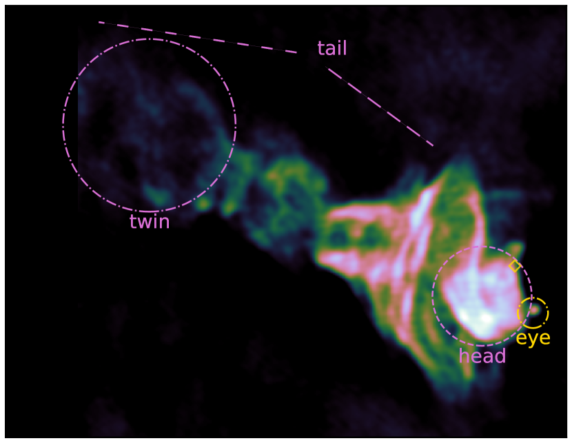
Figure 1: 1.4 GHz VLA continuum image of the Tornado (Brogan & Goss, 2003). The tail, head, and eye are indicated, as well as the X-ray ‘twin’ of the head, detected by Sawada et al. (2011). Like Gaensler et al. (2003), we define the head as the region from which both X-ray and radio emission are strongly detected. The gold diamond indicates the location of an OH (1720 MHz) maser.

Known as ‘the Tornado’, G357.7$-$0.1 (MSH 17-39) is an unusual SNR candidate at a distance of 11.8 kpc (Frail et al., 1996), comprising a ‘head’, ‘tail’, and ‘eye’ (Fig. 1). The head appears as a shell- or ring-like feature in the radio (Shaver et al., 1985), and a ‘smudge’ or diffuse clump with a southern peak in the X-ray, with Suzaku (Sawada et al., 2011) and Chandra (see Fig. 2 of Gaensler et al., 2003) respectively. A larger extended radio shell/filamentary structure exists around the head, with an elongated tail. Finally, a compact and bright radio source seen to the west of the head at $\alpha=17^{\text{h}}40^{\text{m}}05.9^{\text{s}},\delta=-30^{\circ}59^{\prime}00^{\prime\prime}$ (J2000) is the so-called eye of the Tornado, which is an isolated core embedded in a foreground Hii region (Brogan & Goss, 2003; Burton et al., 2004), unrelated to the SNR structure.

Its highly unusual structure has led to various origin theories for the Tornado. From early days, the head of the Tornado has been attributed to a SNR with its radio power law index following synchrotron emission, its non-thermal radio emission, and its strong polarisation (e.g. Milne, 1979; Shaver et al., 1985; Becker & Helfand, 1985a), and later its X-ray emission power-law index (Yusef-Zadeh et al., 2003; Gaensler et al., 2003). These properties led Gaensler et al. (2003) to propose that the Tornado is a shell or mixed morphology SNR, as described by Rho & Petre (1998). The radio head of the Tornado (which is brightest in the south-west part of the ‘shell’ with a peak in the north-west) can be attributed to limb brightened emission due to the interaction with a molecular cloud (Gaensler et al., 2003). Indeed, shocked $\rm H_{2}$ gas detected along the north-western edge of the head (Lazendic et al., 2004), and the presence of multiple OH masers (Frail et al., 1996; Hewitt et al., 2008) both support this scenario. Unshocked CO emission is found from a cloud to the north-west slightly offset from shocked $\rm H_{2}$, suggesting that there is a dense molecular cloud ($\rm n_{H}\sim 10^{4}-10^{6}\,\rm cm^{-3}$) which could decelerate the shock wave on this side (Lazendic et al., 2004). However, it is difficult to explain the shape of the large filamentary structures in the tail (Fig. 2) with a mixed morphology SNR. In this scenario, the X-ray emission from the head (detected with Chandra) originates from the SNR interior, i.e. interior to the limb brightened radio shell (Gaensler et al., 2003). Outside the head region, Shaver et al. (1985) suggests that the partial helical/cylindrical radio filaments could be the result of an equatorial supernova outburst, or the SN exploded at the edge of dense circumstellar shell (Gaensler et al., 2003), or a pre-existing spiral magnetic field structure (Stewart et al., 1994).

Another explanation is that the helical tail is a structure originating from jets of an X-ray binary, as seen in the SNR W50 (Shaver et al., 1985; Helfand & Becker, 1985; Stewart et al., 1994). In that system, over the course of 20 kyr and several episodes of activity, precessing relativistic jets of the X-ray binary SS443 have shaped the SNR within which it is found (e.g. Begelman et al., 1980; Goodall et al., 2011). This has resulted in a huge nebula (208 pc across) which has a circular radio shell (with a 45 pc radius) from the expanding SNR, and lobes extending to 121.5 and 86.5 pc to the east and west respectively formed by outflows. Radio observations of the Tornado show some symmetry, with flared ends and a narrower central region (Caswell et al., 1989), and Sawada et al. (2011) suggested the presence of an X-ray ‘twin’ to the head at the far end. This has lead to the theory that the Tornado is an X-ray binary, with a powering source near to the centre of the radio structure, and bipolar jets which interact with ISM at either end, forming the head and its ‘twin’.

However, a compact object powering the Tornado system has not yet been detected (Gaensler et al., 2003), although Sawada et al. (2011) argued that a central powering source with an active past may now be in a quiescent state and is too faint to detect in X-ray emission. Another proposed idea is that the Tornado is a pulsar wind nebula powered by a high-velocity pulsar (Shull et al., 1989); however, the spectral slope required to explain the X-ray emission is too steep (Gaensler et al., 2003). Currently, the origin of the highly unusual shaping observed in the Tornado is still under debate.

SNRs are considered to play an important role in the dust processes in the ISM, by creating freshly formed ejecta dust and destroying pre-existing interstellar dust. Indeed, dust thermal emission is widely detected in SNRs in the mid- and far-infrared (MIR and FIR) regime (Dunne et al., 2003; Williams et al., 2006; Rho et al., 2008; Barlow et al., 2010; Matsuura et al., 2011; Temim et al., 2012; Gomez et al., 2012; De Looze et al., 2017; Temim et al., 2017; Rho et al., 2018; Chawner et al., 2019; De Looze et al., 2019). As SNRs plough through surrounding interstellar dust clouds, they form a shell-like structure, whereas ejected material is found in a compact emission source in the center of the system (Barlow et al., 2010; Indebetouw et al., 2014). Using MIR to FIR images of the region from the Spitzer Space Telescope (Spitzer, Werner et al., 2004) and the Herschel Space Observatory (Herschel, Pilbratt et al., 2010), Chawner et al. (2020) reported the discovery of thermal emission from dust in the head and tail of the Tornado (see Section 2). This paper examines the unusual morphology of dust emission in the SNR candidate, the Tornado.

2 The Infrared View of the Tornado

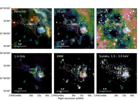
Figure 2: G357.7$-$0.1, The Tornado at FIR, radio, and X-ray - top left: Herschel three colour image made by combining the 70 (blue), 160 (green) and 250 $\mu$m (red) images, top middle: Herschel 70 µm image, top right: Spitzer MIPS 24 µm image, bottom left: 1.4 GHz VLA image, bottom middle: XMM-Newton X-ray image smoothed to 0.5^′′ pixels (kindly provided by B. Gaensler et al. private communication), and bottom right: Suzaku 1.5 – 3.0 keV X-ray smoothed continuum image. The white contours show the radio emission (1.4 GHz VLA) and the cyan contours show X-ray emission (XMM-Newton). We detect dust emission across all Herschel wavebands from the ‘head’ of the Tornado, within the pink circle. We also detect FIR emission from the ‘tail’ of the Tornado, and from a fainter filament extending around the head, as indicated by the arrows. The gold diamond indicates the location of an OH (1720 MHz) maser. (For the single wavelength panels we use the cubehelix colour scheme, Green (2011).)

2.1 Observations

The Herschel data used to discover dust emission in the Tornado is from the HiGal survey (Molinari et al., 2010, 2016), which covered $360^{\circ}$ in longitude and $\mid b\mid\leq 1$ and includes data from 70 – 500 $\mu$m. Data processing is described in detail in Molinari et al. (2016) and pipeline-reduced and calibration corrected fits files are available to the community via the native HIPE reduction pipeline. Zero-point calibrations for the Herschel SPIRE observations were already applied prior to data acquisition. The Herschel PACS zero-point offsets were corrected by comparing the observations to synthetic observations produced from the Planck foreground maps (Planck Collaboration, 2016), and the 100 µm IRAS  IRIS data. This method is similar to that described in e.g. Bernard et al. (2010); Lombardi et al. (2014); Abreu-Vicente et al. (2016). Spitzer 24 µm data was available via the IRSA archive. The MIR-submm images of the Tornado are presented in Fig. 2 (and Fig. 12), where the well known features are marked by a magenta circle (the head), arrows (the tail) and a gold circle (the Hii region, the eye). The tail is brightest in two prong-like structures east of the head.

Fig. 2 also compares the IR images with other physical tracers. We make use of the 1.4 GHz VLA radio image (with spatial resolution of $14^{\prime\prime}\times 11^{\prime\prime}$, Brogan & Goss 2003) and X-ray data from the EPIC camera on board XMM-Newton (kindly provided by B. Gaensler et al. private communication), with an energy range 0.15-15 keV and spatial resolution of $6^{\prime\prime}$. As the source was only weakly detected in the EPIC MOS detector, here we present data from the PN detector only. We use XMM-Newton rather than Chandra as we are only interested in the comparison of structures rather than absolute flux or spectral variations. Furthermore, the diffuse source concentrated at the south of the head previously detected with Chandra (Gaensler et al., 2003) is very faint and requires significant smoothing to bring out the signal; XMM-Newton may ultimately be more sensitive to diffuse emission given its coarse angular resolution compared to Chandra. X-ray observations from Suzaku (Sawada et al., 2011) suggest faint diffuse X-ray emission across the head of the Tornado, in close agreement to the structures observed in the XMM-Newton image (Fig. 2). We note that the distribution of X-rays as seen in the XMM-Newton image suggest a shell-like X-ray structure with some emission in the south which may lie interior to the shell (i.e. potentially originating from ejecta; see also the peak in the smoothed Chandra image of Gaensler et al., 2003).

2.2 Comparison of Tracers

Although this region is confused by dust in the interstellar medium (ISM) in the FIR, we detect clear emission from dust at the location of the head and tail of the SNR in all Herschel wavebands, as shown in Fig. 2 and Fig. 12, though the poorer resolution at 350 and 500 µm makes it more difficult to distinguish the emission from unrelated structure along the line of sight. At 70 and 160 µm, the shell-like structure is clearly seen in the head, and correlates spatially with the radio and overlaps with X-ray. This is also confirmed in the Spitzer 24 $\mu$m image (Fig. 2). The brightest peak in the MIR and FIR (to the north and north-west) is opposite to that seen in the radio emission, and is located towards the OH (1720 MHz) maser, where shock-heated $\rm H_{2}$ is also bright (Lazendic et al., 2004). This dust feature appears confined within the radio contours, and is significantly brighter than the ambient dust seen further north-west where the interacting IS cloud is located (as traced by molecular CO emission; Lazendic et al., 2004) so there is no doubt that this is associated with the emission structures responsible for the radio and X-ray (i.e. shocked gas). The fainter southern peak in the X-ray emission correlates with two radio peaks, and the bright X-ray feature to the west coincides with the brightest 24 $\mu$m emission and fainter radio.

Outside of the head, we detect warm dust in the unrelated Hii region. We also detect faint 70 µm emission that appears to correspond to one of the large radio filaments extending around the eastern side of the head. Dust emission from the tail is also seen at 24 – 160 $\mu$m. Similar to the head, we see evidence of an anti-correlation between the radio and FIR in the tail, the FIR correlates with the upper, fainter of the two radio prongs, indicated by an arrow in Fig. 2. At longer Herschel wavelengths, we see a bright structure at the eastern end of the tail which may be associated with the Tornado, although this is difficult to distinguish from interstellar dust due to the level of confusion in this region. We do not discuss this source further.

3 Investigating the dust structures in the Tornado

In the previous Section, we discussed the presence of dust in the SNR G357.7-0.1, ‘the Tornado’ (Fig. 2). Here we investigate the dust properties in this source further using the point process mapping technique, ppmap. This technique produces maps of differential dust column density for a grid of temperatures (Marsh et al., 2015; Marsh et al., 2017). Observations are taken at their native resolution, avoiding data loss through degrading to a common angular scale, and are deconvolved with circularly average instrument beam profiles, using the point spread function information, to achieve maps of dust mass at a high resolution. Finely sampled colour corrections, derived from the Spitzer MIPS and Herschel PACS and SPIRE response functions, are applied to the model fluxes, as a function of temperature and wavelength.

The ppmap procedure is described in full in Marsh et al. (2015); Marsh et al. (2017) and its application to investigating the dust properties in pulsar wind nebulae can be found in Chawner et al. (2019). In brief, ppmap uses an iterative procedure based on Bayes’ theorem to estimate a density distribution of mass in the state space $(x,~{}y,~{}T,~{}\beta)$ where $x$ and $y$ are spatial co-ordinates, $T$ is the dust temperature and $\beta$ is the dust emissivity index (the power law slope that characterises how the dust opacity varies with wavelength). Throughout the procedure, ppmap acts in the direction of minimising the reduced $\chi^{2}$, derived from the sums of squares of deviations between the observed and model pixel values over each local region, after dividing by the number of degrees of freedom. These are estimated by comparing the estimated properties of each tile with a modified black-body model of the form:

$$\centering F_{\lambda}=\frac{M_{\rm dust}B_{\lambda}(T)\kappa_{\lambda}}{D^{2}},\@add@centering$$ (1)

where $F_{\lambda}$ is the flux at a given wavelength, $M_{\rm dust}$ is the mass of dust, $B_{\nu}(T)$ is the Planck function at temperature $T$, $\kappa_{\lambda}$ is the dust mass absorption coefficient, and $D$ is the distance to the source, which is $\sim$12 kpc in this case. The variation of $\kappa_{\lambda}$ at different wavelengths depends on the value of $\beta$ as $\kappa_{\lambda}=\kappa_{\lambda_{0}}(\lambda/\lambda_{0})^{-\beta}$. We adopt $\kappa_{\rm 300}=0.56\rm m^{2}\,kg^{-1}$ (James et al., 2002) in the ppmap analysis.

The process is applied to a multi-band map field to estimate the column density over a range of temperatures. ppmap provides additional information over the standard modified blackbody technique used to derive dust masses because it (i) does not assume a single dust temperature along the line of sight through each pixel, (ii) uses point spread function information to create column density maps without needing to smooth data to a common resolution, and (iii) although it first makes the assumption that the dust is optically thin, it can check this retrospectively. ppmap requires an estimate of the noise levels for each band which describes the pixel-to-pixel variation. Here, this was derived from background subtracted Spitzer and Herschel images using the standard deviation of pixels within apertures placed in quiet regions (minimal variation in foreground emission) near the source. This gives noise estimates of 2.18, 5.47, 11.87, 4.10, 1.72, and 0.48 MJy sr^-1 for the 24, 70, 160, 250, 350, and 500 µm bands respectively, which are assumed to be uniform across the entire map.

3.1 Applying ppmap to the Tornado

We initially selected 12 temperature bins centred at temperatures equally spaced in ${\rm log}(T)$ ranging from 20 to 90 K (guided by our previous analysis of SNRs in C19), we assumed a fixed value for the dust emissivity index, $\beta=2$, which is typical for silicate ISM dust (Planck Collaboration XXXI, 2016). If we were to assume a carbonaceous dust with $\beta$ of 1.0 to 1.5 the estimated dust temperatures would likely be higher. As we did not find any related dust at the location of the head in any temperature bins > 70 K, we re-ran the grid for temperatures ranging from 15 to 70 K.

In our first runs of ppmap, we found that the iterative procedure did not converge to sensible fits (verified by checking the ppmap $\chi^{2}$ statistic in each band), even with hundreds of thousands of iterations. This was due to ppmap attempting, and failing, to converge to a solution for the bright point sources, presumably stars with temperatures much higher than 90 K, in the 24 $\mu$m image (and to a lesser extent in the 70 $\mu$m image). To resolve this, we masked the bright point sources near the Tornado (replacing their pixels with a local average level in the image) and we artificially increased the noise for the 24 $\mu$m map by a factor of 10; this effectively stops ppmap from trying to over-fit the 24 $\mu$m band and down-weights the importance of the 24 $\mu$m in the iterative procedure. This may act to slightly reduce any dust temperatures fit by ppmap, though in practice we found that it did not affect our results.

The Tornado is in a highly confused region due to its location close to the Galactic centre (Fig. 2). To determine the effect of any potential contamination from unrelated dust along the line of sight, we ran our ppmap grid (the original 20 – 90 K run) on the Tornado without any background subtraction, and then again, after accounting for background emission. In the former scenario, the results indicate that dust structures exist in the head of the Tornado at temperatures of 20-23 K with a warmer dust component in the north-western part of the head at 26 K, where the source is believed to be interacting with a molecular cloud (Frail et al., 1996; Lazendic et al., 2004; Hewitt et al., 2008). These cold dust temperatures are very similar to general interstellar dust, and the narrow range of temperatures suggest this region is contaminated by unrelated background emission.

For ppmap to converge in a reasonable time we must subtract the background from the maps. First we mask bright, unrelated sources as above, as well as the Tornado head and tail, and several high signal-to-noise regions to avoid overestimating the background. The images are then convolved with a 100 ^′′ FWHM Gaussian profile, providing background maps smoothed to a scale comparable to the Tornado head. The background maps are subtracted from the original zero-point calibrated maps (with the two bright sources masked). Running ppmap with the resulting maps gives reduced-$\chi^{2}$ values of 0.3, 2.0, 11.0, 9.0, 4.0, and 128.0 for 24, 70, 160, 250, 350, and 500 µm We find that the overall level of the background-subtracted images is negative, implying the method of background subtraction used is too aggressive. To account for this, we took the background-subtracted maps, estimated the mean negative offset for the whole region at each waveband (again masking the Tornado) and added this back on to the image in an attempt to bring the maps back to a zero level. Hereafter we call this the zero mean background-subtracted method. Running these images through ppmap the resulting dust temperatures and components are markedly different to the non-background-subtracted case: dust structures are observed at a wider range of temperatures (from 20 - 60 K) with the north-western dust feature peaking at 30 K. The background subtraction has resulted in the dust components in the head being attributed to warmer dust, as expected. Note that these warmer dust components agree with the dust structures that peak in the original Herschel maps peaking at 70 $\mu$m. The resulting ppmap reduced $\chi^{2}$ values are 0.6, 2.2, 6.9, 11.7, 22.5 and 37.6 suggesting the overall fit is formally better than the previous case. The high $\chi^{2}$ values for the longer wavebands are most likely due to underestimating the $\sigma$ value, because small scale ISM variations cannot be captured by a large beam, although increasing the noise level constrains ppmap less, giving more unreliable results across all bands.

The above tests suggest that ppmap is sensitive to whether the background diffuse interstellar level is subtracted from the maps or not, particularly important in this case due to the high level of confusion in this region. To try and qualitatively discriminate between the tests, we created synthetic MIR-FIR observations based on the ppmap outputs for the three scenarios above, and compared them to the original Spitzer and Herschel images. In each case, the original dust emission features seen in the head of the Tornado were recovered well in the synthetic ppmap MIR-FIR images. The zero mean background-subtracted method provided the closest match to the original features (see Appendix A), recovering the complex dust emission structures observed within the head (see the following Section for more information). We therefore use the ppmap results based on this method from now on.

Finally we note that synchrotron emission in SNRs can be a significant contributor to the FIR flux (Dunne et al., 2003; De Looze et al., 2017; Chawner et al., 2019). As this typically varies as a power law with flux $S_{\nu}\propto\nu^{-\alpha}$ where $\alpha$ is the spectral index, we can directly estimate the contribution of synchrotron emission to our FIR bands. Prior to running ppmap we subtract the synchrotron contribution which is estimated by extrapolating from the flux we measure from the 1.4 GHz VLA image (Becker & Helfand, 1985b; Green, 2004), assuming $\alpha=\,-0.63$ for the head (Law et al., 2008). We find that the synchrotron contribution to the SNR head is in the range of only 0.03 – 2.06 per cent of the total flux for our MIR–FIR wavebands in the head, as measured on the original Herschel maps, where both are measured within an aperture centred at $\alpha\,=\,17^{\text{h}}40^{\text{m}}12.4^{\text{s}},\delta\,=\,-30^{\circ}58^{\prime}31.1^{\prime\prime}$ with a 79^′′ radius. We can therefore be confident that we are observing the thermal emission from dust with negligible contribution from synchrotron emission in the head.

However, the spectral index does flatten in the tail region with spectral slope varying from $-0.50\,<\,\alpha\,<\,-0.33$ (Law et al., 2008) indicating that the tail electrons are more energetic than in the head. We therefore caution that there could be a higher contribution of synchrotron emission in the tail.

3.2 Results

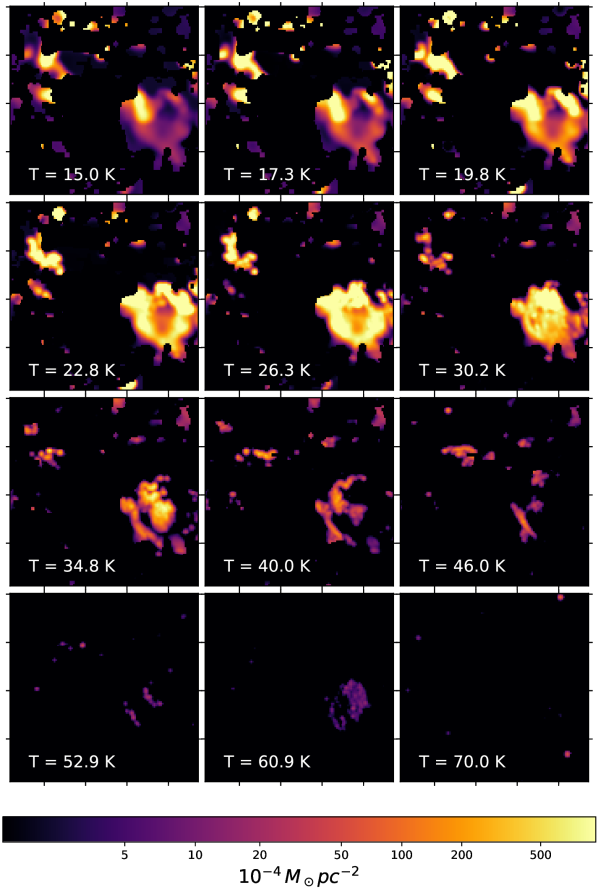
Figure 3: ppmap generated maps of differential dust mass split in different temperature ranges for the Tornado. The corresponding dust temperature is indicated in the bottom-left of each panel.

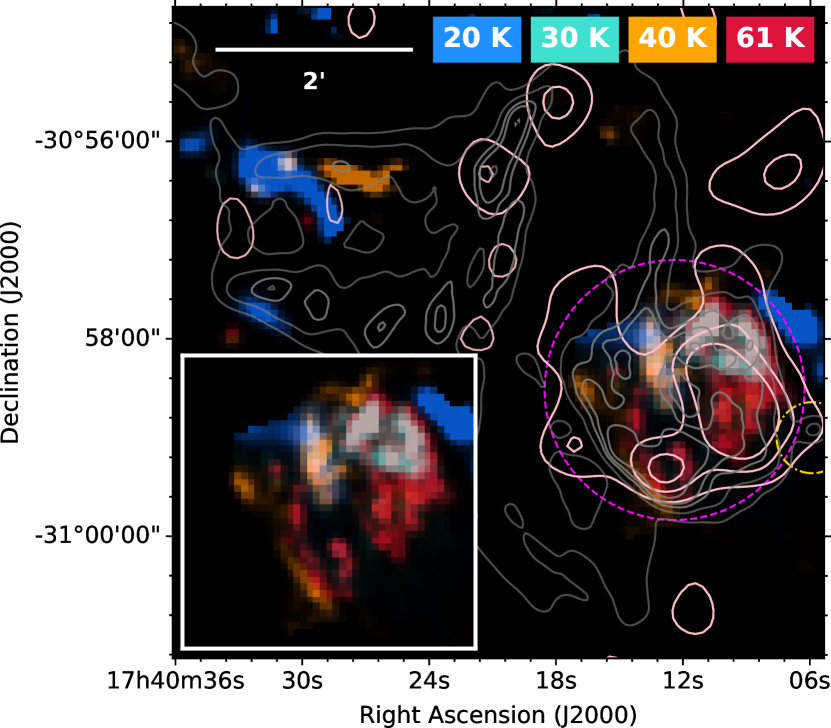
Figure 4: ppmap-generated four colour map of dust mass in the Tornado created using dust temperature slices from Fig. 3. Colours show dust at 20 K (blue), 30 K (cyan), 40 K (gold), and 61 K (red). Overlaid contours are from the VLA 1.4 GHz (grey) and XMM-Newton (pink) images. The magenta dashed circle indicates the location of the head of the remnant, and is also the aperture used to derive the dust mass. The gold dash-dotted circle is the location of the eye of the Tornado (unrelated Hii region).

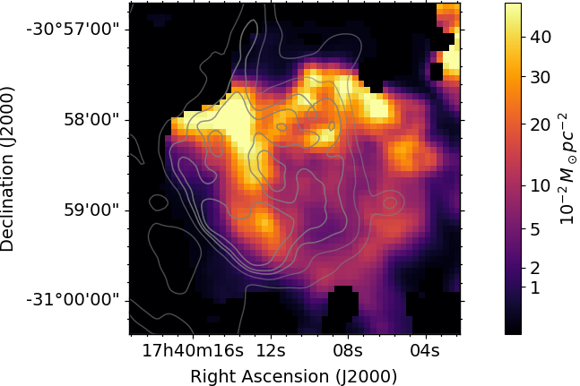
Figure 5: The dust mass within the Tornado head integrated across all temperature slices of Fig. 3, with VLA 1.4 GHz contours (grey) overlaid.

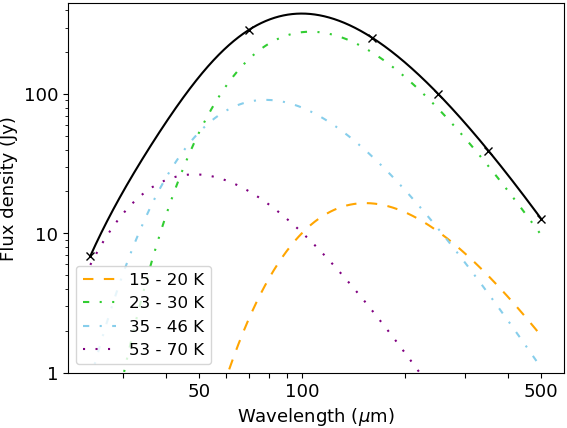
Figure 6: The total thermal MIR-FIR SED estimated from the ppmap results of the head of the Tornado, within the magenta circle in Fig. 4, indicating how the different temperature components shown in Fig. 3 contribute to the thermal emission observed in the source.

The grid of dust mass in each temperature bin for the Tornado is shown in Fig. 3 assuming a distance of 12 kpc (Brogan & Goss, 2003). Fig. 4 shows a four colour FIR image created by combining the masses in the temperature slices at 20, 30, 40, and 61 K, and Fig. 5 shows the total dust mass distribution across the Tornado head. They reveal dust features observed in the Herschel images, but at a resolution of $\sim 8^{\prime\prime}$ compared to the native telescope beams of $5-36^{\prime\prime}$.

A temperature gradient is evident in both the head and tail. Cool, dense dust is found towards the north-eastern head at the location of a radio filament which extends from the head towards the northern extent of the object. The filaments outside of the head were lost in background subtraction, but this suggests that they could also contain cool, dense dust. Slightly warmer material (23 – 30 K) forms a bubble around the edge of the head and around the larger X-ray peak. In Fig. 5 we find that the majority of the dust mass follows this bubble shape, with a relative lack of material in the central region. Warm material (35 – 40 K) fills the central region, coincident with both the large X-ray peak and the warmest dust that we observe (53 – 61 K). It seems that the hot gas which emits the X-ray emission is heating the central region of the head, where we see warm, low density material. We find a large mass of 26 – 30 K dust towards the north west where interactions with a molecular cloud may be heating the dust, as well as at the same location as the smaller region of bright X-ray emission in the south east. A filament of 35 – 46 K material sits along the eastern edge of the head, with a warm 53 K peak towards the middle, filling the radio contours at this location, as seen in Fig.4. In the tail we find a large mass of cool, 15 – 20 K dust to the east, as well as slightly warmer, 23 – 30 K material which extends further north. The temperature increases towards the west, as 35 – 40 K dust fill the eastern and central contours with dense regions at the radio peaks, and 46 K material is found further west. There is some evidence of warm dust (40 – 46 K) at the X-ray and radio peak to the east of the tail, although much of this area is lost to background subtraction as it is a similar level to the surrounding ISM.

The spectral energy distribution of the head of the Tornado is shown in Fig. 6, broken down into the different temperature components revealed by ppmap. We derive the total dust mass in the head of the Tornado by summing the mass within the magenta circle shown in Fig. 4 across the temperature grids. This gives a total dust mass for the Tornado head of 16.7 M_⊙ for a dust mass absorption coefficient at 300 µm of $\kappa_{\rm 300}=$0.56$\,\rm m^{2}\,kg^{-1}$ (James et al., 2002). If we only sum the contribution from dust structures with T_d>17 K we obtain a dust mass of 14.8 M_⊙, and 4.0 M_⊙ of mass originates from dust hotter than $30$K.

4 Dust Grain Properties

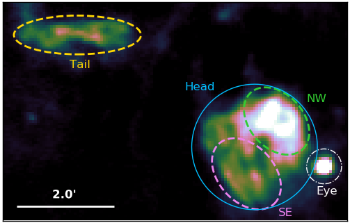
Figure 7: Tornado head and tail region at 70 µm. The shapes indicate regions from which we detect FIR emission and within which we compare the flux ratios in Figs. 9 and 10. These are the Tornado head (blue circle), north-western head (green dashed ellipse, south eastern head (pink dashed ellipse), Tornado tail (gold dashed ellipse), and the Tornado eye (white dash-dotted circle).

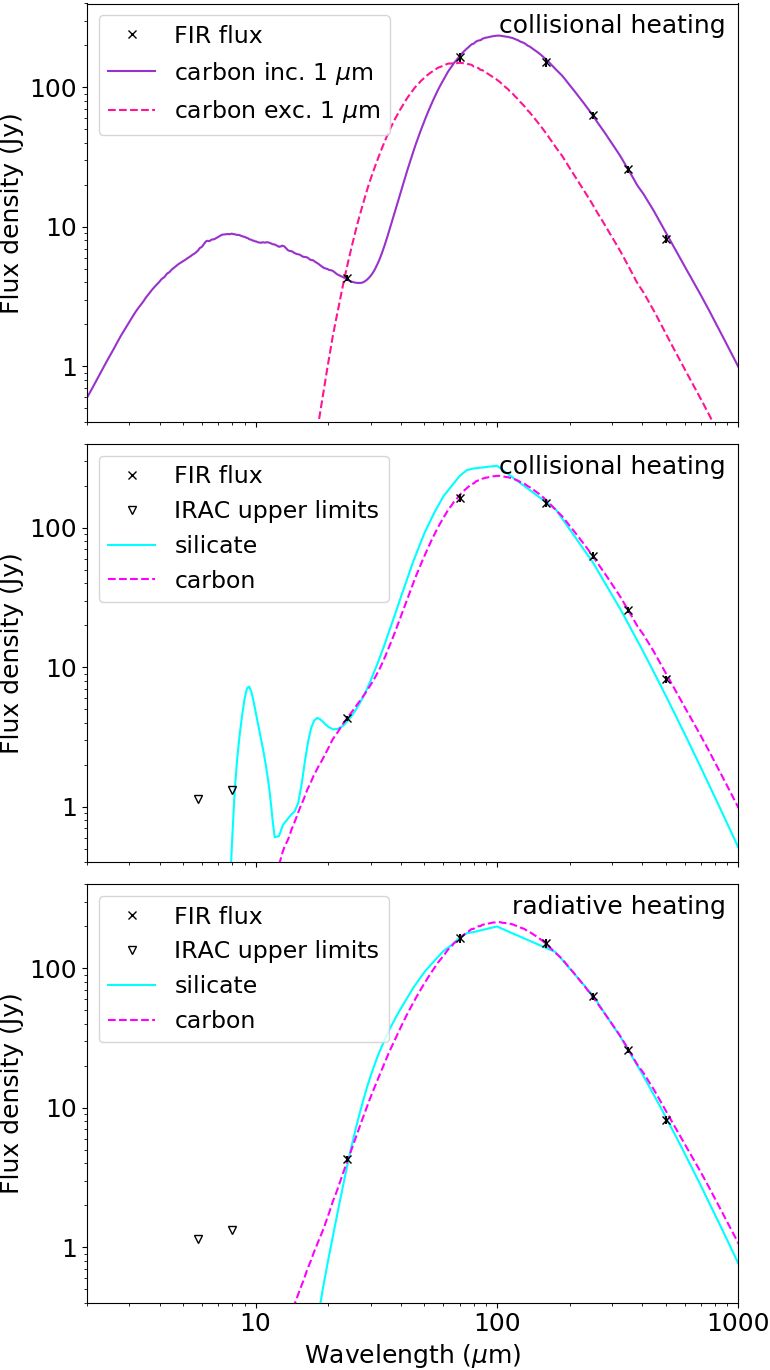
Figure 8: Best-fit dust SEDs for the Tornado head assuming that dust is collisionally heated by hot gas in the top two panels, and radiatively heated in the bottom panel. We use DINAMO (Priestley et al., 2019) to fit to the flux within the head aperture in Fig.7, assuming the gas properties estimated by (Sawada et al., 2011). Although we can fit the SED well to the measured FIR fluxes with a collisional heating model and carbon grains, this requires a highly unusual grain size distribution. It is more likely that the majority of the dust within the Tornado head is radiatively heated, with a small proportion of collisionally heated dust.

In previous investigations both Sawada et al. (2011) and Gaensler et al. (2003) detected thermal X-ray emission from the head of the Tornado. This led Gaensler et al. (2003) to suggest that the head is a mixed-morphology SNR, centrally filled with thermal X-ray emission from shocked gas. In Figs. 3 and 4 we find that the warmest dust ($\sim$60 K) is at the location of the XMM-Newton X-ray peak, thus we investigate whether the dust in the head is likely to be collisionally heated by hot, shocked gas.

We calculate grain temperatures and corresponding emissivities for grain sizes between 0.001 – 1 µm using DINAMO (Priestley et al., 2019), a dust heating code which takes into account temperature fluctuations of small grains. We assume that the dust is heated by gas with the properties measured by Sawada et al. (2011) ($kT=0.73$ keV and $n_{e}=0.49$ cm^-3), and use optical properties for either BE amorphous carbon (Zubko et al., 1996) or MgSiO₃ grains (Dorschner et al., 1995). The corresponding opacities at 300 µm are 0.79 m²g^-1 and 0.32 m²g^-1 ($\beta=$ 1.5 and 1.7) respectively. The minimum equilibrium grain temperature, for micron-sized grains of either composition, is $\sim$30 K, so no set of grain properties result in an emissivity resembling a 20 – 30 K blackbody, as indicated by PPMAP.

Following the method used in (Priestley et al., 2020), we fit the IR SED to background-subtracted fluxes within the blue head aperture in Fig. 7 using a combination of single-grain SEDs for radii of 0.001, 0.01, 0.1 and 1 µm  with the number of grains (or equivalently the dust mass) of each size as the free parameters. We are unable to fit the FIR fluxes if we exclude 1 µm grains. For carbon grains, shown in the top panel of Fig. 8, even 0.1 µm grains have a 24/70 µm ratio which is larger than the observed value, while at longer wavelengths the discrepancy becomes even more extreme. Silicate grains have the same issue, to a slightly greater extent. With 1 µm radius grains included, we are able to reproduce the SED well at all wavelengths. We include IRAC fluxes (which may have significant non-SN dust contamination) as upper limits, in order to better constrain the number of transiently heated small grains, and we find best-fit dust masses of 8.1 M_⊙ for carbon grains and 17.3 M_⊙ for silicates. The best-fit SEDs are shown in Fig. 8.

In order to fit the FIR fluxes, both carbon and silicate grains require the vast majority ($\sim$99 per cent) of the dust mass to be in micron-sized grains, while also requiring 0.05 – 0.06 M_⊙ of small grains with $a\leq$0.01 µm to reproduce the 24 µm emission. The mass of intermediate-sized grains with radius 0.1 µm is strongly constrained to be below 10^-4 M_⊙, where they have a negligible contribution to the total SED. This distribution of grain sizes is highly unusual, both for the high mass fraction of micron-sized dust - the Mathis et al. (1977) power law does not extend to 1 µm  and even if extended results in only $\sim$30 per cent of the mass in the largest grains - and the ‘bimodal’ distribution of small and large grains. Additionally, assuming a gas to dust ratio of 100, a dust mass of $\sim$10 M_⊙ implies a gas mass of $\sim$1000 M_⊙, much larger than that indicated by the X-ray emission (M${}_{gas}=$23 M_⊙, Sawada et al., 2011). We consider it more probable that the assumption of all grains being heated by the X-ray emitting gas is wrong. The synchrotron radiation generated by the shocked gas will heat nearby grains, both in the unshocked ISM and in any local over-densities which survive the blast wave, potentially resulting in a population of grains at lower temperatures.

While fully investigating the potential range of spectral shapes and intensities is beyond the scope of this paper, we can approximate it by scaling the Mathis et al. (1983) radiation field by a constant factor G. Assuming that the radiatively heated dust follows an MRN size distribution, we are able to fit the SED without the addition of micron-sized grains for G = 5 for carbon and 10 for silicates. The best-fit SEDs, shown in Fig. 8, require 9.1 M_⊙ and 0.33 M_⊙ of radiatively and collisionally heated dust respectively for carbon grains. The size distribution of the collisionally heated dust is also reasonable, with the majority of the mass at 0.1 µm and a negligible fraction of 0.001 µm grains, as would be expected from an initial size distribution affected by sputtering (Dwek et al., 1996). For silicates, the radiatively and collisionally heated dust masses are 35.7 and 0.76 M_⊙ respectively. We note that these dust masses are not authoratative - differences in the assumed grain properties, size distribution and radiation field could cause significant variation in the best-fit masses. However, it is clear that a moderately-enhanced radiation field in the vicinity of the Tornado, combined with a small mass of dust in the shocked plasma, can explain the observed IR SED without any additional assumptions. Our G = 6 carbon model has a total cold dust luminosity of 2.6$\times$10³⁷erg s^-1 which can be explained by radiative heating via synchrotron radiation from the shock wave, given $\alpha=-0.63$ (Law et al., 2008). We consider this explanation much more reasonable than invoking an arbitrary, and somewhat unphysical, size distribution for the dust in the hot plasma. Investigations of the IR-X-ray flux ratio may give a more detailed description of the processes within the Tornado head, as shown for other SNRs by Koo et al. (2016), although possible absorption by dense gas and molecular material in the vicinity makes this complicated.

In Section 3.2 we estimated that the head of the Tornado contains a large dust mass of 16.7 M_⊙. This is unexpected for the mass within a SNR. However, if the Tornado head is a SNR, it will have swept up a large mass of dust from the ISM through expansion. Assuming a simple relation where the swept up mass is equal to $\frac{4}{3}\pi R^{3}\rho$, with a standard ISM density for cool, dense regions of $\rho=10^{-21}$ kg m^-3, this gives a mass of $\sim 5.26$ M_⊙. As the ISM in this region is expected to be relatively dense, the swept up mass will likely be larger than this; assuming a gas density of $10^{4}$ cm^-3 (Lazendic et al., 2004) and dust-to-gas ratio of 100, the total swept up dust mass could be as large as $\sim$250 M_⊙. Therefore, the dust mass of the Tornado head can be explained by material which has been swept up by an expanding SNR.

5 The Nature of the Tornado

The nature of the Tornado is unclear as it has many confusing characteristics, with suggested candidates including an X-ray binary, a SNR, and Hii region. In Section 3 we revealed that the Tornado contains large masses of dust, similar to the sandy whirlwind ‘Dust Devils’ on Earth. In this section we explore whether the FIR emission from our own Dust Devil can give us any insight into its nature. We further examine the IR, radio, and X-ray emission to determine if it can shine any light on the different origin scenarios.

5.1 Properties of the Tornado

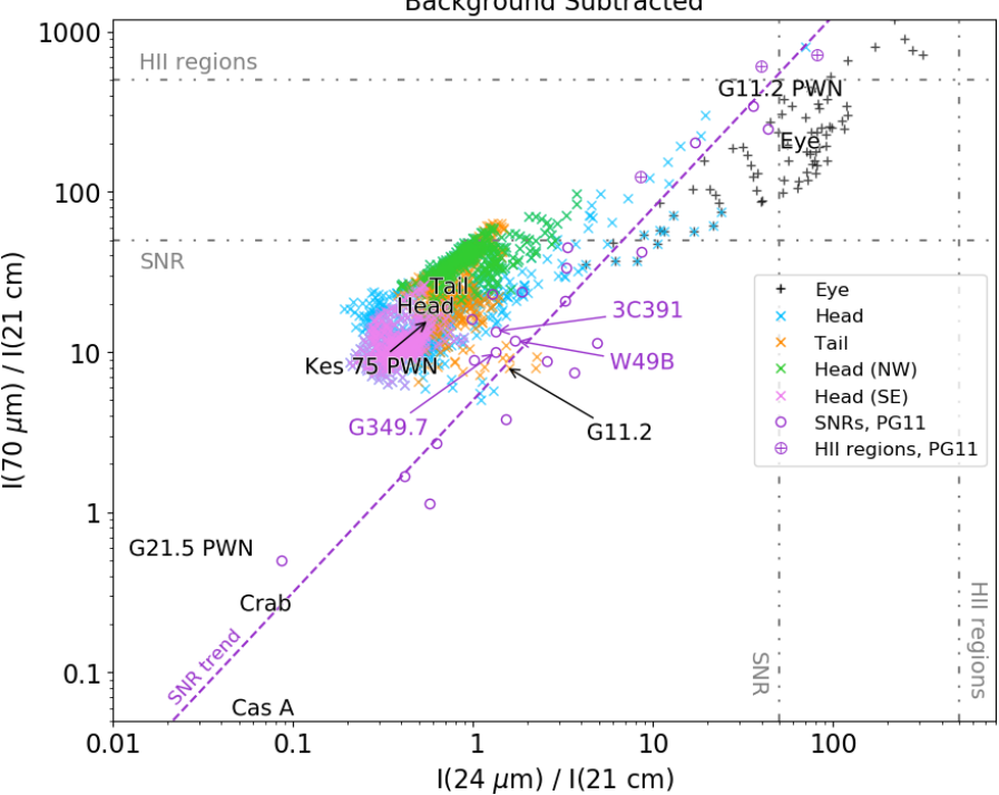
Figure 9: Flux ratio of individual pixels and integrated flux within the Tornado head, eye, and tail (within the circled regions in Fig. 7), in comparison with other SNRs and Hii regions. Pixels with very low signal have been removed, where the signal divided by the subtracted background is <0.1. The fluxes for the NW and SE head, and the tail are measured from the regions indicated in Fig. 7. The text labels are centred on the integrated flux for the Tornado head and eye, and previously studied SNRs, estimated by De Looze et al. (Cas A and Crab; 2017, 2019) and Chawner et al. (G11.2, G21.5, G29.7 and G351.2; 2019, 2020). The grey dashed-dotted lines indicate ratios of 50 and 500, used in previous studies as diagnostics of SNRs and Hii regions. The majority of the Tornado head and tail pixels fall within the SNR region, and are clearly different to the pixels within the eye, which sits very close to the Hii region area of the colour space. All regions of the Tornado are found towards the upper right of the SNR regions, suggestive of an older remnant. There is a noticeable variation in the flux ratio of the NW and SE regions of the head.

Figure 10: Flux ratio of individual pixels within the head, eye, and tail of the Tornado (within the circled regions in Fig. 7), in comparison with other SNRs and Hii region. Pixels with very low signal have been removed, where the signal divided by the subtracted background is <0.1. The fluxes for the NW and SE head, and the tail are measured from the regions indicated in Fig. 7. The text labels are centred on the integrated flux for the Tornado head and eye, and previously studied SNRs, estimated by De Looze et al. (Cas A and Crab; 2017, 2019) and Chawner et al. (G11.2, G21.5, G29.7 and G351.2; 2019, 2020). We also include ratios for SNRs with known molecular interactions, atomic fine-structure emission, and PDRs from Pinheiro Goncalves et al. (2011). The purple dashed and the grey dash-dotted lines indicate SNR and Hii region trends respectively, found by Pinheiro Goncalves et al. (2011). SNRs populate a wider area in this colour space and several Pinheiro Goncalves et al. (2011) SNR measurements lie along the Hii region trend, including those highlighted in pink text. The grey dotted lines show the flux ratios expected from a thermal source with $\beta=2$ and the temperature indicated. The Tornado is found towards the upper right of this colour space, suggestive of an older remnant. It is also found in a region populated mainly by SNRs with molecular interactions.

First, we study the emission colours to understand the properties of the regions from which we detect dust and how they vary across its features. Within the head, we split our analysis into two main regions of interest, as indicated by the green and magenta ellipses in Fig. 7 respectively: the north-west (NW), where we identified warm dust with ppmap and where the head is thought to be interacting with a molecular cloud (Frail et al., 1996; Lazendic et al., 2004; Hewitt et al., 2008), and the south-east (SE), where there is a radio peak. Our PPMAP analysis in Section 3 gives estimates for the dust mass within each of these regions as $\sim 3.3M_{\odot}$ and $\sim 2.1M_{\odot}$ for the NW and SE respectively.

IR – radio flux ratios have been used in previous studies to identify SNRs, distinguishing from Hii regions (e.g. Whiteoak & Green, 1996). The thermally dominated emission from Hii regions, with some free-free emission in the radio, gives an IR-radio ratio of $\geqslant$ 500; in contrast, SNRs are dominated by synchrotron at radio frequencies and have a considerably smaller IR flux, giving an IR - radio ratio of $\leqslant$ 50 (Haslam & Osborne, 1987; Furst et al., 1987; Broadbent et al., 1989).

In order to examine the dust emission properties of the various FIR regions of the Tornado, we follow the analysis of Pinheiro Goncalves et al. (2011) and compare IR and radio colours, including $I_{\rm 70\mu m}/I_{\rm 21cm}$, $I_{\rm 24\mu m}/I_{\rm 21cm}$, $I_{\rm 8\mu m}/I_{\rm 24\mu m}$ and $I_{\rm 70\mu m}/I_{\rm 24\mu m}$, for pixels within the Tornado (Figs. 9 and 10), where pixels are convolved to the lowest resolution data. For comparison we include the integrated flux of the head, the dusty region in the tail (see Fig. 7), the eye, and previously studied SNRs (in Figs. 9 and 10 the SNR and region names are centred on the respective flux ratios, unless indicated by an arrow).

In Fig. 9 we find that the IR colours for the majority of the Tornado head pixels fall within the colour space for a SNR, and are well distinguished from the pixels within the ‘eye’ of the Tornado, which is a confirmed Hii region with an embedded protostellar source (Burton et al., 2004). This suggests that the Tornado head is part of a SNR, rather than a Hii region. Several Galactic SNRs from Pinheiro Goncalves et al. (2011) are observed to have high IR-radio flux ratios, two of which would be classified as Hii regions by this test ($I_{\rm IR}/I_{\rm radio}>500$: G21.5$-$0.1 and G23.6$+$0.3, $I_{\rm IR}/I_{\rm radio}>50$: G10.5$+$0.0, G14.3$+$0.1, G18.6$-$0.2, and G20.4$+$0.1). Of these sources, Anderson et al. (2017) suggested that three were misidentified Hii regions (G20.4, G21.5, and G23.6), which we have labelled in Figs. 9 and 10.

As shown in Fig. 10, Pinheiro Goncalves et al. (2011) found different trends for Hii regions and SNRs when comparing their IR colours. In this colour space, we find that the Tornado falls more in line with the Hii region trend. However, SNRs and Hii regions inhabit much of the same colour space in Figs. 9 and 10 and there are other well known SNRs, including W49B, 3C391, and G349.7$-$0.2, which also lie along the Hii region trend. The variation seen in these individual SNRs from the main SNR trend could instead be due to a difference in dust properties such as temperature or emissivity, possibly caused by interactions with molecular clouds.

It is possible to use the IR and IR – radio colours, as in Figs. 9 and 10, to determine some of the SNR properties. Older SNRs tend to have higher IR – radio colours (e.g. Arendt, 1989), placing them towards the upper-right of the SNR colour space in Fig, 9. Additionally, Pinheiro Goncalves et al. (2011) found some correlation between the IR colours in Fig. 10 and the SNR age, suggesting that older remnants have higher 70 – 24 µm and 8 – 24 µm flux ratios. Thus, both the FIR – radio and the IR colours suggest that, if it is a SNR, the Tornado is an older remnant which has likely swept up a large mass of dust from the ISM. Pinheiro Goncalves et al. (2011) also suggested that the IR colours could give some insight into the SNR emission process. They found tentative evidence that the upper right region of the colour space in Fig. 10 tends to be populated by objects with molecular shock and photodissociation regions (PDRs), although they admit that this is not a secure correlation given the small sample and that the 8, 24, and 70 µm bands may contain both dust emission and lines. We find that the IR flux ratios of the NW region of the Tornado Head suggests molecular emission, whereas the SE region is largely undetected at 8 µm. Given that the head is thought to be interacting with a molecular cloud in the NW, this supports the relation between the 70 µm – 24 µm and 8 µm – 24 µm flux ratios and emission type.

In all of the colour plots we find that the NW and SE regions (Fig.7) of the head are distinct and must have different emission processes. Fig. 9 shows a higher FIR – radio flux ratio in the NW region, suggesting an increased amount of thermal emission in the same area in which we see warm dust in Fig. 3: this dust may be heated through an interaction on this side.

5.2 What the Devil is it?

Gaensler et al. (2003) found that the X-ray emission from the head can be well explained by thermal models, rather than synchrotron emission, with a gas temperature of $kT\sim 0.6$ keV, arising from the interior of a limb-brightened radio SNR. Indeed, in Fig. 4 we find that the warmest dust is coincident with X-ray emission in the central region where hot gas may be heating the dust, as expected for a mixed-morphology SNR (Rho & Petre, 1998; Yusef-Zadeh et al., 2003). Sawada et al. (2011) estimated an X-ray temperature of 0.73 keV for the head. Using an X-ray temperature of 0.73 keV (T = 8.6 where T is in a unit of 10⁶ K) and assuming that the Tornado nebula is an SNR, we estimate a shock velocity (V_s) and age ($t$) of the SNR using the radius of only the head and both the head and tail (1.3^′ and 5.4^′). The shock velocity is 884 km/s based on $V_{s}=(T/11.)^{0.5}\times 1000$ kms^-1 (Winkler & Clark, 1974). The age of the SNR ($t=2/5Rs/Vs$) is therefore between 2000 and 8000 yr.

The bizarre shape of the tail is more difficult to explain with a SNR scenario. Gaensler et al. (2003) suggested the tail could be explained by a progenitor star moving across the space whilst losing mass, which then exploded as a SN at the edge of circumstellar material (CSM; Brighenti & D’Ercole, 1994). A similar scenario has been suggested for the SNR VRO 42.05.01 (G166.0$+$4.3, Derlopa et al., 2020) which is much larger than the Tornado but morphologically resembles the Tornado head and surrounding filaments. When a progenitor star moves in relatively higher density interstellar medium (ISM), the stellar motion could cause a bow shock at the site of interaction between CSM and ISM. Bow shocks have been detected in the red-supergiants $\alpha$ Ori and $\mu$ Cep (Noriega-Crespo et al., 1997; Martin et al., 2007; Ueta et al., 2008; Cox et al., 2012). In the former, the bow shock has a wide opening angle, whereas the latter has a narrow-angle cylinder-type bow shock. The cylinder shape of the Tornado’s tail could therefore be explained by CSM-ISM interaction. However, the CSM from red-supergiants does not emit synchrotron emission, so that the radio emission observed in the Tornado’s tail would require additional energy by the SN-CSM interaction. This requires the SN explosion itself to be highly elongated with very fast blast winds towards the east by more than by a factor of 10 to the west, which is unlikely and not supported by the hydrodynamic model (Brighenti & D’Ercole, 1994). Instead of synchrotron, the radio tail emission could be free-free; however, in that case, there should be some major heating and an obvious ionising source in the tail, which we do not see in the Spitzer 24 $\mu$m image (Fig. 2). Instead of a red-supergiant, the progenitor star could be a Wolf Rayet (WR) star, which has ionised gas in the CSM, and hence can emit free-free emission at radio wavelengths. However, the lifetime of a WR star is too short to form such a large scale structure while the star is moving in the local space. The typical lifetime of a WR star is 10 – 36 kyrs (Meynet & Maeder, 2003, 2005). At a distance of 12 kpc, the furthest filament (centred at approximately $\alpha=17^{\text{h}}40^{\text{m}}43.8^{\text{s}},\delta=-30^{\circ}55^{\prime}44.9^{\prime\prime}$) is $\sim 25$ pc from the centre of the Tornado head. This requires a progenitor to move through the ISM at speeds of approximately 1,000 km s^-1. Though not impossible, such a high speed motion is unlikely. It is therefore difficult to explain the Tornado’s tail with past mass loss from a SN (SN-CSM interaction).

Although the X-ray and radio emission from the head can be explained by thermal and synchrotron radiation from a SNR, the presence of an X-ray binary within the SNR would explain the length and the morphology of the tail in radio emission (Helfand & Becker, 1985; Stewart et al., 1994). Stewart et al. (1994) detected a spiral magnetic field around both the head and tail which they proposed could be explained by outflows from the central source dragging existing fields along the precession cone. In this instance, thermal X-ray emission at the location of the head is expected to arise from interactions between the jets and surrounding nebula, similar to that seen in the X-ray binary SS433 surrounded by the SNR W50 (Brinkmann et al., 1996; Safi-Harb & Ögelman, 1997). The radio power law index of the central part of W50 is found to be typical for SNR ($\alpha\sim$0.58, Dubner et al., 1998), while a hydrodynamic model shows that episodic jets from an X-ray binary containing a black hole compresses the SNR shell, forming a cylinder/helical shaped outflow in one direction (Goodall et al., 2011).

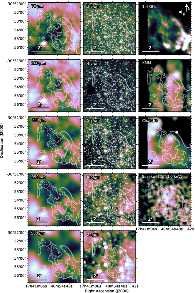
Figure 13: IR, radio, and X-ray view of the location of the X-ray twin, detected by Sawada et al. (2011), the scale is increased compared with the image in Fig 2 to enhance any features in the region. Left column: Herschel images, middle column: Spitzer images, right top: 1.4 GHz VLA image, right second row: XMM-Newton X-ray image, right third row: Chandra X-ray image, and right bottom: Suzaku 1.5 – 4.0 keV X-ray image. We note that we have not applied a background subtraction or correction for vignetting as was done by Sawada et al. (2011). The white contours show the VLA 1.4 GHz emission. In all Herschel and IRAC bands the flux level at the location of the twin is similar to, or lower than, that of the surrounding ISM. In all other bands there is some emission, although the morphology is not consistent with the Suzaku features, and at 24 µm this is fainter than much of the surrounding ISM. (We use the cubehelix colour scheme, Green (2011).)

If the Tornado is formed by a binary system, the location of its source is controversial. In the case of the W50 – SS433 system, the high mass X-ray binary is located in the SNR, following which would place the Tornado binary within the head. However, Sawada et al. (2011) suggested that there is a Suzaku 1.5 – 3.0 keV band detection of a ‘twin’ source, opposite to where X-ray emission is already detected in the Tornado head. They propose that this originates from the interaction between the second jet of an X-ray binary system and a molecular cloud, placing any potential binary system source at the middle of the structure seen in Fig. 2, rather than in the head. In this case, one might expect visible emission in the IR/FIR wavelengths at the location of the ‘twin’ due to shocked gas/heated dust arising from jet interaction with the ISM. In the 24 µm and the Herschel bands there is emission towards the south-west of this region which correlates with radio structures in the tail. However, we do not see any clear evidence for an IR counterpart of the ‘twin’: in all Spitzer and Herschel maps the flux at the location of the Suzaku peak is at a similar level to, or lower than, that of the surrounding area (see Fig. 13). There is some X-ray emission in the XMM-Newton and Chandra data at the location of the ‘twin’, although the emission does not seem correlated. However, the X-ray emission may be affected by foreground absorption, making association difficult to determine, and the region may peak in the 1.5 – 3.0 keV Suzaku band with much lower emission of softer X-ray, making comparison between multiple bands complicated.

As there does seem to be X-ray and radio emission at the location of the ‘twin’ it is plausible that there is an object in this region, which may be associated with the Tornado as suggested by Sawada et al. (2011). However, if there is emission from such an object in any of the Spitzer or Herschel bands, it is very faint and is not detected above the level of the ISM in this region (Fig. 13). This is unlike the head, from which there is a clear detection in the 5.8 – 500 µm bands, as well as a very bright radio structure (Fig. 12). It seems strange that their IR profiles are so different if the two regions have been formed by a similar process, although we cannot exclude this as a possibility. If the X-ray ‘twin’ head is unrelated to the Tornado, it is plausible that the location of an X-ray binary, if any, could be within the head of the Tornado as discussed above.

Although the IR-radio emission supports a SNR origin for the Tornado head, we see no clear indication that the X-ray emission from the head results from an interaction between X-ray binary jets and the surrounding nebula. However, the helical shape of the tail, and the presence of its magnetic field and synchrotron radiation, can be explained by a jet ploughing into a SNR shell, as observed in W50. Although there is no detection of a central powering source, there are cases in which the central X-ray binary may be too faint to detect at a distance of 12 kpc. Gaensler et al. (2003) suggest that this would be the case for a high-mass X-ray binary such as LS 5039 (Paredes et al., 2000), from which the luminosity may vary with orbital phase and its minimum is slightly higher than the upper limit for detection of a Tornado central source. It could also be the case that the Tornado is powered by a low mass X-ray binary in a quiescent state, having produced the observed features in a past period of prolonged activity (Sawada et al., 2011), as seen in 4U 1755–338 (Angelini & White, 2003).

6 Conclusion

We detect FIR emission from dust in the unusual SNR candidate the Tornado (G357.7$-$0.1), akin to the terrestrial sandy whirlwinds known as ‘Dust Devils’. We investigate the distribution of dust in the Tornado using Point Process Mapping, ppmap. Similar to that found in the radio emission, we find a complex morphology of dust structures at multiple temperatures within both the head and the tail of the Tornado, ranging from 20 – 60 K. In the head of the Tornado, we find warm dust in the region at which the object is thought to be interacting with a molecular cloud. We also find a filament along the SE edge coinciding with radio emission, and a cool dusty shell encapsulating hot dust near to the location of an X-ray peak. We derive a total dust mass for the head of the Tornado of 16.7 $\rm M_{\odot}$, and we find that the majority of the dust is most likely heated radiatively, with a small proportion of collisionally heated dust. When considering that the Tornado may be a SNR, we find that it is aged between 2000 and 8000 yrs and it is plausible that the estimated dust mass originates from material swept up from the ISM.

The origin of the Tornado is still unclear. We do not find clear evidence of a FIR counterpart to the Tornado ‘twin’ detected by Sawada et al. (2011), which was suggested to be the other end of an X-ray binary system. The FIR-radio colours in the Tornado head are consistent with a SNR origin for this structure, yet the tail is not easily explained via just the SN or a SN-CSM interaction. The tail can be explained via jets from an X-ray binary source within the nebula, similar to the W50 SNR. One useful way to distinguish between the several hypotheses put forward by various authors would be to measure the velocity of the gas motion in the tail, if it emits in near-infrared Br $\alpha$ or [Fe II] for example.

Data Availability

The Herschel and Spitzer data underlying this article are available in Hi-GAL Catalogs and Image Server at https://tools.ssdc.asi.it/HiGAL.jsp and the Infrared Science Archive at https://sha.ipac.caltech.edu/applications/Spitzer/SHA/. The VLA data are available in the National Radio Astronomy Observatory Science Data Archive at https://archive.nrao.edu/archive/advquery.jsp/ The Chandra and XMM-Newton data were provided by Bryan Gaensler by permission. The Suzaku data are available in the Suzaku Archive at HEASARC at http://heasarc.gsfc.nasa.gov/docs/suzaku/aehp_archive.html.

Appendix A Synthetic observations with ppmap

In order to try to quantitatively distinguish between the outputs based on different runs of ppmap with different assumptions (and in particular using different estimates of background subtraction) we produced synthetic observations. These were created from the output dust column density maps at a range of temperatures and then reversing the physical steps ppmap uses to produce maps of flux at each wavelength, ultimately regridding the pixels and smoothing back to the resolution of the original data. This also allows us to independently check no artefacts are introduced in ppmap since these would be obvious in the synthetic images. Fig. 11 shows a comparison of the synthetic images from ppmap versus the original data for the zero-mean-background-subtracted case. Here we see a close agreement with the dust structures and components seen in the head of the Tornado in the original data in all wavebands.

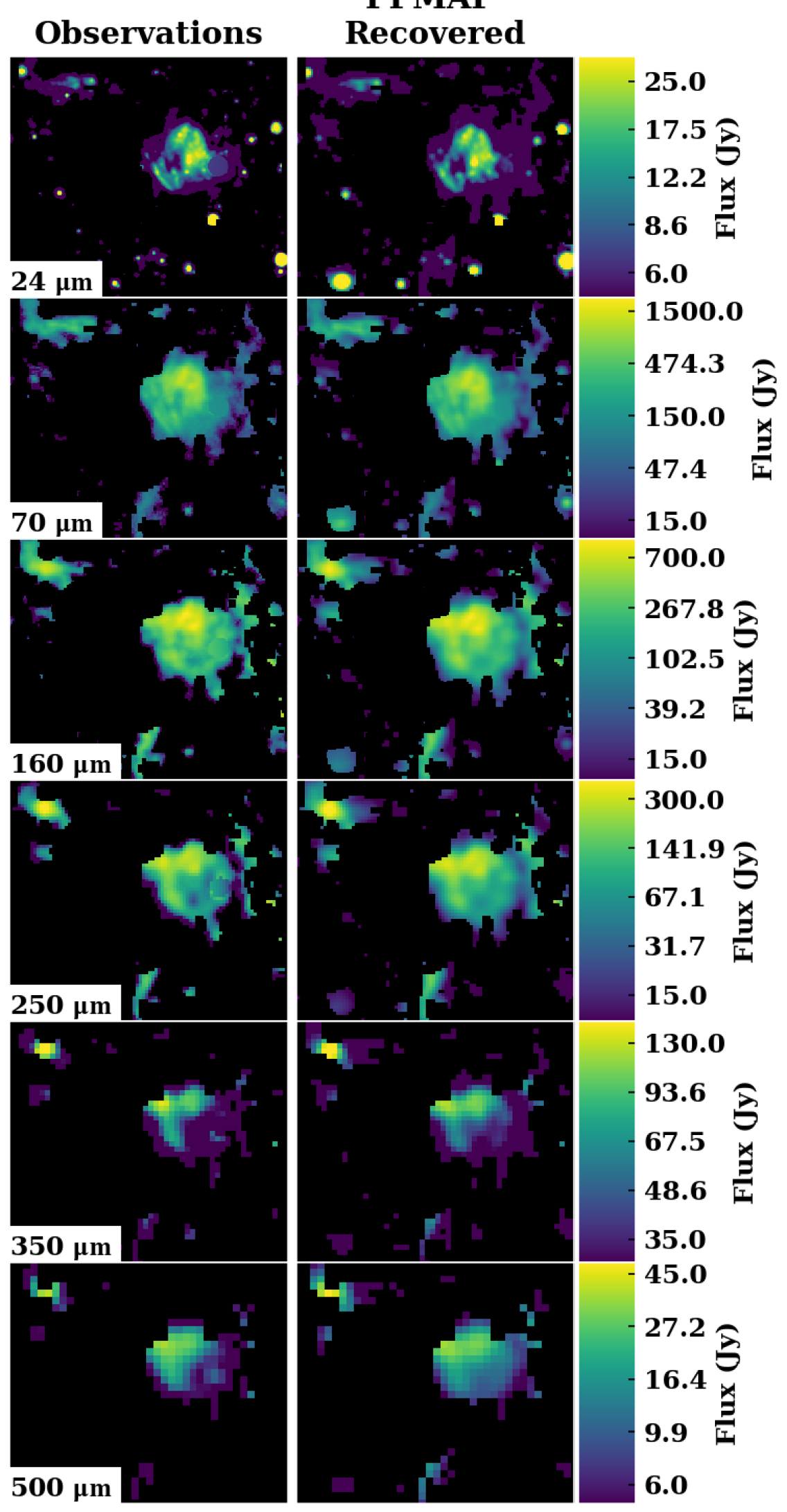
Figure 11: A grid comparing the original Spitzer and Herschel observations of the Tornado (left) with the synthetic observations (right) created by taking the results from ppmap and post-processing them.

Appendix B The X-Ray twin of the head

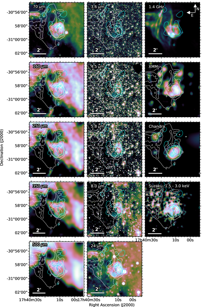
Figure 12: IR, radio, and X-ray view of the location of the Tornado head. Left column: Herschel images, middle column: Spitzer images, right top: 1.4 GHz VLA image, right second row: XMM-Newton X-ray image, right third row: Chandra X-ray image, and right bottom: Suzaku 1.5 – 4.0 keV X-ray image. We note that we have not applied a background subtraction or correction for vignetting as was done by Sawada et al. (2011). The white and cyan contours show the VLA 1.4 GHz and XMM-Newton emission respectively. There is a clear detection of emission from the head at the Spitzer and Herschel wavebands, between 5.8 and 250 µm, at 3.6, 350, and 500 µm there is emission which seems associated although it is more confused. There is a clear detection in all of the radio and X-ray images. (We use the cubehelix colour scheme, Green (2011).)

References

- Abreu-Vicente et al. (2016) Abreu-Vicente J., Ragan S., Kainulainen J., Henning T., Beuther H., Johnston K., 2016, A&A, 590, A131
- Anderson et al. (2017) Anderson L. D., et al., 2017, A&A, 605
- Angelini & White (2003) Angelini L., White N. E., 2003, The Astrophysical Journal, 586, L71
- Arendt (1989) Arendt R. G., 1989, ApJS, 70, 181
- Barlow et al. (2010) Barlow M. J., et al., 2010, A&A, 518, L138
- Becker & Helfand (1985a) Becker R. H., Helfand D. J., 1985a, Nature (ISSN 0028-0836), 313, 115
- Becker & Helfand (1985b) Becker R. H., Helfand D. J., 1985b, Nature, 313, 115
- Begelman et al. (1980) Begelman M. C., Sarazin C. L., Hatchett S. P., McKee C. F., Arons J., 1980, ApJ, 238, 722
- Bernard et al. (2010) Bernard J. P., et al., 2010, A&A, 518, L88
- Brighenti & D’Ercole (1994) Brighenti F., D’Ercole A., 1994, MNRAS, 270, 65
- Brinkmann et al. (1996) Brinkmann W., Aschenbach B., Kawai N., 1996, A&A, 312, 306
- Broadbent et al. (1989) Broadbent A., Haslam C., Osborne J. L., 1989, MNRAS, 237, 381
- Brogan & Goss (2003) Brogan C., Goss W., 2003, AJ, pp 272–276
- Burton et al. (2004) Burton M. G., Lazendic J. S., Yusef-Zadeh F., Wardle M., 2004, MNRAS, 348, 638
- Caswell et al. (1989) Caswell J. L., Kesteven M. J., Bedding T. R., Turtle A. J., 1989, PASA, 8, 184
- Chawner et al. (2019) Chawner H., et al., 2019, MNRAS, 483, 70
- Chawner et al. (2020) Chawner H., et al., 2020, MNRAS, 493, 2706
- Cox et al. (2012) Cox N. L. J., et al., 2012, A&A, 537, A35
- De Looze et al. (2017) De Looze I., et al., 2017, MNRAS, 465, 3309
- De Looze et al. (2019) De Looze I., et al., 2019, MNRAS, 488, 164
- Derlopa et al. (2020) Derlopa S., Boumis P., Chiotellis A., Steffen W., Akras S., 2020, MNRAS
- Dorschner et al. (1995) Dorschner J., Begemann B., Henning T., Jager C., Mutschke H., 1995, A&A, 300, 503
- Dubner et al. (1998) Dubner G. M., Holdaway M., Goss W. M., Mirabel I. F., 1998, AJ, 116, 1842
- Dunne et al. (2003) Dunne L., Eales S., Ivison R., Morgan H., Edmunds M., 2003, Nature, 424, 285
- Dwek et al. (1996) Dwek E., Foster S. M., Vancura O., 1996, ApJ, 457, 244
- Frail et al. (1996) Frail D. A., Reynoso E., Giacani E., Green A., Otrupcek R., 1996, AJ, 111, 1651
- Furst et al. (1987) Furst E., Reich W., Sofue Y., 1987, A&A SS, 71, 63
- Gaensler et al. (2003) Gaensler B. M., Fogel J. K. J., Slane P. O., Miller J. M., Wijnands R., Eikenberry S. S., Lewin W. H. G., 2003, ApJ, 594, L35
- Gomez et al. (2012) Gomez H. L., et al., 2012, ApJ, 760, 96
- Goodall et al. (2011) Goodall P. T., Alouani-Bibi F., Blundell K. M., 2011, MNRAS, 414, 2838
- Green (2004) Green D. A., 2004, BASI, 32, 335
- Green (2011) Green D. A., 2011, Bulletin of the Astronomical Society of India, 39, 289
- Haslam & Osborne (1987) Haslam C. G., Osborne J. L., 1987, Nature, 327, 211
- Helfand & Becker (1985) Helfand D. J., Becker R. H., 1985, in Kafatos M. C., Henry R. B. C., eds, The Crab Nebula and Related Supernova Remnants. pp 241–244
- Hewitt et al. (2008) Hewitt J. W., Yusef-Zadeh F., Wardle M., 2008, ApJ, 683, 189
- Indebetouw et al. (2014) Indebetouw R., et al., 2014, ApJ Letters, 782, L2
- James et al. (2002) James A., Dunne L., Eales S., Edmunds M. G., 2002, MNRAS, 335, 753
- Koo et al. (2016) Koo B.-C., Lee J.-J., Jeong I.-G., Seok J. Y., Kim H.-J., 2016, ApJ, 821, 20
- Law et al. (2008) Law C. J., Yusef-Zadeh F., Cotton W. D., Maddalena R. J., 2008, ApJS, 177, 255
- Lazendic et al. (2004) Lazendic J. S., Wardle M., Burton M. G., Yusef-Zadeh F., Green A. J., Whiteoak J. B., 2004, MNRAS, 354, 393
- Lombardi et al. (2014) Lombardi M., Bouy H., Alves J., Lada C. J., 2014, A&A, 566, A45
- Marsh et al. (2015) Marsh K. A., Whitworth A. P., Lomax O., 2015, MNRAS, 454, 4282
- Marsh et al. (2017) Marsh K. A., et al., 2017, MNRAS, 471, 2730
- Martin et al. (2007) Martin D. C., et al., 2007, Nature, 448, 780
- Mathis et al. (1977) Mathis J. S., Rumpl W., Nordsieck K. H., 1977, ApJ, 217, 425
- Mathis et al. (1983) Mathis J. S., Mezger P. G., Panagia N., 1983, A&A, 128, 212
- Matsuura et al. (2011) Matsuura M., et al., 2011, Science, 333, 1258
- Meynet & Maeder (2003) Meynet G., Maeder A., 2003, A&A, 404, 975
- Meynet & Maeder (2005) Meynet G., Maeder A., 2005, A&A, 429, 581
- Milne (1979) Milne D. K., 1979, Australian Journal of Physics, 32, 83
- Molinari et al. (2010) Molinari S., et al., 2010, PASP, 122, 314
- Molinari et al. (2016) Molinari S., et al., 2016, A&A, 591
- Noriega-Crespo et al. (1997) Noriega-Crespo A., van Buren D., Cao Y., Dgani R., 1997, AJ, 114, 837
- Paredes et al. (2000) Paredes J. M., Marti J., Ribó M., Massi M., 2000, Science, 288, 2340
- Pilbratt et al. (2010) Pilbratt G. L., et al., 2010, A&A, 518, L1
- Pinheiro Goncalves et al. (2011) Pinheiro Goncalves D., et al., 2011, AJ, 142, 42
- Planck Collaboration (2016) Planck Collaboration 2016, A&A, 596, A109
- Planck Collaboration XXXI (2016) Planck Collaboration XXXI 2016, A&A, 586, A134
- Priestley et al. (2019) Priestley F. D., Barlow M. J., De Looze I., 2019, MNRAS, 485, 440
- Priestley et al. (2020) Priestley F. D., Barlow M. J., De Looze I., Chawner H., 2020, MNRAS, 491, 6020
- Rho & Petre (1998) Rho J., Petre R., 1998, ApJ, 503, L167
- Rho et al. (2008) Rho J., et al., 2008, ApJ, 673, 271
- Rho et al. (2018) Rho J., et al., 2018, MNRAS, 479, 5101
- Safi-Harb & Ögelman (1997) Safi-Harb S., Ögelman H., 1997, ApJ, 483, 868
- Sawada et al. (2011) Sawada M., Tsuru T. G., Koyama K., Oka T., 2011, PASJ, 63, S849
- Shaver et al. (1985) Shaver P. A., Salter C. J., Patnaik A., van Gorkom J. H., Hunt G. C., 1985, Nature, 313, 113
- Shull et al. (1989) Shull J. M., Fesen R. A., Saken J. M., 1989, Astrophysical Journal, 346, 860
- Stewart et al. (1994) Stewart R. T., Haynes R. F., Gray A. D., Reich W., 1994, ApJ, 432, L39
- Temim et al. (2012) Temim T., Sonneborn G., Dwek E., Arendt R. G., Gehrz R. D., Slane P., Roellig T. L., 2012, ApJ, 753, 72
- Temim et al. (2017) Temim T., Dwek E., Arendt R. G., Borkowski K. J., Reynolds S. P., Slane P., Gelfand J. D., Raymond J. C., 2017, ApJ, 836, 129
- The Astropy Collaboration et al. (2013) The Astropy Collaboration et al., 2013, A&A, 558, A33
- The Astropy Collaboration et al. (2018) The Astropy Collaboration et al., 2018, AJ, 156
- Ueta et al. (2008) Ueta T., et al., 2008, PASJ, 60, 407
- Werner et al. (2004) Werner M. W., et al., 2004, ApJSS, 154, 1
- Whiteoak & Green (1996) Whiteoak J. B., Green A. J., 1996, A&A SS, 118, 329
- Williams et al. (2006) Williams B. J., et al., 2006, ApJ, 652, L33
- Winkler & Clark (1974) Winkler P. F. J., Clark G. W., 1974, ApJ, 191, L67
- Yusef-Zadeh et al. (2003) Yusef-Zadeh F., Wardle M., Rho J., Sakano M., 2003, ApJ, 585, 319
- Zubko et al. (1996) Zubko V. G., Mennella V., Colangeli L., Bussoletti E., 1996, MNRAS, 282, 1321