Perturbative tomography of small errors in quantum gates

Abstract

We propose an efficient protocol to fully reconstruct a set of high-fidelity quantum gates. Usually, the efficiency of reconstructing high-fidelity quantum gates is limited by the sampling noise. Our protocol is based on a perturbative approach and has two stages. In the first stage, the unital part of noisy quantum gates is reconstructed by measuring traces of maps, and the trace can be measured by amplifying the noise in a way similar to randomised benchmarking and quantum spectral tomography. In the second stage, by amplifying the non-unital part using the unital part, we can efficiently reconstruct the non-unital part. We show that the number of measurements needed in our protocol scales logarithmically with the error rate of gates.

I Introduction

Quantum computing can solve many problems that are intractable for classical computing. In the standard circuit model of universal quantum computing, all quantum algorithms can be realised by combining elementary unitary evolutions, i.e. quantum gates Nielsen and Chuang (2002). In the past twenty years, the fidelity of quantum gates have been constantly improved. In superconducting and trapped-ion systems, single-qubit gate fidelities have achieved 99.9% Barends et al. (2014) and 99.9999% Harty et al. (2014), respectively. However, these fidelities are not sufficiently low for directly implementing large-scale quantum algorithms, e.g. Shor’s algorithm Beauregard (2002). Methods such as the quantum error correction Steane (1996); Calderbank et al. (1997); Fowler et al. (2012); O’Gorman and Campbell (2017); Chiaverini et al. (2004); Reed et al. (2012) and mitigation protocols Li and Benjamin (2017); Temme et al. (2017); Endo et al. (2018) have been proposed and demonstrated Kandala et al. (2019); Song et al. (2019); Zhang et al. (2020) to minimise the impact of errors in the quantum computing. Quantum gate characterisation is of importance to debug the gates and take the full advantage of these error correction methods. The common approaches of gate characterisation include measuring the average fidelity through randomized benchmarking Emerson et al. (2005); Knill et al. (2008); Magesan et al. (2011, 2012); Sheldon et al. (2016); Fong and Merkel (2017); Proctor et al. (2017); Wallman (2018); Onorati et al. (2019); Lu et al. (2015); McKay et al. (2019) and reconstructing all the detailed information using quantum tomography Chuang and Nielsen (1997); Poyatos et al. (1997); D’Ariano and Presti (2001); Altepeter et al. (2003); Mohseni and Lidar (2006); Merkel et al. (2013); Blume-Kohout et al. (2013); Stark (2014); Greenbaum (2015); Blume-Kohout et al. (2017); Sugiyama et al. (2018). Quantum spectral tomography is recently proposed to obtain eigenvalues of quantum gates Helsen et al. (2019).

In this paper, we describe a method of characterising noisy gates that are closed to perfect unitary gates. The unital part of the completely positive map describing a noisy gate can be reconstructed by measuring the traces of maps, e.g. using randomised benchmarking Kimmel et al. (2014). We propose a way to measure the trace using deterministic gate sequences inspired by the quantum spectral tomography Helsen et al. (2019). In the trace measurement, the fidelity decreases slower with the sequence length in deterministic gate sequences compared with random sequences. Therefore, we can use sufficiently long sequences to amplify the error for the efficient measurement Blume-Kohout et al. (2017). The reconstruction of the unital part is based on a perturbative approach, we express the error in a gate as a perturbation and neglecting high-order effects of the error in the data analysis. With the unital part reconstructed, we can amplify and efficiently measure the non-unital part in a similar way.

The obstacle of high-fidelity-gate reconstruction is the sampling noise. In order to reconstruct a noisy gate, we need to suppress the sampling noise to a level that is lower than the error rate. Our method inherits the advantage of randomized benchmarking and quantum spectral tomography, that the error is amplified in a long gate sequence to reduce the sampling noise Blume-Kohout et al. (2017). In our protocol, the problem of state preparation and measurement errors is overcome as the same as in the quantum gate set tomography (GST) Merkel et al. (2013); Blume-Kohout et al. (2013); Stark (2014); Greenbaum (2015); Blume-Kohout et al. (2017); Sugiyama et al. (2018). We focus on the case of one-qubit gates in this paper, and the method can be generalised to multi-qubit gates. The correlated errors in multi-qubit systems can be characterised using the perturbative tomography protocol proposed recently Govia et al. (2020). We find that the number of measurements needed for sufficiently low sampling noise scales logarithmically with the error rate of gates. Therefore, this work paves an efficient way for the quantum tomography of high-fidelity gates.

This paper is organized as follows. In Sec. II we give a brief review on completely positive maps, including the Pauli transfer matrix representation of maps Greenbaum (2015). In Sec. III, we discuss the error accumulation in a deterministic gate sequence. In Sec. IV, we present the method for trace measurement, and reconstructions of unital and non-unital parts. In Sec. V, we numerically demonstrate our protocol with the finite sampling noise. Conclusions are given in In Sec. VI.

II Quantum maps

The completely positive map describes the evolution of a quantum system without initial correlation between the system and environment Choi (1975); Jordan et al. (2004), which can be written in the operator-summation form Nielsen and Chuang (2002):

$$\mathcal{M}(\rho)=\sum_{q}K_{q}\rho K_{q}^{\dagger}.$$ (1)

The Kraus operators satisfy $\sum_{q}K_{q}^{\dagger}K_{q}=\openone$ if the map is trace-preserving, where $\openone$ is the identity operator. The Pauli transfer matrix of a map reads

$$M_{\sigma,\tau}=d^{-1}\mathrm{Tr}\left[\sigma\mathcal{M}(\tau)\right],$$ (2)

which is the matrix representation of the map using Pauli operators as the basis of the operator space, according to the Hilbert-Schmidt inner product. Here, $\sigma$ and $\tau$ are Pauli operators, and $d$ is the dimension of the Hilbert space. We can find that all elements of the Pauli transfer matrix are real, and $M_{\sigma,\tau}\in[-1,1]$. Let $M_{j}$ be the Pauli transfer matrix of the map $\mathcal{M}_{j}$, then the matrix of $\mathcal{M}_{i}\mathcal{M}_{j}$ is $M_{i}M_{j}$.

We always take the identity operator as the first element in Pauli operators. The first row of the matrix is $M_{\openone,\sigma}=\delta_{\openone,\sigma}$ for a trace-preserving map. Therefore, we can write the matrix of a trace-preserving map in the form

$$M=\left[\begin{array}[]{cc}1&\vec{0}^{\rm\,T}\\ \vec{k}&E\end{array}\right]$$ (5)

The matrix is $d^{2}$-dimensional in general. In this paper, we only consider the case of one qubit, i.e. $d=2$. Then, $\vec{0}$ and $\vec{k}$ are three-dimensional column vectors, all elements of $\vec{0}$ are zero, and $E$ is a three-dimensional matrix. If the map is unital, $\vec{k}=\vec{0}$. We call $E$ the unital part and $\vec{k}$ the non-unital part. When the map is completely positive, there is a constraint on $E$ and $\vec{k}$, which is Rudnicki et al. (2018)

$$\|\vec{k}\|^{2}\leq 1-|\lambda_{1}|^{2}-|\lambda_{2}|^{2}-|\lambda_{3}|^{2}+2\lambda_{1}\lambda_{2}\lambda_{3},$$ (6)

where $\lambda_{l}$ are eigenvalues of $E$.

An ideal quantum gate is a unitary evolution in the form $\mathcal{M}^{\rm i}(\rho)=U\rho U^{\dagger}$, where $U$ is the unitary operator. We use $M^{\rm i}$ to denote the Pauli transfer matrix of the ideal gate $\mathcal{M}^{\rm i}$, which is always a unitary matrix. Let $E^{\rm i}$ and $\vec{k}^{\rm i}$ be the unital and non-unital parts of $M^{\rm i}$, then $E^{\rm i}$ is a unitary matrix, all eigenvalues of $E^{\rm i}$, i.e. $\lambda^{\rm i}_{l}$, have the same absolute value of $1$, and $\vec{k}^{\rm i}=\vec{0}$. Accordingly, for a quantum gate with high-fidelity, absolute values $|\lambda_{l}|$ are all close to $1$, and the non-unital part $\vec{k}$ is close to zero.

The error in a quantum gate is the difference between the actual noisy gate and the ideal gate, i.e.

$$\delta M=M-M^{\rm i}.$$ (7)

When the gate fidelity is high, $\delta M$ must be close to zero.

In this paper, we will consider a set of quantum gates. We use the subscript to label the gate, i.e. $M_{j}$, $M_{j}^{\rm i}$ and $\delta M_{j}$ are respectively the actual noisy matrix, ideal matrix and error of the gate-$j$. The error can be gate dependent. We assume that the error is time-independent and uncorrelated Huo and Li (2018).

III Error accumulation

To efficiently measure the small error in a quantum gate, we can repeat the noisy gate such that the error accumulates with the repetition length. If the gate $\mathcal{M}$ is repeated for $n$ times, the corresponding Pauli transfer matrix reads

$$M^{n}=\left[\begin{array}[]{cc}1&\vec{0}^{\rm\,T}\\ (\sum_{q=0}^{n-1}E^{q})\vec{k}&E^{n}\end{array}\right].$$ (10)

The magnitude of the unital part decreases exponentially with the repetition length $n$, i.e. $E^{n}\sim\lambda_{l}^{n}$. If the gate is of high-fidelity, the eigenvalue $|\lambda_{l}|=1-\epsilon$ is close to $1$. Then, we can take $n\sim 1/\epsilon$ such that $E^{n}$ is significantly changed by the accumulated error. If $E^{n}$ is measured with the accuracy $\eta$, we can estimate the error in the unital part of one gate with the accuracy $\sim\eta/n$, i.e. $\sim\eta\epsilon$.

By repeating the gate, the non-unital part is amplified by $\sum_{q=0}^{n-1}E^{q}$. In three eigenvalues of $E$, one of them (the eigenvalue itself rather than the absolute value) is always close to $1$, if the fidelity is high. Without loss of generality, we assume that $\lambda_{1}=1-\epsilon^{\prime}$. Then, $\sum_{q=0}^{n-1}E^{q}\sim 1/\epsilon^{\prime}$ in the limit $n\rightarrow\infty$. If the non-unital part of $M^{n}$ is measured with the accuracy $\eta^{\prime}$, we can estimate the error in the non-unital part of one gate with the accuracy $\sim\eta^{\prime}\epsilon^{\prime}$.

Later, we will show how to reconstruct a noisy gate efficiently by accumulating the error. We will find that in the repeated gate, the trace of map is the robust information that can be extracted with high accuracy, and the estimation of individual eigenvalues is not robust. In the randomised benchmarking, the trace of the product of the noisy gate and an ideal Clifford gate can be measured, in which the trace is related to the relative fidelity between the noisy gate and the ideal Clifford gate Kimmel et al. (2014). The repetition length is limited by the relative fidelity in the randomised benchmarking. To reconstruct the noisy gate, we need to measure traces of a set of products, and it is impossible that relative fidelities are high for all of them. In our case, the repetition length is limited by the eigenvalues. As long as the gate is close to a unitary gate, the absolute values of eigenvalues are close to $1$, and a large repetition length is permitted.

IV Protocol

The protocol has two stages. In the first stage, the unital part of gates is reconstructed by using trace measurements. In the second stage, the non-unital part is reconstructed by amplifying them using the unital part. We present our protocol as follows.

IV.1 Trace measurement

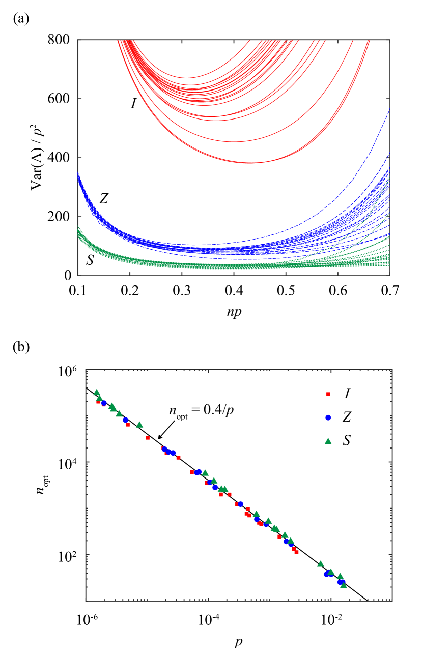
Figure 1: (a) The variance as a function of $n$. (b) The optimal value of $n$ (i.e. $n_{\rm opt}$) that minimizes the variance in (a). Each curve in (a) corresponds to a gate with randomly generated error (see Appendix A). The error rate $p$ is randomly selected in the range $\sim 10^{-2}-10^{-6}$.

In the experiment, it is difficult to observe the effect of low-level noise such as in high-fidelity gates. To characterise the noise, we can repeat the noisy gate to accumulate the errors, similar to the randomised benchmarking Knill et al. (2008); Magesan et al. (2011, 2012); Sheldon et al. (2016); Fong and Merkel (2017); Onorati et al. (2019); Wallman (2018); Proctor et al. (2017) and quantum spectral tomography Helsen et al. (2019). The matrix of the repeated gate is $M^{n}$, see Eq. (10). The eigenvalues of $M^{n}$ are $1$, $\lambda_{1}^{n}$ ,$\lambda_{2}^{n}$ and $\lambda_{3}^{n}$, where $\lambda_{1}$, $\lambda_{2}$ and $\lambda_{3}$ are eigenvalues of $E$. We note that $M$ and $M^{n}$ can always be expressed in the Jordan normal form, which leads to the formula

$$\mathrm{Tr}(M^{n})=1+\lambda_{1}^{n}+\lambda_{2}^{n}+\lambda_{3}^{n}$$ (11)

The protocol for measuring the trace is as follows:

• Use GST to obtain an estimate of $M^{l}$, and the estimate is $\hat{M}_{l}$, where $l=n,2n,3n$; compute the trace of the unital part $t_{l}=\mathrm{Tr}(\hat{M}_{l})-1$ for each $l$;

• Solve the system of equations(SOE) to obtain $\lambda_{1}$, $\lambda_{2}$ and $\lambda_{3}$; compute $\Lambda=1+\lambda_{1}+\lambda_{2}+\lambda_{3}$, which is the estimate of the trace of the map $\mathrm{Tr}(M)$.

  $$\lambda_{1}^{n}+\lambda_{2}^{n}+\lambda_{3}^{n} =t_{n},$$ (12a)

  $$\lambda_{1}^{2n}+\lambda_{2}^{2n}+\lambda_{3}^{2n} =t_{2n},$$ (12b)

  $$\lambda_{1}^{3n}+\lambda_{2}^{3n}+\lambda_{3}^{3n} =t_{3n}$$ (12c)

In GST, because of the state preparation and measurement errors, the estimate and the actual matrix are related by an unknown similarity transformation, i.e. $M^{l}=T\hat{M}_{l}T^{-1}$, assuming the sampling error in GST is negligible Merkel et al. (2013); Greenbaum (2015); Blume-Kohout et al. (2017); Rudnicki et al. (2018); Stark (2014); Sugiyama et al. (2018); Blume-Kohout et al. (2013). Although the transformation is unknown, the trace can be directly obtained using the estimate, i.e. $\mathrm{Tr}(M^{l})=\mathrm{Tr}(T\hat{M}_{l}T^{-1})=\mathrm{Tr}(\hat{M}_{l})$, i.e. the trace measurement is robust to the state preparation and measurement errors.

In our protocol, the eigenvalues are computed by solving SOE. Note that there are multiple solutions of SOE (12). These solutions are close to each other when $n$ is large, and the difference between them is typically $O(2\pi/n)$. However, only one of them is correct. In order to efficiently identify the correct solution, we can implement the trace measurement (to compute eigenvalues) for a monotonically increasing series of $n$, i.e. $n=n_{1},n_{2},n_{3},\ldots,n_{\rm max}$. For each value of $n$, we construct and solve SOE as in the protocol. We always take $n_{1}=1$ such that solutions of $n=n_{1}$ are significantly different. Then, under the assumption that the error is small, we can rule out solutions that are far from eigenvalues of $M^{\rm i}$. For $n=n_{i>1}$, we choose the solution that is the closest to the solution of $n=n_{i-1}$. In this way, we only need to reduce the sampling noise at $n=n_{i-1}$ to the level that the confidence interval is sufficiently small for distinguishing solutions of $n=n_{i}$. In the numerical demonstrations, we will show that such a procedure is efficient by taking a power series of $n$.

$U_{1}=e^{\frac{i\pi}{6}\hat{Z}}$	$U_{2}=e^{{\frac{-i\pi}{3}}\frac{\hat{X}+\hat{Y}-\hat{Z}}{\sqrt{3}}}$
$U_{3}=e^{{\frac{-2i\pi}{3}}\frac{\hat{X}+\hat{Y}-\hat{Z}}{\sqrt{3}}}$	$U_{4}=e^{{\frac{-i\pi}{3}}\frac{\hat{X}+\hat{Y}+\hat{Z}}{\sqrt{3}}}$
$U_{5}=e^{{\frac{-2i\pi}{3}}\frac{\hat{X}+\hat{Y}+\hat{Z}}{\sqrt{3}}}$	$U_{6}=e^{{\frac{-i\pi}{3}}\frac{\hat{X}-\hat{Y}+\hat{Z}}{\sqrt{3}}}$
$U_{7}=e^{{\frac{-2i\pi}{3}}\frac{\hat{X}-\hat{Y}+\hat{Z}}{\sqrt{3}}}$

Table 1: The gate set used in the numerical demonstration. The ideal map of the gate $U_{i}$ is $\mathcal{M}_{i}^{\rm i}(\rho)=U_{i}\rho U_{i}^{\dagger}$.

Finally, the trace is computed using eigenvalues obtained at $n=n_{\rm max}$. We need to choose a sufficiently large $n_{\rm max}$ in order to amplify the noise. Later we show that the optimal value of $n_{\rm max}$ is $\sim 0.4/p$. Here, $p=1-F$ is the error rate, and $F$ is the average fidelity Nielsen and Chuang (2002). We remark that we can also use the method of least squares Wolberg (2006) and the matrix pencil method Sarkar and Pereira (1995) to work out the eigenvalues and then compute the trace.

Variance of the trace measurement

The variance of $\Lambda(t_{n},t_{2n},t_{3n})$ is

$${\rm Var}(\Lambda)\approx\sum_{l=n,2n,3n}\left(\frac{\partial\Lambda}{\partial t_{l}}\right)^{2}{\rm Var}[t_{l}]$$ (13)

where

$$\frac{\partial\Lambda}{\partial t_{n}} =\frac{\lambda_{1}^{-n}\lambda_{2}^{-n}\lambda_{3}^{-n}(\lambda_{1}\lambda_{2}^{2n}\lambda_{3}^{2n}(\lambda_{2}^{n}-\lambda_{3}^{n})+\lambda_{1}^{3n}(\lambda_{2}^{2n}\lambda_{3}-\lambda_{2}\lambda_{3}^{2n})+\lambda_{1}^{2n}(-\lambda_{2}^{3n}\lambda_{3}+\lambda_{2}\lambda_{3}^{3n}))}{(\lambda_{1}^{n}-\lambda_{2}^{n})(\lambda_{1}^{n}-\lambda_{3}^{n})(\lambda_{2}^{n}-\lambda_{3}^{n})n}$$ (14a)

$$\frac{\partial\Lambda}{\partial t_{2n}} =\frac{\lambda_{1}^{-n}\lambda_{2}^{-n}\lambda_{3}^{-n}(\lambda_{1}^{3n}(-\lambda_{2}^{n}\lambda_{3}+\lambda_{2}\lambda_{3}^{n})+\lambda_{1}^{n}(\lambda_{2}^{3n}\lambda_{3}-\lambda_{2}\lambda_{3}^{3n})+\lambda_{1}(-\lambda_{2}^{3n}\lambda_{3}^{n}+\lambda_{2}^{n}\lambda_{3}^{3n}))}{2(\lambda_{1}^{n}-\lambda_{2}^{n})(\lambda_{1}^{n}-\lambda_{3}^{n})(\lambda_{2}^{n}-\lambda_{3}^{n})n}$$ (14b)

$$\frac{\partial\Lambda}{\partial t_{3n}} =\frac{\lambda_{1}^{-n}\lambda_{2}^{-n}\lambda_{3}^{-n}(\lambda_{1}\lambda_{2}^{n}\lambda_{3}^{n}(\lambda_{2}^{n}-\lambda_{3}^{n})+\lambda_{1}^{2n}(\lambda_{2}^{n}\lambda_{3}-\lambda_{2}\lambda_{3}^{n})+\lambda_{1}^{n}(-\lambda_{2}^{2n}\lambda_{3}+\lambda_{2}\lambda_{3}^{2n}))}{3(\lambda_{1}^{n}-\lambda_{2}^{n})(\lambda_{1}^{n}-\lambda_{3}^{n})(\lambda_{2}^{n}-\lambda_{3}^{n})n}$$ (14c)

When $\lambda_{1}\neq\lambda_{2}=\lambda_{3}$, we have

$$\lim_{\lambda_{2}\to\lambda_{3}}\frac{\partial\Lambda}{\partial t_{n}} =\frac{\lambda_{1}^{-n}\lambda_{3}^{-n}(\lambda_{1}^{2n}\lambda_{3}^{1+n}(1-3n)+\lambda_{1}\lambda_{3}^{3n}n+\lambda_{1}^{3n}\lambda_{3}(-1+2n))}{(\lambda_{1}^{n}-\lambda_{3}^{n})^{2}n^{2}}$$ (15a)

$$\lim_{\lambda_{2}\to\lambda_{3}}\frac{\partial\Lambda}{\partial t_{2n}} =\frac{\lambda_{1}^{-n}\lambda_{3}^{-2n}(-\lambda_{1}^{3n}\lambda_{3}(-1+n)+\lambda_{1}^{n}\lambda_{3}^{1+2n}(-1+3n)-2\lambda_{1}\lambda_{3}^{3n}n)}{2(\lambda_{1}^{n}-\lambda_{3}^{n})^{2}n^{2}}$$ (15b)

$$\lim_{\lambda_{2}\to\lambda_{3}}\frac{\partial\Lambda}{\partial t_{3n}} =\frac{\lambda_{1}^{-n}\lambda_{3}^{-2n}(\lambda_{1}^{n}\lambda_{3}^{1+n}(1-2n)+\lambda_{1}^{2n}\lambda_{3}(-1+n)+\lambda_{1}\lambda_{3}^{2n}n)}{3(\lambda_{1}^{n}-\lambda_{3}^{n})^{2}n^{2}}$$ (15c)

When $\lambda_{1}=\lambda_{2}=\lambda_{3}$, we have

$$\lim_{\lambda_{2},\lambda_{3}\to\lambda_{1}}\frac{\partial\Lambda}{\partial t_{n}} =\frac{\lambda_{1}^{1-n}(1-5n+6n^{2})}{2n^{3}}$$ (16a)

$$\lim_{\lambda_{2},\lambda_{3}\to\lambda_{1}}\frac{\partial\Lambda}{\partial t_{2n}} =\frac{\lambda_{1}^{1-2n}(1-4n+3n^{2})}{2n^{3}}$$ (16b)

$$\lim_{\lambda_{2},\lambda_{3}\to\lambda_{1}}\frac{\partial\Lambda}{\partial t_{3n}} =\frac{\lambda_{1}^{1-3n}(-1+n)(-1+2n)}{6n^{3}}$$ (16c)

Therefore, the variance is always convergent even if eigenvalues are degenerate. We remark that in the case $\lambda_{1}\neq\lambda_{2}=\lambda_{3}$, we need to avoid the value of $n$ with $\lambda_{1}^{n}\approx\lambda_{3}^{n}$.

The variance is plotted in Fig. 1 for quantum gates with randomly generated errors. The identity gate $I$, Pauli gate $Z$ and phase gate $S$ are considered, corresponding to the cases $\lambda_{1}=\lambda_{2}=\lambda_{3}$, $\lambda_{1}\neq\lambda_{2}=\lambda_{3}$ and $\lambda_{1}\neq\lambda_{2}\neq\lambda_{3}$, respectively. For each ideal gate, twenty noisy gates are generated by computing the time integral of randomly generated Lindblad superoperator (see Appendix A). We take $n=4l+1$, where $l$ is an integer, such that ${\lambda_{1}}^{n}\neq{\lambda_{3}}^{n}$ for the gate $S$. We can find that the variance is minimised around $n\sim 0.4/p$. The gate $I$ has the highest variance, and the gate $S$ has the lowest variance in the three gates.

IV.2 Unital part reconstruction

In our protocol, we reconstruct the unital part by measuring the trace of actual noisy gates using the method given in Sec. IV.1. According to Ref. Kimmel et al. (2014), we can also reconstruct the unital part of the map $M$ by measuring the trace $\mathrm{Tr}(C^{\rm i}M)$, where $C^{\rm i}$ is one of ideal Clifford gates, and the trace can be measured using the randomised benchmarking.

We use the perturbative approach. For the gate-$j$, we express the Pauli transfer matrix of the actual noisy gate as $M_{j}=M_{j}^{\rm i}+\delta M_{j}$. Because our aim is to reconstruct the map rather than measuring the relative fidelity with respect to an ideal gate, $M_{j}^{\rm i}$ is up to choice, however, must be close to the actual noisy gate $M_{j}$. The error can be written as

$$\delta M_{j}=\left[\begin{array}[]{cc}0&\vec{0}^{\rm\,T}\\ \delta\vec{k}_{j}&\delta E_{j}\end{array}\right].$$ (19)

In this section, we show how to reconstruct $\delta E_{j}$.

For a quadruple map $\mathcal{M}_{i,j,k,l}=\mathcal{M}_{i}\mathcal{M}_{j}\mathcal{M}_{k}\mathcal{M}_{l}$, the Pauli transfer matrix is

$$M_{i,j,k,l}=M_{i}M_{j}M_{k}M_{l}$$ (20)

$$= M_{i}^{\rm i}M_{j}^{\rm i}M_{k}^{\rm i}M_{l}^{\rm i}+\delta M_{i}M_{j}^{\rm i}M_{k}^{\rm i}M_{l}^{\rm i}+M_{i}^{\rm i}\delta M_{j}M_{k}^{\rm i}M_{l}^{\rm i}$$

$$+M_{i}^{\rm i}M_{j}^{\rm i}\delta M_{k}M_{l}^{\rm i}+M_{i}^{\rm i}M_{j}^{\rm i}M_{k}^{\rm i}\delta M_{l}+O(\delta^{2}).$$

By measuring the trace of quadruple maps, we are able to obtain the unital part of each $\delta M_{j}$. We remark that $\mathrm{Tr}(M_{i}^{\rm i}M_{j}^{\rm i}M_{k}^{\rm i}\delta M_{l})=\mathrm{Tr}(E_{i}^{\rm i}E_{j}^{\rm i}E_{k}^{\rm i}\delta E_{l})$.

The protocol for reconstructing the unital part is as follows:

• Given a set of gates $\{M_{j}\}$, measure the trace of quadruple maps $\mathrm{Tr}(M_{i,j,k,l})$ using our protocol;

• Solve the SOE for a set of quadruple maps,

  $$\mathrm{Tr}(M_{i,j,k,l}) = \mathrm{Tr}(M_{i}^{\rm i}M_{j}^{\rm i}M_{k}^{\rm i}M_{l}^{\rm i})+\mathrm{Tr}(E_{j}^{\rm i}E_{k}^{\rm i}E_{l}^{\rm i}\delta E_{i})$$ (21)

  $$+\mathrm{Tr}(E_{k}^{\rm i}E_{l}^{\rm i}E_{i}^{\rm i}\delta E_{j})+\mathrm{Tr}(E_{l}^{\rm i}E_{i}^{\rm i}E_{j}^{\rm i}\delta E_{k})$$

  $$+\mathrm{Tr}(E_{i}^{\rm i}E_{j}^{\rm i}E_{k}^{\rm i}\delta E_{l})$$

  to obtain each element of $\delta E_{j}$;

• Iterate the second step by replacing $M_{j}^{\rm i}$ with $M_{j}^{\rm i}+\delta E_{j}$.

The iteration can rapidly increase the accuracy by taking into account higher-order effects, which is not necessary when $\delta E_{j}$ is sufficiently small. In our numerical simulation that we will show later, the iteration is not used.

5,2,3,6	7,2,2,6	5,1,4,3	6,3,4,1	6,1,4,6	1,5,3,5	6,1,2,5	5,5,2,6
4,2,1,4	3,2,3,4	4,7,2,7	2,1,2,3	1,7,1,2	7,3,6,3	7,4,1,7	5,6,4,6
3,1,3,3	5,1,5,1	1,2,4,3	3,6,1,4	4,5,4,4	5,4,5,1	5,3,5,5	5,7,1,4
4,1,4,6	2,2,2,2	7,1,2,3	1,4,7,6	1,1,5,1	6,3,6,1	5,1,3,2	6,4,4,3
3,2,6,6	2,7,4,1	7,6,5,2	6,4,1,6	6,7,1,6	5,4,2,5	1,6,4,1	1,5,6,7
2,5,2,5	1,1,5,6	7,2,6,5	5,6,5,7	1,7,6,5	5,2,3,2	2,7,6,1	7,2,1,5
1,5,1,6	1,6,7,4	7,7,2,3	6,5,4,5	4,5,2,5	5,4,7,4	1,2,2,1	6,7,1,3
7,4,7,5	7,4,2,7	5,4,1,2	2,3,3,3	1,1,3,7	1,7,6,2	7,6,4,4	5,7,4,4
4,6,3,1	1,2,5,2	6,7,1,2	1,4,7,7	5,1,7,5	1,7,5,7	2,7,1,5	5,1,1,5
2,5,4,6	7,4,6,3	1,5,6,1	2,3,6,5	5,2,5,1	7,5,3,3	5,3,7,3	4,1,1,7
4,2,1,7	7,4,3,3	5,4,1,3	2,7,1,2	1,2,3,6	5,4,1,2	1,3,7,1	6,6,2,3
5,1,4,2	1,2,2,6	4,4,4,5	1,1,6,6	1,7,7,6	4,1,2,5	2,2,2,1	4,2,7,3
4,7,5,7	4,7,3,3	2,5,3,6	4,1,4,4

Table 2: Quadruple maps for reconstructing the unital part. Here $(i,j,k,l)$ denotes the quadruple map $M_{i,j,k,l}=M_{i}M_{j}M_{k}M_{l}$.

We do not need to measure all quadruple maps. Each matrix $\delta E_{n}$ has nine elements. For a set of $N$ gates, the total number of matrix elements is $9N$. However, we can never find $9N$ linearly independent equations, because of the gauge problem of GST Greenbaum (2015); Rudnicki et al. (2018) i.e. the Pauli transfer matrix can only be reconstructed up to a similarity transformation. Therefore, the maximum number of linearly independent equations is $9N-8$, where $8$ is due to the similarity transformation of three-dimensional matrices. See Appendix B. Therefore, we need to identify and measure at least $9N-8$ quadruple maps that provide $9N-8$ linearly independent equations.

In Table 1, we list seven gates, whose quadruple maps lead to $9N-8$ linearly independent equations. A hundred quadruple maps are given in Table 2, and $9\times 7-8=55$ of them are linearly independent. We choose these quadruple maps because their unital parts have three different eigenvalues, in order to minimise the variance. In principle, we can also use the product of two and three maps rather than four to construct linear equations. However, we find numerically that they are insufficient for constructing $9N-8$ linearly independent equations if we only choose the double or triple maps with three different eigenvalues. This gate set is complete, and any unital map can be expressed as a linear combination of maps of these gates and their products.

Once we have a complete set of gates reconstructed, the unital part of any other map $M^{\prime}$ can be reconstructed by measuring $\mathrm{Tr}(M_{j}M^{\prime})$ Kimmel et al. (2014). The protocol is as follows: Given a gate $M^{\prime}$ and a set of $9$ linearly independent maps $\{M_{j}\}$ (maps of gates in the gate set and their products), measure the trace $\mathrm{Tr}(M_{j}M^{\prime})$; then solve SOE

$$\mathrm{Tr}(M_{j}M^{\prime}) = \mathrm{Tr}(E_{j}E^{\prime})+1$$ (22)

to obtain each element of $E^{\prime}$, where $E^{\prime}$ is the unital part of $M^{\prime}$.

IV.3 Non-unital part reconstruction

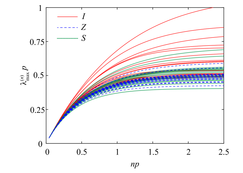
Figure 2: The largest singular value $\lambda_{\rm max}^{(n)}$ of $E^{(n)}$ as a function of number of repetitions $n$. $p$ is the error rate. Each curve corresponds to a gate with randomly generated error (see Appendix A). The error rate $p$ is randomly selected in the range $\sim 10^{-2}-10^{-6}$.

Given the unital part reconstructed, we can amplify and reconstruct the non-unital part in a similar way. Repeating the map $M$ for $n$ times, the non-unital part of $M^{n}$ is $\vec{k}^{(n)}=E^{(n)}\vec{k}$, where $E^{(n)}=\sum_{q=0}^{n-1}E^{q}$ [see Eq. (10)]. Using the the conventional quantum tomography protocol, e.g. GST, we can obtain the non-unital part of $M^{n}$ in the experiment. By solving the equation, we can compute the non-unital part of $M$, i.e. $\vec{k}={E^{(n)}}^{-1}\vec{k}^{(n)}$. We remark that the unital part $E$ has been reconstructed. Because $\vec{k}^{(n)}$ is directly measured in the experiment, it has a finite variance due to the sampling noise. Therefore, the variance of $\vec{k}$ depends on singular values of $E^{(n)}$.

When the gate error is small, the unital part $E$ is close to a unitary matrix, and at least one of its eigenvalues is close to one. Without loss of generality, we suppose $\lambda_{1}$ is the eigenvalue close to one. Then $1-\lambda_{1}\sim p$, where $p$ is the error rate. The largest singular value of $E^{(n)}$ is $\lambda_{\rm max}^{(n)}\sim\frac{1}{1-\lambda_{1}}$, when $n$ is sufficiently large. In Fig. 2, we plot the largest singular value $\lambda_{\rm max}^{(n)}$ of $E^{(n)}$ for quantum gates with randomly generated errors. We can find that $\lambda_{\rm max}^{(n)}$ approaches $\sim 1/p$ when the repetition number $n$ is sufficiently large. For other two eigenvalues, if they are not close to one, they cannot efficiently amplify the non-unital part, i.e. reduce the variance of $\vec{k}$. Therefore, we can only make sure one component of $\vec{k}$ measured with low variance: Given $\vec{k}^{(n)}$ measured with the variance $\sigma^{2}_{n}$ and the largest singular value $\lambda_{\rm max}^{(n)}\sim 1/p$, the variance of the corresponding component is $\sim p^{2}\sigma^{2}_{n}$. To reconstruct all components, we need to combine maps as in the unital part reconstruction.

The protocol for reconstructing the non-unital part is as follows:

• Given a set of gates $\{M_{j}\}$, measure the non-unital part of repeated double maps $(M_{i}M_{j})^{n}$ using GST, which is denoted by $\vec{k}_{i,j}^{(n)}$;

• Compute the singular value decomposition of $E_{i,j}^{(n)}=\sum_{q=0}^{n-1}(E_{i}E_{j})^{q}$, and obtain $E_{i,j}^{(n)}=U_{i,j}\Lambda_{i,j}V_{i,j}$, where $U_{i,j}$ and $V_{i,j}$ are unitary matrices, and $\Lambda$ is a diagonal matrix;

• Suppose $\lambda_{i,j;{\rm max}}^{(n)}$ is the largest singular value of $E_{i,j}^{(n)}$, construct the equation

  $$V_{i,j;1,\bullet}\vec{k}_{i,j}=\lambda_{i,j;{\rm max}}^{(n)-1}\left(U_{i,j}^{-1}\vec{k}_{i,j}^{(n)}\right)_{1}$$ (23)

  for each $(i,j)$, where $\vec{k}_{i,j}=\vec{k}_{i}+E_{i}\vec{k}_{j}$ is the non-unital part of $M_{i}M_{j}$. We assume that the first singular value is the largest one, i.e. $\Lambda_{1,1}=\lambda_{i,j;{\rm max}}^{(n)}$, then $V_{i,j;1,\bullet}$ is the first row of $V_{i,j}$, and $\left(\bullet\right)_{1}$ denotes the first element of the vector;

• Solve SOE (23) to obtain the non-unital part $\vec{k}_{i}$ of each gate.

Given $N$ gates in the gate set, we can construct at most $3N-3$ linearly independent equations, where $3$ is due to the gauge freedom in GST, similar to the unital part. See Appendix B. We numerically find that $21$ double maps in the form $M_{i}M_{j}$ can generate $3N-3$ linearly independent equations. Here, $i<j$, and $M_{i}$ and $M_{j}$ are gates in Table 1.

V Numerical Simulation

In this section, we demonstrate our protocol with the numerical simulation. We use the gate set given in Table 1. For each ideal gate $M_{j}^{\rm i}$, where $j=1,2,\ldots,7$, we randomly generate the corresponding noisy gate $M_{j}$ following the approach in Appendix A. Then, we use our protocol to reconstruct the noisy gates for the gate set.

To estimate the trace of a map $M$, we solve SOE (12) for a monotonically increasing sequence $n=m\lfloor 2^{k}/m\rfloor+1$, where $k=0,1,\ldots,\lfloor\log_{2}(0.4/p)\rfloor$, and $m$ is the period of $M^{\rm i}$, i.e. the smallest positive integer such that ${M^{\rm i}}^{m}=\openone$. When $k=1$, we have only one solution of equations. When $k>1$, there are multiple solutions, and we always choose the one that is closest to the solution in the previous step. In this way, we can eventually determine the solution of $k=\lfloor\log_{2}(0.4/p)\rfloor$, which is used to compute the trace of the map. In our protocol, each $t_{l}=\mathrm{Tr}(\hat{M}_{l})-1$ in the equations is measured using GST. In our simulation, we take $\mathrm{Tr}(\hat{M}_{l})=\mathrm{Tr}(M^{l})+\zeta$, where $\zeta$ is a random number generated according to the normal distribution with zero mean and the standard deviation $\sigma=0.01$ that represents the sampling noise. This standard deviation means that each diagonal element of $\hat{M}_{l}$ is measured with the accuracy $\sim 0.01/4=0.0025$ in GST.

To obtain the unital part of maps, we use a hundred quadruple maps listed in Table 2 to construct a hundred equations according to Eq. (21), in which $\mathrm{Tr}(M_{i,j,k,l})$ is measured using the trace measurement. SOE of the unital part has the rank of $55$ and $63$ unknown variables. We determine the solution using the Moore-Penrose inverse Ben-Israel and Greville (2003): We take $\mathbf{x}=A^{+}\mathbf{b}$ as the solution of the equation $A\mathbf{x}=\mathbf{b}$, where $A^{+}$ is the Moore-Penrose inverse of $A$.

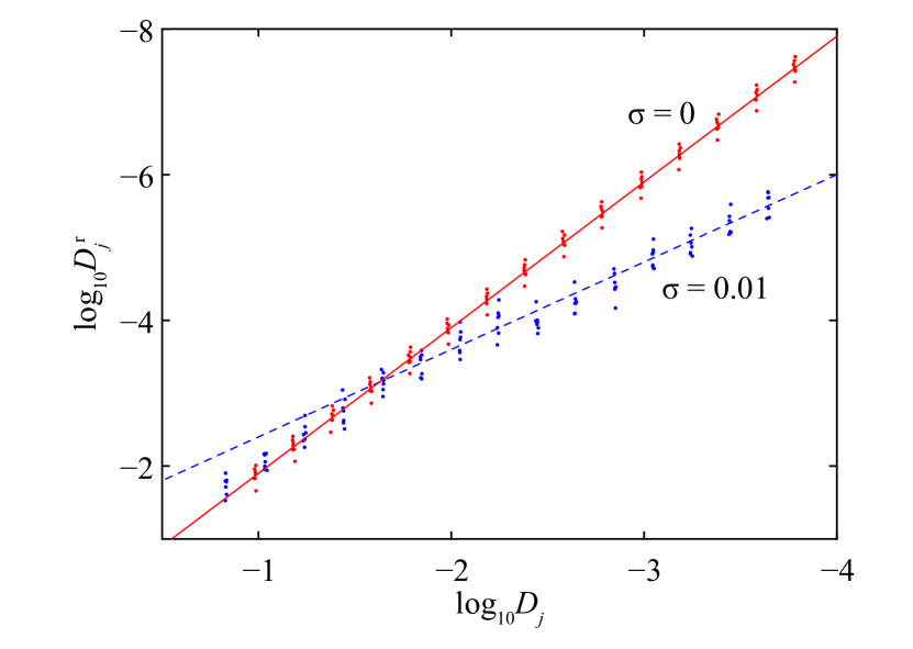
Figure 3: Distances of randomly generated noisy gates sets. Thirty gate sets are generated. Fifteen of them are reconstructed in the numerical simulation taking the sampling noise $\sigma=0.01$ (blue dots), and the other fifteen gate sets are reconstructed taking $\sigma=0$ (red dots). Error rates are in the range $\sim 10^{-3}-10^{-6}$. Straight lines are $\log_{10}D^{\rm r}_{j}=1.2\log_{10}D_{j}-1.2$ (blue) and $\log_{10}D^{\rm r}_{j}=2\log_{10}D_{j}+0.1$ (red), respectively. The slop grater than one means that the relative error decreases with the distance.

To use the result of the unital part in the reconstruction of the non-unital part, we need to find a proper similarity transformation. The unital part obtained using our protocol, which is denoted by $\hat{E}$, has an unknown similarity transformation from the actual unital part, i.e. $\hat{E}=BE{B}^{-1}$ (neglecting the sampling noise and higher-order effects in the perturbation). The matrix $B$ depends on how we choose the solution of Eq. (21). In the reconstruction of the non-unital part, the non-unital part of maps $(M_{i}M_{j})^{n}$ is measured using GST, and there is an unknown transformation from the actual non-unital part, i.e. $\hat{\vec{k}}^{\prime}=B^{\prime}\vec{k}+\vec{a}^{\prime}-B^{\prime}E{B^{\prime}}^{-1}\vec{a}^{\prime}$ is the result of GST. Here, the matrix $B^{\prime}$ depends on details of GST, including the state preparation and measurement error. Therefore, two matrices $B$ and $B^{\prime}$ are different in general. We need to find a proper similarity transformation relates the result of SOE (21) to the result of GST. Under the assumption that transformations from the actual map is close to identity, we can find the proper similarity transformation by solving equations. See Appendix B.1 for details.
In the reconstruction of the non-unital part, we first measure $21$ maps $(M_{i}M_{j})^{n}$ ($i<j$) using GST, where $n=\lfloor 1/p_{i,j}\rfloor$, where $p_{i,j}$ is the error rate of $M_{i}M_{j}$. The result is also used to determine the similarity transformation. In the numerical simulation, we take the result of the map $(M_{i}M_{j})^{n}$ as $T(M_{i}M_{j})^{n}T^{-1}+\zeta$, where $T$ is a randomly generated matrix representing unknown transformation from the actual map, and $\zeta$ is a matrix represents the sampling noise. $T$ is generated using the same approach for generating the noise in an actual map, and we take the error rate $p=0.1$. See Appendix A. Each element of $\zeta$ is generated according to the normal distribution with the zero mean and the standard deviation $\sigma=0.01$. Using the largest singular value of each double map, we have $21$ equations. The system of equations have $21$ unknown variables, corresponding to the non-unital part of the seven gates. However, three singular values of the system of equations (23) are small. To obtain a stable solution, we apply the truncation on singular values, i.e. replace the three small singular values with zero, and then determine the solution using the Moore-Penrose inverse.
To demonstrate that we can reconstruct high-fidelity gates with our protocol, we compare the reconstructed maps with actual maps. We use $M_{j}^{\rm r}$ to denote the reconstructed map. Because of the gauge problem, maps $M_{j}^{\rm r}$ and $M_{j}$ cannot be directly compared. Even our protocol is implemented ideally, the reconstruction is still up to an unknown similarity transformation, i.e. $TM_{j}^{\rm r}T^{-1}=M_{j}$. The matrix $T$ cannot be determined in GST because of the state preparation and measurement errors Greenbaum (2015). It is the same in our protocol. Therefore, the reconstruction is successful if there is a matrix $T$ such that $TM_{j}^{\rm r}T^{-1}-M_{j}$ is small for all $j$. We can find the matrix $T$ as shown in Appendix B.2. The result of $D^{\rm r}_{j}=\|TM_{j}^{\rm r}T^{-1}-M_{j}\|_{2}$ for noisy gate sets with different error rates are plotted in Fig. 3. We can find that the relative error of the reconstruction $D^{\rm r}_{j}/D_{j}$ decreases with $D_{j}$, where the distance $D_{j}=\|M_{j}-M_{j}^{\rm i}\|_{2}$ measures the error in the gate. Comparing results of the sampling noise $\sigma=0.01$ to the case without sampling noise, we can find that the sampling noise reduces the reconstruction accuracy when $D_{j}$ is smaller than $0.01$.
In our numerical simulation, we have use the prior knowledge of the gate error rate, such that we can choose the proper number of gate repetitions. In the practical implementation, we can choose the proper repetition number by measuring gate sequences for a set of repetition numbers, e.g. increasing the repetition number exponentially such as in the trace measurement. We note that the performance is not sensitive to the repetition number as shown in Figs. 1(a) and 2.

VI conclusion

In this paper we propose a protocol to reconstruct unknown quantum gates with high fidelity. This method reduces the impact of sampling noise by amplifying the error in deterministic gate sequences. Compared with analyzing data of gate sequences using the maximum likelihood estimation Blume-Kohout et al. (2017), our approach is based on solving linear equations rather than optimization algorithm. We can improve the accuracy of reconstruction by using the maximum likelihood estimation method and taking the result of our perturbative approach as the initial estimate of the error model. We demonstrate our protocol in numerical simulation and find that the relative error of reconstruction decreases with the gate error. Because our approach includes increasing the gate repetition number exponentially to approximately one over the error rate in the unital part reconstruction, the number of measurements needed in our protocol scales logarithmically with the error rate. However, because we need to amplify the error in sufficiently long gate sequences, the number of gates scales linearly. As long as the time cost of implementing gate sequences is practical, our protocol provides a way to choose proper gate sequences and efficiently reconstruct high fidelity quantum gates.

Our code used for generating numerical data in this paper can be found at code.

Appendix A Random error generation

Given the ideal map $\mathcal{M}^{\rm i}$ and the error rate $p$, we generate the map with error as follows. The Lindblad equation for a single qubit can be written as $\frac{d\rho}{dt}=\mathcal{L}(\rho)$, and

$$\mathcal{L}(\rho) = -i[H,\rho]$$ (24)

$$+\sum_{a,b=1}^{3}h_{a,b}\left[\sigma_{a}\rho\sigma_{b}-\frac{1}{2}(\sigma_{b}\sigma_{a}\rho+\rho\sigma_{b}\sigma_{a})\right]$$

Here, $H$ is the Hamiltonian, $h$ is a positive semidefinite matrix, and $\sigma_{a}$ are Pauli operators. To generate the error, we first randomly generate $H$ and $h$. The map with error is $\mathcal{M}=e^{\mathcal{L}t}\mathcal{M}^{\rm i}$, where $e^{\mathcal{L}t}$ represents the noise. By choosing the evolution time $t$, we can obtain the map with the desired error rate $p$. We use the same approach to generate the matrix $T$ of GST, by taking $T$ as the Pauli transfer matrix of $e^{\mathcal{L}t}$.

Appendix B Gauge freedom

According to the GST formalism, we can only determine the map in the tomography experiment up to a similarity transformation, i.e. two sets of maps $\{M_{i}\}$ and $\{TM_{i}T^{-1}\}$ are indistinguishable. All maps $\{M_{i}\}$ and $\{TM_{i}T^{-1}\}$ are in the form of Eq. (5), i.e. the first row is $(1,0,0,0)$, which sets four constraint conditions on $T$. Therefore, we can express $T$ as

$$T=\left[\begin{array}[]{cc}1&\vec{0}^{\rm\,T}\\ \vec{a}&B\end{array}\right].$$ (27)

We take the first element as one, because similarity transformations given by $T$ and $\alpha T$ are the same, where $\alpha$ is a non-zero scalar factor. The inverse matrix is

$$T^{-1}=\left[\begin{array}[]{cc}1&\vec{0}^{\rm\,T}\\ B^{-1}\vec{a}&B^{-1}\end{array}\right].$$ (30)

After the similarity transformation, we have

$$TMT^{-1}=\left[\begin{array}[]{cc}1&\vec{0}^{\rm\,T}\\ B\vec{k}+\vec{a}-BEB^{-1}\vec{a}&BEB^{-1}\end{array}\right].$$ (33)

We can find that the similarity transformation of $T$ causes a similarity transformation on the unital part, i.e. $E\rightarrow BEB^{-1}$. The matrix $B$ is $3\times 3$ and has $9$ elements. The similarity transformation is invariant when the matrix is scaled by a non-zero scalar factor. Therefore, the similarity transformation of the unital part has $8$ degrees of freedom, e.g. $8$ parameters cannot be determined in the reconstruction of the unital part.

To be specific, in our perturbative approach, we assume that $\delta M$ is small, which implies that $T$ is close to identity. Therefore, $\vec{a}$ and $\delta B\equiv B-\openone$ are small. The inverse matrix of $B$ is approximately $B^{-1}\simeq\openone-\delta B$. If we neglect high order terms, the error after the similarity transformation is

$$BEB^{\dagger}-E^{\rm i}\simeq\delta E+\delta BE^{\rm i}-E^{\rm i}\delta B.$$ (34)

We can find that if $\{\delta E_{j}\}$ is the solution of Eq. (21), $\{\delta E_{j}+\delta BE_{j}^{\rm i}-E_{j}^{\rm i}\delta B\}$ is also a solution. If we replace $\delta B$ with $\delta B+\alpha\openone$, where $\alpha$ is a scalar factor, the solution does not change. Therefore, there are $8$ non-trivial degrees of freedom.

The non-unital part after the similarity transformation is approximately $\vec{k}+\vec{a}-E^{\rm i}\vec{a}$. Here we have used that $B\approx\openone$ and $E\approx E^{\rm i}$. $E^{\rm i}$ is a unitary matrix, and one of its eigenvalues is one, which corresponds to the largest singular value in the non-unital part reconstruction. We only use the largest singular value in the non-unital part reconstruction, i.e. the non-unital part component that contributes to the reconstruction is $P(\vec{k}+\vec{a}-E^{\rm i}\vec{a})$, where $P$ is the projection operator onto the eigenvector (with the eigenvalue one) of $E^{\rm i}$. We can find that $P(\vec{k}+\vec{a}-E^{\rm i}\vec{a})=P\vec{k}$, i.e. if $\vec{k}$ is the solution to the equation of the non-unital part, $\vec{k}+\vec{a}-E^{\rm i}\vec{a}$ is also a solution. Because $\vec{a}$ has three elements, $3$ parameters cannot be determined in the reconstruction of the non-unital part.

We remark that in the discussion of the non-unital part, we have taken the approximations $B\approx\openone$ and $E\approx E^{\rm i}$. Because of the finite error in $B$ and $E$, we can find more than $3N-3$ linearly independent equations. However, the system of equations for the non-unital part has up to $3N-3$ singular values that are reasonably large.

B.1 Compute the transformation - Non-unital part

Let $\hat{E}$ and $\hat{E}^{\prime}$ be unital parts obtained by solving SOE (21) and GST, respectively. There are similarity transformations relate them to the actual unital part $E$, i.e. $\hat{E}=BE{B}^{-1}$ and $\hat{E}^{\prime}=B^{\prime}E{B^{\prime}}^{-1}$. Here, we have assumed that $\hat{E}$ and $\hat{E}^{\prime}$ are obtained without the sampling noise. We want to find $B^{\prime\prime}=B{B^{\prime}}^{-1}$ such that we can compute $\hat{E}^{\prime\prime}=B^{\prime\prime}\hat{E}^{\prime}{B^{\prime\prime}}^{-1}$. Ideally, we have $\hat{E}^{\prime\prime}=\hat{E}$.

Under the condition that the error in gates is small, maps obtained by solving SOE (21) and GST are both close to the ideal map. Therefore, matrices $B$, $B^{\prime}$ and $B^{\prime\prime}$ must be close to the identity matrix. We assume that $B^{\prime\prime}=\openone+\delta B$ and $\delta B$ is small.

Let $\hat{E}_{i}$ be the unital part of $M_{i}$ obtained by solving SOE (21). We compute $Y_{i,j}=(\hat{E}_{i}\hat{E}_{j})^{n}$. Let $X_{i,j}$ be the unital part of $(M_{i}M_{j})^{n}$ measured using GST. Then, we have equations

$$\delta BX_{i,j}-X_{i,j}\delta B=Y_{i,j}.$$ (35)

Here, we have neglected high-order terms of $\delta B$. We have $21$ double maps, therefore, $21\times 9=189$ equations. SOE (35) has $9$ unknown variables, but the rank is $8$. The variable that cannot be determined corresponds to scaling the similarity transformation matrix by a non-zero scalar factor, which is trivial. We solve SOE (35) using the Moore-Penrose inverse.

With the matrix $\delta B$, we compute $B^{\prime\prime}=\openone+\delta B$ and $\hat{\vec{k}}=B^{\prime\prime}\hat{\vec{k}}^{\prime}$. Then, $\hat{\vec{k}}$ is used as $\vec{k}$ ($\vec{k}_{i,j}^{(n)}$) in the reconstruction of the non-unital part.

B.2 Compute the transformation - Benchmarking

To compute the similarity transformation that relates $M_{j}^{\rm r}$ to $M_{j}$, we assume $TM_{j}^{\rm r}T^{-1}=M_{j}$, and $T$ is in the form given by Eq. (27). We assume $T$ is close to identity, i.e. $\vec{a}$ and $\delta B=B-\openone$ are small.

To compute $B$, we solve the equations

$$\delta BE_{j}^{\rm r}-E_{j}^{\rm r}\delta B=E_{j}.$$ (36)

Here, $E_{j}^{\rm r}$ is the unital part of the reconstructed gate $M_{j}^{\rm r}$, and $j=1,2,\ldots,7$. Here, we have neglected high-order terms of $\delta B$. We have $7$ maps, therefore, $7\times 9=63$ equations. As the same as in the case of SOE (35), there are $9$ unknown variables, but the rank is $8$. We solve SOE (36) using the Moore-Penrose inverse.

Given $\delta B$ and $B=\openone+\delta B$, we have equations

$$B\vec{k}_{j}^{\rm r}+\vec{a}-BE_{j}^{\rm r}B^{-1}\vec{a}=\vec{k}_{j},$$ (37)

where $\vec{k}_{j}^{\rm r}$ is the non-unital part of $M_{j}^{\rm r}$. We have $7$ maps, therefore, $7\times 3=21$ equations. There are $3$ unknown variables. We solve SOE (37) using the Moore-Penrose inverse.
In the computation of $T$, we assume that actual maps $M_{j}$ are known, which is only used for benchmarking the result in the numerical simulation and not needed in the implementation of our protocol.

References

- Nielsen and Chuang (2002) M. A. Nielsen and I. Chuang, Quantum computation and quantum information (2002).
- Barends et al. (2014) R. Barends, J. Kelly, A. Megrant, A. Veitia, D. Sank, E. Jeffrey, T. C. White, J. Mutus, A. G. Fowler, B. Campbell, et al., Superconducting quantum circuits at the surface code threshold for fault tolerance, Nature 508, 500 (2014).
- Harty et al. (2014) T. Harty, D. Allcock, C. J. Ballance, L. Guidoni, H. Janacek, N. Linke, D. Stacey, and D. Lucas, High-fidelity preparation, gates, memory, and readout of a trapped-ion quantum bit, Physical review letters 113, 220501 (2014).
- Beauregard (2002) S. Beauregard, Circuit for shor’s algorithm using 2n+ 3 qubits, arXiv preprint quant-ph/0205095 (2002).
- Steane (1996) A. M. Steane, Error correcting codes in quantum theory, Physical Review Letters 77, 793 (1996).
- Calderbank et al. (1997) A. R. Calderbank, E. M. Rains, P. W. Shor, and N. J. Sloane, Quantum error correction and orthogonal geometry, Physical Review Letters 78, 405 (1997).
- Fowler et al. (2012) A. G. Fowler, M. Mariantoni, J. M. Martinis, and A. N. Cleland, Surface codes: Towards practical large-scale quantum computation, Physical Review A 86, 032324 (2012).
- O’Gorman and Campbell (2017) J. O’Gorman and E. T. Campbell, Quantum computation with realistic magic-state factories, Physical Review A 95, 032338 (2017).
- Chiaverini et al. (2004) J. Chiaverini, D. Leibfried, T. Schaetz, M. D. Barrett, R. Blakestad, J. Britton, W. M. Itano, J. D. Jost, E. Knill, C. Langer, et al., Realization of quantum error correction, Nature 432, 602 (2004).
- Reed et al. (2012) M. D. Reed, L. DiCarlo, S. E. Nigg, L. Sun, L. Frunzio, S. M. Girvin, and R. J. Schoelkopf, Realization of three-qubit quantum error correction with superconducting circuits, Nature 482, 382 (2012).
- Li and Benjamin (2017) Y. Li and S. C. Benjamin, Efficient variational quantum simulator incorporating active error minimization, Physical Review X 7, 021050 (2017).
- Temme et al. (2017) K. Temme, S. Bravyi, and J. M. Gambetta, Error mitigation for short-depth quantum circuits, Physical review letters 119, 180509 (2017).
- Endo et al. (2018) S. Endo, S. C. Benjamin, and Y. Li, Practical quantum error mitigation for near-future applications, Physical Review X 8, 031027 (2018).
- Kandala et al. (2019) A. Kandala, K. Temme, A. D. Córcoles, A. Mezzacapo, J. M. Chow, and J. M. Gambetta, Error mitigation extends the computational reach of a noisy quantum processor, Nature 567, 491 (2019).
- Song et al. (2019) C. Song, J. Cui, H. Wang, J. Hao, H. Feng, and Y. Li, Quantum computation with universal error mitigation on a superconducting quantum processor, Science advances 5, eaaw5686 (2019).
- Zhang et al. (2020) S. Zhang, Y. Lu, K. Zhang, W. Chen, Y. Li, J.-N. Zhang, and K. Kim, Error-mitigated quantum gates exceeding physical fidelities in a trapped-ion system, Nature communications 11, 1 (2020).
- Emerson et al. (2005) J. Emerson, R. Alicki, and K. Życzkowski, Scalable noise estimation with random unitary operators, Journal of Optics B: Quantum and Semiclassical Optics 7, S347 (2005).
- Knill et al. (2008) E. Knill, D. Leibfried, R. Reichle, J. Britton, R. B. Blakestad, J. D. Jost, C. Langer, R. Ozeri, S. Seidelin, and D. J. Wineland, Randomized benchmarking of quantum gates, Physical Review A 77, 012307 (2008).
- Magesan et al. (2011) E. Magesan, J. M. Gambetta, and J. Emerson, Scalable and robust randomized benchmarking of quantum processes, Physical review letters 106, 180504 (2011).
- Magesan et al. (2012) E. Magesan, J. M. Gambetta, and J. Emerson, Characterizing quantum gates via randomized benchmarking, Physical Review A 85, 042311 (2012).
- Sheldon et al. (2016) S. Sheldon, L. S. Bishop, E. Magesan, S. Filipp, J. M. Chow, and J. M. Gambetta, Characterizing errors on qubit operations via iterative randomized benchmarking, Physical Review A 93, 012301 (2016).
- Fong and Merkel (2017) B. H. Fong and S. T. Merkel, Randomized benchmarking, correlated noise, and ising models, arXiv preprint arXiv:1703.09747 (2017).
- Proctor et al. (2017) T. Proctor, K. Rudinger, K. Young, M. Sarovar, and R. Blume-Kohout, What randomized benchmarking actually measures, Physical review letters 119, 130502 (2017).
- Wallman (2018) J. J. Wallman, Randomized benchmarking with gate-dependent noise, Quantum 2, 47 (2018).
- Onorati et al. (2019) E. Onorati, A. Werner, and J. Eisert, Randomized benchmarking for individual quantum gates, Physical review letters 123, 060501 (2019).
- Lu et al. (2015) D. Lu, H. Li, D.-A. Trottier, J. Li, A. Brodutch, A. P. Krismanich, A. Ghavami, G. I. Dmitrienko, G. Long, J. Baugh, et al., Experimental estimation of average fidelity of a clifford gate on a 7-qubit quantum processor, Physical review letters 114, 140505 (2015).
- McKay et al. (2019) D. C. McKay, S. Sheldon, J. A. Smolin, J. M. Chow, and J. M. Gambetta, Three-qubit randomized benchmarking, Physical review letters 122, 200502 (2019).
- Chuang and Nielsen (1997) I. L. Chuang and M. A. Nielsen, Prescription for experimental determination of the dynamics of a quantum black box, Journal of Modern Optics 44, 2455 (1997).
- Poyatos et al. (1997) J. Poyatos, J. I. Cirac, and P. Zoller, Complete characterization of a quantum process: the two-bit quantum gate, Physical Review Letters 78, 390 (1997).
- D’Ariano and Presti (2001) G. D’Ariano and P. L. Presti, Quantum tomography for measuring experimentally the matrix elements of an arbitrary quantum operation, Physical review letters 86, 4195 (2001).
- Altepeter et al. (2003) J. B. Altepeter, D. Branning, E. Jeffrey, T. Wei, P. G. Kwiat, R. T. Thew, J. L. O’Brien, M. A. Nielsen, and A. G. White, Ancilla-assisted quantum process tomography, Physical Review Letters 90, 193601 (2003).
- Mohseni and Lidar (2006) M. Mohseni and D. Lidar, Direct characterization of quantum dynamics, Physical review letters 97, 170501 (2006).
- Merkel et al. (2013) S. T. Merkel, J. M. Gambetta, J. A. Smolin, S. Poletto, A. D. Córcoles, B. R. Johnson, C. A. Ryan, and M. Steffen, Self-consistent quantum process tomography, Physical Review A 87, 062119 (2013).
- Blume-Kohout et al. (2013) R. Blume-Kohout, J. K. Gamble, E. Nielsen, J. Mizrahi, J. D. Sterk, and P. Maunz, Robust, self-consistent, closed-form tomography of quantum logic gates on a trapped ion qubit, arXiv preprint arXiv:1310.4492 (2013).
- Stark (2014) C. Stark, Self-consistent tomography of the state-measurement gram matrix, Physical Review A 89, 052109 (2014).
- Greenbaum (2015) D. Greenbaum, Introduction to quantum gate set tomography, arXiv preprint arXiv:1509.02921 (2015).
- Blume-Kohout et al. (2017) R. Blume-Kohout, J. K. Gamble, E. Nielsen, K. Rudinger, J. Mizrahi, K. Fortier, and P. Maunz, Demonstration of qubit operations below a rigorous fault tolerance threshold with gate set tomography, Nature communications 8, 1 (2017).
- Sugiyama et al. (2018) T. Sugiyama, S. Imori, and F. Tanaka, Reliable characterization of super-accurate quantum operations, arXiv preprint arXiv:1806.02696 (2018).
- Helsen et al. (2019) J. Helsen, F. Battistel, and B. M. Terhal, Spectral quantum tomography, npj Quantum Information 5, 1 (2019).
- Kimmel et al. (2014) S. Kimmel, M. P. da Silva, C. A. Ryan, B. R. Johnson, and T. Ohki, Robust extraction of tomographic information via randomized benchmarking, Physical Review X 4, 011050 (2014).
- Govia et al. (2020) L. Govia, G. Ribeill, D. Ristè, M. Ware, and H. Krovi, Bootstrapping quantum process tomography via a perturbative ansatz, Nature communications 11, 1 (2020).
- Choi (1975) M.-D. Choi, Completely positive linear maps on complex matrices, Linear algebra and its applications 10, 285 (1975).
- Jordan et al. (2004) T. F. Jordan, A. Shaji, and E. Sudarshan, Dynamics of initially entangled open quantum systems, Physical Review A 70, 052110 (2004).
- Rudnicki et al. (2018) Ł. Rudnicki, Z. Puchała, and K. Zyczkowski, Gauge invariant information concerning quantum channels, Quantum 2, 60 (2018).
- Huo and Li (2018) M. Huo and Y. Li, Self-consistent tomography of temporally correlated errors, arXiv , arXiv (2018).
- Wolberg (2006) J. Wolberg, Data analysis using the method of least squares: extracting the most information from experiments (Springer Science & Business Media, 2006).
- Sarkar and Pereira (1995) T. K. Sarkar and O. Pereira, Using the matrix pencil method to estimate the parameters of a sum of complex exponentials, IEEE Antennas and Propagation Magazine 37, 48 (1995).
- Ben-Israel and Greville (2003) A. Ben-Israel and T. N. Greville, Generalized inverses: theory and applications, Vol. 15 (Springer Science & Business Media, 2003).